Article

Theoretical Properties of Closed Frequent Itemsets in Frequent Pattern Mining

1
School of Mathematics and Statistics, Beijing Technology and Business University, Beijing 100048, China
2
School of Mathematics, Harbin Institute of Technology, Harbin 150001, China
*
Author to whom correspondence should be addressed.
Mathematics 2025, 13(11), 1709; https://doi.org/10.3390/math13111709
Submission received: 10 April 2025 / Revised: 15 May 2025 / Accepted: 20 May 2025 / Published: 23 May 2025
(This article belongs to the Special Issue Advances in Statistical AI and Causal Inference)

Abstract

:
Closed frequent itemsets (CFIs) play a crucial role in frequent pattern mining by providing a compact and complete representation of all frequent itemsets (FIs). This study systematically explores the theoretical properties of CFIs by revisiting closure operators and their fundamental definitions. A series of formal properties and rigorous proofs are presented to improve the theoretical understanding of CFIs. Furthermore, we propose confidence interval-based closed frequent itemsets (CICFIs) by integrating frequent pattern mining with probability theory. To evaluate the stability, three classical confidence interval (CI) estimation methods of relative support (rsup) based on the Wald CI, the Wilson CI, and the Clopper–Pearson CI are introduced. Extensive experiments on both an illustrative example and two real datasets are conducted to validate the theoretical properties. The results demonstrate that CICFIs effectively enhance the robustness and interpretability of frequent pattern mining under uncertainty. These contributions not only reinforce the solid theoretical foundation of CFIs but also provide practical insights for the development of more efficient algorithms in frequent pattern mining.

1. Introduction

Frequent itemset mining (FIM) is a fundamental task in frequent pattern mining, aiming to identify itemsets that frequently co-occur in transaction datasets. A typical application example is the market basket analysis, wherein commodities purchased together are identified. However, traditional FIM methods usually suffer from the problem of exponential growth in the number of itemsets, especially when a low support threshold is applied, leading to substantial redundancy among candidate itemsets. To address this problem, a CFI is introduced as a condensed representation of frequent itemsets. The mining process of CFIs aims to discover a compact and lossless representation of all frequent itemsets, thereby significantly reducing the computational complexity and storage requirements. The compactness makes CFIs a promising research direction and provides prospective insights for developing more efficient algorithms in data mining.
Several research works have been conducted on frequent pattern mining, as it has been widely applied in various domains, such as gene expression pattern discovery [1], disease diagnosis [2], and optimizing commodity association rules and recommendation systems [3,4]. With in-depth and continuous research, numerous efficient algorithms have been proposed. Specifically, the Closet and Closet+ algorithms [5] were proposed based on FP-Growth. As a further optimization method, QCloSET+ [6] extends Closet+ by reducing the number of database scans to a single pass for frequent itemset mining. In addition, a method for mining frequent weighted closed itemsets (FWCIs) [7] from weighted item transaction databases was proposed. For the fast mining of closed frequent itemsets, NECLATCLOSED [8] was presented as a vertical algorithm. Two efficient algorithms named DFI-List and DFI-Growth [9] were introduced by adopting depth-first search and divide-and-conquer methodology. Additionally, several other algorithms were presented, including but not limited to CICLAD [10], GrAFCI+ [11], and MMC [12], which play significant roles in closed frequent itemset mining.
Although extensive research has been conducted on CFIs, most existing studies have primarily focused on algorithm improvement, with relatively limited attention given to the deep exploration of their underlying properties. The lack of systematic investigations into the theoretical properties of CFIs highlights the need for further research. This paper aims to establish a series of theoretical properties and theorems, supported by rigorous proofs and experimental validation. The main contributions are summarized as follows:
(1)
The proposed properties and theorems strengthen the theoretical foundation of CFIs and facilitate an efficient determination of whether an itemset is both frequent and closed. As CFIs serve as a compressed and lossless representation, all FIs, including their support values, can be derived from CFIs.
(2)
Each equivalence class contains a unique maximal itemset, denoted as the CFIs. All FIs within the same equivalence class share identical transaction identifiers and support values, ensuring redundancy reduction in pattern mining.
(3)
A novel concept of CICFIs is introduced, accompanied by three confidence interval estimation methods under the assumption that support follows a binomial distribution. These methods provide a more robust assessment of the stability of CFIs, contributing to the reliability of frequent pattern mining results.
(4)
Comprehensive experiments are conducted to strengthen the practical validation of the properties. The experimental results show that the CICFIs and three distinct methods play significant roles in improving reliability in frequent pattern mining.
The remainder of this paper is organized as follows: Section 2 introduces the relevant preliminary knowledge. Section 3 presents novel properties and theorems, particularly the concept of CICFIs and the three confidence intervals, together with their rigorous proofs and a detailed analysis of the experiments. Finally, conclusions and future research directions are given in Section 4.

2. Preliminaries

In this section, we introduce the basic knowledge and definitions of frequent pattern mining. Let I = { i 1 , i 2 , , i n } be a finite set of n distinct items. Subset X = { i 1 , i 2 , , i k } such that X I is called k i t e m s e t s , in which k is the length of the itemset. Let T = { t 1 , t 2 , , t m } be a set of all transaction identifiers with the total number m. Each transaction is a tuple in the form of t , X , in which t T and X represent a unique identifier and an itemset, respectively. To simplify the notation, the transaction identifier t is used to denote a transaction represented as t , X . Let D T × I be a transaction dataset, indicating the binary relationship between the set of transaction identifiers T and the set of items I . A transaction t T is said to contain the item x I if and only if ( t , x ) D . Moreover, a transaction t contains the itemset X = { i 1 , i 2 , , i k } if and only if t , x i D ( i = 1 , 2 , , k ) .
A sample dataset is given in Table 1. Here, T = { t 1 , t 2 , t 3 , t 4 , t 5 , t 6 , t 7 } represents the seven transaction identifiers (Tids). I = { A , B , C , D , E } denotes five distinct items or products purchased by customers.
Definition 1
 (support [13]). The support of an itemset X is the number of all transaction identifiers containing itemset X in dataset D, defined as
s u p ( X ) = | { t | < t , i ( t ) > D a n d X i ( t ) } | = | t ( X ) | .
The relative support (rsup) is the relative frequency, as well as the proportion of transactions containing X in database D, denoted as
r s u p ( X ) = s u p ( X ) | D | .
E.g., in the sample dataset, s u p ( A ) = | { t 1 , t 3 , t 4 , t 5 } | = 4 , s u p ( A B C ) = | { t 3 , t 5 } | = 2 . r s u p ( A ) = 4 / 7 , s u p ( A B C ) = 2 / 7 .
Definition 2
 (frequent itemsets [13], FIs). If s u p ( X ) m i n s u p , where m i n s u p is the minimum support threshold, itemset X in dataset D is frequent.
E.g., let m i n s u p = 4 . The set of FIs in the sample dataset are shown in Table 2.
Definition 3.
Let t : 2 I 2 T be a function that maps the set of items to the set of transaction identifiers. Define t ( X ) = { t T | t c o n t a i n s X } , where X I , and t ( X ) is the collection set of all transaction identifiers that contain itemset X.
E.g., in the sample dataset, let X = A B , t ( A B ) = { t 1 , t 3 , t 4 , t 5 } .
Definition 4.
Let i : 2 T 2 I be a function that maps the set of transaction identifiers to the set of items. Define i ( T ) = { x I | t T , t c o n t a i n s x } , where T T , and i ( T ) is a collection of common itemsets containing all transaction identifiers of itemset X.
E.g., in the sample dataset, let T = { t 1 , t 2 , t 3 } , i ( T ) = i ( { t 1 , t 2 , t 3 } ) = B E .
Definition 5
 (closure operator [14]). Let c : 2 I 2 I be the closure operator, defined as follows: c ( X ) = i o t ( X ) = i ( t ( X ) ) . Then, c ( X ) is the closure of itemset X. If itemset X satisfies the equation c ( X ) = X , itemset X is closed.
E.g., let X = A B , t ( A B ) = { t 1 , t 3 , t 4 , t 5 } , c ( A B ) = i o t ( A B ) = i ( { t 1 , t 3 , t 4 , t 5 } ) = A B E . Let X = A B E , c ( A B E ) = i o t ( A B E ) = i ( { t 1 , t 3 , t 4 , t 5 } ) = A B E ; itemset A B E is closed.
Definition 6
 (closed frequent itemsets [15], CFIs). If itemset X is both frequent and closed, we call it a closed frequent itemset.
E.g., let X = A B E , s u p ( A B E ) = 4 , c ( A B E ) = i o t ( { t 1 , t 3 , t 4 , t 5 } ) = A B E . Obviously, A B E is a closed frequent itemset.
Definition 7
 (equivalent class [16]). Given two itemsets X and Y, if they are contained in the same set of transactions, they are considered to be equivalent. Formally, for any itemset X, its equivalent class is expressed as
[ X ] = { Y I | t ( Y ) = t ( X ) } ,
where t ( X ) and t ( Y ) denote the set of transaction identifiers in which itemsets X and Y appear, respectively.
E.g., let X = A B , Y = A E ; then, t ( A B ) = t ( A E ) = { t 1 , t 3 , t 4 , t 5 } , and itemsets A B and A E are equivalent because they occur in the same transactions. In general, the equivalent class of A B is [ A B ] = { A , A B , A E , A B E } , and the closure of all itemsets in the same equivalence class is identical.
In the sample dataset, the equivalent class, closure, and its corresponding set of Tids on FIs are shown in Table 3.

3. Main Results and Their Demonstrations

In this section, a series of properties and theorems related to the closure operator and CFIs are proposed by reviewing their fundamental definitions. Theoretical derivations and rigorous proofs are provided to establish a solid foundation for closed frequent itemset mining. Furthermore, the concept of CICFIs is introduced, along with three confidence interval estimation methods, the Wald CI, the Wilson CI, and the Clopper–Pearson CI, to enhance the reliability of frequent pattern mining. Finally, experiments and result analysis are conducted to validate the stability and practical applicability of the proposed methods.

3.1. Properties and Theorems

According to Definitions 3 and 4, a connection to monotonicity can be established, summarizing the following theorem formulation. Theorem 1 provides valuable insights into closure operators and closed frequent itemset mining.
Theorem 1.
Functions t and i are monotone functions. Specifically,
(1) If X m X n ( m n ) , there is t ( X n ) t ( X m ) . Function t monotonically decreases.
(2) If T m T n ( m n ) , there is i ( X n ) i ( X m ) . Function i monotonically decreases.
Proof. 
(1) If X m X n ( m n ) , we know that X m is a subset of X n . So, we have s u p ( X n ) s u p ( X m ) , which is equivalent to | t ( X n ) | | t ( X m ) | . Then, t ( X n ) t ( X m ) . Thus, function t monotonically decreases.
(2) If T m T n ( m n ) , there is | T n | | T m | , which means that | i ( T n ) | | i ( T m ) | . Then, we obtain i ( X n ) i ( X m ) . Thus, function i monotonically decreases. □
Regarding the properties of closure operators, the following three properties are defined in the literature [17], but no relevant proofs are introduced. Here, detailed proofs are presented for a deep understanding of the closure operator according to the definition of closure operators [14,18].
Property 1.
The closure operator c satisfies the following properties:
(1) Extensive: X C ( X ) .
(2) Monotonic: If X i X j , then c ( X i c ( X j ) ) .
(3) Idempotent: c ( c ( X ) ) = c ( X ) .
Proof. 
(1) According to the definition of the closure operator, c ( X ) represents the common itemsets of all transaction identifiers containing itemset X. Since the set of all transaction identifiers containing itemset X already includes itself, itemset X must be contained within the set. Thus, we obtain X c ( X ) . Conversely, if x X , it is obvious that item x will also appear in the transaction identifier set containing itemset X. Consequently, we have X c ( X ) . (1) Thus, the extensiveness property of the closure operator holds.
(2) As Theorem 1 describes, if X i X j , there is t ( X i ) t ( X j ) . Then, it follows that i o t ( X i ) i o t ( X j ) , expressed as c ( X i ) c ( X j ) . Thus, the monotonicity property of the closure operator holds.
(3) Based on the extensiveness and monotonicity properties of the closure operator, we have X c ( X ) . Then, c ( X ) c ( c ( X ) ) , as c ( X ) is the maximum set of common itemsets of all the transaction identifiers containing itemset X. So, it follows that c ( X ) c ( c ( X ) ) . Thus, the idempotent property of the closure operator holds. □
As defined by the closure operator, c ( X ) is the intersection of all transactions that contain itemset X. Thus, the closure of a frequent itemset must exist and be unique. In addition, the closure of an itemset has the same support value as the itemset itself, i.e., sup(c(X)) = sup(X). Furthermore, a frequent itemset is considered closed [9] if and only if it has no proper superset Y X such that s u p ( Y ) = s u p ( X ) . In other words, if X is closed, then, for all Y X , it holds that s u p ( X ) > s u p ( Y ) . These properties provide a solid theoretical basis for understanding the relationship between closures and their support values. Based on these foundations, the key properties of CFIs are summarized.
Property 2.
The properties of CFIs are as follows:
(1) Itemsets with the same transaction identifiers only have at most one closed frequent itemset.
(2) A set of CFIs can uniquely determine the support value of all FIs, i.e., x F , Y C , s . t . X Y a n d s u p ( X ) = s u p ( Y ) .
(3) For any itemset, the number of its CFIs will not exceed the number of FIs, i.e., | C ( X ) | | F ( X ) | .
Proof. 
(1) As itemsets that share the same transaction identifiers belong to the same equivalent class, their closure must exist and be unique according to Theorem 3. Thus, itemsets within the same equivalence class can have at most one closed itemset.
(2) Let Y C be the closure of frequent itemset X. Then, Y is the maximal itemset among all itemsets with the same transaction identifiers as itemset X, s.t. X Y and s u p ( X ) = s u p ( Y ) . Thus, for each frequent itemset X, there exists a closed frequent itemset Y that has the same support value. In other words, every frequent itemset can be derived from their corresponding CFIs.
(3) According to the definition of CFIs, the process of obtaining CFIs aims to discover the maximum itemsets in the set of FIs that have the same support value. Hence, each set of CFIs is a subset of the corresponding FIs, denoted as C ( X ) F ( X ) . However, not all FIs are closed. Based on the completeness property of CFIs, every frequent itemset can be derived from an equivalence class of CFIs. Therefore, the number of CFIs must not exceed the number of all FIs, i.e., | C ( X ) | | F ( X ) | . □
Moreover, the equivalence class of CFIs exhibits certain properties that reveal deeper structural relationships among frequent patterns.
Property 3.
The equivalence class of FIs satisfies the following two properties:
(1) If itemsets X and Y are frequent and have the same closure, i.e., C ( X ) = C ( Y ) , then they are equivalent and have the same support values s u p ( X ) = s u p ( Y ) .
(2) For each equivalent class [ X ] , there exists a unique maximum itemset C ( X ) that is also a closed frequent itemset, satisfying
C ( X ) = Y [ X ] Y a n d T ( C ( X ) ) = T ( X ) .
Proof. 
(1) Let C ( X ) and C ( Y ) denote the maximum common itemsets of all transaction identifiers that contain itemsets X and Y, respectively. Since C ( X ) = C ( Y ) , it implies that itemsets X and Y have the same transaction identifiers, i.e., T ( X ) = T ( Y ) . Then, s u p ( X ) = | T ( X ) | = | T ( Y ) | = s u p ( Y ) . Thus, itemsets X and Y are equivalent and have the same support value.
(2) First, let C ( X ) = Y [ X ] Y be the union set of all itemsets with the same support value as itemset X. Clearly, Y [ X ] , and we have Y C ( X ) . Thus, C ( X ) is the largest itemset containing all itemsets in the equivalence class [ X ] .
Second, for the forward direction, T ( C ( X ) ) = T ( X ) . On the one hand, t T ( C ( X ) ) , transaction t contains itemset C ( X ) . Y [ X ] , itemset Y, and the equivalent class of itemset [ X ] share the same transaction identifiers, i.e., T ( X ) = T ( Y ) . This means that all the items in Y are contained in transaction t. Then, t T ( Y ) = T ( X ) . Thus, T ( C ( X ) ) T ( X ) . Conversely, t T ( X ) , transaction t contains itemset X. Meanwhile, if Y [ X ] , there is T ( X ) = T ( Y ) . Then, both itemsets Y and C ( X ) = Y [ X ] Y are contained in transaction t. Thus, T ( X ) T ( C ( X ) ) .
Third, since C ( X ) is defined as the union of all itemsets in the equivalence class [ X ] , we have C ( X ) = Y [ X ] Y , which means that C ( X ) is the maximum itemset among all itemsets in [ X ] . Y [ X ] , there is Y C ( X ) . Suppose that there exists another maximum itemset C ( X ) [ X ] such that C ( X ) C ( X ) . Y [ X ] ; there is Y C ( X ) . So, C ( X ) = Y [ X ] Y C ( X ) . Similarly, as C ( X ) is the maximum itemset, there also exists C ( X ) = Y [ X ] Y C ( X ) . So, we have C ( X ) = C ( X ) , which contradicts the assumption that C ( X ) C ( X ) . Thus, C ( X ) is unique. □
Building upon these equivalence class properties, we can derive several important corollaries that further characterize the structure, representation, and partitioning behavior of frequent itemsets within the closed itemset framework.
Corollary 1.
Each equivalence class of frequent itemsets can typically be represented by a unique representative element, which corresponds to the closed frequent itemset that encompasses all elements within the equivalence class.
Corollary 2.
If two equivalence classes are distinct, their intersection is empty; i.e., if [ X ] [ Y ] , then [ X ] [ Y ] = .
Corollary 3.
Under the defined equivalence class, the set of FIs can be decomposed into multiple disjoint equivalence classes, whose union collectively represents a complete set of frequent itemsets.
Let N be the the total number of transaction identifiers in dataset D, and let K be the occurrence number of itemset X in D. Suppose that each transaction can be regarded as a Bernoulli experiment in which the itemset that appears in the transaction is considered “True” and otherwise “False”; the support value of itemset X is the occurrence number in the N times of Bernoulli experiments such that K = s u p ( X ) and its corresponding probability are estimated by rsup. Then, the support values follow the binomial distribution:
s u p ( X ) = K B i n ( N , p ˜ ) ,
where p ˜ = r s u p ( X ) = s u p ( X ) | D | = K N .
In real-world scenarios, big data and uncertain dynamic data are common, making it difficult and impractical to obtain the exact values of support and relative support directly. One feasible solution is to estimate the values by using sample data. However, due to the potential error in the point estimation, confidence intervals are introduced to provide a more robust evaluation. In statistics, a confidence interval is a range of values used to estimate an unknown population parameter, typically accompanied by a confidence level that represents the probability that the true parameter lies within this range [19]. Generally, a narrower confidence interval width indicates a more precise estimate of the population parameter, whereas a wider confidence interval width implies a more conservative estimation. Based on these foundations, the concept of a confidence interval-based closed frequent itemset (CICFI) and its associated properties are discussed by integrating confidence intervals into closed frequent itemset mining, aiming to evaluate the stability of the discovered CFIs under data uncertainty.
Definition 8 (confidence interval-based closed frequent itemsets, CICFIs).
Let 1 α be the confidence level. The rsup value of a frequent itemset X is within the interval [ P L , P U ] , satisfying P ( P L r s u p ( X ) P U ) 1 α . If X is closed and P L θ , where θ is the minimum threshold, itemset X is a CICFI.
Theorem 2.
Let 1 α be the confidence level. X I , if itemset X is a CICFI, and the probability estimate value of the occurrence number of itemset X is p ˜ = r s u p ( X ) = K N , the confidence intervals of rsup can be expressed as follows:
(1) (Wald confidence interval, Wald CI). When the sample size N is very large and p ˜ is not an extreme value (such as 0 or 1), r s u p ( X ) can be approximated by a normal distribution, and its corresponding Wald CI is
p ˜ z α / 2 · p ˜ ( 1 p ˜ ) N , p ˜ + z α / 2 · p ˜ ( 1 p ˜ ) N ,
where z α / 2 is the 1 α 2 quantile point of the standard normal distribution.
(2) (Wilson confidence interval, Wilson CI). This is an improvement of the Wald confidence interval by correcting the bias and instability. The Wilson CI is
p ˜ + z α / 2 2 2 N z α / 2 · p ˜ ( 1 p ˜ ) N + z α / 2 2 4 N 2 1 + z α / 2 2 N , p ˜ + z α / 2 2 2 N + z α / 2 · p ˜ ( 1 p ˜ ) N + z α / 2 2 4 N 2 1 + z α / 2 2 N ,
where z α / 2 is the 1 α 2 quantile point of the standard normal distribution.
(3) (Clopper–Pearson confidence interval, Clopper–Pearson CI). Based on the cumulative distribution function (CDF) of a binomial distribution, this presents an exact confidence interval suitable for an arbitrary sample size. The Clopper–Pearson CI can be expressed by the quantiles of the B e t a distribution as follows:
B e t a 1 ( α 2 ; K , N K + 1 ) , B e t a 1 ( 1 α 2 ; K + 1 , N K ) ,
where α 2 and 1 α 2 are the quantile, and B e t a 1 is the inverse cumulative distribution function of B e t a .
Proof. 
(1) Suppose that p and p ( 1 p ) N are the expectation and variance of p ˜ , respectively. According to the Central Limit Theorem (CLT), p ˜ approximately follows the normal distribution, p ˜ N ( N , p ( 1 p ) N ) . From the properties of the normal distribution, we can obtain
P p ˜ z α / 2 · p ˜ ( 1 p ˜ ) N p p ˜ + z α / 2 · p ˜ ( 1 p ˜ ) N 1 α .
Thus, the Wald CI is
p ˜ z α / 2 · p ˜ ( 1 p ˜ ) N , p ˜ + z α / 2 · p ˜ ( 1 p ˜ ) N .
(2) Let the standard normal score be
p ˜ p p ( 1 p ) N z α / 2 .
By squaring both sides, we have
( p ˜ p ) 2 p ( 1 p ) N z α / 2 2 .
Then,
( N + z α / 2 2 ) · p 2 ( 2 N p ˜ + z α / 2 2 ) · p + N · p ˜ 2 = 0 .
Let A = N + z α / 2 2 ) , B = ( 2 N p ˜ + z α / 2 2 ) , and C = N · p ˜ 2 ; the above formula can be converted to a quadratic equation with one variable as A · p 2 + B · p + C = 0 . The solution is
p = 2 N p ˜ 2 + z α / 2 2 ± z α / 2 · α / 2 + 4 N p ˜ ( 1 p ˜ ) 2 ( N + z α / 2 2 ) .
Thus, the Wilson CI is
p ˜ + z α / 2 2 2 N z α / 2 · p ˜ ( 1 p ˜ ) N + z α / 2 2 4 N 2 1 + z α / 2 2 N , p ˜ + z α / 2 2 2 N + z α / 2 · p ˜ ( 1 p ˜ ) N + z α / 2 2 4 N 2 1 + z α / 2 2 N .
(3) Since s u p ( X ) = K B ( N , p ) , its probability mass function is
P ( K = k ) = N k p k ( 1 p ) N k , k = 0 , 1 , 2 , , N .
Based on the Clopper–Pearson method, the confidence intervals are constructed by controlling the tail probabilities on both sides such that the probability p is at least 1 α as follows:
P ( K k | P L ) = i = k N N i p i ( 1 p ) N i α 2 ,
P ( K k | P L ) = i = 0 k N i p i ( 1 p ) N i α 2 .
Because of the dual relationship of the binomial and Beta distribution, there is
P ( K k | P ) = I p ( x , n x + 1 ) , P ( K k | P ) = 1 I p ( x + 1 , n x ) ,
where I p is the cumulative probability function of the B e t a distribution.
So,
I P L ( K , N K + 1 ) = α 2 , 1 I P U ( K + 1 , N X ) = α 2 .
Then,
P L = B e t a 1 ( α 2 ; K , N K + 1 ) , P U = B e t a 1 ( 1 α 2 ; K + 1 , N X ) .
Thus, the Clopper–Pearson CI is
[ B e t a 1 ( α 2 ; K , N K + 1 ) , B e t a 1 ( 1 α 2 ; K + 1 , N K ) ] .

3.2. Experiments and Result Analysis

In order to gain a deeper understanding of the theoretical significance, extensive experiments were conducted with the aforementioned example dataset, as well as two real datasets, retail and mushroom. The properties and theorems were first verified on the example dataset. Furthermore, the two real datasets were introduced in the following verified experiments of the proposed CICFIs to strengthen the practical applications. All datasets were downloaded from the SPMF repository [20], and their characteristics are summarized in Table 4.
(1)
Experiments on the example dataset
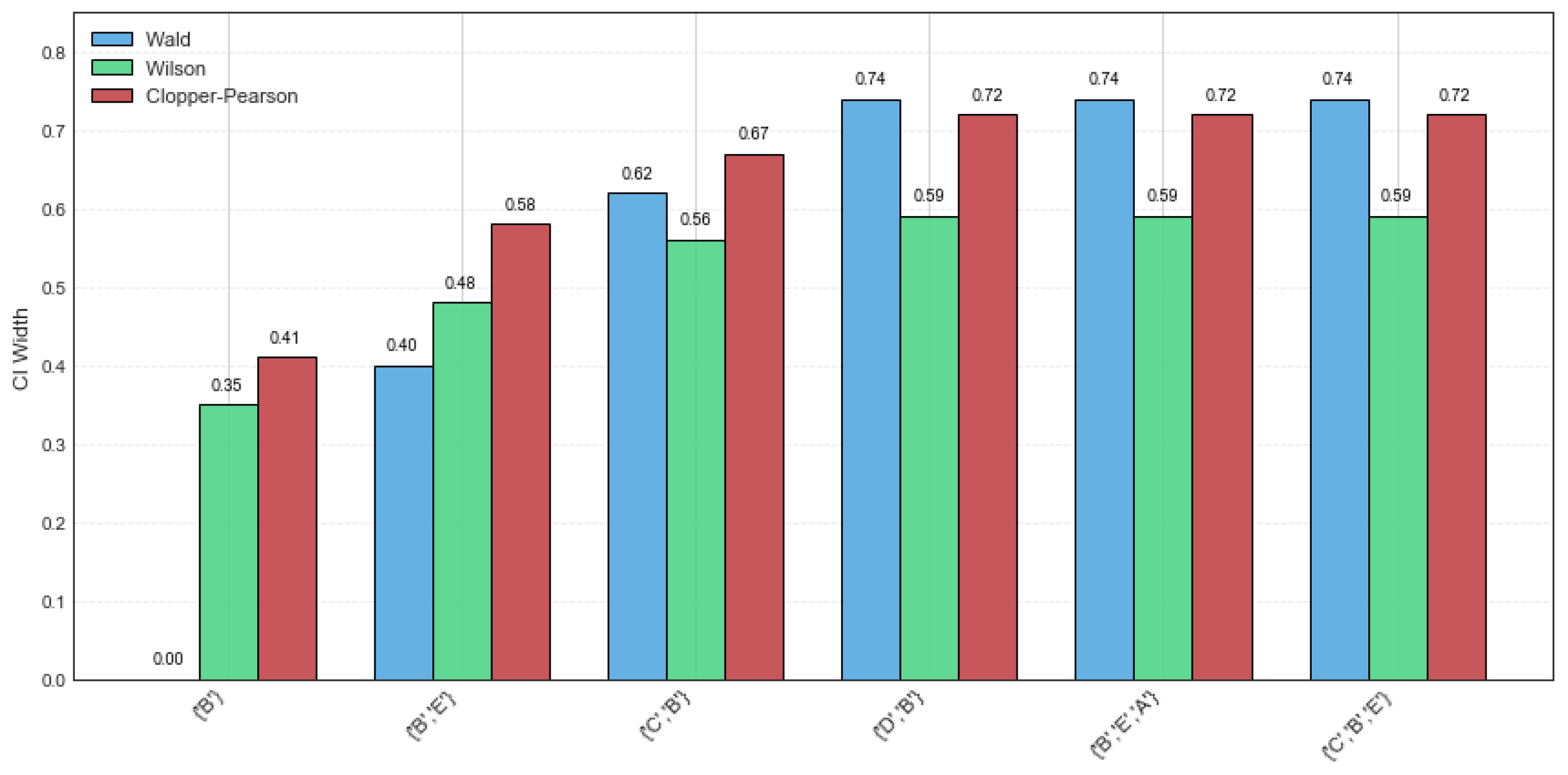
The confidence intervals of the Wald, Wilson, and Clopper–Pearson methods for CFIs on the example dataset are presented in Table 5. It can be derived that the width of the confidence intervals is too large, so the estimate values are not exact. Specifically, a width comparison of the Wald, Wilson, and Clopper–Pearson CI methods on various CFIs is shown in Figure 1. It can be observed that the Wald method performs more favorably for itemsets {‘B’} and {‘B’, ‘E’}, with high support values and a narrow CI width. This indicates that these two itemsets have a high probability and occurrence frequency, demonstrating good stability. However, potential risks and instability will occur when rsup decreases. In comparison, the Wilson method demonstrates greater stability and practical applicability, whereas the Clopper–Pearson method produces the widest confidence intervals.
(2)
Experiments on two real datasets
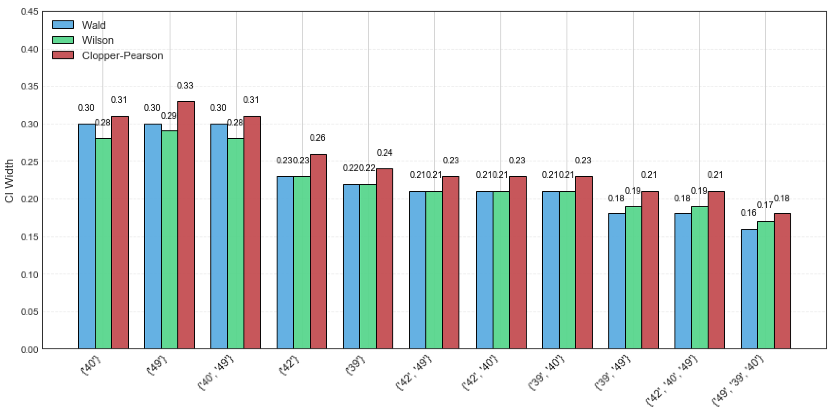
The retail dataset is a sparse dataset consisting of 88,162 transactions and 16,407 distinct itemsets, with an average transaction length of 10.3 and a maximum length of 76. As the dataset contains various itemsets, the random sampling size was set to 40, and the minimum support threshold was set to 6% for a more intuitive visualization. The results of the three distinct confidence intervals for CFIs on the retail dataset are presented in Table 6. Figure 2 shows a width comparison of the Wald, Wilson, and Clopper–Pearson CI methods across various CFIs for the same dataset. It can be observed that the Wald and Wilson methods exhibit better stability, as evidenced by their narrower confidence interval widths. However, the Clopper–Pearson CI method shows the highest coverage probability, reflecting its robustness to data variations. In addition, compared to the example dataset, the CI widths of the CFIs on the retail dataset are generally smaller. This shows that the larger the sample sizes, the better the confidence interval estimation precision.
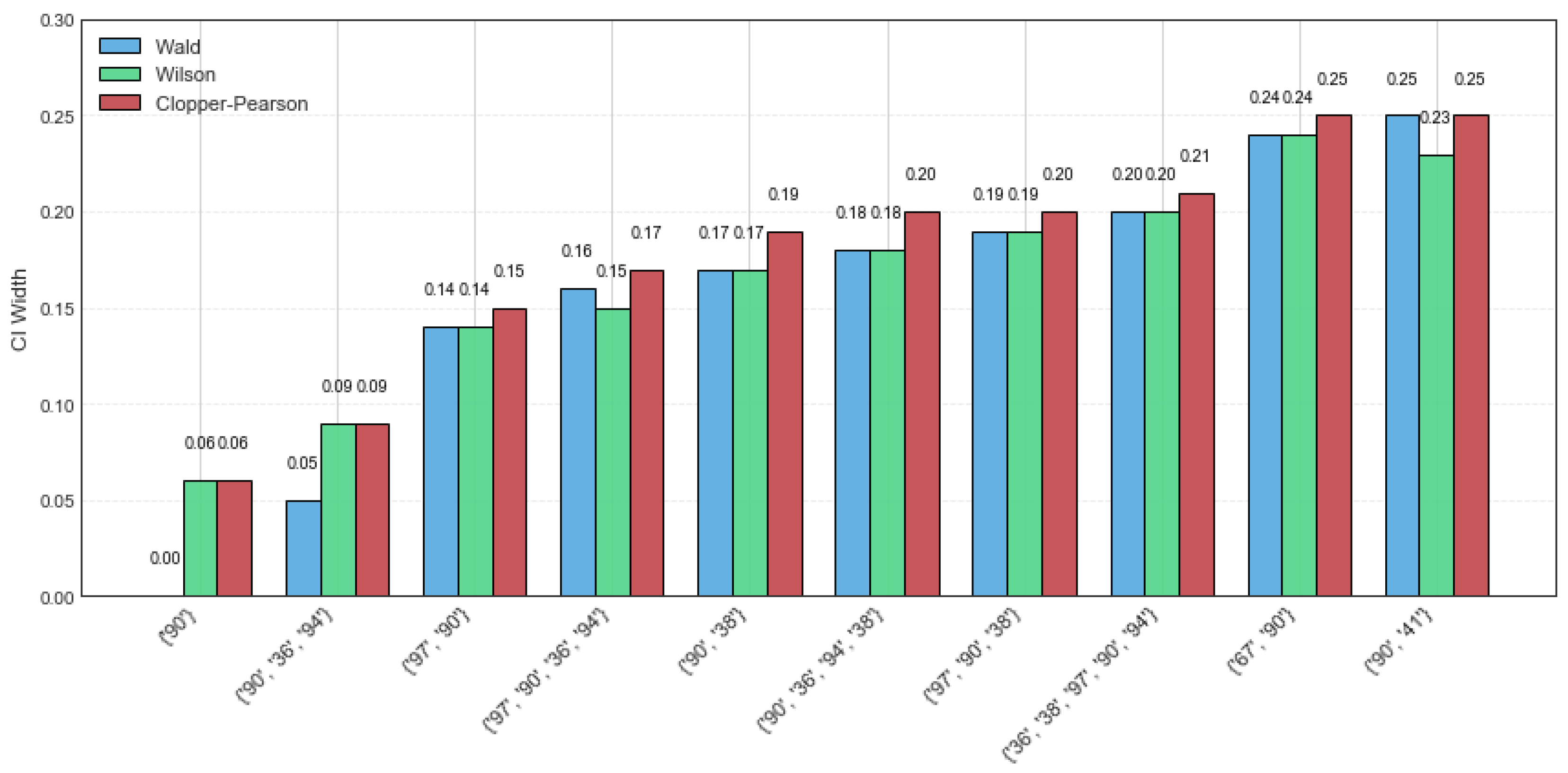
The mushroom dataset consists of 8124 transactions with 119 distinct items, and both the average transaction length and maximum transaction length are 23. In this experiment, the random sample size is set to 60, with minsup = 60%. The CI estimation results of the Wald, Wilson, and Clopper–Pearson CI methods are summarized in Table 7. Notably, all three methods perform well, particularly for the itemsets {‘90’} and {‘90’, ‘36’, ‘94’}, where the maximum CI width across all methods does not exceed 0.09. As the rsup value increases, the width of the confidence intervals becomes narrower. In other words, the estimated value of rsup lies within the confidence interval with a high probability. A narrower confidence interval suggests that the estimation is not only more precise but also more stable. Figure 3 presents a detailed comparison of the CI width on the mushroom dataset for the top ten CFIs. The Wald CI demonstrates satisfactory performance under high rsup, but it tends to be unstable when the rsup value is low. On the contrary, the Clopper–Pearson CI exhibits greater robustness, as its CI width is large, showing a higher tolerance for data variability. Among the three methods, the Wilson method achieves superior performance by providing a balanced trade-off between interval precision and stability.
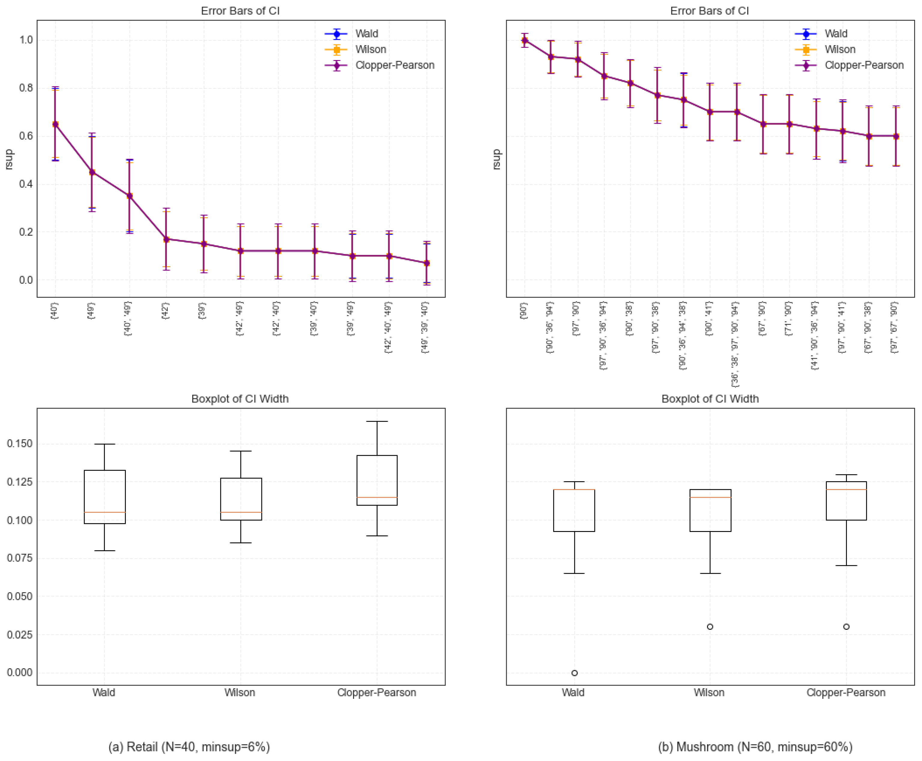
The relative support (rsup) error bars and boxplots of the Wald, Wilson, and Clopper–Pearson CI methods on the retail and mushroom datasets are presented in Figure 4. From the error bars, it can be observed that, compared with the Wald and Wilson methods, the Clopper–Pearson method exhibits a methodological conservatism on the two datasets, characterized by wider confidence intervals to ensure a higher coverage probability. In particular, the Wilson CI with a narrower confidence interval width shows marginally superior performance at specific data points. By analyzing the boxplots, it is determined that the overall distributions of the confidence interval widths of Wald and Wilson are similar, but the width of the Wilson method is slightly smaller than that of the Wald method, indicating that the Wilson CI is more compact and robust against sampling variety. However, the Clopper–Pearson method produces a larger CI width to accommodate the ubiquity of sample characteristics. Obviously, under various data distributions, the performance of distinct confidence interval methods differs. Therefore, it is very important to select a suitable confidence interval method in frequent pattern mining.
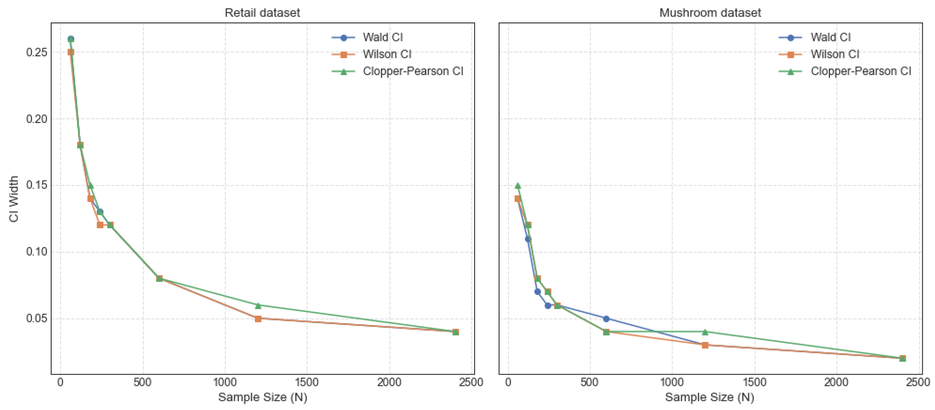
The trends of the CI width with sample size for the CFIs {‘40’} on the retail dataset and {‘97’, ‘90’} on the mushroom dataset are shown in Figure 5. It can be observed that the CI width of {‘97’, ‘90’} remains consistently narrower than that of {‘40’} with various sample sizes. This is because the mushroom dataset has a higher density than the retail dataset, which is more sparse. The Wald, Wilson, and Clopper–Pearson confidence intervals demonstrate progressively narrower widths as the sample size increases, indicating enhanced precision in the estimation of these intervals. There is no doubt that the distribution is closer to normality with the larger sample size and higher reliability. However, obtaining large datasets in real scenarios remains challenging. This emphasizes the significance of small sample conditions, which are crucial for the robust inference of population parameters. In this study, the integration of CFIs with three CI methods enhances the stability and reliability of frequent itemset mining, facilitating a more objective analysis of potential itemsets.
4. Conclusions and Future Work

Closed frequent itemset mining is applicable in various domains, e.g., healthcare, retail, and recommendation systems. In the past, most researchers focused on the improvement of algorithms rather than on the exploration of their properties. To strengthen the comprehensive understanding of the theoretical properties of CFIs, a series of theorems are systematically established, along with rigorous proofs. Furthermore, the concept of CICFIs and three distinct confidence interval estimation methods are presented to evaluate the stability of CFIs. Comprehensive experiments on an example dataset and two real datasets are conducted to further verify the theoretical properties, and the results show that the CICFIs and three distinct CI methods play significant roles in improving the reliability of practical applications. If a closed frequent itemset with high support falls within a narrow confidence interval, it suggests that the itemset is both frequent and stable in the dataset. In contrast, if the confidence interval is wide, the itemset is likely to be unstable and may represent a pseudo-frequent pattern caused by data variability. Such frequent and stable itemsets are valuable for supporting reliable decision-making in store operations, including inventory control and product promotion strategies. These contributions not only reinforce the theoretical foundation of CFIs but also facilitate the development of more efficient and robust algorithms for frequent pattern mining.
In the big data era, huge and various datasets are expanding rapidly. Faced with the problems of new transactions adding to and resulting in large datasets, re-mining the whole updated dataset is impractical and costly. Although some algorithms for large-scale databases [21,22], incremental databases [23,24], and dynamic databases [25,26] have been proposed, several promising directions can be further explored in the future, such as optimizing algorithms for mining CFIs to enhance scalability in large-scale and high-dimensional datasets, integrating closed frequent itemset mining with deep learning frameworks for more valuable knowledge discovery, and extending closed frequent itemset mining algorithms to dynamic datasets for the adaptation of incremental update strategies. By advancing these research directions, the applicability and efficiency of closed frequent itemset mining can be well expanded, reinforcing its role in large-scale data analysis and real-world decision-making systems.

Author Contributions

Conceptualization and methodology, H.Z. and H.L.; software and validation, H.Z. and Y.L.; writing—original draft preparation, H.Z.; writing—review and editing, H.L. and G.T.; supervision, G.T., Y.L. and X.C.; funding acquisition, X.C. All authors have read and agreed to the published version of the manuscript.

Funding

The research was supported by the National Natural Science Foundation of China under Grant number 62427811.

Data Availability Statement

Data are available in a publicly accessible repository.

Acknowledgments

We sincerely thank the anonymous reviewers for their valuable suggestions, which greatly strengthened our manuscript in various aspects.

Conflicts of Interest

The authors declare no conflicts of interest.

References

  1. Vimieiro, R.; Moscato, P. Disclosed: An efficient depth-first, top-down algorithm for mining disjunctive closed itemsets in high-dimensional data. Inf. Sci. 2014, 280, 171–187. [Google Scholar] [CrossRef]
  2. Dhanaseelan, R.; Sutha, M.J. Diagnosis of coronary artery disease using an efficient hash table based closed frequent itemsets mining. Med. Biol. Eng. Comput. 2018, 56, 749–759. [Google Scholar] [CrossRef] [PubMed]
  3. Kumar, P.M.; Rao, P.S. Mining closed high utility itemsets using sliding window infrastructure model over data stream. Int. J. Crit. Infrastructures 2024, 20, 447–462. [Google Scholar] [CrossRef]
  4. Kunjachan, H.; Hareesh, M.J.; Sreedevi, K.M. Recommendation using Frequent Itemset Mining in Big Data. In Proceedings of the 2nd International Conference on Intelligent Computing and Control Systems (ICICCS), Madurai, India, 14–15 June 2018; pp. 561–566. [Google Scholar]
  5. Fu, H.G.; Nguifo, E.M. Mining frequent closed itemsets for large data. In Proceedings of the 3rd International Conference on Machine Learning and Applications (ICMLA), Louisville, KY, USA, 16–18 December 2004; pp. 328–335. [Google Scholar]
  6. Qiu, Y.; Lan, Y.-J. Mining frequent closed itemsets with one database scanning. In Proceedings of the 5th International Conference on Machine Learning and Cybernetics, Dalian, China, 13–16 August 2006; pp. 1326–1331. [Google Scholar]
  7. Bay, V. An Efficient Method for Mining Frequent Weighted Closed Itemsets from Weighted Item Transaction Databases. J. Inf. Sci. Eng. 2017, 33, 199–216. [Google Scholar]
  8. Aryabarzan, N.; Minaei-Bidgoli, B. NECLATCLOSED: A vertical algorithm for mining frequent closed itemsets. Expert Syst. Appl. 2021, 174, 114738. [Google Scholar] [CrossRef]
  9. Wu, C.-W.; Huang, J.; Lin, Y.-W.; Chuang, C.-Y.; Tseng, Y.-C. Efficient algorithms for deriving complete frequent itemsets from frequent closed itemsets. Appl. Intell. 2022, 52, 7002–7023. [Google Scholar] [CrossRef]
  10. Liu, J.; Ye, Z.; Yang, X.; Wang, X.; Shen, L.; Jiang, X. Efficient strategies for incremental mining of frequent closed itemsets over data streams. Expert Syst. Appl. 2022, 191, 116220. [Google Scholar] [CrossRef]
  11. Ledmi, M.; Zidat, S.; Hamdi-Cherif, A. GrAFCI+ A fast generator-based algorithm for mining frequent closed itemsets. Knowl. Inf. Syst. 2021, 63, 1873–1908. [Google Scholar] [CrossRef]
  12. Mofid, A.H.; Daneshpour, N.; Torabi, Z. MMC: Efficient and effective closed high-utility itemset mining. J. Supercomput. 2024, 80, 18900–18918. [Google Scholar] [CrossRef]
  13. Agrawal, R.; Srikant, R. Fast algorithms for mining association rules. In Proceedings of the 20th International Conference on Very Large Data Bases (VLDB), Santiago de Chile, Chile, 12–15 September 1994; pp. 487–499. [Google Scholar]
  14. Pasquier, N.; Bastide, Y.; Taouil, R.; Lakhal, L. Discovering Frequent Closed Itemsets for Association Rules. In Database Theory—ICDT’99: 7th International Conference, Jerusalem, Israel, 10–12 January, 1999, Proceedings; Springer: Berlin/Heidelberg, Germany, 1999; pp. 398–416. [Google Scholar]
  15. Zaki, M.J.; Hsiao, C.-J. CHARM: An efficient algorithm for closed association rule mining. In Proceedings of the SIAM International Conference on Data Mining, Arlington, VA, USA, 11–13 April 2002. [Google Scholar]
  16. Zaki, M.J. Scalable algorithms for association mining. IEEE Trans. Knowl. Data Eng. 2000, 12, 372–390. [Google Scholar] [CrossRef]
  17. Ganter, B.; Wille, R. Formal Concept Analysis: Mathematical Foundations; Springer: Berlin/Heidelberg, Germany, 1997. [Google Scholar]
  18. Han, J.; Pei, J.; Kamber, M. Data Mining: Concepts and Techniques, 3rd ed.; Morgan Kaufmann: San Francisco, CA, USA, 2011. [Google Scholar]
  19. Zhou, P.; Wei, H.; Zhang, H. Selective Reviews of Bandit Problems in AI via a Statistical View. Mathematics 2025, 13, 665. [Google Scholar] [CrossRef]
  20. Fournier-Viger, P.G.A.; Gueniche, T.; Soltani, A.; Wu, C.W.; Tseng, V.S. SPMF: A Java open-source pattern mining library. J. Mach. Learn. Res. 2014, 15, 3389–3393. [Google Scholar]
  21. Lin, J.C.-W.; Djenouri, Y.; Srivastava, G. Efficient closed high-utility pattern fusion model in large-scale databases. Inf. Fusion 2021, 76, 122–132. [Google Scholar] [CrossRef]
  22. Lin, J.C.-W.; Djenouri, Y.; Srivastava, G.; Wu, J.M.-T. Large-Scale Closed High-Utility Itemset Mining. In Proceedings of the 21st IEEE International Conference on Data Mining (IEEE ICDM), Auckland, New Zealand, 7–10 December 2021; pp. 591–598. [Google Scholar]
  23. Magdy, M.; Ghaleb, F.F.M.; Mohamed, D.A.E.A.; Zakaria, W. CC-IFIM: An efficient approach for incremental frequent itemset mining based on closed candidates. J. Supercomput. 2023, 79, 7877–7899. [Google Scholar] [CrossRef]
  24. Al-Zeiadi, M.A.; Al-Maqaleh, B.M. Incremental Closed Frequent Itemsets Mining-Based Approach Using Maximal Candidates. IEEE Access 2025, 13, 34023–34037. [Google Scholar] [CrossRef]
  25. Cai, J.; Chen, Z.; Chen, G.; Gan, W.; Broustet, A. Periodic frequent subgraph mining in dynamic graphs. Int. J. Mach. Learn. Cybern. 2025. [Google Scholar] [CrossRef]
  26. Nguyen, T.D.D.; Nguyen, L.T.T.; Vu, L.; Vo, B.; Pedrycz, W. Efficient algorithms for mining closed high utility itemsets in dynamic profit databases. Expert Syst. Appl. 2021, 186, 115741. [Google Scholar] [CrossRef]
Figure 1. CI width comparison on the example dataset.
Mathematics 13 01709 g001
Figure 2. CI width comparison on retail dataset.
Mathematics 13 01709 g002
Figure 3. CI width comparison with top ten CFIs on mushroom dataset.
Mathematics 13 01709 g003
Figure 4. The rsup error bars and boxplot of CI width.
Mathematics 13 01709 g004
Figure 5. The trend of CI width with sample size.
Mathematics 13 01709 g005
Table 1. A sample dataset.
TidsItems
t 1 A B D E
t 2 B C E
t 3 A B C E
t 4 A B E
t 5 A B C D E
t 6 B C D
t 7 B C D E
Table 2. FIs (minsup = 4).
supFIs
7B
6E, BE
5C, BC
4A, D, AB, AE, BD, CE, ABE, BCE
Table 3. The equivalent class, closure, and Tids on FIs.
Equivalent ClassClosureTids
A, AB, AE, ABEABE t 1 , t 3 , t 4 , t 5
BB t 1 , t 2 , t 3 , t 4 , t 5 , t 6 , t 7
C, BCBC t 2 , t 3 , t 5 , t 6 , t 7
CE, BCEBCE t 2 , t 3 , t 5 , t 7
D, BDBD t 1 , t 5 , t 6 , t 7
E, BEBE t 1 , t 2 , t 3 , t 4 , t 5 , t 7
Table 4. The characteristics of two real datasets.
DatasetsTransactionsItemsAvg.Trans.LenMax.Trans.LenType
retail88,16216,40710.376Sparse
mushroom81241192323Dense
Table 5. The results of three distinct CI methods of CFIs on the example dataset.
CFIssuprsupWald CIWidth1Wilson CIWidth2Clopper–Pearson CIWidth3
{‘B’}71.00(1.00, 1.00)0.00(0.65, 1.00)0.35(0.59, 1.00)0.41
{‘B’, ‘E’}60.86(0.60, 1.00)0.40(0.49, 0.97)0.48(0.42, 1.00)0.58
{‘C’, ‘B’}50.71(0.38, 1.00)0.62(0.36, 0.92)0.56(0.29, 0.96)0.67
{‘D’, ‘B’}40.57(0.20, 0.94)0.74(0.25, 0.84)0.58(0.18, 0.90)0.72
{‘B’, ‘E’, ‘A’}40.57(0.20, 1.00)0.74(0.25, 0.84)0.59(0.18, 0.90)0.72
{‘C’, ‘B’, ‘E’}40.57(0.20, 0.90)0.74(0.25, 0.84)0.59(0.18, 0.90)0.72
Table 6. The results of three distinct CI methods of CFIs on retail dataset.
CFIssuprsupWald CIWidth1Wilson CIWidth2Clopper–Pearson CIWidth3
{‘40’}260.65(0.50, 0.80)0.30(0.50, 0.78)0.28(0.48, 0.79)0.31
{‘49’}180.45(0.30, 0.60)0.30(0.31, 0.60)0.29(0.29, 0.62)0.33
{‘40’, ‘49’}140.35(0.20, 0.50)0.30(0.22, 0.50)0.28(0.21, 0.52)0.31
{‘42’}70.17(0.06, 0.29)0.23(0.09, 0.32)0.23(0.07, 0.33)0.26
{‘39’}60.15(0.04, 0.26)0.22(0.07, 0.29)0.22(0.06, 0.30)0.24
{‘42’, ‘49’}50.12(0.02, 0.23)0.21(0.05, 0.26)0.21(0.04, 0.27)0.23
{‘42’, ‘40’}50.12(0.02, 0.23)0.21(0.05, 0.26)0.21(0.04, 0.27)0.23
{‘39’, ‘40’}50.12(0.02, 0.23)0.21(0.05, 0.26)0.21(0.04, 0.27)0.23
{‘39’, ‘49’}40.10(0.01, 0.19)0.18(0.04, 0.23)0.19(0.03, 0.24)0.21
{‘42’, ‘40’, ‘49’}40.10(0.01, 0.19)0.18(0.04, 0.23)0.19(0.03, 0.24)0.21
{‘49’, ‘39’, ‘40’}30.07(0.00, 0.16)0.16(0.03, 0.20)0.17(0.02, 0.20)0.18
Table 7. The results of three distinct CI methods of CFIs on mushroom dataset.
CFIssuprsupWald CIWidth1Wilson CIWidth2Clopper–Pearson CIWidth3
{‘90’}601.00(1.00, 1.00)0.00(0.94, 1.00)0.06(0.94, 1.00)0.06
{‘90’, ‘36’, ‘94’}590.98(0.95, 1.00)0.05(0.91, 1.00)0.09(0.91, 1.00)0.09
{‘97’, ‘90’}550.92(0.85, 0.99)0.14(0.82, 0.96)0.14(0.82, 0.97)0.15
{‘97’, ‘90’, ‘36’, ‘94’}540.90(0.82, 0.98)0.16(0.80, 0.95)0.15(0.79, 0.96)0.17
{‘90’, ‘38’}520.87(0.78, 0.95)0.17(0.76, 0.93)0.17(0.75, 0.94)0.19
{‘90’, ‘36’, ‘94’, ‘38’}510.85(0.76, 0.94)0.18(0.74, 0.92)0.18(0.73, 0.93)0.20
{‘97’, ‘90’, ‘38’}490.82(0.72, 0.91)0.19(0.70, 0.89)0.19(0.70, 0.90)0.20
{‘36’, ‘38’, ‘97’, ‘90’, ‘94’}480.80(0.70, 0.90)0.20(0.68, 0.88)0.20(0.68, 0.89)0.21
{‘67’, ‘90’}390.65(0.53, 0.77)0.24(0.52, 0.76)0.24(0.52, 0.77)0.25
{‘90’, ‘41’}380.63(0.51, 0.76)0.25(0.51, 0.74)0.23(0.50, 0.75)0.25
{‘90’, ‘24’}380.63(0.51, 0.76)0.25(0.51, 0.74)0.23(0.50, 0.75)0.25
{‘67’, ‘90’, ‘36’, ‘94’}380.63(0.51, 0.76)0.25(0.51, 0.74)0.23(0.50, 0.75)0.25
{‘41’, ‘90’, ‘36’, ‘94’}370.62(0.49, 0.74)0.25(0.49, 0.73)0.24(0.48, 0.74)0.26
{‘90’, ‘36’, ‘94’, ‘2’}370.62(0.49, 0.74)0.25(0.49, 0.73)0.24(0.48, 0.74)0.26
{‘90’, ‘36’, ‘94’, ‘24’}370.62(0.49, 0.74)0.25(0.49, 0.73)0.24(0.48, 0.74)0.26
{‘97’, ‘90’, ‘24’}360.60(0.48, 0.72)0.24(0.47, 0.71)0.24(0.47, 0.72)0.25
{‘36’, ‘97’, ‘90’, ‘2’, ‘94’}360.60(0.48, 0.72)0.24(0.47, 0.71)0.24(0.47, 0.72)0.25
Disclaimer/Publisher’s Note: The statements, opinions and data contained in all publications are solely those of the individual author(s) and contributor(s) and not of MDPI and/or the editor(s). MDPI and/or the editor(s) disclaim responsibility for any injury to people or property resulting from any ideas, methods, instructions or products referred to in the content.