Two-Dimensional Fluid Flow Due to Blade-Shaped Waving of Cilia in Human Lungs

Abstract

The mucociliary clearance system is an innate defense mechanism in the human respiratory tract, which plays a crucial role in protecting the airways from infections. The clearance system secretes mucus from the goblet cells, which scatters in the respiratory epithelium to trap foreign particles entering the airway, and then the mucus is removed from the body via the movement of cilia residing under the mucus and above the epithelium cells. The layer containing cilia is called the periciliary layer (PCL). This layer also contains an incompressible Newtonian fluid called PCL fluid. This study aims to determine the velocity of the PCL fluid driven by the cilia movement instead of a pressure gradient. We consider bundles of cilia, rather than an individual cilium. So, the generalized Brinkman equation in a macroscopic scale is used to predict the fluid velocity in the PCL. We apply a mixed finite element method to the governing equation and calculate the numerical solutions in a two-dimensional domain. The numerical domain is set up to be the shape of a fan blade, which is similar to the motion of the cilia. This problem can be applied to problems of fluid flow propelled via moving solid phases.

1. Introduction

Cilia are hair-like structures located on the surfaces of many organisms, such as Paramecium, amoeba, and complex multicellular organisms. The human body contains numerous cilia that can be found both inside the body and on the human skin. Cilia, for example, help move eggs through the fallopian tubes into the uterus and move sperm in the reproductive system [1]. Cilia help pass food and waste through the digestive tract [2]. They also aid digestion and prevent intestine blockages [2]. Cilia in the respiratory system help move mucus and foreign particles out of the lungs and airways [3]. They are self-propelled structures that move in a way called metachronal motion. This protects the lungs and respiratory system from infection. This research focuses on the cilia found in the innate immune system in the human respiratory system, which play an important role in protecting the body from small particles contaminated with inhaled air, such as dust.

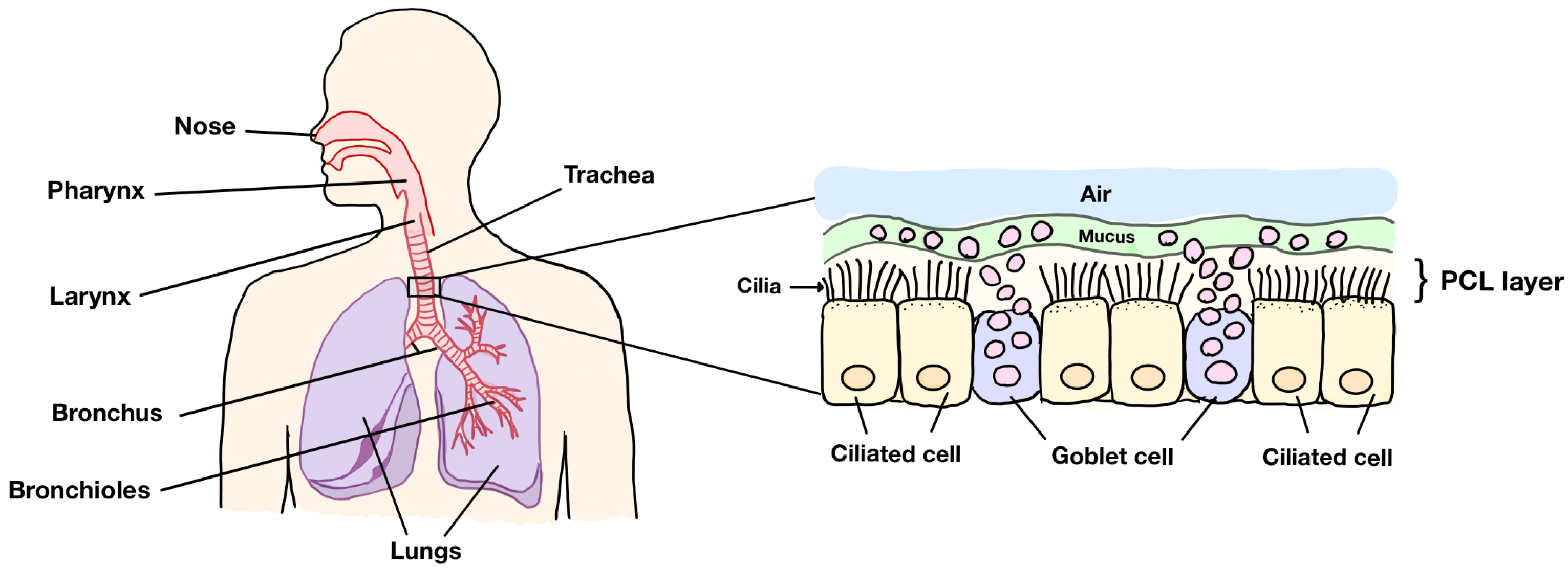
Figure 1 illustrates the human respiratory system (left) and a portion of the trachea in the respiratory tract (right). The system consists of the nose, pharynx, larynx, trachea, bronchus, bronchioles, and lungs. When closely inspecting the trachea, we can see that there are three main layers in the right figure: the periciliary layer (PCL), the mucus region, and the air at the top layer. In the respiratory tract, cilia are found in the PCL. The PCL also contains fluid that is considered to be an incompressible Newtonian fluid because the PCL fluid is a fluid similar to water in its properties, such as viscosity [4]. The fluid in this layer is called PCL fluid. The area under the PCL is comprised of goblet cells scattering among the ciliated cells. The ciliated cell is the cell membrane where the cilia reside on the top of the cell. The goblet cells contain mucus granules, which secrete mucus to trap strange particles entering the human body. After capturing foreign particles, mucus forms a layer at the tips of cilia. To prevent the accumulation of mucus in the lungs, cilia beat forward and backward producing metachronal waves, which fully expand during the forward stroke and then bend close to the epithelium before rotating back to the beginning of the forward stroke to push mucus out of the lungs. This system is known as mucociliary clearance in human lungs. Above the mucus layer is the air row, which is the path for bringing oxygen in and sending carbon dioxide out of the body. In this research, we focus on the velocity of the fluid in the PCL moved via the movement of cilia, rather than a pressure gradient. Since the PCL consists of both solid phases (cilia) and the liquid phase (the PCL fluid) and the PCL has interconnected pores through which fluids can move, which is the characteristic of a porous medium, we consider the PCL a porous medium.

Problems of the PCL have been studied by several researchers [5,6,7,8,9,10,11,12,13,14]. For example, Zhu et al. [5] proposed a two-dimensional model to explore the migration law of particles due to cilium beat in the PCL of the human respiratory tract using the immersed boundary-lattice Boltzmann method. Poopra and Wuttanachamsri [6] provide boundary conditions at the top of the PCL due to the ciliary movement. Vanaki et al. [7] studied the fluid flow in the PCL driven by cilia using the finite difference method and the immersed boundary method. Jayathilake et al. [8] developed a three-dimensional numerical model to simulate human pulmonary cilia motion in the PCL and investigated the effects of the phase difference between cilia, the cilia beating frequency, the viscosity of PCL, the PCL height, and the ciliary length affecting the PCL fluid motion. Phaenchat and Wuttanachamsri [14] determined the velocity of the PCL fluid in a two-dimensional domain. They used the nonlinear Brinkman equation in the porous medium. The equation was solved using a mixed finite element method combined with Newton’s method.

Many researchers have studied the fluid flow through porous domains using the Brinkman equation both analytically and numerically. For example, analytical studies focused on proving the well-posedness of the equation [15,16,17,18,19,20,21]. Conti and Giorgini [15] proved the existence and uniqueness of the Brinkman–Cahn–Hilliard system with logarithmic free energy density for the motion of binary fluids with different viscosities. Titi and Trabelsi [16] derived the existence and uniqueness of a three-dimensional Brinkman–Forchheimer–Bénard convection model for an incompressible fluid in a closed sample of a porous medium. For numerical solutions of the Brinkman equation, they were studied by several researchers [22,23,24,25,26,27,28,29,30,31] in many aspects. For example, Wuttanachamsri [23] observed the velocity of the PCL fluid and the shape of the free boundary at the tips of cilia when the fluid was driven via cilia movement using a one-dimensional Brinkman equation with the Stefan problem. Basirat et al. [24] predicted the flow and transport of gaseous CO₂ in a porous medium using the Darcy–Brinkman equation with COMSOL software based on the finite element method. Wuttanachamsri and Schreyer [25] applied a mixed finite element method of the Taylor–Hood type to the Stokes–Brinkman equations to find the PCL fluid velocities due to the cilia beating in a three-dimensional domain. Nishad et al. [26] proposed a new Boundary Integral Equation (BIE) method and also investigated the two-dimensional Brinkman flow of incompressible Newtonian fluids through a porous channel. Cortez et al. [28] provided the exact and numerical solutions for the Brinkman equation in a three-dimensional domain where the incompressible flow was driven by regularized forces. Kanafiah et al. [30] investigated the numerical results of the Brinkman–viscoelastic fluid model for mixed convection transport via a horizontal circular cylinder saturated in a porous domain. Pranowo and Wijayanta [31] proposed the numerical solutions of the Darcy–Brinkman–Forchheimer model for forced–convective fluid flow in a porous medium using the Direct Meshless Local Petrov–Galerkin (DMLPG) method. Most of the previous literature had studied the numerical solutions of the Brinkman equation when the fluid moved by the pressure gradient. 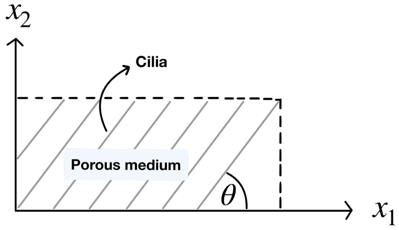Although some works [6,11,12,14,23,25] considered the fluid velocity due to the movement of the solid phases, they assumed that the porosity was a constant, and they calculated the numerical results for a fixed angle $\theta$ on a rectangular domain, as shown in Figure 2.

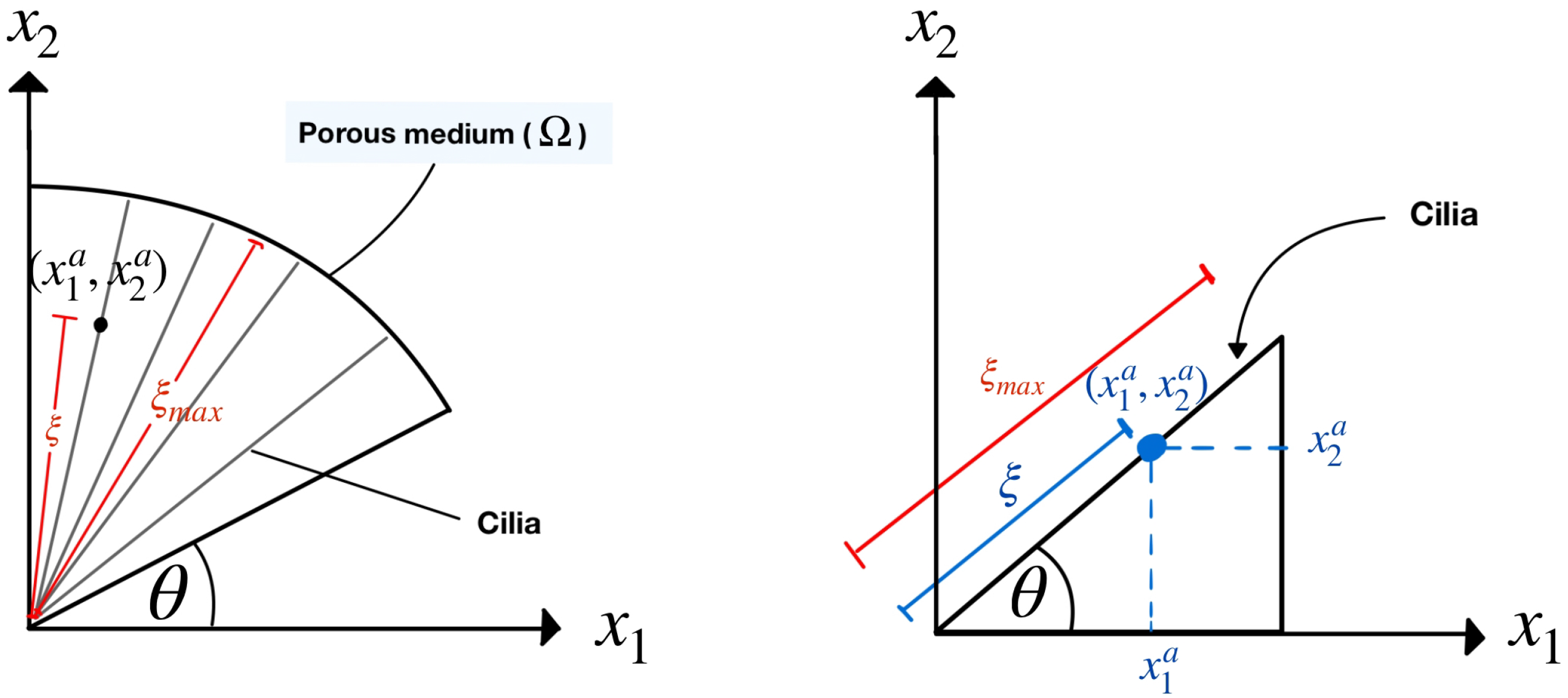
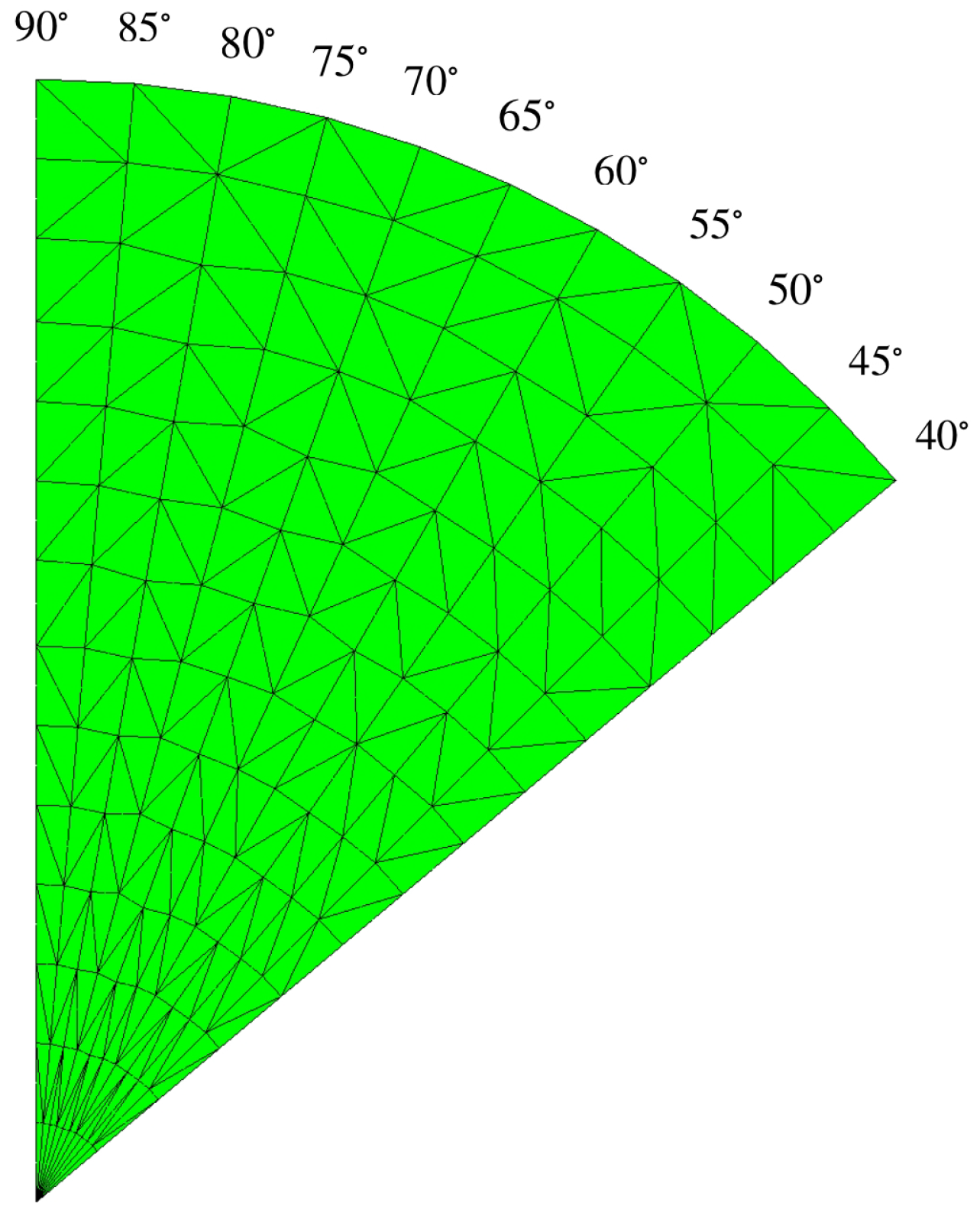
Figure 2 illustrates a rectangular porous domain composed of cilia that make an angle $\theta$ with the horizontal plane. In fact, the angle $\theta$ and the porosity should be varied in the numerical domain because of the metachronal waves of cilia. Unlike the other researchers, in this work, we define the numerical domain in the shape of a fan blade, resembling the wave pattern of cilia, as shown on the left side of Figure 3, where the cilia are monitored as rigid cylinders because they have long and thin lines. Based on our information, this shape of the domain was not studied in the previous literature. The model designed is more closely to the actual beating pattern of cilia in that the cilia rotate as a clockwise pattern moving from left to right around their base. The movement of cilia generates the leftward flow of the PCL fluid. Figure 3 on the left shows our numerical porous domain with the angular movement of the cilia. The angle $\theta$ represents the angle that the cilia make with the horizontal plane. In previous research, scholars have not studied various angles, $\theta$, in one fixed numerical domain. They considered only one angle, $\theta$, for one fixed numerical domain. Notice that there are numerous angles, $\theta$, in our one fixed numerical domain. Since there are several angles, $\theta$, in the domain, the porosity cannot be used as a constant. So, the porosity in this work is considered a function of the angle, $\theta$, not a constant. The variable $\xi$ is the dimensionless length along cilia, which is the distance from the roots of the cilia to a point $(x_1^a,x_2^a)$ on the cilia divided by the length of the cilia, which is approximately 7.5 µm [32]. Figure 3 on the right shows that, at each point $(x_1^a,x_2^a)$ on the cilia, we can calculate the variable $\xi$ using the formula $\xi =x_2^a/sin\theta$ and the angle $\theta =arctan(x_2^a/x_1^a)$, and the variable ${\xi }_{\max }$ represents the dimensionless length of the cilia, which is one. Because we consider the movement of bundles of cilia affecting the movement of the PCL fluid, we use the generalized Brinkman equation [33] on a macroscopic scale to predict the velocity of the PCL fluid in the porous medium. The mathematical model we use is derived in [33], which is a macroscale equation determined from an upscaling technique called Hybrid Mixture Theory (HMT) [34,35,36] and the nondimensionalization method. This model is more general than the Brinkman equation in the literature because we choose to use the equation that the porosity in this equation is considered as a function since the beginning of the derivation starting from the conservation of momentum. The generalized Brinkman equation is not only derived in [33] but the authors have also proved the existence and uniqueness of the numerical solution when the equation is applied via a mixed finite element method. In [33], the authors used the Lax–Milgram theorem to prove the well-posedness of the equation. To the author’s knowledge, the generalized Brinkman equation was not solved numerically in any literature before. It is solved for the first time in this work. The aim of this research is to determine the velocity of the PCL fluid in the fan-blade shape of the porous domain using the generalized Brinkman equation, in which the fluid is driven by the beating of cilia.

Our mathematical model and boundary conditions are provided in Section 2. To determine the numerical solutions, we discretize the governing equation by using a mixed finite element method in Section 3. The velocity of cilia, permeability, and porosity are described in Section 4. The validation of the numerical solutions is presented in Section 5, and the numerical results are illustrated in Section 6. The validation and numerical results are computed from our own code using MatLab R2025a. The conclusions are drawn in Section 7.

2. Mathematical Model and Boundary Conditions

Because we consider the movement of a bundle of self-propelled cilia, rather than a single cilium in the fan-blade shape of the porous medium, the generalized Brinkman equation on the macroscopic scale is employed as our governing equation, which is shown in Section 2.1, and the boundary conditions are illustrated in Section 2.2.

2.1. Governing Equations

The mathematical model employed in this work is the generalized Brinkman equation on the macroscopic scale. The derivation of this equation has been proven in [33] using the Hybrid Mixture Theory (HMT) [34,35,36]. HMT is an upscaling technique that the averaging theorem is used to upscale equations from a microscale equation to a macroscale equation. For example, consider the conservation of mass equation at the microscale,

$${\displaystyle \frac{\partial \rho }{\partial t}}+\nabla ·\left(\rho \mathbf{v}\right)=0,$$

(1)

where $\rho$ is the density, t is time, and $\mathbf{v}$ is the velocity. Multiplying Equation (1) by an indicator function for phase $\alpha ,{\gamma }_{\alpha }$, and then integrating the equation over a representative elementary volume (REV) and applying the averaging theorem [34,35],

$${\displaystyle \frac{1}{\left|\delta V\right|}{\int }_{\delta V}\frac{\partial F}{\partial t}{\gamma }_{\alpha }dv\left(\xi \right)=\frac{\partial }{\partial t}\left[\frac{1}{\left|\delta V\right|}{\int }_{\delta V}F{\gamma }_{\alpha }dv\left(\xi \right)\right]-\sum _{\beta \ne \alpha }\frac{1}{\left|\delta V\right|}{\int }_{\delta A_{\alpha \beta }}F{\mathbf{w}}_{\alpha \beta }·{\mathbf{n}}_{\alpha }da\left(\xi \right),}$$

(2)

$${\displaystyle \frac{1}{\left|\delta V\right|}}{\int }_{\delta V}{\nabla }_{x}F{\gamma }_{\alpha }dv\left(\xi \right)={\nabla }_x\left[{\displaystyle \frac{1}{\left|\delta V\right|}}{\int }_{\delta V}F{\gamma }_{\alpha }dv\left(\xi \right)\right]+\sum _{\beta \ne \alpha }{\displaystyle \frac{1}{\left|\delta V\right|}}{\int }_{\delta A_{\delta \beta }}F{\mathbf{n}}_{\alpha }da\left(\xi \right),$$

(3)

to the integral equation, we have

$$\begin{array}{c}\hfill {\displaystyle \frac{\partial \left({\epsilon }^{\alpha }{\rho }^{\alpha }\right)}{\partial t}}+\nabla ·\left({\epsilon }^{\alpha }{\rho }^{\alpha }{\mathbf{v}}^{\alpha }\right)=\sum _{\beta \ne \alpha }{\epsilon }^{\alpha }{\rho }^{\alpha }{\widehat{e}}_{\beta }^{\alpha },\end{array}$$

(4)

which is the macroscale conservation of mass. Here, $\delta V$ denotes the representative elementary volume (REV), $\left|\delta V\right|$ is the magnitude of REV, F is the quantities in the field equations, $\delta A_{\alpha \beta }$ is the portion of the $\alpha \beta$ interface within $\delta V$, ${\mathbf{w}}_{\alpha \beta }$ is the microscopic velocity of interface $\alpha \beta$, and ${\mathbf{n}}_{\alpha }$ is the outward unit normal vector to $\delta V_{\alpha }$. The variable ${\rho }^{\alpha }$ is the macroscale density of phase $\alpha$, ${\mathbf{v}}^{\alpha }$ is the macroscale velocity of phase $\alpha$, ${\widehat{e}}_{\beta }^{\alpha }$ is the rate of exchange of mass from phase $\beta$ to phase $\alpha$, and ${\epsilon }^{\alpha }$ is the volume fraction of phase $\alpha$.

Next, we briefly show the derivation of the generalized Brinkman equation [33]. We start with the multiphase equation [37], which is upscaled from the conservation of momentum using HMT when the porosity is a function. That is,

$${\displaystyle {\epsilon }^l\rho \frac{D^l{\mathbf{u}}^l}{Dt}+{\epsilon }^l\nabla p+p\nabla {\epsilon }^l-\nabla ·\left({\epsilon }^{l}2\mu {\mathbf{d}}^l\right)-{\epsilon }^l\rho \mathbf{g}=p\nabla {\epsilon }^l-{\epsilon }^l\mathbf{R}·({\mathbf{u}}^l-{\mathbf{u}}^s),}$$

(5)

where the variables l and s mean the liquid and solid phases, respectively. The function ${\epsilon }^l$ is the porosity, which is a variable in space, ${\mathbf{u}}^l$ and ${\mathbf{u}}^s$ are the velocities of the PCL fluid and solid phases (cilia), respectively, p is the pressure, $\mu$ is the dynamic viscosity, ${\mathbf{d}}^l=0.5\left(\nabla {\mathbf{u}}^l+{(\nabla {\mathbf{u}}^l)}^T\right)$ is the rate of deformation tensor, $\mathbf{g}$ is the gravity, and $\mathbf{R}$ is a second-order tensor. Subtracting $p\nabla {\epsilon }^l$ from both sides in Equation (5), dividing both sides by ${\epsilon }^l$, substituting ${\displaystyle \frac{D^l{\mathbf{u}}^l}{Dt}=\frac{\partial {\mathbf{u}}^l}{\partial t}+{\mathbf{u}}^l·\nabla {\mathbf{u}}^l}$, which is the definition of the material time derivative for liquid phase [37], taking $\mathbf{R}=\mu {\epsilon }^l{\mathbf{k}}^{-1}$, where ${\mathbf{k}}^{-1}$ is the inverse of the permeability tensor, and then rearranging the terms, we have

$${\displaystyle \rho \left({\displaystyle \frac{\partial {\mathbf{u}}^l}{\partial t}+{\mathbf{u}}^l·\nabla {\mathbf{u}}^l}\right)+\mu {\mathbf{k}}^{-1}·({\epsilon }^l{\mathbf{u}}^l-{\epsilon }^l{\mathbf{u}}^s)+\nabla p-\frac{\mu }{{\epsilon }^l}\nabla ·\left(2{\epsilon }^l{\mathbf{d}}^l\right)=\rho \mathbf{g},}$$

(6)

which is the conservation of momentum for the liquid phase. After that, the Equation (6) is normalized with dimensionless variables. So, some terms are neglected. Then, Equation (6) becomes

$${\displaystyle \mu {\mathbf{k}}^{-1}·({\epsilon }^l{\mathbf{u}}^l-{\epsilon }^l{\mathbf{u}}^s)+\nabla p-\frac{\mu }{{\epsilon }^l}\nabla ·\left(2{\epsilon }^l{\mathbf{d}}^l\right)=\rho \mathbf{g},}$$

(7)

which is called the generalized Brinkman equation in a macroscopic scale.

Let $\mathrm{\Omega }$ be the domain of the porous medium and $\mathrm{\Gamma }$ be the boundary of the domain $\mathrm{\Omega }$. The generalized Brinkman equation, Equation (7), and the continuity equation [38] used in the PCL are

$$\begin{array}{cccc}\hfill \mu {\mathbf{k}}^{-1}·\left({\epsilon }^l{\mathbf{u}}^l\right)-{\displaystyle \frac{\mu }{{\epsilon }^l}}\nabla ·\left(2{\epsilon }^l{\mathbf{d}}^l\right)+\nabla p& =\rho \mathbf{g}+\mu {\mathbf{k}}^{-1}·\left({\epsilon }^l{\mathbf{u}}^s\right),\hfill & \hfill & \mathrm{in}\mathrm{\Omega }\hfill \end{array}$$

(8)

$$\begin{array}{cccc}\hfill \nabla ·\left({\epsilon }^l{\mathbf{u}}^l\right)& =f,\hfill & \hfill & \hfill \mathrm{in}\mathrm{\Omega }\end{array}$$

(9)

where $f={\dot{\epsilon }}^l/\left(1-{\epsilon }^l\right)+\nabla ·\left({\epsilon }^l{\mathbf{u}}^s\right)$ and ${\dot{\epsilon }}^l=\partial {\epsilon }^l/\partial t+{\mathbf{u}}^s·\nabla {\epsilon }^l$ is the material time derivative of the porosity with respect to the solid phase. Notice that the terms that have the inverse of the permeability in Equation (8) help in understanding the ability of the PCL fluid to flow through the PCL. The gravity term is the force exerted by Earth’s gravity on the PCL fluid within the PCL. The pressure term represents the impact of pressure on fluid flow. The rate of deformation term refers to the change in velocity in different directions. The function f in Equation (9) tracks the rate of change of the porosity with respect to time. This term helps in understanding the change in porosity as we move along with the cilia. Define the vector

$$\mathbf{u}={\epsilon }^l{\mathbf{u}}^l.$$

(10)

Substituting Equation (10) into Equations (8) and (9), we obtain the system of equations

$$\begin{array}{cccc}\hfill \mu {\mathbf{k}}^{-1}·\mathbf{u}-{\displaystyle \frac{\mu }{{\epsilon }^l}}\nabla ·\left(2{\epsilon }^l{\mathbf{d}}^l\right)+\nabla p& =\rho \mathbf{g}+\mu {\mathbf{k}}^{-1}·{\epsilon }^l{\mathbf{u}}^s,\hfill & \hfill & \mathrm{in}\mathrm{\Omega }\hfill \end{array}$$

(11)

$$\begin{array}{cccc}\hfill \nabla ·\mathbf{u}& =f,\hfill & \hfill & \mathrm{in}\mathrm{\Omega }\hfill \end{array}$$

(12)

which is used in this work. The unknowns of the system of equations are the fluid velocity, $\mathbf{u}$, and the pressure, p.

2.2. Boundary Conditions

In this work, we consider the forward stroke of cilia moving from the angle $\theta ={90}^{\circ }$ to ${40}^{\circ }$. The numerical domain and the boundaries are shown in Figure 4. The variable $x_1^b$ is the length at which ${\xi }_{\max }$ is projected on the $x_1$ axis when the cilia make the angle $\theta ={40}^{\circ }$ with the horizontal plane. Then, $x_1^b=cos{40}^{\circ }$ and $0\le x_2\le 1$. The variables ${\mathrm{\Gamma }}_i,i=1,2,3$ are the boundaries of the domain $\mathrm{\Omega }$ and $\mathrm{\Gamma }={\mathrm{\Gamma }}_1\cup {\mathrm{\Gamma }}_2\cup {\mathrm{\Gamma }}_3$. We let $\mathbf{u}=(u_1,u_2)$ be the velocity vector, where $u_1$ is the velocity in the rightward direction, and $u_2$ is the velocity in the upward direction, in which the velocity these directions are considered to be positive numbers. If the cilia move in the downward direction, the velocity $u_2$ becomes negative. At the boundary ${\mathrm{\Gamma }}_1$, we let the fluid velocity be equal to the velocity of the cilia, provided in Section 4, when the angle $\theta ={90}^{\circ }$. Since, from the experimental data, [39], the cilia move forward rapidly and stop moving at $\theta ={40}^{\circ }$, approximately before having the reverse movement, in this work, we assume that the velocity of the cilia is zero at $\theta ={40}^{\circ }$. So, the velocity at the boundary ${\mathrm{\Gamma }}_3$ is zero. For the boundary condition at ${\mathrm{\Gamma }}_2$, since no one really knows the condition at ${\mathrm{\Gamma }}_2$, we consider two cases for this problem.

Case 1: We employ the boundary conditions from [23], where they have determined the velocity at the tips of cilia when the cilia move forward and backward. They provide that the rate of change of the fluid velocities with respect to $x_1$ and $x_2$ depends on the exponential function of the angle $\theta$. So, our boundary conditions at ${\mathrm{\Gamma }}_1,{\mathrm{\Gamma }}_2$, and ${\mathrm{\Gamma }}_3$ are

$$\begin{array}{cccc}\hfill & u_1(0,x_2)=u^s\left(x_2\right),\hfill & \hfill & \mathrm{at}{\mathrm{\Gamma }}_1\hfill \end{array}$$

(13)

$$\begin{array}{cccc}\hfill & {\displaystyle \frac{\partial u_1}{\partial x_1}}=c_1{e}^{\theta },{\displaystyle \frac{\partial u_1}{\partial x_2}}=c_2{e}^{\theta },{\displaystyle \frac{\partial u_2}{\partial x_1}}=c_3{e}^{\theta },{\displaystyle \frac{\partial u_2}{\partial x_2}}=c_4{e}^{\theta },\hfill & \hfill & \mathrm{at}{\mathrm{\Gamma }}_2\hfill \end{array}$$

(14)

$$\begin{array}{cccc}\hfill & u_1(x_1,x_2)=u_2(x_1,x_2)=0,\hfill & \hfill & \mathrm{at}{\mathrm{\Gamma }}_3\hfill \end{array}$$

(15)

where $c_1,c_2,c_3$, and $c_4$ are constants.

The constants $c_i,i=1,2,3,4,$ can be positive, negative, or zero. It depends on the problems that one considers. For example, if $c_1=0$, then ${\displaystyle \frac{\partial u_1}{\partial x_1}}=0$. Therefore, the rate of change of $u_1$ with respect to $x_1$ is zero. That is, $u_1$ remains a constant even $x_1$ has been changed.

Case 2: We assume that boundary conditions at ${\mathrm{\Gamma }}_2$ are unknown. So, to obtain the numerical solution, the velocities $u_1$ and $u_2$ at ${\mathrm{\Gamma }}_2$ are moved to the left-hand side of the equation and used to find the numerical solution, in order to determine $u_1$ and $u_2$ at ${\mathrm{\Gamma }}_2$.

The governing equations, the generalized Brinkman equation, and the boundary conditions used in this work are now provided. Before we calculate the numerical results, we provide the discretized form of our mathematical model using a mixed finite element method in the next section.

3. Model Discretization

In this section, we discretize the system of equations, Equations (11) and (12) using a mixed finite element method. We begin with the generalized Brinkman equation in the indicial notation for two dimensions,

$$\mu k_{ij}^{-1}{u}_j-{\displaystyle \frac{\mu }{{\epsilon }^l}}{\displaystyle \frac{\partial }{\partial x_j}}\left(2{\epsilon }^l{d}_{ij}^l\right)+{\displaystyle \frac{\partial p}{\partial x_i}}=\rho g_i+\mu {\epsilon }^l{k}_{ij}^{-1}{u}_j^s,\mathrm{in}\mathrm{\Omega }$$

(16)

for $i,j=1,2$ and $(g_1,g_2)=\left(0,-g\right)$ where g is gravity. The index i indicates the number of equations, and the repeated index j indicates summation. Let $H^1\left(\mathrm{\Omega }\right)$ be the Hilbert space and $L_0^2\left(\mathrm{\Omega }\right)$ be the Sobolev space, defined as follows,

$$L_0^2\left(\mathrm{\Omega }\right)=\left\{q\in L^2\left(\mathrm{\Omega }\right):{\int }_{\mathrm{\Omega }}qd\mathrm{\Omega }=0\right\}\mathrm{and}{H}_0^1\left(\mathrm{\Omega }\right)=\left\{\mathbf{w}\in H^1\left(\mathrm{\Omega }\right):\mathbf{w}{|}_{\partial \mathrm{\Omega }}=0\right\}.$$

(17)

To find $\left(\mathbf{u},p\right)\in H^1\left(\mathrm{\Omega }\right)\times L_0^2\left(\mathrm{\Omega }\right)$, we first provide the weak formulation of Equation (16). The weak formulation is the lower-order integral equations obtained from multiplying the higher-order differential Equation (16) by a weight function and then integrating over the domain and after that applying the Green’s identity, which is integration by parts in one dimension, to the integral equation. To find the weak formulation, we multiply Equation (16) by a weight function, $w_i\in H_0^1\left(\mathrm{\Omega }\right)$, and then we integrate over the domain $\mathrm{\Omega }$ both sides. Therefore, the Equation (16) becomes

$${\int }_{\mathrm{\Omega }}{w}_i\mu k_{ij}^{-1}{u}_{j}d\mathrm{\Omega }-{\int }_{\mathrm{\Omega }}{w}_i{\displaystyle \frac{\mu }{{\epsilon }^l}}{\displaystyle \frac{\partial }{\partial x_j}}\left(2{\epsilon }^l{d}_{ij}^l\right)d\mathrm{\Omega }+{\int }_{\mathrm{\Omega }}{w}_i{\displaystyle \frac{\partial p}{\partial x_i}}d\mathrm{\Omega }={\int }_{\mathrm{\Omega }}{w}_i\left(\rho g_i+\mu {\epsilon }^l{k}_{ij}^{-1}{u}_j^s\right)d\mathrm{\Omega }.$$

(18)

The repeated index i in Equation (18) means the equation number, not a summation. Applying Green’s identity to the second and third terms in Equation (18), we have

$$\begin{array}{c}\hfill {\int }_{\mathrm{\Omega }}\mu k_{ij}^{-1}{w}_i{u}_{j}d\mathrm{\Omega }+{\int }_{\mathrm{\Omega }}2\mu {\epsilon }^l{\displaystyle \frac{\partial }{\partial x_j}}\left({\displaystyle \frac{w_i}{{\epsilon }^l}}\right)d_{ij}^{l}d\mathrm{\Omega }-{\int }_{\mathrm{\Omega }}{\displaystyle \frac{\partial w_i}{\partial x_i}}pd\mathrm{\Omega }\\ \hfill ={\int }_{\mathrm{\Omega }}{w}_i\left(\rho g_i+\mu {\epsilon }^l{k}_{ij}^{-1}{u}_j^s\right)d\mathrm{\Omega }+{\int }_{\mathrm{\Gamma }}2\mu w_i{d}_{ij}^l{n}_{j}d\mathrm{\Gamma }-{\int }_{\mathrm{\Gamma }}{w}_{i}p{n}_{i}d\mathrm{\Gamma }.\end{array}$$

(19)

Substituting $d_{ij}^l=0.5\left[{\displaystyle \frac{\partial }{\partial x_j}}\left({\displaystyle \frac{u_i}{{\epsilon }^l}}\right)+{\displaystyle \frac{\partial }{\partial x_i}}\left({\displaystyle \frac{u_j}{{\epsilon }^l}}\right)\right]$ into Equation (19), we obtain the weak formulation of Equation (11), which is

$$\begin{array}{c}\hfill {\int }_{\mathrm{\Omega }}\mu k_{ij}^{-1}{w}_i{u}_{j}d\mathrm{\Omega }+{\int }_{\mathrm{\Omega }}\mu {\epsilon }^l{\displaystyle \frac{\partial }{\partial x_j}}\left({\displaystyle \frac{w_i}{{\epsilon }^l}}\right){\displaystyle \frac{\partial }{\partial x_j}}\left({\displaystyle \frac{u_i}{{\epsilon }^l}}\right)d\mathrm{\Omega }+{\int }_{\mathrm{\Omega }}\mu {\epsilon }^l{\displaystyle \frac{\partial }{\partial x_j}}\left({\displaystyle \frac{w_i}{{\epsilon }^l}}\right){\displaystyle \frac{\partial }{\partial x_i}}\left({\displaystyle \frac{u_j}{{\epsilon }^l}}\right)d\mathrm{\Omega }-{\int }_{\mathrm{\Omega }}{\displaystyle \frac{\partial w_i}{\partial x_i}}pd\mathrm{\Omega }\\ \hfill ={\int }_{\mathrm{\Omega }}{w}_i\left(\rho g_i+\mu {\epsilon }^l{k}_{ij}^{-1}{u}_j^s\right)d\mathrm{\Omega }+{\int }_{\mathrm{\Gamma }}\mu w_i{\displaystyle \frac{\partial }{\partial x_j}}\left({\displaystyle \frac{u_i}{{\epsilon }^l}}\right)n_{j}d\mathrm{\Gamma }+{\int }_{\mathrm{\Gamma }}\mu w_i{\displaystyle \frac{\partial }{\partial x_i}}\left({\displaystyle \frac{u_j}{{\epsilon }^l}}\right)n_{j}d\mathrm{\Gamma }-{\int }_{\mathrm{\Gamma }}{w}_{i}p{n}_{i}d\mathrm{\Gamma },\end{array}$$

(20)

where $n_i$ is the outward unit normal vector, $i=1,2$.

To obtain the weak formulation of the continuity Equation (12), we apply the same process as we have done with Equation (11). We begin with the indicial notation of Equation (12)

$${\displaystyle \frac{\partial u_j}{\partial x_j}}={\displaystyle \frac{-{\dot{\epsilon }}^l}{1-{\epsilon }^l}}+{\displaystyle \frac{\partial }{\partial x_j}}\left({\epsilon }^l{u}_j^s\right),$$

(21)

where, again, the repeated index j is the summation. Considering the term ${\dot{\epsilon }}^l$ in Equation (21), we have

$${\dot{\epsilon }}^l={\displaystyle \frac{\partial {\epsilon }^l}{\partial t}}+{\mathbf{u}}^s·\nabla {\epsilon }^l={\displaystyle \frac{\partial {\epsilon }^l}{\partial \theta }}{\displaystyle \frac{\partial \theta }{\partial t}}+u_j^s{\displaystyle \frac{\partial {\epsilon }^l}{\partial x_j}}.$$

(22)

Using the angular velocity to determine ${\displaystyle \frac{\partial \theta }{\partial t}}$, we obtain ${\displaystyle \frac{\partial \theta }{\partial t}}={\displaystyle \frac{-|u^s|}{\xi }}$ [25]. Then,

$${\dot{\epsilon }}^l={\displaystyle \frac{-|u^s|}{\xi }}{\displaystyle \frac{\partial {\epsilon }^l}{\partial \theta }}+u_j^s{\displaystyle \frac{\partial {\epsilon }^l}{\partial x_j}},$$

(23)

where $|u^s|$ is the speed of the solid velocity. Substituting Equation (23) into Equation (21) and applying the product rule to the last term of Equation (21), we obtain

$${\displaystyle \frac{\partial u_j}{\partial x_j}}={\displaystyle \frac{|u^s|}{\xi \left(1-{\epsilon }^l\right)}}{\displaystyle \frac{\partial {\epsilon }^l}{\partial \theta }}-{\displaystyle \frac{{\epsilon }^l}{\left(1-{\epsilon }^l\right)}}{u}_j^s{\displaystyle \frac{\partial {\epsilon }^l}{\partial x_j}}+{\epsilon }^l{\displaystyle \frac{\partial u_j^s}{\partial x_j}}.$$

(24)

Multiplying a weight function $q\in L_0^2\left(\mathrm{\Omega }\right)$ to Equation (24) and then integrating the equation over the domain $\mathrm{\Omega }$ both sides, we obtain the weak formulation of the continuity equation, which is

$$-{\int }_{\mathrm{\Omega }}q{\displaystyle \frac{\partial u_j}{\partial x_j}}d\mathrm{\Omega }=-{\int }_{\mathrm{\Omega }}q\left({\displaystyle \frac{|u^s|}{\xi \left(1-{\epsilon }^l\right)}}{\displaystyle \frac{\partial {\epsilon }^l}{\partial \theta }}-{\displaystyle \frac{{\epsilon }^l}{\left(1-{\epsilon }^l\right)}}{u}_j^s{\displaystyle \frac{\partial {\epsilon }^l}{\partial x_j}}+{\epsilon }^l{\displaystyle \frac{\partial u_j^s}{\partial x_j}}\right)d\mathrm{\Omega },$$

(25)

where we multiply $(-1)$ both sides of the weak formulation in order to obtain the symmetric form of the stiffness matrix Equation (39), shown below. The well-posedness of the weak Formulations (20) and (25) is proven in [33]. Next, we discretize the domain $\mathrm{\Omega }$ into triangular elements and approximate the velocity and the pressure within each element using basis functions from the spaces $U_h$ and $H_h$, respectively, defined below.

Let $T_h$ be a triangulation of the domain $\mathrm{\Omega }$ and we define the finite-dimensional subspaces of $H^1\left(\mathrm{\Omega }\right)$ and $L_0^2\left(\mathrm{\Omega }\right)$ as [40]

$$\begin{array}{cc}\hfill U_h& =\left\{u\in H^1{\left(\mathrm{\Omega }\right):u|}_K\mathrm{is}\mathrm{quadratic},\forall K\in T_h\right\},\hfill \end{array}$$

(26)

$$\begin{array}{cc}\hfill H_h& =\left\{q\in L_0^2{\left(\mathrm{\Omega }\right):q|}_K\mathrm{is}\mathrm{linear},\forall K\in T_h\right\},\hfill \end{array}$$

(27)

respectively. Since $\mathbf{u}=(u_1,u_2),\mathbf{u}\in U_h\times U_h$. The solutions $\left(u_1,u_2,p\right)\in U_h\times U_h\times H_h$ is approximated by the expansions of the forms

$$\begin{array}{cc}\hfill u_i\left(\mathbf{x}\right)& =\sum _{m=1}^M{\psi }_m\left(\mathbf{x}\right)u_i^m={\mathbf{\Psi }}^T{\mathbf{U}}_i,\hfill \end{array}$$

(28)

$$\begin{array}{cc}\hfill p\left(\mathbf{x}\right)& =\sum _{l=1}^L{\varphi }_l\left(\mathbf{x}\right)p_l={\mathbf{\Phi }}^T\mathbf{P},\hfill \end{array}$$

(29)

where $i=1,2,\mathbf{x}=(x_1,x_2),{\psi }_m\in H_0^1\left(\mathrm{\Omega }\right)$ and ${\varphi }_l\in L_0^2\left(\mathrm{\Omega }\right)$ are the basis functions, the vector $\mathbf{\Psi }$ and $\mathbf{\Phi }$ are their vector forms, ${\mathbf{U}}_1,{\mathbf{U}}_2$, and $\mathbf{P}$ are vectors of the velocities and pressure, respectively, and the superscript T represents the transpose. The constants M and L are integers determined by the interpolation functions. For a triangular element, in this work, we use a quadratic function for the velocities $u_i$$(M=6)$ and a linear function for the pressure p$(L=3)$.

Substituting the vector form of the basis functions $\mathbf{\Psi }$ into $w_i$ and $\mathbf{\Phi }$ into q, and substituting Equations (28) and (29) into Equations (20) and (25), we have

$$\begin{array}{c}\hfill \mu k_{ij}^{-1}\left({\int }_{\mathrm{\Omega }}\mathbf{\Psi }{\mathbf{\Psi }}^{T}d\mathrm{\Omega }\right){\mathbf{U}}_j+\mu \left({\int }_{\mathrm{\Omega }}{\epsilon }^l{\displaystyle \frac{\partial }{\partial x_j}}\left({\displaystyle \frac{\mathbf{\Psi }}{{\epsilon }^l}}\right){\displaystyle \frac{\partial }{\partial x_j}}\left({\displaystyle \frac{{\mathbf{\Psi }}^T}{{\epsilon }^l}}\right)d\mathrm{\Omega }\right){\mathbf{U}}_i\\ \hfill +\mu \left({\int }_{\mathrm{\Omega }}{\epsilon }^l{\displaystyle \frac{\partial }{\partial x_j}}\left({\displaystyle \frac{\mathbf{\Psi }}{{\epsilon }^l}}\right){\displaystyle \frac{\partial }{\partial x_i}}\left({\displaystyle \frac{{\mathbf{\Psi }}^T}{{\epsilon }^l}}\right)d\mathrm{\Omega }\right){\mathbf{U}}_j-\left({\int }_{\mathrm{\Omega }}{\displaystyle \frac{\partial \mathbf{\Psi }}{\partial x_i}}{\mathbf{\Phi }}^{T}d\mathrm{\Omega }\right)\mathbf{P}\\ \hfill ={\int }_{\mathrm{\Omega }}\mathbf{\Psi }\left(\rho g_i+\mu {\epsilon }^l{k}_{ij}^{-1}{u}_j^s\right)d\mathrm{\Omega }+\mu \left({\int }_{\mathrm{\Gamma }}\mathbf{\Psi }{\displaystyle \frac{\partial }{\partial x_j}}\left({\displaystyle \frac{{\mathbf{\Psi }}^T}{{\epsilon }^l}}\right)n_{j}d\mathrm{\Gamma }\right){\mathbf{U}}_i\\ \hfill +\mu \left({\int }_{\mathrm{\Gamma }}\mathbf{\Psi }{\displaystyle \frac{\partial }{\partial x_i}}\left({\displaystyle \frac{{\mathbf{\Psi }}^T}{{\epsilon }^l}}\right)n_{j}d\mathrm{\Gamma }\right){\mathbf{U}}_j-\left({\int }_{\mathrm{\Gamma }}\mathbf{\Psi }{\mathbf{\Phi }}^T{n}_{i}d\mathrm{\Gamma }\right)\mathbf{P},\end{array}$$

(30)

and

$$-\left({\int }_{\mathrm{\Omega }}\mathbf{\Phi }{\displaystyle \frac{\partial {\mathbf{\Psi }}^T}{\partial x_j}}d\mathrm{\Omega }\right){\mathbf{U}}_j=-{\int }_{\mathrm{\Omega }}\mathbf{\Phi }\left({\displaystyle \frac{|u^s|}{\xi \left(1-{\epsilon }^l\right)}}{\displaystyle \frac{\partial {\epsilon }^l}{\partial \theta }}-{\displaystyle \frac{{\epsilon }^l}{\left(1-{\epsilon }^l\right)}}{u}_j^s{\displaystyle \frac{\partial {\epsilon }^l}{\partial x_j}}+{\epsilon }^l{\displaystyle \frac{\partial u_j^s}{\partial x_j}}\right)d\mathrm{\Omega }.$$

(31)

Let ${\mathrm{\Omega }}^e$ be the element domains, such that $\mathrm{\Omega }={\bigcup }_e{\mathrm{\Omega }}^e$, where the interiors of the elements do not overlap. This decomposition enables the integral over the entire domain $\mathrm{\Omega }$ to be written as the sum of integrals over each element domain ${\mathrm{\Omega }}^e$, that is

$${\int }_{\mathrm{\Omega }}f\left(x\right)d\mathrm{\Omega }=\sum _{e=1}^n{\int }_{{\mathrm{\Omega }}^e}f\left(x\right)d{\mathrm{\Omega }}^e,$$

(32)

where n is the total number of elements. Applying Equation (32) to every integral term in Equations (30) and (31), we obtain the equations

$$\begin{array}{cc}\hfill \sum _{e=1}^n\left[\left(\mu k_{ij}^{-1}\widehat{\mathbf{A}}+\mu {\widehat{\mathbf{D}}}_{ij}\right){\mathbf{U}}_j+\mu {\widehat{\mathbf{K}}}_{jj}{\mathbf{U}}_i-{\widehat{\mathbf{Q}}}_i^T\mathbf{P}\right]& =\sum _{e=1}^n\left[{\widehat{\mathbf{F}}}_i\right],\hfill \end{array}$$

(33)

$$\begin{array}{cc}\hfill \sum _{e=1}^n\left[-{\widehat{\mathbf{Q}}}_j{\mathbf{U}}_j\right]& =\sum _{e=1}^n\left[{\widehat{\mathbf{F}}}_3\right],\hfill \end{array}$$

(34)

where

$$\begin{array}{c}\hfill \widehat{\mathbf{A}}={\int }_{{\mathrm{\Omega }}^e}\mathbf{\Psi }{\mathbf{\Psi }}^{T}d{\mathrm{\Omega }}^e,{\widehat{\mathbf{K}}}_{jj}={\int }_{{\mathrm{\Omega }}^e}{\epsilon }^l{\displaystyle \frac{\partial }{\partial x_j}}\left({\displaystyle \frac{\mathbf{\Psi }}{{\epsilon }^l}}\right){\displaystyle \frac{\partial }{\partial x_j}}\left({\displaystyle \frac{{\mathbf{\Psi }}^T}{{\epsilon }^l}}\right)d{\mathrm{\Omega }}^e,\end{array}$$

(35)

$$\begin{array}{c}\hfill {\widehat{\mathbf{D}}}_{ij}={\int }_{{\mathrm{\Omega }}^e}{\epsilon }^l{\displaystyle \frac{\partial }{\partial x_j}}\left({\displaystyle \frac{\mathbf{\Psi }}{{\epsilon }^l}}\right){\displaystyle \frac{\partial }{\partial x_i}}\left({\displaystyle \frac{{\mathbf{\Psi }}^T}{{\epsilon }^l}}\right)d{\mathrm{\Omega }}^e,{\widehat{\mathbf{Q}}}_i^T={\int }_{{\mathrm{\Omega }}^e}{\displaystyle \frac{\partial \mathbf{\Psi }}{\partial x_i}}{\mathbf{\Phi }}^{T}d{\mathrm{\Omega }}^e,\end{array}$$

(36)

$$\begin{array}{c}\hfill {\widehat{\mathbf{F}}}_i={\int }_{{\mathrm{\Omega }}^e}\mathbf{\Psi }\left(\rho g_i+\mu {\epsilon }^l{k}_{ij}^{-1}{u}_j^s\right)d{\mathrm{\Omega }}^e+\mu \left({\int }_{{\mathrm{\Gamma }}^e}\mathbf{\Psi }{\displaystyle \frac{\partial }{\partial x_j}}\left({\displaystyle \frac{{\mathbf{\Psi }}^T}{{\epsilon }^l}}\right)n_{j}d{\mathrm{\Gamma }}^e\right){\mathbf{U}}_i\\ \hfill +\mu \left({\int }_{{\mathrm{\Gamma }}^e}\mathbf{\Psi }{\displaystyle \frac{\partial }{\partial x_i}}\left({\displaystyle \frac{{\mathbf{\Psi }}^T}{{\epsilon }^l}}\right)n_{j}d{\mathrm{\Gamma }}^e\right){\mathbf{U}}_j-\left({\int }_{{\mathrm{\Gamma }}^e}\mathbf{\Psi }{\mathbf{\Phi }}^T{n}_{i}d{\mathrm{\Gamma }}^e\right)\mathbf{P},i=1,2,\end{array}$$

(37)

$${\widehat{\mathbf{F}}}_3=-{\int }_{{\mathrm{\Omega }}^e}\mathbf{\Phi }\left({\displaystyle \frac{|u^s|}{\xi \left(1-{\epsilon }^l\right)}}{\displaystyle \frac{\partial {\epsilon }^l}{\partial \theta }}-{\displaystyle \frac{{\epsilon }^l}{\left(1-{\epsilon }^l\right)}}{u}_j^s{\displaystyle \frac{\partial {\epsilon }^l}{\partial x_j}}+{\epsilon }^l{\displaystyle \frac{\partial u_j^s}{\partial x_j}}\right)d{\mathrm{\Omega }}^e.$$

(38)

Rewriting Equations (33) and (34) into matrix form for each element e, we have the element matrix of the system of Equations (33) and (34) in 2 dimension as follows,

$$\left(\begin{array}{ccc}\mu \left(k_{11}^{-1}\widehat{\mathbf{A}}+{\widehat{\mathbf{D}}}_{11}+{\widehat{\mathbf{K}}}_{11}+{\widehat{\mathbf{K}}}_{22}\right)& \mu \left(k_{12}^{-1}\widehat{\mathbf{A}}+{\widehat{\mathbf{D}}}_{12}\right)& -{\widehat{\mathbf{Q}}}_1^T\\ \mu \left(k_{21}^{-1}\widehat{\mathbf{A}}+{\widehat{\mathbf{D}}}_{21}\right)& \mu \left(k_{22}^{-1}\widehat{\mathbf{A}}+{\widehat{\mathbf{D}}}_{22}+{\widehat{\mathbf{K}}}_{11}+{\widehat{\mathbf{K}}}_{22}\right)& -{\widehat{\mathbf{Q}}}_2^T\\ -{\widehat{\mathbf{Q}}}_1& -{\widehat{\mathbf{Q}}}_2& 0\end{array}\right)\left(\begin{array}{c}{\mathbf{U}}_1\\ {\mathbf{U}}_2\\ \mathbf{P}\end{array}\right)=\left(\begin{array}{c}{\widehat{\mathbf{F}}}_1\\ {\widehat{\mathbf{F}}}_2\\ {\widehat{\mathbf{F}}}_3\end{array}\right).$$

(39)

To return to Equations (33) and (34), the local element matrices are assembled to a global matrix in order to get the numerical solution. From Equations (26)–(39), this demonstrates the discretization details. In the next section, we present the cilia velocity, permeability, and porosity used in this study.

4. Permeability, Cilia Velocity, and Porosity

Regarding the numerical calculation, the values of the permeability, cilia velocity, and porosity that we use in our program are provided in this section.

4.1. Permeability

For the permeability, we employ the values of the permeability tensor from [41], where they have calculated the permeability tensor when an array of rigid cylinders are parallel to each other and have a constant length, as shown in Figure 5. Figure 5 shows the parallel cylinders making the angle ${90}^{\circ }$ to the horizontal plane, which is imitated from [41]. The cylinders are represented as cilia in this work. They have provided the permeability tensor when the parallel array of cylinders make angles $\theta ,{26}^{\circ }\le \theta \le {90}^{\circ }$, to the horizontal plane in the fourth-order polynomial form, which is

$$\begin{array}{c}\hfill {\widehat{k}}_{ij}=a_1{z}^4+a_2{z}^3\theta +a_3{z}^3+a_4{z}^2{\theta }^2+a_5{z}^2\theta +a_6{z}^2+a_{7}z{\theta }^3+a_{8}z{\theta }^2\\ \hfill +a_{9}z\theta +a_{10}z+a_{11}{\theta }^4+a_{12}{\theta }^3+a_{13}{\theta }^2+a_{14}\theta +a_{15},\end{array}$$

(40)

where $i,j=1,2,3,$ the coefficients $a_k$, $k=1,2,\dots ,15$, are given in Table 3 in [41], and $z=r/d$, where r is the cross-sectional radius of a cylinder and d is the distance between cylinders.

Note that, in three dimensions, the permeability

$$\widehat{\mathbf{k}}=\left(\begin{array}{ccc}{\widehat{k}}_{11}& {\widehat{k}}_{12}& {\widehat{k}}_{13}\\ {\widehat{k}}_{21}& {\widehat{k}}_{22}& {\widehat{k}}_{23}\\ {\widehat{k}}_{31}& {\widehat{k}}_{32}& {\widehat{k}}_{33}\end{array}\right).$$

(41)

So, the coefficients $a_k$, $k=1,2,\dots ,15$ are different for each ${\widehat{k}}_{ij},i,j=1,2,3$. In this work, we consider the two-dimensional problem, where the cilia move in $x_1$ and $x_2$ directions, which are x and z in Figure 5. So, the permeability used in our code comes from the first and third rows and columns of Equation (41). That is our permeability:

$$\mathbf{k}=\left(\begin{array}{cc}{k}_{11}& k_{12}\\ k_{21}& k_{22}\end{array}\right)=\left(\begin{array}{cc}{\widehat{k}}_{11}& {\widehat{k}}_{13}\\ {\widehat{k}}_{31}& {\widehat{k}}_{33}\end{array}\right).$$

(42)

Since $\widehat{\mathbf{k}}$ is symmetric, $k_{12}=k_{21}$. Based on the laboratory data of cilia in human lungs provided in [42], the radius of cilia is $0.1\mathsf{\mu }\mathrm{m}$, and the distance between cilia is $0.3\mathsf{\mu }\mathrm{m}$. Then, substituting $z=1/3$ and $\theta =arctan(x_2/x_1)$ into Equation (40), we obtain $k_{11},k_{12}=k_{21}$ and $k_{22}$, which will be used in Section 5 and Section 6.

4.2. Velocity of Cilia

We provide the solid velocity ${\mathbf{u}}^s$ used in this study employed from [25,39]. In [39], the authors experimentally provide the speed of cilia in lungs when cilia make angles ${40}^{\circ }$ to ${140}^{\circ }$ approximately with the horizontal plane. Next, Wuttanachamsri and Schreyer [25] convert the cilia speed into a polynomial form. The solid speed is approximated in the form of the eighth-order polynomial functions where the coefficients $a_i,i=1,2,\dots ,8$ for the angles ${50}^{\circ },{60}^{\circ },{70}^{\circ },{80}^{\circ }$ and ${90}^{\circ }$ are given in Table 1 in [25]. That is the speed of cilia

$$s=a_1{\xi }^8+a_2{\xi }^7+a_3{\xi }^6+a_4{\xi }^5+a_5{\xi }^4+a_6{\xi }^3+a_7{\xi }^2+a_8\xi ,$$

(43)

where $\xi$ is the distance along cilia, as shown in Figure 3. The variable s in Equation (43) represents the solid speed along the cilia. To find the speed of the cilia at each point $(x_1,x_2)$, we substitute $\xi =x_2/sin\theta$ into the polynomial approximation (43). Because we consider the two-dimensional domain, let the cilia velocity ${\mathbf{u}}^s=(u_1^s,u_2^s)$. The components in the $x_1$-direction and the $x_2$-direction of the cilia velocity are $u_1^s=ssin\theta$ and $u_2^s=-scos\theta$, respectively.

From [39], they experimentally provide that, for the forward stroke of cilia, the cilia stop beating at $\theta ={40}^{\circ }$, approximately. In this research, we assume the cilia start at $\theta ={90}^{\circ }$, move forward with a decreasing angle, and stop beating at $\theta ={40}^{\circ }$. Because the angles used in this study are 5 degrees apart, we determine the cilia speed at the angles ${85}^{\circ },{75}^{\circ },\dots ,{45}^{\circ }$ by averaging the cilia speed of two adjacent angles. For example, we calculate the cilia speed at $\theta ={85}^{\circ }$ by averaging the cilia speed at $\theta ={80}^{\circ }$ and $\theta ={90}^{\circ }$. We provide the coefficients of Equation (43) at $\theta ={45}^{\circ },{55}^{\circ },{65}^{\circ },{75}^{\circ }$ and ${85}^{\circ }$ in

Table 1. The coefficients of the eighth-order polynomial functions.

Coefficients	Degree
$\times {\mathbf{10}}^{\mathbf{5}}$	${\mathbf{45}}^{\mathbf{\circ }}$	${\mathbf{55}}^{\mathbf{\circ }}$	${\mathbf{65}}^{\mathbf{\circ }}$	${\mathbf{75}}^{\mathbf{\circ }}$	${\mathbf{85}}^{\mathbf{\circ }}$
$a_1$	0.12489999	0.32704999	$-0.04719999$	$-0.43174999$	$-0.45169999$
$a_2$	$-0.53904999$	$-1.37844999$	0.22399999	1.84774999	1.89174999
$a_3$	0.96449999	2.39729999	$-0.42229999$	$-3.23804999$	$-3.24839999$
$a_4$	$-0.92294999$	$-2.22019999$	0.40379999	2.98859999	2.94744999
$a_5$	0.50664999	1.17564999	$-0.20744999$	$-1.55564999$	$-1.51859999$
$a_6$	$-0.15784999$	$-0.35264999$	0.05579999	0.45169999	0.44124999
$a_7$	0.02519999	0.05444999	$-0.00659999$	$-0.06549999$	$-0.06434999$
$a_8$	$-0.00114999$	$-0.00234999$	0.00124999	0.00464999	0.00469999

, and the speed profiles of the angles are represented in Figure 6. Table 1 illustrates the coefficients $a_i,i=1,2,\dots ,8$ of the terms of the polynomial in Equation (43), which are not provided in [25]. Figure 6 illustrates the speed along cilia from the roots to the tips of cilia from the angle $\theta ={40}^{\circ }$ to ${90}^{\circ }$. The black line is the velocity at $\theta ={40}^{\circ },{50}^{\circ },{60}^{\circ },{70}^{\circ },{80}^{\circ }$ and ${90}^{\circ }$ presented in [25], and the red line is the speed at $\theta ={45}^{\circ },{55}^{\circ },{65}^{\circ },{75}^{\circ }$ and ${85}^{\circ }$, and also, we show the speed at $\theta =42.5^{\circ },47.5^{\circ },52.5^{\circ },\dots ,87.5^{\circ }$, as illustrated by the green line. The speed of the cilia is the maximum at the angle $\theta ={90}^{\circ }$, and the speed is reduced when the angle $\theta$ decreases until the cilia speed equals zero at $\theta ={40}^{\circ }$.

4.3. Porosity

For the value of the porosity ${\epsilon }^l$, we employ the value from [25], where they provide the porosity of a parallel array of cilia, making $\theta ={90}^{\circ },{80}^{\circ },\dots ,{40}^{\circ }$ with a horizontal plane in a cell domain. They approximate the porosity from [41] and present the porosity in a polynomial form. The fifth-degree polynomial function provided in [25] is

$${\epsilon }^l\left(\theta \right)=0.5223{\theta }^5-3.0283{\theta }^4+7.0630{\theta }^3-8.4987{\theta }^2+5.5056\theta -0.8627,$$

(44)

where $\theta$ is the angle that cilia make with the horizontal plane given in radians. The values of other variables that are used in the code and the validation of the numerical solutions are presented in the next section. The numerical results of the velocities of the PCL fluid are provided in Section 6.

5. Numerical Validation

Before we provide our numerical results, we first validate our numerical solutions using the discretized model provided in Section 3, Equation (39). For this validation, we begin with the two-dimensional numerical domain, as shown in Figure 4. The domain is in the shape of a portion of a quarter circle. After that, we apply the mesh generator Netgen [43] to generate a triangular mesh, as shown in Figure 7. Figure 7 shows the example of our generated mesh with 5 degrees apart. To validate the numerical result, we use four different mesh refinements. The four discretized domains consist of $30,45,270$, and 704 elements. For the constant variables, we let $\mu =3\times {10}^{-6}$ g/(μm·s), $\rho =992.2\times {10}^{-15}$ g/μm³, the gravity $g=9.81\times {10}^6$μm/s², and the coefficient values $c_1=c_2=c_3=c_4=1$ in Equation (14). For the shape functions, we use quadratic triangular elements for the velocity and linear triangular elements for the pressure, confirming the stability of the method known as the Taylor–Hood elements [44]. Therefore, in Equations (28) and (29), $M=6$, and $L=3$. Next, we clarify the value of the inverse of the permeability tensor, ${\mathbf{k}}^{-1}$, used in our program. Because the polynomial function (40) used to approximate the permeability tensor is the function that depends on $\theta$, for each $k_{ij}$ where $i,j=1,2$, we have six values per element. In this work, for each element, we average the 6 values of each $k_{ij}$ and use the average value of each $k_{ij}$ to find the numerical solutions. We then compute the inverse of the matrix $\mathbf{k}$ to obtain $k_{ij}^{-1}$ for each element.

For the solid velocity, we approximate the solid velocity in Equations (37) and (38) as

$$u_j^s\left(\mathbf{x}\right)=\sum _{m=1}^M{\psi }_m\left(\mathbf{x}\right){\left(u_j^s\right)}_m={\mathrm{\Psi }}^T{\mathbf{U}}_j^s.$$

(45)

where ${\mathbf{U}}_j^s$ is the vector of solid velocities ${\left(u_j^s\right)}_m,m=1,\dots ,M,j=1,2$.

For the porosity, we use the same process of calculating the permeability tensor to compute the value of the porosity ${\epsilon }^l$ because the porosity ${\epsilon }^l$ is a function that depends on $\theta$. That is, we use the average value of the porosity ${\epsilon }^l$ for each element to find the numerical solutions. For the term ${\displaystyle \frac{\partial {\epsilon }^l}{\partial x_j}}$ in Equation (38), to compute the numerical solution, we approximate the derivative of the porosity as

$${\displaystyle \frac{\partial {\epsilon }^l\left(\mathbf{x}\right)}{\partial x_j}}=\sum _{m=1}^M{\displaystyle \frac{\partial {\psi }_m^T\left(\mathbf{x}\right)}{\partial x_j}}{\epsilon }_m^l={\displaystyle \frac{\partial {\mathrm{\Psi }}^T}{\partial x_j}}{\mathrm{Y}}^l,$$

(46)

where ${\mathrm{Y}}^l$ is the vector value of ${\epsilon }^l$, consisting of six nodes per element. These values will be substituted into Equation (39) to calculate the numerical solutions.

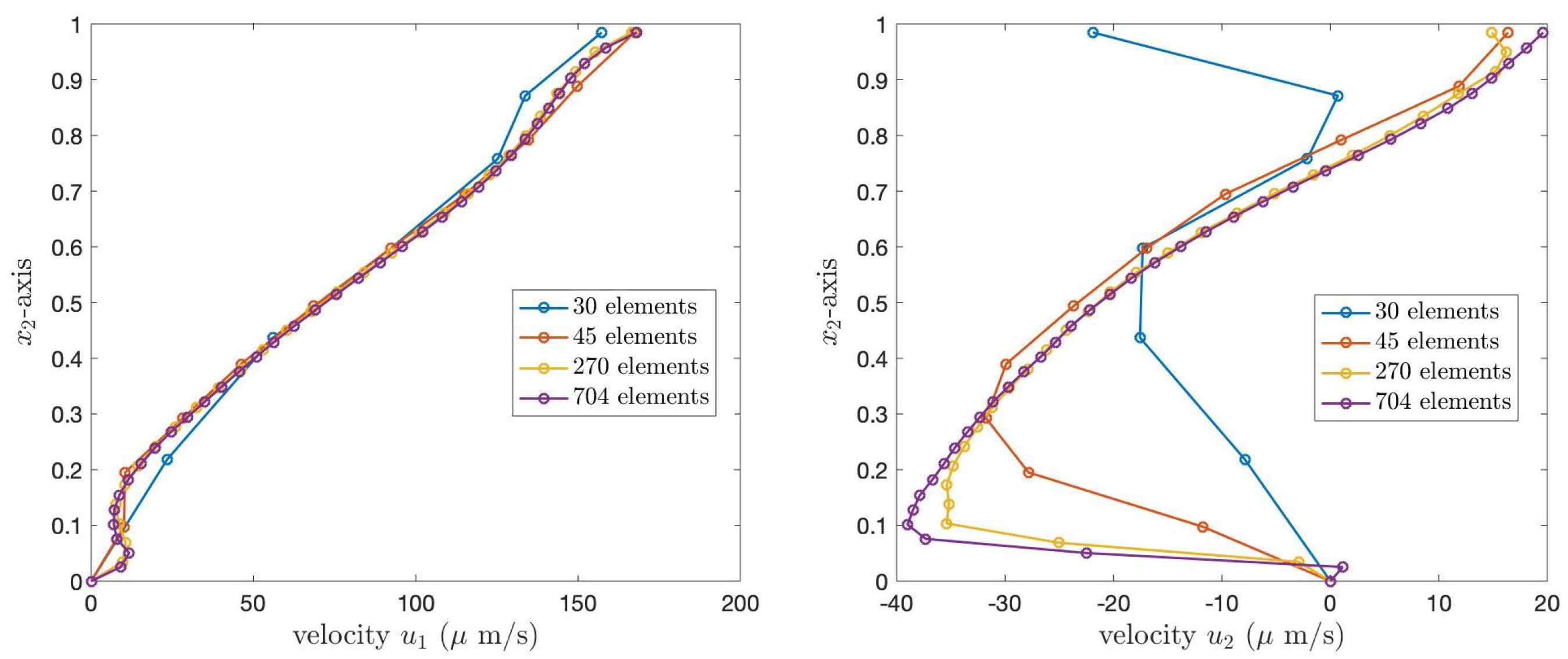
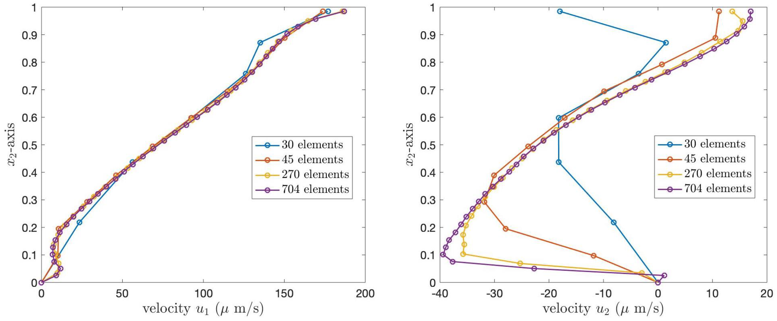
To validate the code, we choose to present the velocity profile of the PCL fluid when $\theta ={80}^{\circ }$. Since, in our work, we consider two cases of the boundary conditions, we provide our numerical results for the two cases. Figure 8 and Figure 9 illustrate the PCL velocities for Case 1 and Case 2 boundary conditions, respectively. In both figures, the left graph shows the velocity, $u_1$, and the right graph presents $u_2$. The blue, orange, yellow, and purple lines represent the velocity of the PCL fluid obtained from the grid refinements containing 30, 45, 270, and 704 elements, respectively. In both figures, the numerical solutions obtained from the coarser grids converge to the numerical solutions obtained from the finest grid.

Table 2. The $l_2$-norm errors of the PCL velocity obtained from the different mesh refinements at the angle $\theta ={80}^{\circ }$.

Number of Elements	${\mathit{l}}_2$-Norm Errors
	Case 1		Case 2
	${\mathit{u}}_{\mathbf{1}}$	${\mathit{u}}_{\mathbf{2}}$	${\mathit{u}}_{\mathbf{1}}$	${\mathit{u}}_{\mathbf{2}}$
30	17.8755	52.3543	18.1664	47.3204
45	8.8341	30.1146	15.3896	30.7428
270	8.8134	15.1360	9.7240	14.8701

presents the $l_2-$norm errors of the velocities $u_1$ and $u_2$ of the PCL fluid at the angle $\theta ={80}^{\circ }$, compared to the solutions obtained from the finest grid, 704 elements. The results show that the errors decrease as the number of elements increases, illustrating the convergence of the numerical solutions.

6. Numerical Results

The numerical solutions of the generalized Brinkman equation and the continuity equation, Equations (11) and (12), are presented in this section. The existence and uniqueness of the numerical solution using the mixed finite element method have been proven in [33]. We use the two-dimensional finite element method to determine the velocities of the PCL fluid propelled via moving cilia in the porous medium. We present the velocity of the PCL fluid when cilia make an angle of ${90}^{\circ }$ to ${40}^{\circ }$ to the horizontal plane. Two cases of the boundary conditions are considered. The values of the dynamic viscosity, fluid density, gravity, and the coefficients $c_i,i=1,2,3,4,$ are the same as in Section 5.

We use the triangular mesh with 270 elements and 579 points generated via Netgen [43], as shown in Figure 7. The numerical domain $\mathrm{\Omega }$ is divided into 10 subdomains. The first subdomain starts from the leftmost vertical line, at $\theta ={90}^{\circ }$, to the inclined line, at $\theta ={85}^{\circ }$. The second subdomain is next to the right of the first subdomain, starting from $\theta ={85}^{\circ }$ to $\theta ={80}^{\circ }$. Continuing the process until reaching $\theta ={40}^{\circ }$, we have 10 different subdomains. By using the mixed finite element method of Taylor–Hood type, we obtain the numerical results, which are illustrated in Figure 10. The first row of Figure 10 shows the velocities of the PCL fluid using the Case 1 boundary condition. 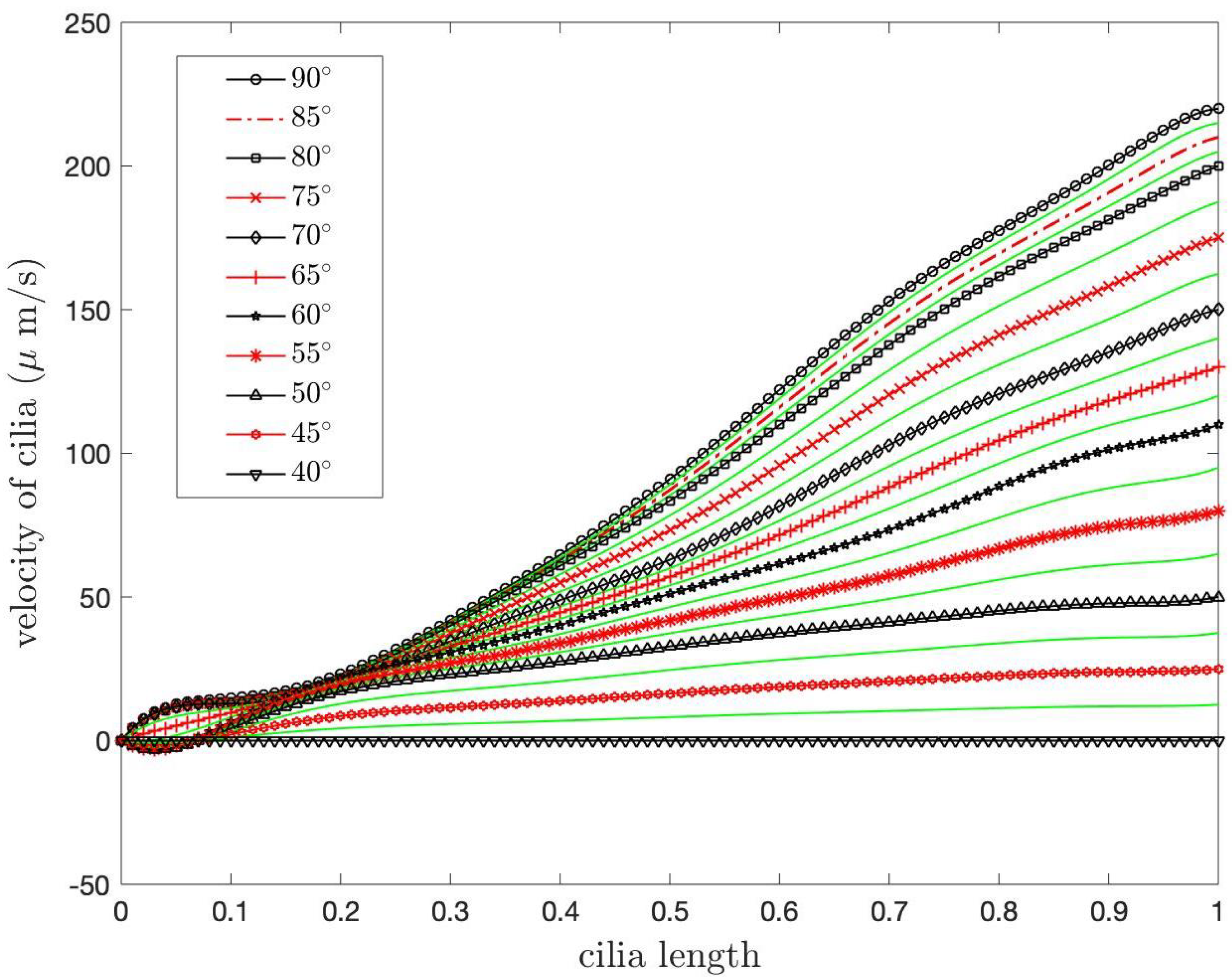The top left graph represents the velocity $u_1$ in the $x_1$ direction, while the top right graph presents the velocity $u_2$ in the $x_2$ direction. The velocity of the PCL fluid decreases when the angle decreases. This is affected by the velocity of the cilia; see Figure 6. The velocity $u_1$ is highest when $\theta ={90}^{\circ }$, and the velocity is zero at $\theta ={40}^{\circ }$ because the velocity of cilia is highest at $\theta ={90}^{\circ }$, and the cilia stop beating at $\theta ={40}^{\circ }$. For the velocity $v_2$, when the angle decreases, the velocity $u_2$ at the tips of cilia decreases from $110.74$ to $-36.64$ µm/s and then increases slightly until the velocity approaches zero at $\theta ={40}^{\circ }$. The velocity $u_2$ is negative because, for the forward bend direction of cilia, the vertical velocity changes from the positive to the negative direction. The second row of Figure 10 illustrates the velocities $u_1$ and $u_2$ of the PCL fluid under the Case 2 boundary condition for the angles ranging from $\theta ={90}^{\circ }$ to ${40}^{\circ }$. The bottom left graph presents the velocity, $u_1$, and the bottom right graph represents the velocity, $u_2$. In this case, we assume that the boundary condition at ${\mathrm{\Gamma }}_2$, at the tips of the cilia, is unknown. Similar to Case 1, the velocity $u_1$ of the PCL fluid reduces as the angles decrease, and the maximum velocity of the PCL fluid occurs at the tips of cilia. The difference in $u_1$ between Case 1 and Case 2 is that the velocity at the tips of cilia in Case 2 appears like a wave, moving up and down at the free interface. Similar to Case 1, the velocity $u_2$ is highest at the tips of cilia at $\theta ={90}^{\circ }$. As the angle decreases, the velocity $u_2$ at the tips of cilia reduces from $90.39$ to $-37.06$ µm/s before gradually increasing in the positive direction until it reaches zero at $\theta ={40}^{\circ }$. We also observe that the velocity $u_2$ at the tips of cilia in this case is smaller than the velocity $u_2$ in Case 1 for all angles.

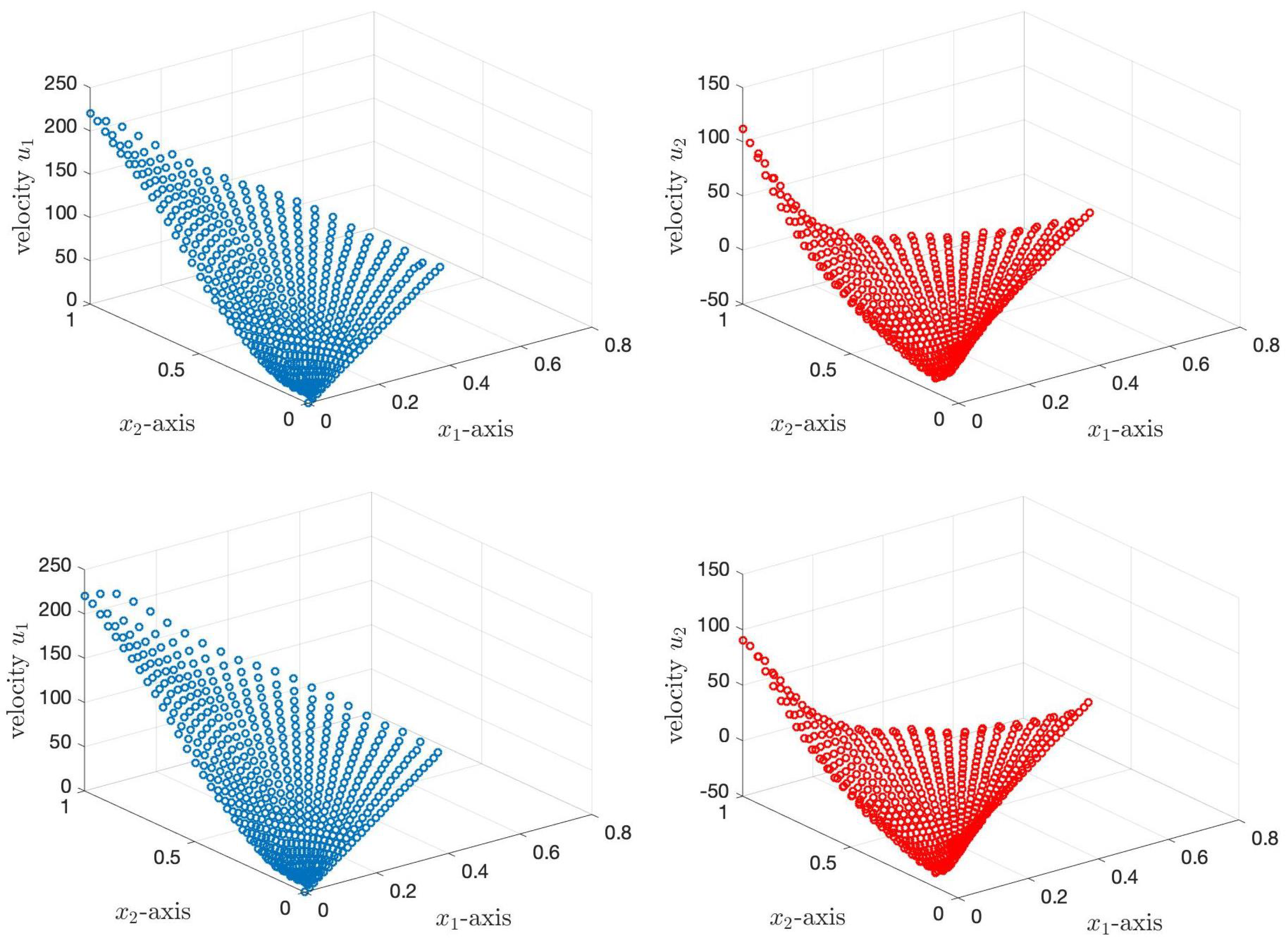
Next, we average the velocities $u_1$ and $u_2$ of the PCL fluid over the $x_1$-axis. The first row of Figure 11 shows the average velocities of the PCL fluid for the Case 1 boundary condition, while the second row illustrates the average velocities of the PCL fluid for the Case 2 boundary condition. The top left graph shows the average velocity of $u_1$, while the top right graph shows the average velocity of $u_2$. The average velocities of $u_1$ and $u_2$ are almost the same for both cases. For the velocity $u_2$, near the root of cilia, the velocity has a negative value and the velocity gradually increases to a positive value along the cilia until the tips of the cilia. The highest average velocities are at the tips of cilia for all cases. The mean velocities of $u_1$ for Case 1 and Case 2 are $46.55$ and $47.26$ µm/s, respectively. The mean velocities of $u_2$ for Case 1 and Case 2 are $-13.95$ and $-14.57$ µm/s, respectively. The mean velocities for both cases of $u_1$ are close to the velocity of the PCL fluid obtained from experimental data [45].

Researchers studied the movements of PCL and mucus in human tracheobronchial epithelial cell cultures using conventional and confocal microscopy of fluorescent microspheres. They found that the PCL fluid and mucus move at similar rates, $39.2\pm 4.7$ and $39.8\pm 4.2$ µm/s, respectively, which is close to our mean velocity, $u_1$, for both cases.

Figure 12 shows the speed of the PCL fluid of both cases of the boundary conditions. The left and right graphs illustrate the speed of the PCL fluid for Case 1 and Case 2, respectively. The shapes of the graphs for both cases are similar to the velocity $u_1$ except at the bottom of the representations. The difference comes from the effect of the negative value $u_2$ near the root of cilia. It shows that the velocity $u_1$ is more impactful to the PCL-fluid movement than $u_2$. The average speeds of the PCL fluid for Case 1 and Case 2 are $54.68$ µm/s and $55.45$ µm/s, respectively. The numerical results are compared with the numerical results provided in [13,14,25]. The authors determined the velocity of the PCL fluid due to the self-propelled cilia in one-dimensional, two-dimensional, and three-dimensional domains. In [13], the researchers used the finite element method to solve the nonlinear Stokes–Brinkman equations in a one-dimensional domain, and they discovered that the average speed of the PCL fluid was $54.98$ µm/s. In [14], the authors solved the nonlinear Brinkman equation in two dimensions using a mixed finite element method and Newton’s method to obtain the velocity of the PCL fluid. They found that the average speed for all angles, ${40}^{\circ }<\theta \le {90}^{\circ }$, was $52.52$ µm/s. In [25], the researchers determined the velocity of the PCL fluid caused by cilia beating using a mixed finite element method of Taylor–Hood type to solve the Stokes–Brinkman equations in a three-dimensional domain. The average speed over angles, ${40}^{\circ }<\theta \le {90}^{\circ }$, was found to be $52.52$ µm/s. Comparing the numbers with our results reveals that the maximum difference is $2.03$ µm/s or about $3.6\%$. These comparisons demonstrate that the average speed for both cases obtained in our simulations is close to the average speed of the PCL fluid reported in the literature.

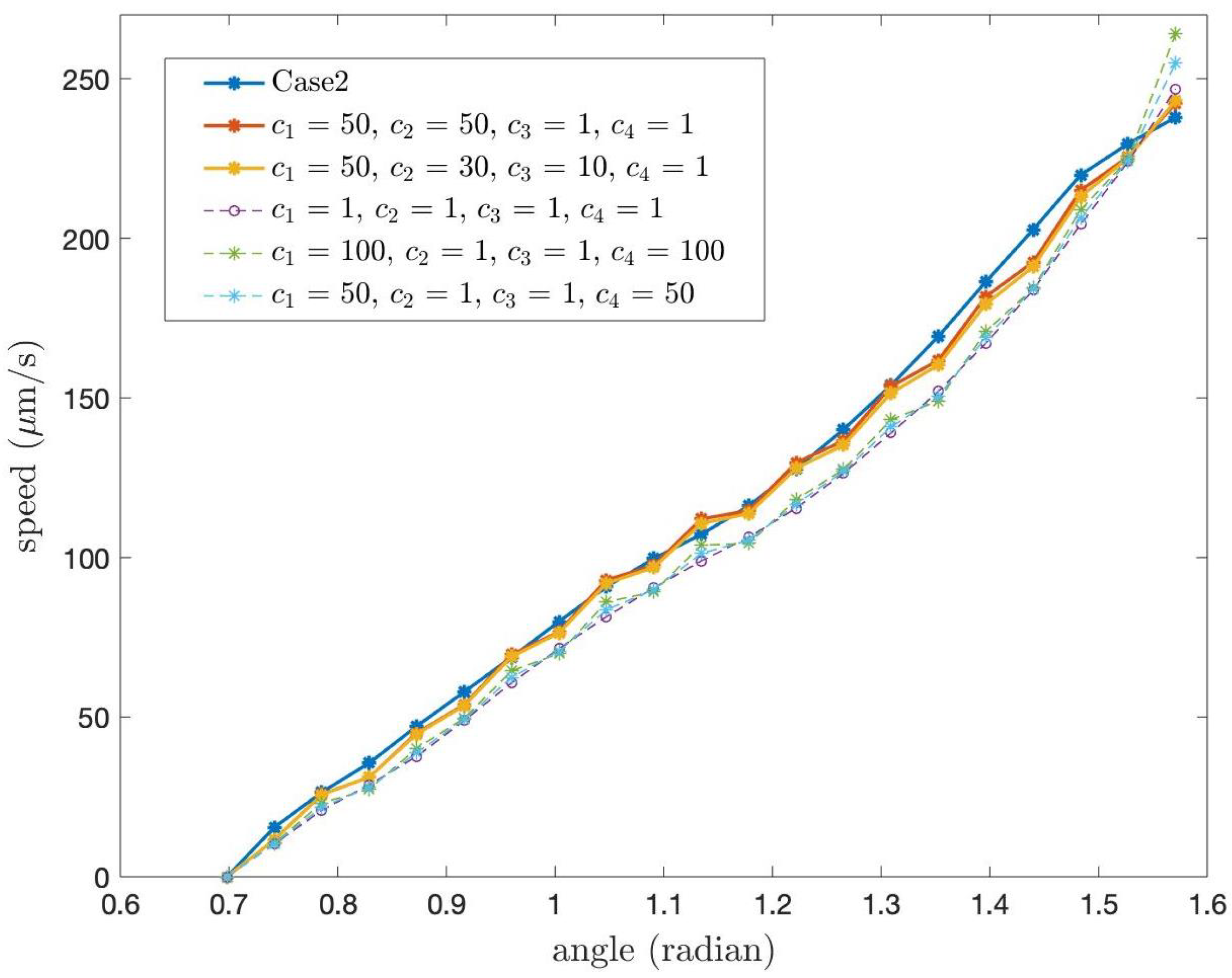
Next, we study the speed of the PCL fluid at the tips of cilia for different constants, $c_i,i=1,2,3,4,$ which are the coefficients in the boundary condition at ${\mathrm{\Gamma }}_2$ of Case 1. In the previous numerical results, we used $c_i=1$ for all i. For other values of $c_i,i=1,2,3,4,$ we present the speed of the PCL fluid at the tips of cilia in Figure 13 and Figure 14. Figure 13 shows the speed at the tips of cilia when $c_1=c_2=c_3=c_4=c,$ where $c=1,10,20,30,40,50$. From the graph, it can be observed that the different values of $c_i$ result in slight variations in speed. Figure 14 illustrates the speed of the PCL fluid at the tips of cilia when the values of $c_i,i=1,2,3,4$, are not equal. We also present the speed of the PCL fluid at the tips of cilia for Case 2 in order to compare the speed for Case 1 and Case 2 with different value of $c_i,i=1,2,3,4$. From the graph, we observe that the red and yellow lines are close to the line of Case 2. We also found that, despite different values of $c_i$, the shapes of all speed profiles in Figure 13 and Figure 14 are similar.

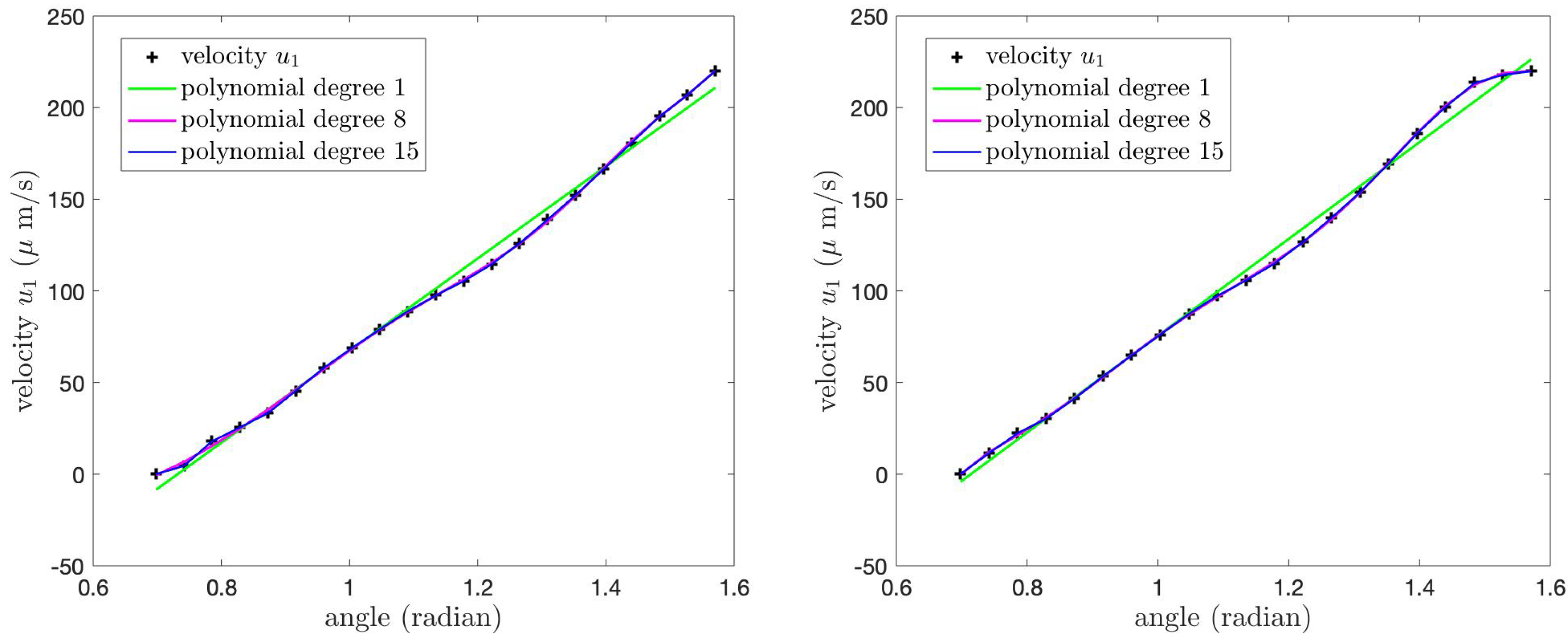
Because the velocity of the PCL fluid at the tips of cilia affects the velocity of mucus and the thickness of mucus can cause lung diseases, we focus on the velocity at the tips of cilia. We provide polynomial approximations of the velocities $u_1$ and $u_2$, as well as the speed of the PCL fluid at the tips of cilia for both cases of the boundary conditions illustrated in Figure 15, Figure 16 and Figure 17. We use $c_1=c_2=c_3=c_4=1$. Here, we provide the polynomial approximations of degrees 1, 8, and 15 for the velocities $u_1$ and the speed at the tips of cilia because the velocity $u_1$ and the speed profiles at the tips of cilia can be approximated by straight lines with an acceptable error, and sometimes it is convenient to use the first-degree polynomials for some problems. The polynomial approximations of degrees 8 and 15 are provided for $u_2$. In these figures, the horizontal axis represents the angle, measured in radians, ranging from ${40}^{\circ }$ to ${90}^{\circ }$. The green, magenta, and blue lines represent the polynomial approximations of degrees 1, 8, and 15, respectively. Figure 15 shows the velocity $u_1$ of the PCL fluid at the tips of the cilia and its polynomial approximations for Case 1 (left) and Case 2 (right) boundary conditions. We find that the velocity $u_1$ at the tips of the cilia in both cases increases as the angle $\theta$ increases from ${40}^{\circ }$ to ${90}^{\circ }$ and the maximum velocity occurs at the angle $\theta ={90}^{\circ }$.

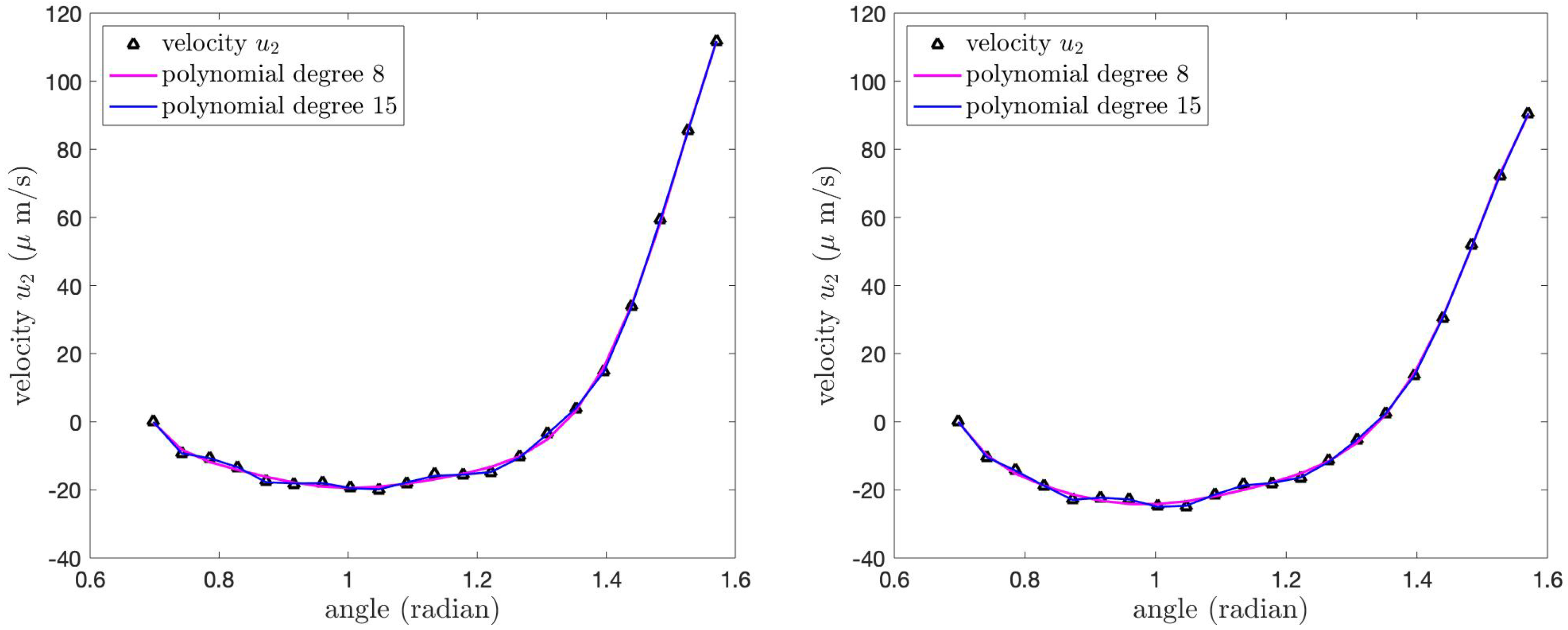
Figure 16 illustrates the velocity $u_2$ of the PCL fluid at the tips of the cilia and its polynomial approximations for both cases of the boundary conditions. The velocity $u_2$ for the Case 1 boundary condition (left) is greater than the velocity $u_2$ for the Case 2 boundary condition (right), especially at $\theta ={90}^{\circ }$. Although the shapes of the graphs in both cases have similar shapes, the values of the velocity $u_2$ are different. The velocity $u_2$ is the maximum at $\theta ={90}^{\circ }$, and then it decreases as the angle decreases until $\theta ={60}^{\circ }$. Then, the velocity increases until it reaches zero at $\theta ={40}^{\circ }$.

Figure 17 shows the speed of the PCL fluid at the tips of cilia and the first-, eighth-, and fifteenth-degree polynomial approximations for Case 1 (left) and Case 2 (right) boundary conditions. We see that the shapes of the speeds at the tips of cilia are similar to the shapes of the velocity $u_1$ for both cases; see Figure 15. This means the velocity $u_1$ affects the motion of the PCL fluid more than the velocity $u_2$.

From physical perspectives, the PCL fluid appears to move similarly to the motion of the cilia. That is, the velocity of the PCL fluid increases progressively from the base to the tips of cilia. As the cilia angle decreases, indicating greater bending, the fluid velocity at the tips also decreases, implying that propulsion efficiency is reduced during the motion. Since cilia are self-propelled organelles that move forward speedily and back gently, they perform their power stroke to move fluids, and then they gradually back to their starting position, which is slower than the forward stroke. This pattern of acceleration and deceleration repeats periodically due to the nature of cilia. As a result, the PCL fluid moves faster when the cilia are upright (effective stroke), slows down during the bending, and then accelerates again when the cilia are in the upright position, resulting in a pulsatile flow pattern similar to metachronal waves.

The polynomial functions and their coefficients are given in

Table 3. The first-degree polynomial function: $p\left(\theta \right)=a_1\theta +a_2$ estimates the speed and the velocities $u_1$ at the tips of cilia for both cases of the boundary conditions, where $\theta$ is the angle in radians.

Coefficients	Case 1
${10}^2\times$	Speed	Velocity $u_1$
$a_1$	2.61877889	2.51367073
$a_2$	−1.91617185	−1.83969272
Coefficients	Case 2
${10}^2\times$	Speed	Velocity $u_1$
$a_1$	2.68644586	2.64005346
$a_2$	−1.89878036	−1.88461055

,

Table 4. The eighth-degree polynomial function: $p\left(\theta \right)=a_1{\theta }^8+a_2{\theta }^7+a_3{\theta }^6+a_4{\theta }^5+a_5{\theta }^4+a_6{\theta }^3+a_7{\theta }^2+a_8\theta +a_9$ estimates the speed and the velocities $u_1$ and $u_2$ at the tips of cilia for both cases of the boundary conditions, where $\theta$ is the angle in radians.

Coefficients		Case 1
${10}^6\times$	Speed	$u_1$	$u_2$
$a_1$	−0.012734118271167	0.057378313095743	0.008776158423867
$a_2$	0.135670026652116	−0.500821282568611	−0.107483926304666
$a_3$	−0.617877401645130	1.885859004719336	0.527199931990443
$a_4$	1.572260187763733	−4.001363507459469	−1.393202912554586
$a_5$	−2.445640591057800	5.233621138954125	2.203387221815350
$a_6$	2.381652851245531	−4.323269305568677	−2.155213357695548
$a_7$	−1.418299927611897	2.204332823035274	1.280981336161525
$a_8$	0.472589132393864	−0.634706944987602	−0.424880299024707
$a_9$	−0.067549690623399	0.079037225239463	0.060416408378815
Coefficients		Case 2
${10}^6\times$	Speed	$u_1$	$u_2$
$a_1$	−0.010939237329981	0.015621983213058	0.008379732732943
$a_2$	0.124622237256656	−0.112413273633599	−0.100340169104345
$a_3$	−0.597329420016729	0.319219155174230	0.484478291821826
$a_4$	1.580853921698133	−0.425346939699839	−1.264833543315435
$a_5$	−2.535184997493686	0.184504901777252	1.980693486623330
$a_6$	2.529299675528232	0.190169061295289	−1.921683695840503
$a_7$	−1.536399388702010	−0.289319521303333	1.134790516797084
$a_8$	0.520744248609177	0.143704103345063	−0.374654504988026
$a_9$	−0.075587763208465	−0.026064000222104	0.053145691955595

and

Table 5. The fifteenth-degree polynomial function: $p\left(\theta \right)=a_1{\theta }^{15}+a_2{\theta }^{14}+a_3{\theta }^{13}+a_4{\theta }^{12}+a_5{\theta }^{11}+a_6{\theta }^{10}+a_7{\theta }^9+a_8{\theta }^8+a_9{\theta }^7+a_{10}{\theta }^6+a_{11}{\theta }^5+a_{12}{\theta }^4+a_{13}{\theta }^3+a_{14}{\theta }^2+a_{15}\theta +a_{16}$ estimates the speed and the velocities $u_1$ and $u_2$ at the tips of cilia for both cases of the boundary conditions, where $\theta$ is the angle in radians.

Coefficients		Case 1
${10}^{13}\times$	Speed	$u_1$	$u_2$
$a_1$	0.000148633026563	0.000238695384065	0.000026480736805
$a_2$	−0.002550402419714	−0.004115644913638	−0.000605547516345
$a_3$	0.020326208989479	0.032955135924412	0.006026245594933
$a_4$	−0.099800320623606	−0.162544503017583	−0.035447475762319
$a_5$	0.337572785098084	0.552225554160010	0.139568160750811
$a_6$	−0.833149607242801	−1.368720582565515	−0.392545818489031
$a_7$	1.549823716319571	2.556522729178357	0.818652144300971
$a_8$	−2.212460020243270	−3.663952619805488	−1.293279880109145
$a_9$	2.443567136385676	4.061961701798492	1.563966870703912
$a_{10}$	−2.087818866919695	−3.483132513082045	−1.450226545717761
$a_{11}$	1.368634146361897	2.291168271604290	1.024021239349936
$a_{12}$	−0.675937881127803	−1.135256083953165	−0.541256467049189
$a_{13}$	0.243443136497010	0.410133386662197	0.207457763075095
$a_{14}$	−0.060357509441902	−0.101981304210337	−0.054469949954978
$a_{15}$	0.009211069453411	0.015605585109138	0.008764590893595
$a_{16}$	−0.000652224105843	−0.001107808266398	−0.000651810809226
Coefficients		Case 2
${10}^{13}\times$	Speed	$u_1$	$u_2$
$a_1$	0.000161729298700	0.000296703434881	0.000331043699638
$a_2$	−0.002663547237013	−0.004991231500699	−0.005772032762279
$a_3$	0.020339099732280	0.038977801794141	0.046722649194728
$a_4$	−0.095508127683471	−0.187426343684253	−0.232891653324938
$a_5$	0.308374706749317	0.620563020263077	0.799355226552687
$a_6$	−0.725042308960541	−1.498477240355366	−2.000992476154122
$a_7$	1.282121070283650	2.725929439835820	3.773595128776208
$a_8$	−1.736005918233114	−3.803798599185942	−5.458846767793530
$a_9$	1.814220029861536	4.104776739782694	6.106696174312163
$a_{10}$	−1.462981962075676	−3.425342914369116	−5.282486588179633
$a_{11}$	0.902659332059763	2.192185648577189	3.504347199487991
$a_{12}$	−0.418360013949618	−1.056619726773176	−1.750716165522668
$a_{13}$	0.140946840215663	0.371266424291172	0.637552371208520
$a_{14}$	−0.032574870988444	−0.089776224139980	−0.159766249185166
$a_{15}$	0.004616166473962	0.013358553374243	0.024633814653303
$a_{16}$	−0.000302225539089	−0.000922051337170	−0.001761674965389

. Table 3 illustrates the coefficients of the first-degree polynomial function. Table 4 and Table 5 show the coefficients of the eighth- and fifteenth-degree polynomial functions, respectively.

The $l_2$-norm errors of the polynomial approximations of the velocity $u_1$ are presented in

Table 6. $l_2$-norm errors of the polynomial approximations of the velocity $u_1$ for both cases of the boundary conditions.

Order of Polynomial	${\mathit{l}}_2$- Norm Errors of Case 1	${\mathit{l}}_2$- Norm Errors of Case 2
1	23.37590758	22.60410473
8	4.49732994	2.54515053
15	0.77551149	0.67652906

. Table 6 shows the errors of the first-, eighth-, and fifteenth-degree polynomials. When the degree of the polynomial increases, the error decreases. Although the 15th-degree polynomials provide the best fitting, we also present the lower-order approximations because, in some cases, one may need only a rough estimate.

The $l_2$-norm errors of the polynomials approximating $u_2$ are shown in

Table 7. $l_2$-norm errors of the polynomial approximations for both cases of the boundary conditions.

Order of Polynomial	${\mathit{l}}_2$- Norm Errors of Case 1	${\mathit{l}}_2$- Norm Errors of Case 2
8	4.22075638	3.90055486
15	0.84113482	1.05561499

. In Table 7, we present the errors of the eighth- and fifteenth-order polynomials. The 15th-order approximation has better error than the 8th-order polynomial, but we also present both of them here because the smaller degree of the polynomial may be useful for some rough study cases.

The $l_2$-norm errors of the polynomial approximations of the speed at the tips of cilia are provided in

Table 8. $l_2$-norm errors of the polynomial approximations of the speed at the tips of cilia for both cases of the boundary conditions.

Order of Polynomial	${\mathit{l}}_2$- Norm Errors of Case 1	${\mathit{l}}_2$- Norm Errors of Case 2
1	45.26933528	28.93285837
8	2.54321963	2.58729001
15	0.49442221	0.47532558

. The errors are small for the 15th-order approximation.

7. Conclusions

In this research, we have studied the fluid flow problem in the periciliary layer (PCL) of the respiratory system in human lungs. We focused on the fluid moved via self-propelled bundles of cilia, rather than via pressure gradient. Here, we considered the PCL as a porous medium, which consists of the PCL fluid and cilia. To determine the velocity of the PCL fluid in the porous medium, we used the generalized Brinkman equation on a macroscopic scale with varied porosity for one fixed numerical domain. The numerical domain is designed to be the shape of a fan blade, imitating the actual beating pattern of cilia. The shape of the domain used in this study is closer to the pattern of the motion of cilia than the rectangular domain used in the previous literature. For the rectangular domain, authors have considered only one angle, $\theta$, for one fixed numerical domain. So, the porosity in their works was only a constant. In this work, our domain was designed to be aligned with the rotational movement of cilia, with which the cilia rotate around their roots. Therefore, the porosity used in the fan-blade domain is varied, depending on the angle, $\theta$, that the cilia make with the horizontal plane. We employ the mixed finite element method of the Taylor–Hood type to discretize the mathematical model and find the numerical solutions in the two-dimensional domain. We consider the forward movement of cilia making the angle ${90}^{\circ }$ to ${40}^{\circ }$ with the horizontal plane. We provide the velocities $u_1,u_2$ and the speed at the tips of cilia because it affects the velocity of mucus and then mucus thickness, which can cause diseases in the respiratory system in human lungs. At the tips of cilia, the velocity $u_1$ for the Case 1 boundary condition is lower than the velocity $u_1$ for Case 2, about $8.86\%$. Therefore, the boundary condition of Case 1 at the tips of cilia, which is expressed in the explicit form and is easy to apply to problems, may be used as a boundary condition at the free interface not only in this problem but also in other problems that are similar to this one, if the percentage difference is in an acceptable range of the problems. We provide the velocities and the speed of the PCL fluid for different values of $c_i$ so that they can be a guideline for those interested in applying this research to their works. We also present the first-, eighth-, and fifteenth-order polynomial functions for the velocities $u_1$ and $u_2$, as well as the speed at the tips of the cilia, in order to apply them to future work and other similar efforts.

If the velocity of the solid phases in our governing equations is neglected, the system of equations can be applied to fluid-flow problems with immobile solids, such as natural rice fields or trees, glass rods, engine filters, filter pads, and underground oil. In future work, we will predict the PCL fluid velocity with the full forward stroke of cilia from the angles ${130}^{\circ }$ to ${40}^{\circ }$ [39], as well as extend the problem to two domains: a porous medium and an adjacent free-fluid region. We will use the result from this study as a lower boundary condition to find the mucus velocity.

References

1. Lyons, R.A.; Saridogan, E.; Djahanbakhch, O. The reproductive significance of human Fallopian tube cilia. Hum. Reprod. Update 2006, 12, 363–372. [Google Scholar] [CrossRef] [PubMed]
2. Pechenik, J.A. Biology of the Invertebrates, 4th ed.; Tufs University: Medford, MA, USA; McGraw-Hill: New York, NY, USA, 1976; p. 305. [Google Scholar]
3. Bustamante-Marin, X.M.; Ostrowski, L.E. Cilia and mucociliary clearance. Cold Spring Harb. Perspect. Biol. 2017, 9, a028241. [Google Scholar] [CrossRef] [PubMed]
4. Walsh, D.; Bevan, J.; Harrison, F. How Does Airway Surface Liquid Composition Vary in Different Pulmonary Diseases, and How Can We Use This Knowledge to Model Microbial Infections? Microorganisms 2024, 12, 732. [Google Scholar] [CrossRef] [PubMed]
5. Zhu, P.; Chen, D.; Xu, Y. Simulation study on the mass transport in PCL based on the ciliated dynamic system of the respiratory tract. J. Phys. Conf. Ser. 2019, 1300, 012068. [Google Scholar] [CrossRef]
6. Poopra, S.; Wuttanachamsri, K. On the asymptotic boundary condition at the free-fluid/porous-medium interface in periciliary layer due to the ciliary movement. Math. Probl. Eng. 2022, 2022, 1390486. [Google Scholar] [CrossRef]
7. Vanaki, S.M.; Holmes, D.; Jayathilake, P.G.; Brown, R. Three-dimensional numerical analysis of periciliary liquid layer: Ciliary abnormalities in respiratory diseases. Appl. Sci. 2019, 9, 4033. [Google Scholar] [CrossRef]
8. Jayathilake, P.G.; Tan, Z.; Le, D.V.; Lee, H.P.; Khoo, B.C. Three-dimensional numerical simulations of human pulmonary cilia in the periciliary liquid layer by the immersed boundary method. Comput. Fluids 2012, 67, 130–137. [Google Scholar] [CrossRef]
9. Sedaghat, M.H.; Sadrizadeh, S.; Abouali, O. Three-dimensional simulation of mucociliary clearance under the ciliary abnormalities. J. Nonnewton. Fluid Mech. 2023, 316, 105029. [Google Scholar] [CrossRef]
10. Milosevic, M.; Stojanovic, D.B.; Simic, V.; Grkovic, M.; Bjelovic, M.; Uskokovic, P.S.; Kojic, M. Preparation and modeling of three-layered PCL/PLGA/PCL fibrous scaffolds for prolonged drug release. Sci. Rep. 2020, 10, 11126. [Google Scholar] [CrossRef]
11. Oangwatcharaparkan, N.; Wuttanachamsri, K. The flow in periciliary layer in human lungs with Navier-Stokes-Brinkman equations. Tamkang J. Math. 2023, 54, 107–120. [Google Scholar]
12. Poopra, S.; Wuttanachamsri, K. The velocity of PCL fluid in human lungs with beaver and Joseph boundary condition by using asymptotic expansion method. Mathematics 2019, 7, 567. [Google Scholar] [CrossRef]
13. Phaenchat, S. On the One-Dimensional Nonlinear Stokes-Brinkman Equations for Modeling Flow in PCL. Master’s Thesis, King Mongkut’t Institute of Technology, Ladkrabang, Thailand, 2019. [Google Scholar]
14. Phaenchat, S.; Wuttanachamsri, K. Two-dimensional nonlinear Brinkman and steady-state Navier–Stokes equations for fluid flow in PCL. Partial Differ. Equ. Appl. Math. 2024, 12, 100961. [Google Scholar] [CrossRef]
15. Conti, M.; Giorgini, A. Well-posedness for the Brinkman–Cahn–Hilliard system with unmatched viscosities. J. Differ. Equ. 2020, 268, 6350–6384. [Google Scholar] [CrossRef]
16. Titi, E.S.; Trabelsi, S. Global well-posedness of a three-dimensional Brinkman-Forchheimer-Bénard convection model in porous media. arXiv 2022, arXiv:2204.03531. [Google Scholar]
17. Coclite, G.M.; Mishra, S.; Risebro, N.H.; Weber, F. Analysis and numerical approximation of Brinkman regularization of two-phase flows in porous media. Comput. Geosci. 2014, 18, 637–659. [Google Scholar] [CrossRef]
18. Hansbo, P.; Juntunen, M. Weakly imposed Dirichlet boundary conditions for the Brinkman model of porous media flow. Appl. Numer. Math. 2009, 59, 1274–1289. [Google Scholar] [CrossRef]
19. Jia, J.; Lee, Y.J.; Feng, Y.; Wang, Z.; Zhao, Z. Hybridized weak Galerkin finite element methods for Brinkman equations. Electron. Res. Arch. 2021, 29, 2489–2516. [Google Scholar] [CrossRef]
20. Ouadefli, L.E.; Akkad, A.E.; Moutea, O.E.; Moustabchir, H.; Elkhalfi, A.; Scutaru, M.L.; Muntean, R. Numerical simulation for Brinkman system with varied permeability tensor. Mathematics 2022, 10, 3242. [Google Scholar] [CrossRef]
21. Chamsri, K. Formulation of a well-posed Stokes-Brinkman problem with a permeability tensor. J. Math. 2015, 1, 1–7. [Google Scholar]
22. Rinehart, A.; Lācis, U.; Bagheri, S. The Brinkman viscosity for porous media exposed to a free flow. arXiv 2021, arXiv:2106.01879. [Google Scholar]
23. Wuttanachamsri, K. Free interfaces at the tips of the cilia in the one-dimensional periciliary layer. Mathematics 2020, 8, 1961. [Google Scholar] [CrossRef]
24. Basirat, F.; Sharma, P.; Fagerlund, F.; Niemi, A. Experimental and modeling investigation of CO2 flow and transport in a coupled domain of porous media and free flow. Int. J. Greenh. Gas Control 2015, 42, 461–470. [Google Scholar] [CrossRef]
25. Wuttanachamsri, K.; Schreyer, L. Effects of cilia movement on fluid velocity: II numerical solutions over a fixed domain. Transp. Porous Media 2020, 134, 471–489. [Google Scholar] [CrossRef]
26. Nishad, C.S.; Chandra, A.; Karmakar, T.; Raja Sekhar, G.P. A non-primitive boundary element technique for modeling flow through non-deformable porous medium using Brinkman equation. Meccanica 2018, 53, 2333–2352. [Google Scholar] [CrossRef]
27. Abo-Elkhair, R.E.; Mekheimer, K.S.; Moawad, A.M.A. Cilia walls influence on peristaltically induced motion of magneto-fluid through a porous medium at moderate Reynolds number: Numerical study. J. Egypt. Math. Soc. 2017, 25, 238–251. [Google Scholar] [CrossRef]
28. Cortez, R.; Cummins, B.; Leiderman, K.; Varela, D. Computation of three-dimensional Brinkman flows using regularized methods. J. Comput. Phys. 2010, 229, 7609–7624. [Google Scholar] [CrossRef]
29. Deo, S.; Ansari, I.A.; Srivastava, B.G. On the general stream function solution of Brinkman equation in the cylindrical polar coordinates. Adv. Theo. Appl. Mech. 2016, 9, 21–30. [Google Scholar] [CrossRef]
30. Kanafiah, S.F.H.M.; Kasim, A.R.M.; Zokri, S.M.; Shafie, S. Numerical solutions of convective transport on Brinkman-viscoelastic fluid over a bluff body saturated in porous region. Case Stud. Therm. Eng. 2021, 28, 101341. [Google Scholar] [CrossRef]
31. Pranowo, P.; Wijayanta, A.T. Numerical solution of Darcy-Brinkman-Forchheimer equation for forced-convective fluid flow through porous medium using DMLPG method. AIP Conf. Proc. 2020, 2217, 030171. [Google Scholar]
32. Sleigh, M.A. Ciliary adaptations for the propulsion of mucus. Biorheology 1990, 27, 527–532. [Google Scholar] [CrossRef]
33. Kumankat, N.; Wuttanachamsri, K. Well-posedness of generalized Stokes-Brinkman equations modeling moving solid phases. Electron. Res. Arch. 2023, 31, 1641–1661. [Google Scholar] [CrossRef]
34. Cushman, J.H.; Bennethum, L.S.; Hu, B.X. A primer on upscaling tools for porous media. Adv. Water Resour. 2002, 25, 1043–1067. [Google Scholar] [CrossRef]
35. Bennethum, L.S. Multiscale, Hybrid Mixture Theory for Swelling Systems with Interfaces; Lecture Note; University of Colorado: Denver, CO, USA, 2007. [Google Scholar]
36. Bennethum, L.S.; Cushman, J.H. Multiscale, hybrid mixture theory for swelling systems—I: Balance laws. Int. J. Eng. Sci. 1996, 34, 125–145. [Google Scholar] [CrossRef]
37. Wuttanachamsri, K.; Schreyer, L. Effects of cilia movement on fluid velocity: I model of fluid flow due to a moving solid in a porous media framework. Transp. Porous Media. 2021, 136, 699–714. [Google Scholar] [CrossRef]
38. Weinstein, T.; Bennethum, L.S. On the derivation of the transport equation for swelling porous materials with finite deformation. Int. J. Eng. Sci. 2006, 44, 1408–1422. [Google Scholar] [CrossRef]
39. Sears, P.R.; Thompson, K.; Knowles, M.R.; Davis, C.W. Human airway ciliary dynamics. Am. J. Physiol. Lung Cell. Mol. Physiol. 2012, 304, 170–183. [Google Scholar] [CrossRef] [PubMed]
40. Brenner, S.C.; Scott, L.R. The Mathematical Theory of Finite Element Methods; Springer: New York, NY, USA, 2008. [Google Scholar]
41. Chamsri, K.; Bennethum, L.S. Permeability of fluid flow through a periodic array of cylinders. Appl. Math. Model. 2015, 39, 244–254. [Google Scholar] [CrossRef]
42. ICRP. Measurement: Human Respiratory Tract Model for Radiological Protection; ICRP Publication 66. Ann. ICRP; ICRB: Ottawa, ON, Canada, 1994; Volume 24, pp. 1–3. [Google Scholar]
43. Scho¨berl, J. NETGEN An advancing front 2D/3D-mesh generator based on abstract rules. Comput. Visual. Sci. 1997, 1, 41–52. [Google Scholar]
44. Woodfield, J.; Alvarez, M.; Gòmez-Vargas, B.; Ruiz-Baier, R. Stability and finite element approximation of phase change models for natural convection in porous media. J. Comput. Appl. Math. 2019, 360, 117–137. [Google Scholar] [CrossRef]
45. Matsui, H.; Randell, S.H.; Peretti, S.W.; Davis, C.W.; Boucher, R.C. Coordinated clearance of periciliary liquid and mucus from airway surfaces. J. Clin. Investig. 1998, 102, 1125–1131. [Google Scholar] [CrossRef]
Figure 1. Left: human respiratory system. Right: a portion of the trachea in the human respiratory tract.
Mathematics 13 01703 g001
Figure 2. Rectangular domain.
Mathematics 13 01703 g002
Figure 3. Left: the fan-blade shape of the porous domain on the x 1 x 2 plane when cilia make angles with the horizontal plane. Right: the illustration of the length ξ along cilia at the point ( x 1 a , x 2 a ) and the variable ξ max .
Mathematics 13 01703 g003
Figure 4. The boundary of our domain.
Mathematics 13 01703 g004
Figure 5. The geometric cells of the periodic array of five cylinders in three dimensions.
Mathematics 13 01703 g005
Figure 6. Speed of cilia along the cilia length.
Mathematics 13 01703 g006
Figure 7. Generated mesh for the numerical domain.
Mathematics 13 01703 g007
Figure 8. The velocities of the PCL fluid obtained from four different mesh refinements at the angle θ = 80 for the Case 1 boundary condition. The left graph is the velocity u 1 , while the right graph is the velocity u 2 .
Mathematics 13 01703 g008
Figure 9. The velocities of the PCL fluid obtained from four different mesh refinements at the angle θ = 80 for the Case 2 boundary condition. The left graph is the velocity u 1 , while the right graph is the velocity u 2 .
Mathematics 13 01703 g009
Figure 10. The velocities u 1 (left) and u 2 (right) of the PCL fluid for all angles. The first row shows the velocities for the Case 1 boundary condition while the second row shows the velocities for the Case 2 boundary condition.
Mathematics 13 01703 g010
Figure 11. The average velocities u 1 and u 2 of the PCL fluid. The top left shows the average velocity u 1 of Case 1, while the top right presents the average velocity u 2 of Case 1. The bottom left shows the average velocity u 1 of Case 2, while the bottom right presents the average velocity u 2 of Case 2.
Mathematics 13 01703 g011
Figure 12. The left figure shows the speed of the PCL fluid for the Case 1 boundary condition, and the right figure presents the speed for the Case 2 boundary condition.
Mathematics 13 01703 g012
Figure 13. The speed of the PCL fluid at the tips of cilia for Case 1 boundary condition when c 1 = c 2 = c 3 = c 4 = c , c = 1 , 10 , 20 , , 50 .
Mathematics 13 01703 g013
Figure 14. The speed of the PCL fluid at the tips of cilia with different values of c i for i = 1 , 2 , 3 , 4 .
Mathematics 13 01703 g014
Figure 15. The velocity u 1 of the PCL fluid at the tips of the cilia for Case 1 boundary condition (left) and for Case 2 boundary condition (right).
Mathematics 13 01703 g015
Figure 16. The velocity u 2 of the PCL fluid at the tips of cilia for Case 1 boundary condition (left) and for Case 2 boundary condition (right).
Mathematics 13 01703 g016
Figure 17. The speed of the PCL fluid at the tips of cilia for Case 1 boundary condition (left) and for Case 2 boundary condition (right).
Mathematics 13 01703 g017