A Hybrid Vector Autoregressive Model for Accurate Macroeconomic Forecasting: An Application to the U.S. Economy

Abstract

Forecasting macroeconomic variables is essential to macroeconomics, financial economics, and monetary policy analysis. Due to the high dimensionality of the macroeconomic dataset, it is challenging to forecast efficiently and accurately. Thus, this study provides a comprehensive analysis of predicting macroeconomic variables by comparing various vector autoregressive models followed by different estimation techniques. To address this, this paper proposes a novel hybrid model based on a smoothly clipped absolute deviation estimation method and a vector autoregression model that combats the curse of dimensionality and simultaneously produces reliable forecasts. The proposed hybrid model is applied to the U.S. quarterly macroeconomic data from the first quarter of 1959 to the fourth quarter of 2023, yielding multi-step-ahead forecasts (one-, three-, and six-step ahead). The multi-step-ahead out-of-sample forecast results (root mean square error and mean absolute error) for the considered data suggest that the proposed hybrid model yields a highly accurate and efficient gain. Additionally, it is demonstrated that the proposed models outperform the baseline models. Finally, the authors believe the proposed hybrid model may be expanded to other countries to assess its efficacy and accuracy.

1. Introduction

An economy’s overall economic growth can be determined by its growth rate. Economic growth is a key indicator of a country’s development, often reflected in an increase in the Gross Domestic Product (GDP). Economic growth is highly desirable since it generally indicates that society as a whole is becoming wealthier. Several factors, including technological advancements, rising consumer demand for products and services, and an expanding labor force, can contribute to economic growth. The prospects of stable macroeconomic factors improve any country’s financial stability and economic growth. They include an increase in the demand for goods and services. Favorable macroeconomic environments facilitate a greater flow of capital into an economy, thereby propelling the industry. Some of the key macroeconomic indicators include GDP growth, the Consumer Price Index (CPI), Money Supply (MS), Unemployment Rate, Government Debt, Inflation Rate, Current Account, Government Deficit, and Stock Market Volatility. These characteristics are essential for any economy worldwide. If these indicators significantly increase, the economy is more likely to expand [1,2,3,4].

GDP is essential, as it gives data on the size and prosperity of the economy. Real GDP growth is often used as a measure of the economy’s overall well-being. Typically, growing real GDP is viewed as a positive indicator of the country’s economic improvement. Another critical factor is the spread of the MS, as inflation will occur if it grows faster than the economy can afford to deliver goods and services. However, production may decline, and unemployment would increase if the Money Supply did not grow quickly enough. In general, as the GDP growth rate shows higher economic productivity, the value of a currency in circulation increases [5,6,7,8].

This allows each money unit to be later exchanged for more expensive goods and services, as identified, which is why the CPI should measure inflation [9,10]. The CPI is also used to determine a person’s eligibility for benefits, such as Social Security, and to guide wage adjustments that reflect changes in the cost of living. The growth and forecasting of these macroeconomic variables are of great interest to economists and policymakers because they are crucial to an economy. The forecasting of these variables is comparable to the forecasting of the economy’s overall growth rate. In conclusion, three primary macroeconomic variables—GDP, CPI, and MS—are crucial to a nation’s development [11,12,13,14].

The motivation for proposing novel hybrid steps stems from two primary reasons. Increasing the number of variables initially leads to high multicollinearity between the covariates. Secondly, we face the problem of degrees of freedom. In time series analysis, one of the top-rated forecasting models, the VAR model, often engages in these issues. To avoid dual problems and to make them more efficient, the VAR model was augmented by a penalty term, referring to sparse VAR models. With time, few penalties were used, including LASSO and elastic net. As a case study, we apply the proposed model to quarterly macroeconomic data from the U.S., demonstrating its practical utility in identifying key drivers of economic performance. Furthermore, no previous study has combined the smoothly clipped absolute deviation (SCAD) regularization method with VAR to forecast macroeconomic or financial variables. Thus, we propose a novel hybrid of the SCAD and VAR (sparse VAR) models, aiming to mitigate the problem of biased sparse VAR models, such as the Least Absolute Shrinkage and Selection Operator (LASSO), Ridge Regression (RG), and Elastic Net (EN), in forecasting. The new hybrid model is highly beneficial when a large set of covariates is available. In addition, unlike existing sparse VAR models, the novel hybrid model selectively identifies relevant variables that are nearly unbiased while encouraging the coefficients of irrelevant variables to approach zero.

The remainder of the paper is structured as follows. Section 2 provides an overview of the previous work, and Section 4 discusses the techniques and models utilized to create the innovative hybrid model. Section 5 applies the proposed hybrid model to the U.S. quarterly microeconomic data. Finally, Section 6 discusses the conclusions, limits, and future research prospects.

2. Literature Review

Numerous forecasting methods can be used depending on the data structure and pattern [15,16,17,18,19]. They include regularized least squares methods, such as the LASSO, RG, and EN, as discussed in [20]. Similarly, to analyze macroeconomic variables, many articles have employed machine learning (ML) techniques and factors to forecast these variables [21,22,23,24,25,26]. For example, Giannone et al. [27] evaluated the predictive power of sparse modeling using a Bayesian prediction framework that included LASSO, ridge, and elastic net to macroeconomic data. A LASSO-VAR model was used by [28] to predict the Japanese macroeconomic series. The predictability of ML tools based on regression trees, such as random forest, was highlighted by [29,30]. Using U.S. macroeconomic data, Ng and Bai [30] examined the effectiveness of boosting techniques for forecasting inflation, industrial production, interest rates, unemployment, and employment rates. Some researchers have applied neural networks to macroeconomic forecasting, including [31] for the U.S. inflation series, Shintani [32] for the Japanese macroeconomic series, and [33] for the U.S. unemployment series. Lunde and Torkar [34] used a principal component analysis (PCA) to reduce the number of variables after using more than 120 predictors. The PCA does not provide a standard output interpretation despite using several information sources in their configuration. However, the literature that investigates forecasting tools for macroeconomic variables primarily focuses on the applications of various VAR specifications as seen in the studies of [35,36,37]. The appropriate Bayesian shrinkage procedures help improve forecasting as discussed in [38]. The yield curve, which provides insight into future economic activity, is widely recognized as one potential economic indicator that can be used to forecast GDP. This concept has been discussed in various studies [39,40]. It was determined that the yield curve slope could predict cumulative changes in real GDP up to four years into the future by [41]. Bernard and Gerlach [42] studied yield curves in eight countries. They found that, despite significant differences across the countries, the yield slope indicates the prospective frequency of recessions. Several studies, including [43,44,45], utilized a list of macroeconomic indicators to provide projections regarding the GDP of the United States.

In ref. [46], Sims first proposed VAR models to understand economic linkages in 1980, and they are now frequently used for the structural analysis and real-time forecasting of numerous temporally observable variables. The traditional VAR suffers from a dimensionality problem. The Bayesian VAR technique, proposed by [47], addresses this issue by handling the dimensionality problem through the use of priors to reduce the number of variables. The factor-augmented VAR model, recommended by [48], is another approach for dimensionality. The predicted variable and the calculated predictor factor estimate in this model serve as arguments in a typical VAR model. In recent studies, LASSO was used to shrink the parameter space of a VAR model as discussed in the works of [49,50]. Aydin and Cavdar [51] compared the ANN and VAR models and concluded that the ANN outperforms the VAR model.

Marcellino [52] compared the forecast performance of the 58 models for a large dataset of 500 macroeconomic variables for the European Monetary Union (EMU). Their results indicate that a single non-linear model outperforms other models. Secondly, the results also suggest that the performance of both pooled forecasts and non-linear models increases if only unstable series are considered. In a single time window, Yan et al. [53] compared their logistic, support vector machine (SVM), decision tree, and artificial neural network (ANN) models and concluded that SVM and ANN perform better in this context. Fokin and Polbin [54] examined Russia’s significant macroeconomic variables, including GDP, fixed asset investment, household consumption, exports, imports, the real ruble exchange rate, and oil prices, applying the LASSO VAR model. It is also evident that many models have fairly reasonable predictive ability when pseudo-real-time values are compared with actual values from the Ministry of Economic Development’s forecast. However, Li et al. [55] compared LASSO-based and dynamic factor models for forecasting macroeconomic variables. They concluded that all LASSO-based models outperform dynamic factor models in out-of-sample forecast evaluations. The work [56] applies LASSO-VAR to very short-term wind power forecasting. On the other hand, Araujo and Gaglianone [57] compared 53 different forecasting methods, including machine learning methods with application to Brazil’s inflation data. Their results show that machine learning techniques outperform traditional forecasting methods. The work of [58] analyzed recent advances in supervised machine learning and high-dimensional data models for forecasting. They discussed linear and non-linear settings and concluded that machine learning approaches can provide more accurate forecasts for financial time series. In the same way, Goulet Coulombe et al. [59] compared machine learning forecasting methods, including linear and non-linear models. According to their results, non-linear models are uncertain in forecasting macroeconomic variables compared to regularization, cross-validation, and alternative loss functions.

This study addresses this gap by proposing a novel SCAD-penalized VAR model to enhance both variable selection and forecasting accuracy for macroeconomic indicators. To our knowledge, this is one of the first empirical applications of SCAD-penalized VAR models to forecast high-dimensional macroeconomic indicators, thereby highlighting their novelty and contribution to the existing literature. The use of SCAD in conjunction with VAR models offers a methodologically robust approach that combines sparsity with lower bias, which is particularly important when dealing with noisy and multicollinear macroeconomic data. In contrast, SCAD achieves a balance between variable selection and coefficient estimation, allowing for more stable and interpretable models in macroeconomic settings. Moreover, most current studies focus on convex penalties, which can overshrink significant coefficients, limiting the model’s interpretability and generalization performance. SCAD, known for its oracle properties and unbiased variable selection, offers a promising alternative that has not been thoroughly explored in macroeconomic forecasting. While LASSO and Elastic Net remain popular, their inherent bias in variable selection can impair forecast accuracy, especially in high-dimensional contexts. Despite these advancements, there is still limited work on integrating non-convex regularization techniques, such as the SCAD penalty, within the VAR framework.

3. Methodology

By merging time series data from multiple nearby sites, the VAR model enables the simultaneous provision of an accurate forecast for the underlying economic series. On the other hand, forecasting with VAR models may be impossible for high-dimensional data because the non-sparse coefficient matrix grows quadratically with the number of series incorporated into the model. To circumvent this issue, Ref. [50] proposed a blend of LASSO and VAR frameworks, which was further explored by [56].

It is a fact that traditional methodologies are ineffective in cases involving high-dimensional data. In contrast, capturing the dynamic nature of the economic system is essential for robust/better policy, which is often ignored in the case of high-dimensional data. Therefore, this study combines two different methodologies—the penalized regression model and VAR—to address the limitations of the separate models. LASSO is biased in its variable selection [60]. Thus, we utilize SCAD in conjunction with VAR to select relevant variables in an unbiased manner, aiming for more robust and efficient forecasts.

3.1. Formulation of the Forecasting Models

By capturing the linear interdependencies in the multiple time series, the VAR model enables us to analyze the joint dynamic behavior of a set of variables. The future value of each series is determined by its lags; the lags of other series are considered in the model [61]. Let ${\mathrm{M}}_t$ be the time series representing the average values of an outcome variable at time t, such as CPI, MS, and GDP. An outcome variable is supposed to be a linear combination of its past values and lagged variables, plus a random error term [62]. Mathematically, it can be illustrated as

$$M_t=\delta +{\kappa }_1{M}_{t-1}+{\kappa }_2{M}_{t-2}+\dots +{\kappa }_s{M}_{t-s}+{ϵ}_t+{\aleph }_1{ϵ}_{t-1}+{\aleph }_2{ϵ}_{t-2}+\dots +{\aleph }_n{ϵ}_{t-n}$$

(1)

In Equation (1), ${\kappa }_j$ ($j=1,2,\dots ,s$) and ${\aleph }_l$ ($l=1,2,\dots ,n$) are all the unknown parameters to be estimated from the available data; j and l represent the order of autoregressive (AR) and moving average (MA), and ${ϵ}_t$ is contemporaneous white noise (or residuals) with constant variance ${\delta }_{ϵ}^2$ and zero mean. To identify the suitable AR process and MA component for a specific time series, numerous criteria are referenced in the literature [63,64,65]. In our scenario, we utilize the auto.arima function from the R-package, version 2023.09.1 forecast, for model selection.

Let $\{M_t\}=\{{(m_{1,t},m_{2,t},\dots ,m_{p,t})}^{\prime }\}$ represent a vector time series with p dimensions. By incorporating all these variables into the model, we obtain the vector of response variables, and the future value of p variables is determined by the lags of all variables, a process known as vector autoregression in the literature. The mathematical expression is as follows:

$$M_t=\omega +\sum _{j=1}^s{K}^{\left(j\right)}{M}_{t-j}+{ϵ}_t$$

(2)

where $\omega$ indicates a vector of constant terms, $K^{\left(j\right)}$ represents the matrix of coefficients associated with the lags, and the ${ϵ}_t\sim (0,{\Sigma }_{ϵ})$ signifies a white noise error.

To express the VAR(s) model compactly, let $M=[M_{s+1},M_{s+2},\dots ,M_T]\in {\mathbb{R}}^{p\times t}$ denote the response matrix, where $t=T-s$. For each time point $t=s+1,\dots ,T$, define the stacked lag vector:

$$W_t=\left[\begin{array}{c}{M}_{t-1}\\ M_{t-2}\\ ⋮\\ M_{t-s}\end{array}\right]\in {\mathbb{R}}^{ps\times 1}$$

Then, define the matrix of lagged covariates as $W=[W_{s+1},W_{s+2},\dots ,W_T]\in {\mathbb{R}}^{ps\times t}$. Let $K=[K^{\left(1\right)}{K}^{\left(2\right)}\dots K^{\left(s\right)}]\in {\mathbb{R}}^{p\times ps}$ be the coefficient matrix, and $E=[{ϵ}_{s+1},\dots ,{ϵ}_T]\in {\mathbb{R}}^{p\times t}$ the matrix of residuals.

The VAR(s) model can then be written compactly as

$$M=\omega 1^{\prime }+KW+E,$$

(3)

where $\omega \in {\mathbb{R}}^{p\times 1}$ is the intercept vector, and $1^{\prime }\in {\mathbb{R}}^{1\times t}$ is a row vector of ones.

3.2. Sparse Structure of the VAR Model

This section presents a variety of sparse structures, including LASSO, elastic net, and SCAD, for the VAR model as influenced by [66] that captures the underlying dynamics of the system.

Let ${\parallel .\parallel }_r$ indicate both the matrix and vector $L_r$ norms. A loss function of the sparse-VAR estimator can be expressed as

$${\displaystyle \frac{1}{2}}{\parallel M-KW\parallel }_2^2+\vartheta {\parallel K\parallel }_r$$

(4)

As in Equation (4), the penalty function is represented by the second term in the preceding equation ${\vartheta \parallel K\parallel }_r$, which takes on different forms for various methods. The shrinking amount is adjusted by a tuning parameter denoted by the symbol $\vartheta$. The tuning parameter has a range from 0 to ∞.

Ridge Regression: If we replace the penalty with ${\vartheta \parallel K\parallel }_r=\vartheta {\parallel K\parallel }^2$, it induces another estimator that refers to ridge regression. The coefficient estimates of a ridge regression model are close to zero but not strictly equal to zero. In other words, variable selection is not performed using this method.

LASSO: We can obtain the sparse LASSO-VAR model by replacing the penalty in Equation (1) as follows: ${\vartheta \parallel K\parallel }_r=\vartheta {\parallel K\parallel }_1$, where the tuning parameter $\vartheta$ is typically determined through a cross-validation procedure [67]. By using the $L_1$ norm or LASSO penalty, many regression coefficients are forced to be exactly zero, and only the important predictors are kept. The LASSO estimator is biased in selecting important variables [68].

Elastic Net: Ref. [69] integrated two well-known penalties, namely $L_1$ and $L_2$, and put them in Equation (1) as ${\vartheta \parallel K\parallel }_r={\vartheta \parallel K\parallel }_1+\vartheta {\parallel K\parallel }_2^2$, resulting in an EN-VAR model. It retains the same representation sparsity as LASSO but produces a grouping effect.

Smoothly Clipped Absolute Deviation: The continuously differentiable penalty function is defined as follows:

$${\vartheta \parallel K\parallel }_r=r\{I(K\le r)+{\displaystyle \frac{{(\zeta r-K)}_{+}}{(\zeta -1)r}}I(K\le r)\}$$

(5)

for some $\zeta >2$, $K>0$ and $r>0$ is the SCAD penalty [70] where ${\vartheta \parallel K\parallel }_r=0$ and $\zeta \approx 3.7$ as recommended by [71]. The sparse SCAD-VAR model can be obtained by substituting the above-mentioned SCAD penalty in Equation (1).

3.3. SCAD-VAR Hybrid

This research proposes an innovative hybrid forecasting model that is extremely useful in situations with a large number of covariates. In contrast to the sparse VAR, the new hybrid model selects the relevant variables unbiasedly while setting the coefficients of irrelevant variables to zero. As a result, forecasting accuracy is substantially improved, and the desired results can be achieved with greater likelihood.

3.4. Statistical Loss Functions

To assess the predictability of ML algorithms against the ARIMA model, we compute the dual loss functions, namely the root mean square error (RMSE) and the mean absolute error (MAE) [72,73,74]. The model with the lowest RMSE and MAE is considered superior. Mathematically, the MAE and RMSE are illustrated as

$$MAE=\mathrm{mean}\left(\right|M_t-{\widehat{M}}_t\left|\right)$$

(6)

$$RMSE=\sqrt{\mathrm{mean}{(M_t-{\widehat{M}}_t)}^2},$$

(7)

where $M_t$ and ${\widehat{M}}_t$ indicate the observed and predicted GDP, CPI, and MS values.

In conclusion, all implementations are completed using R, a statistical computing language and environment. The packages used in the code are essential for various aspects of data analysis and model construction. The ‘sparsevar’ package facilitates the estimation of sparse vector autoregressive models, which is particularly beneficial for high-dimensional time series data. The ‘MLmetrics’ and ‘Metrics’ packages are utilized for model evaluation, offering a range of performance metrics to measure the predictive accuracy of the models. The ‘glmnet’ package is employed for fitting regularized regression models, such as LASSO and Ridge, which are helpful for feature selection and prediction in high-dimensional datasets. Additionally, the ‘forecast’ and ‘ncvreg’ packages are utilized for time series forecasting and regularization of linear regression models, respectively, thereby enhancing the robustness of the analysis. All computations are performed on an Intel Core i5-6200U CPU with a clock speed of 2.80 GHz.

4. Case Study Forecasting Results

The dataset used in this analysis includes quarterly time series data spanning from the first quarter of 1959 to the fourth quarter of 2023, collected from the Federal Reserve’s website (https://fred.stlouisfed.org, accessed on 2 May 2024). The main variables in the dataset are the Consumer Price Index (CPI), Gross Domestic Product (GDP), and M2 Money Supply (MS), which each serve as a response variable in individual models. These are selected to study macroeconomic trends and their interrelatedness over time. CPI is a crucial inflation measure, GDP captures economic production, and MS gives indications of liquidity and monetary policy. The dataset is sufficiently rich to enable a comprehensive analysis of these economic variables and their correlations with a range of explanatory variables. The time frame encompasses both phases of economic expansion and recession, making the dataset sufficiently rich to analyze the dynamics of these critical economic variables. Lastly, the external sector encompasses foreign investment, exchange rates, and trade balances, which indicate the position of the U.S. in the international economic system and its level of exposure to global markets. With this comprehensive list of variables, the study aims to create a complete picture of the U.S. macroeconomic landscape, thereby facilitating more reliable forecasting of key indicators such as GDP, CPI, and MS.

When modeling and predicting financial time series data, a crucial assumption is that the data must be stationary. A stationary process is characterized by having constant mean, variance, and autocorrelation structure over time. If the original series is non-stationary, it needs to be transformed into a stationary form. In various studies, several methods are employed to attain stationarity, including the application of the natural logarithm and differencing the data, or utilizing the Box-Cox transformation [75,76].

Table 1. Summary statistics and ADF test results for GDP, CPI, and MS (original, log, differenced, and log-differenced).

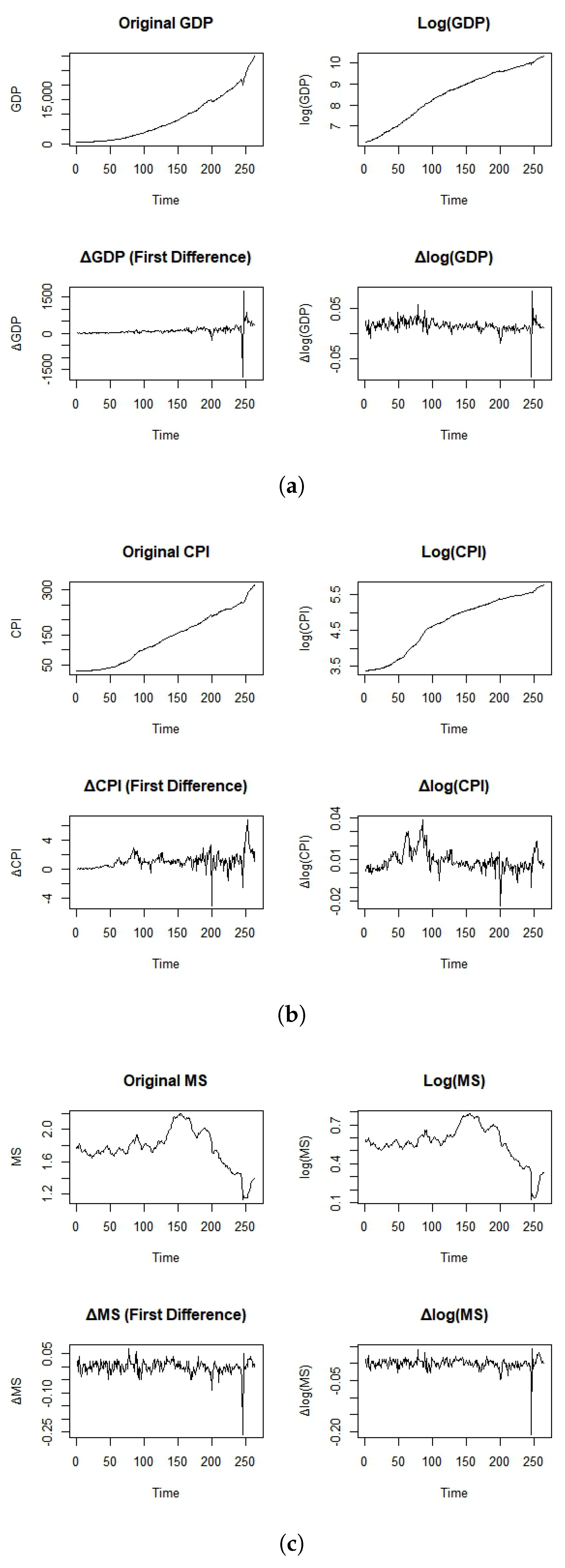
Series	Mean	Median	Variance	CV	Min	Max	Skewness	Kurtosis	ADF Stat (p-Val)
GDP	8769.9	6760.7	9.86 × 107	0.113	243.1	27,000.0	0.70	2.36	−1.78 (0.71)
log (GDP)	8.76	8.82	0.501	0.08	5.49	10.21	−0.28	2.17	−2.36 (0.40)
$\Delta$GDP	177.5	141.3	1.05 × 105	1.83	−642.5	1011.8	0.89	4.51	−3.91 (0.01)
$\Delta$log (GDP)	0.019	0.018	0.0002	0.74	−0.067	0.089	−0.02	2.83	−3.66 (0.03)
CPI	110.5	109.9	1535.6	0.35	23.5	303.3	0.93	2.66	−1.94 (0.62)
log (CPI)	4.57	4.70	0.396	0.14	3.16	5.71	−0.22	2.13	−2.81 (0.22)
$\Delta$CPI	1.48	1.40	3.46	1.26	−2.15	6.73	0.31	3.39	−3.25 (0.08)
$\Delta$log (CPI)	0.0129	0.0126	0.0003	1.36	−0.029	0.034	−0.10	2.57	−3.01 (0.12)
MS	3134.3	2063.8	1.22 × 107	1.12	139.9	9870.0	0.64	2.06	−1.55 (0.79)
log(MS)	7.63	7.63	0.540	0.096	4.94	9.20	−0.10	1.79	−2.49 (0.33)
$\Delta$MS	98.4	83.0	6.57 × 104	2.6	−1366.0	964.3	−0.51	4.47	−4.73 (0.00)
$\Delta$log (MS)	0.013	0.013	0.0002	1.09	−0.067	0.067	−0.13	2.60	−4.58 (0.00)

provides an analysis that includes descriptive statistics and unit root test findings for quarterly macroeconomic indicators in the U.S.—Gross Domestic Product (GDP), Consumer Price Index (CPI), and Money Supply (MS)—over a specified time frame, utilizing original, log-transformed, and first-order differenced data. In their original form, all three variables—GDP, CPI, and MS—demonstrate high average values and variances, signifying considerable magnitudes and significant variability. The coefficients of variation (CVs) are relatively low for GDP (0.113) and CPI (0.35), while they are notably high for MS (1.12), indicating that the Money Supply is relatively more unstable when compared to its average. Each of the three series shows positive skewness, indicating longer tails to the right, and their kurtosis values are marginally above 2, suggesting a slight leptokurtic tendency. The Augmented Dickey–Fuller (ADF) test results for the original series are not statistically significant (p-values > 0.5), indicating that the unadjusted series are non-stationary. The log-transformed series helps stabilize the variance. Log(GDP), log(CPI), and log(MS) exhibit lower variances and coefficients of variation (CVs), making them more suitable for modeling purposes. There is a reduction in skewness across all log-transformed series, and the kurtosis approaches that of a normal distribution (approximately 3), enhancing symmetry. Nonetheless, the ADF tests still reflect non-stationarity after the log transformation, with p-values remaining above conventional significance levels. Upon applying first-order differencing, both the original and log-transformed series exhibit significant reductions in variance and coefficient of variation (CV), indicating stabilization in both levels and dispersion. The differenced series—$\Delta$GDP, $\Delta$CPI, and $\Delta$MS—now exhibit considerably higher CVs, which is common for changes or growth rates. $\Delta$GDP and $\Delta$MS exhibit strong positive skewness and excess kurtosis, indicating that they are characterized by frequent minor changes accompanied by occasional substantial shifts. Importantly, the ADF test results for the differenced series are significant at the 1% or 5% levels, with most p-values falling below 0.05. This affirms that differencing effectively induces stationarity, which is essential for time series modeling methods such as ARIMA and VAR. In addition to numerical analysis, the visual analysis of these quarterly macroeconomic indicators, including GDP, CPI, and MS, is presented in Figure 1 for both original and log-transformed data, as well as first-order differenced and log-transformed first-order differenced data.

To sum up, after both presentation tables and graphs, the raw and log-transformed series for GDP, CPI, and MS are non-stationary as anticipated for macroeconomic aggregates. However, after implementing first-order differencing, the series exhibits stationarity, rendering them suitable for additional econometric modeling. The descriptive statistics further suggest that differencing not only achieves stationarity but also reduces skewness and kurtosis, thereby enhancing the normality and analytical feasibility of the series. Therefore, after addressing the concerns regarding non-stationarity and normality, we can proceed to model and predict quarterly forecasts for 1–3 and 6 steps ahead of key macroeconomic indicators in the U.S.—such as GDP, CPI, and MS—utilizing conventional time series models.

In this study, we denote each proposed VAR model as ${\mathrm{VAR}}_P$ for simplicity. Specifically, ${\mathrm{VAR}}_S$ refers to the VAR model with a SCAD penalty, ${\mathrm{VAR}}_L$ denotes the VAR model with a LASSO penalty, and ${\mathrm{VAR}}_E$ indicates the VAR model with an Elastic Net penalty. In contrast, the benchmark model ARIMA is represented as ${\mathrm{ARIMA}}_B$. For modeling and forecasting purposes, the dataset is separated into two halves to achieve the out-of-sample forecast error. To estimate the various models for GDP, CPI, and MS time series, we use data from 1959Q1 to 2010Q4 and from 2011Q1 to 2023Q4 to evaluate the 1–3 and 6-step-ahead forecasting accuracy of the models.

Table 2. Performance measures outcomes: RMSE and MAE for all models across varying forecast windows (1, 3, and 6 quarters ahead forecast).

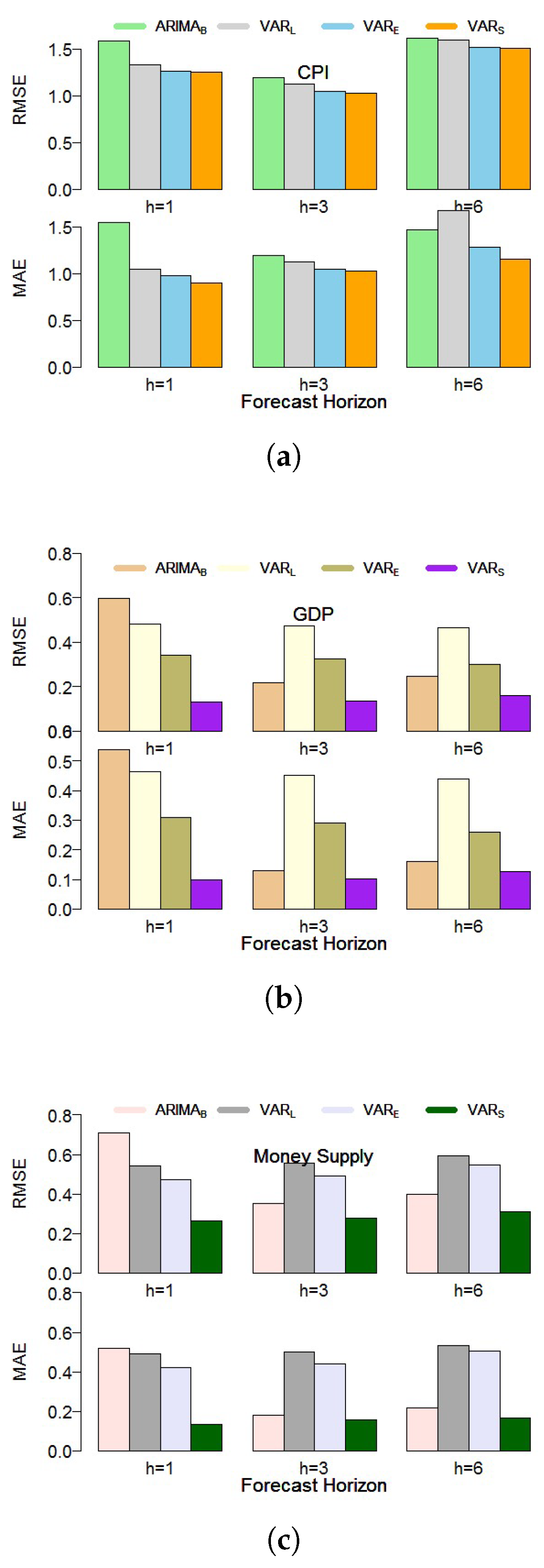
Variable		GDP		CPI		MS
Forecast Horizons	Methods	RMSE	MAE	RMSE	MAE	RMSE	MAE
$h=1$	${\mathrm{ARIMA}}_B$	0.596	0.538	1.589	1.547	0.711	0.518
	${\mathrm{VAR}}_L$	0.482	0.463	1.335	1.05	0.54	0.489
	${\mathrm{VAR}}_E$	0.34	0.308	1.266	0.979	0.473	0.422
	${\mathrm{VAR}}_S$	0.132	0.1	1.253	0.902	0.262	0.135
$h=3$	${\mathrm{ARIMA}}_B$	0.219	0.129	1.426	1.19	0.35	0.181
	${\mathrm{VAR}}_L$	0.472	0.451	1.413	1.126	0.556	0.501
	${\mathrm{VAR}}_E$	0.327	0.291	1.335	1.044	0.493	0.44
	${\mathrm{VAR}}_S$	0.137	0.102	1.417	1.026	0.279	0.156
$h=6$	${\mathrm{ARIMA}}_B$	0.249	0.159	1.615	1.464	0.398	0.219
	${\mathrm{VAR}}_L$	0.467	0.439	1.6	1.672	0.594	0.531
	${\mathrm{VAR}}_E$	0.302	0.259	1.513	1.282	0.548	0.505
	${\mathrm{VAR}}_S$	0.159	0.128	1.509	1.159	0.311	0.165

displays the results of each model’s forecasting experiments for three target macroeconomic variables—GDP growth, MS, and CPI—at various forecast horizons (h = 1, 3, 6). The RMSE and MAE are used as statistical metrics to evaluate the accuracy of the predictive models. This implies that the smaller the values of RMSE and MAE, the closer the predicted values are to the actual data. In the case of GDP growth, the one-step-ahead forecasting performance of ${\mathrm{VAR}}_P$ models is more efficient than the benchmark ARIMA model. Across the underlying models, it can be deduced that the ${\mathrm{VAR}}_S$ model outperforms the rival approaches. For the MS and CPI series, we discover that the ${\mathrm{VAR}}_S$ model shows a more robust forecast than ${\mathrm{ARIMA}}_B$ and competing approaches. Expanding the forecast horizons, such as h = 3, the RMSE and MAE associated with ${\mathrm{ARIMA}}_B$ are smaller than those of the dual ${\mathrm{VAR}}_P$ models, including ${\mathrm{VAR}}_L$ and ${\mathrm{VAR}}_E$. At the same time, ${\mathrm{VAR}}_S$ remains dominant in terms of minimal forecast errors. Similarly, when looking at longer time horizons for forecasting, i.e., h = 6, the RMSE and MAE of ${\mathrm{ARIMA}}_B$ are often lower than the ${\mathrm{VAR}}_L$ and ${\mathrm{VAR}}_E$, even though ${\mathrm{VAR}}_S$ is still the best in forecasting.

Table 2 displays the evaluation of various forecasting models based on their performance regarding three economic indicators—GDP, CPI, and MS—across multiple forecast horizons ($h=1,3,6$). The models under consideration include ${\mathrm{ARIMA}}_B$, ${\mathrm{VAR}}_L$, ${\mathrm{VAR}}_E$, and ${\mathrm{VAR}}_S$, with accuracy assessed using root mean square error (RMSE) and mean absolute error (MAE). A lower value in these metrics signifies enhanced forecasting accuracy.

In GDP forecasting, the ${\mathrm{VAR}}_S$ model consistently achieves the lowest levels of RMSE and MAE across all forecast horizons, with RMSE declining from 0.132 at $h=1$ to 0.159 by $h=6$. This indicates that ${\mathrm{VAR}}_S$ offers the most precise predictions for GDP. The ${\mathrm{ARIMA}}_B$ model, on the other hand, displays relatively poor performance, especially at $h=1$ (RMSE = 0.596), suggesting its inadequacy for short-term GDP forecasts.

When it comes to CPI forecasts, the ${\mathrm{VAR}}_S$ model again shows superior performance at $h=1$, with the lowest RMSE (1.253) and MAE (0.902). Nevertheless, at $h=3$, its RMSE (1.417) is only marginally better than that of ${\mathrm{VAR}}_E$ (1.335). At $h=6$, both ${\mathrm{VAR}}_S$ and ${\mathrm{VAR}}_E$ maintain RMSE and MAE values that are lower than those of ${\mathrm{ARIMA}}_B$ and ${\mathrm{VAR}}_L$, confirming their better performance in CPI forecasting.

For MS forecasts, ${\mathrm{VAR}}_S$ once again outshines the other models throughout all scenarios, recording the lowest RMSE and MAE across forecast horizons. Notably, at $h=1$, its RMSE (0.262) and MAE (0.135) are considerably lower than the corresponding values for ${\mathrm{ARIMA}}_B$ (RMSE = 0.711, MAE = 0.518), underscoring its effectiveness in capturing short-term fluctuations in MS.

In summary, the findings indicate that the ${\mathrm{VAR}}_S$ model consistently delivers the most precise forecasts for all three economic variables across all forecast horizons. Conversely, ${\mathrm{ARIMA}}_B$ generally ranks lowest, particularly concerning GDP and MS. ${\mathrm{VAR}}_E$ also demonstrates commendable performance, especially for CPI and MS at longer time horizons. These results suggest that ${\mathrm{VAR}}_S$ is the most dependable option for economic forecasting in this context.

Once the performance of the proposed hybrid model is evaluated by the loss function (RMSE and MAE), now move ahead and look at a graphical assessment. Figure 2 displays a collection of bar graphs that depict the performance of several forecasting models in estimating three economic metrics: Consumer Price Index (CPI), Gross Domestic Product (GDP), and Money Supply. The performance indicators utilized are root mean square error (RMSE) and mean absolute error (MAE), both of which assess the accuracy of the models’ forecasts, with lower values representing better performance. Each row in the diagram pertains to a specific economic metric: (a) CPI, (b) GDP, and (c) Money Supply. Within each row, the graphs depict the RMSE (top) and MAE (bottom) scores for three distinct forecast intervals: 1 quarter (h = 1), 3 quarters (h = 3), and 6 quarters (h = 6) ahead. The forecasting models assessed include ${\mathrm{ARIMA}}_B$ and three variations of Vector Autoregression (VAR) models: ${\mathrm{VAR}}_L$, ${\mathrm{VAR}}_E$, and ${\mathrm{VAR}}_S$, each represented by unique colors. Overall, the models’ performance varies based on different time horizons and economic indicators. For CPI, the RMSE and MAE values appear quite comparable across models, although certain models perform slightly better at various intervals. Regarding GDP, the ${\mathrm{VAR}}_S$ model (purple) consistently exhibits lower RMSE and MAE values, indicating it surpasses the others. In the case of Money Supply, the ${\mathrm{VAR}}_S$ model once again demonstrates lower error rates in comparison to the other models. This diagram emphasizes the relative efficacy of various forecasting models in predicting macroeconomic variables over differing time frames.

5. Discussion

This study proposes a novel hybrid model that combines the VAR model with a SCAD penalty term (${\mathrm{VAR}}_S$) to enhance forecasting accuracy. The study evaluates the performance of the proposed hybrid model against existing methods, including ARIMA and other sparse VAR models (${\mathrm{VAR}}_L$ and ${\mathrm{VAR}}_E$). This approach aligns with previous works in the literature that commonly compare various forecasting techniques to identify the most accurate method [77,78]. Like many previous studies (as discussed in the literature), this research focuses on forecasting essential macroeconomic variables such as GDP growth, CPI, and MS. This aligns with the broader literature, which recognizes the importance of accurately predicting these variables for economic analysis and policymaking.

Differences from previous studies can first be described as the novelty of the hybrid model. The study presents an innovative hybrid model that joins the VAR framework with the SCAD penalty term (${\mathrm{VAR}}_S$), a combination that has not been explored previously in the literature. This represents a significant departure from traditional approaches and contributes to the advancement of forecasting methodologies.

Secondly, the difference from previous works in the literature is the evaluation metrics: While previous studies commonly use metrics like RMSE and MAE to assess forecasting accuracy, this study provides a detailed comparison of these metrics across different forecast horizons (1, 3, and 6 quarters ahead). This comprehensive evaluation adds depth to the analysis and offers a comprehensive understanding of the model’s performance over varying time frames.

The discrepancies observed in the performance of the proposed hybrid model compared to existing methods highlight the importance of methodological innovation in forecasting macroeconomic variables. The outstanding performance of the hybrid model, particularly in certain forecast horizons, suggests that incorporating unbiased variable selection methods like SCAD into traditional models can lead to more accurate predictions.

Policymakers can utilize this novel strategy to enhance their decision-making process since the ${\mathrm{VAR}}_P$ model consistently demonstrates superior performance compared to conventional techniques like ARIMA and sparse VAR models. By offering more precise forecasts of crucial macroeconomic indicators such as GDP growth, MS, and CPI, policymakers may develop policies with greater assurance, resulting in more efficient economic administration and resource allocation.

The expanded forecasting skills of the ${\mathrm{VAR}}_P$ (particularly ${\mathrm{VAR}}_S$) model have the potential to benefit various stakeholders, such as enterprises, investors, and financial institutions. The enhanced understanding of forthcoming economic patterns enables stakeholders to enhance their strategic decision-making, mitigate potential risks, and uncover avenues for expansion. Ultimately, this phenomenon adds to the establishment of a more stable and prospering economic environment.

However, this study employs only sparse VAR models in addition to the standard ARIMA model. It is a fact that the VAR model preserves only short-run information and loses long-run information due to the difference transformation. Future research may focus on the sparse vector error correction model, which addresses the shortcomings of the VAR model. Additionally, a modified version of SCAD, known as “elastic SCAD”, can be utilized in conjunction with VAR and VECM to achieve even more substantial improvements in forecasting accuracy. Monte Carlo simulation experiments can be used to evaluate the statistical aspects of the proposed models.

6. Concluding Remarks

Forecasting macroeconomic indicators is crucial for the fields of macroeconomics, financial economics, and the analysis of monetary policy. The complex nature of macroeconomic datasets presents a challenge to the efficient and accurate forecasting of economic trends. Therefore, this research offers an in-depth examination of predicting macroeconomic indicators by contrasting various vector autoregressive models and different estimation methods. This study proposes a hybrid forecasting approach that combines a vector autoregressive (VAR) framework with the smoothly clipped absolute deviation (SCAD) penalty, resulting in a novel sparse VAR variant known as ${\mathrm{VAR}}_S$. The objective of the model is to enhance the accuracy of macroeconomic forecasts in comparison to traditional and biased sparse VAR models. The proposed hybrid model was applied to the U.S. quarterly microeconomic data from the first quarter of 1959 to the fourth quarter of 2023, yielding multi-step-ahead forecasts (one-, three-, and six-step ahead). The multi-step-ahead out-of-sample forecast results (root mean square error and mean absolute error) for the considered data suggest that the proposed hybrid model yields a highly accurate and efficient gain. Empirical findings, focusing on GDP growth, the Money Supply (MS), and the Consumer Price Index (CPI), indicate that the ${\mathrm{VAR}}_S$ model consistently yields lower RMSE and MAE values, especially in one-step and multi-step forecasting scenarios (h = 3 and h = 6). Importantly, ${\mathrm{VAR}}_S$ surpasses both the ${\mathrm{ARIMA}}_B$ model and the dual sparse VAR benchmarks (${\mathrm{VAR}}_L$ and ${\mathrm{VAR}}_E$) across the majority of indicators and time horizons. These results provide compelling evidence of the effectiveness of merging unbiased variable selection techniques with established time series models in macroeconomic forecasting. This strategy improves predictive accuracy without introducing the risk of overfitting. Future investigations should consider applying this hybrid method to other economic situations and assess its stability during different structural shifts or periods of economic turbulence. In summary, the ${\mathrm{VAR}}_S$ model represents a significant advancement for decision-makers and analysts seeking more reliable forecasting tools.

References

- Dědeček, R.; Dudzich, V. Exploring the limitations of GDP per capita as an indicator of economic development: A cross-country perspective. Rev. Econ. Perspect. 2022, 22, 193–217. [Google Scholar] [CrossRef]
- Zhang, S.; Li, X.; Zhang, C.; Luo, J.; Cheng, C.; Ge, W. Measurement of factor mismatch in industrial enterprises with labor skills heterogeneity. J. Bus. Res. 2023, 158, 113643. [Google Scholar] [CrossRef]
- Ren, Y.; Zhang, J.; Wang, X. How does data factor utilization stimulate corporate total factor productivity: A discussion of the productivity paradox. Int. Rev. Econ. Financ. 2024, 96, 103681. [Google Scholar] [CrossRef]
- Ma, Q.; Zhang, Y.; Hu, F.; Zhou, H. Can the energy conservation and emission reduction demonstration city policy enhance urban domestic waste control? Evidence from 283 cities in China. Cities 2024, 154, 105323. [Google Scholar] [CrossRef]
- Nneamaka, N.T. Prospects of Oil Palm Wine and Raphia Palm Wine in South East, Nigeria. Prospects 2019, 9, 31–35. [Google Scholar]
- Xi, X.; Xi, B.; Miao, C.; Yu, R.; Xie, J.; Xiang, R.; Hu, F. Factors influencing technological innovation efficiency in the Chinese video game industry: Applying the meta-frontier approach. Technol. Forecast. Soc. Change 2022, 178, 121574. [Google Scholar] [CrossRef]
- Zhao, S.; Zhang, L.; An, H.; Peng, L.; Zhou, H.; Hu, F. Has China’s low-carbon strategy pushed forward the digital transformation of manufacturing enterprises? Evidence from the low-carbon city pilot policy. Environ. Impact Assess. Rev. 2023, 102, 107184. [Google Scholar] [CrossRef]
- Chen, Q.; Han, Y.; Huang, Y.; Jiang, G.J. Jump Risk Implicit in Options Market. J. Financ. Econom. 2025, 23, nbaf002. [Google Scholar] [CrossRef]
- Chaudhary, S.K.; Xiumin, L. Analysis of the determinants of inflation in Nepal. Am. J. Econ. 2018, 8, 209–212. [Google Scholar]
- Shi, J.; Liu, C.; Liu, J. Hypergraph-Based Model for Modeling Multi-Agent Q-Learning Dynamics in Public Goods Games. IEEE Trans. Netw. Sci. Eng. 2024, 11, 6169–6179. [Google Scholar] [CrossRef]
- Amaral, A.; Dyhoum, T.E.; Abdou, H.A.; Aljohani, H.M. Modeling for the relationship between monetary policy and GDP in the USA using statistical methods. Mathematics 2022, 10, 4137. [Google Scholar] [CrossRef]
- Zhang, X.; Yang, X.; He, Q. Multi-scale systemic risk and spillover networks of commodity markets in the bullish and bearish regimes. N. Am. J. Econ. Financ. 2022, 62, 101766. [Google Scholar] [CrossRef]
- Zhao, S.; Zhang, L.; Peng, L.; Zhou, H.; Hu, F. Enterprise pollution reduction through digital transformation? Evidence from Chinese manufacturing enterprises. Technol. Soc. 2024, 77, 102520. [Google Scholar] [CrossRef]
- Wei, M.; Xiong, Y.; Sun, B. Spatial effects of urban economic activities on airports’ passenger throughputs: A case study of thirteen cities and nine airports in the Beijing-Tianjin-Hebei region, China. J. Air Transp. Manag. 2025, 125, 102765. [Google Scholar] [CrossRef]
- Shah, Z.; Abbas, G.; Khan, F. Deep learning in financial time series forecasting. Expert Syst. Appl. 2022, 207, 117033. [Google Scholar] [CrossRef]
- Zhang, S.; Roller, S.; Goyal, N.; Artetxe, M.; Chen, M.; Chen, S.; Zettlemoyer, L. Opt: Open pre-trained transformer language models. arXiv 2022, arXiv:2205.01068. [Google Scholar]
- Chang, X.; Gao, H.; Li, W. Discontinuous Distribution of Test Statistics Around Significance Thresholds in Empirical Accounting Studies. J. Account. Res. 2025, 63, 165–206. [Google Scholar] [CrossRef]
- Dong, X.; Yu, M. Time-varying effects of macro shocks on cross-border capital flows in China’s bond market. Int. Rev. Econ. Financ. 2024, 96, 103720. [Google Scholar] [CrossRef]
- Li, L.; Xia, Y.; Ren, S.; Yang, X. Homogeneity Pursuit in the Functional-Coefficient Quantile Regression Model for Panel Data with Censored Data. Stud. Nonlinear Dyn. Econom. 2024. [Google Scholar] [CrossRef]
- Kotchoni, R.; Leroux, M.; Stevanovic, D. Macroeconomic forecast accuracy in a data-rich environment. J. Appl. Econom. 2019, 34, 1050–1072. [Google Scholar] [CrossRef]
- Castle, J.L.; Doornik, J.A.; Hendry, D.F. Improving models and forecasts after equilibrium-mean shifts. Int. J. Forecast. 2024, 40, 1085–1100. [Google Scholar] [CrossRef]
- Luciani, M. Large-Dimensional Dynamic Factor Models in Real-Time: A Survey. Technical Report 2511872, SSRN. 2014. Available online: https://ssrn.com/abstract=2511872 (accessed on 25 May 2024).
- Swanson, N.R.; Xiong, W. Big data analytics in economics: What have we learned so far, and where should we go from here? Can. J. Econ. 2018, 51, 695–746. [Google Scholar] [CrossRef]
- Diebold, F.X.; Shin, M. Machine learning for regularized survey forecast combination: Partially-egalitarian lasso and its derivatives. Int. J. Forecast. 2019, 35, 1679–1691. [Google Scholar] [CrossRef]
- Swanson, N.R.; Xiong, W.; Yang, X. Predicting interest rates using shrinkage methods, real-time diffusion indexes, and model combinations. J. Appl. Econom. 2020, 35, 587–613. [Google Scholar] [CrossRef]
- Muhammadullah, S.; Urooj, A.; Khan, F.; Alshahrani, M.N.; Alqawba, M.; Al-Marzouki, S. Comparison of Weighted Lag Adaptive LASSO with Autometrics for Covariate Selection and Forecasting Using Time-Series Data. Complexity 2022, 2022, 2649205. [Google Scholar] [CrossRef]
- Giannone, D.; Lenza, M.; Primiceri, G.E. Economic Predictions with Big Data: The Illusion of Sparsity; Technical Report 847; Federal Reserve Bank of New York: New York, NY, USA, 2018. [Google Scholar]
- Nakajima, Y.; Sueishi, N. Forecasting the Japanese macroeconomy using high-dimensional data. Jpn. Econ. Rev. 2022, 73, 299–324. [Google Scholar] [CrossRef]
- Medeiros, M.C.; Vasconcelos, G.F.; Veiga, A.; Zilberman, E. Supplementary material for forecasting inflation in a data-rich environment: The benefits of machine learning methods. J. Bus. Econ. Stat. 2021, 39, 98–119. [Google Scholar] [CrossRef]
- Ng, S.; Bai, J. Selecting instrumental variables in a data rich environment. J. Time Ser. Econom. 2009, 1, 4. [Google Scholar] [CrossRef]
- Nakamura, E. Inflation forecasting using a neural network. Econ. Lett. 2005, 86, 373–378. [Google Scholar] [CrossRef]
- Shintani, M. Nonlinear forecasting analysis using diffusion indexes: An application to Japan. J. Money Credit. Bank. 2005, 37, 517–538. [Google Scholar] [CrossRef]
- Smalter Hall, A.; Cook, T.R. Macroeconomic Indicator Forecasting with Deep Neural Networks; Technical Report 17-11; Federal Reserve Bank of Kansas City: Kansas City, MO, USA, 2017. [Google Scholar]
- Lunde, A.; Torkar, M. Including news data in forecasting macro economic performance of China. Comput. Manag. Sci. 2020, 17, 585–611. [Google Scholar] [CrossRef]
- Ang, A.; Hodrick, R.J.; Xing, Y.; Zhang, X. The cross-section of volatility and expected returns. J. Financ. 2006, 61, 259–299. [Google Scholar] [CrossRef]
- Brave, S.A.; Butters, R.A.; Justiniano, A. Forecasting economic activity with mixed frequency BVARs. Int. J. Forecast. 2019, 35, 1692–1707. [Google Scholar] [CrossRef]
- Hauzenberger, N.; Huber, F.; Koop, G.; Onorante, L. Fast and flexible Bayesian inference in time-varying parameter regression models. J. Bus. Econ. Stat. 2023, 40, 1904–1918. [Google Scholar] [CrossRef]
- Kamble, V.R.; Koop, G.; Korobilis, D. Bayesian shrinkage in VAR models. J. Time Ser. Anal. 2010, 31, 89–104. [Google Scholar]
- Giannone, D.; Reichlin, L.; Small, D. Nowcasting: The real-time informational content of macroeconomic data. J. Monet. Econ. 2008, 55, 665–676. [Google Scholar] [CrossRef]
- Yiu, M.S.; Chow, K.K. Nowcasting Chinese GDP: Information content of economic and financial data. China Econ. J. 2010, 3, 223–240. [Google Scholar] [CrossRef]
- Estrella, A.; Hardouvelis, G.A. The term structure as a predictor of real economic activity. J. Financ. 1991, 46, 555–576. [Google Scholar] [CrossRef]
- Bernard, H.; Gerlach, S. Does the term structure predict recessions? The international evidence. Int. J. Financ. Econ. 1998, 3, 195–215. [Google Scholar]
- Koop, G.M. Forecasting with medium and large Bayesian VARs. J. Appl. Econom. 2013, 28, 177–203. [Google Scholar] [CrossRef]
- Schorfheide, F.; Song, D. Real-time forecasting with a mixed-frequency VAR. J. Bus. Econ. Stat. 2015, 33, 366–380. [Google Scholar] [CrossRef]
- Yang, X.; Han, Q.; Ni, J.; Li, L. Research on the Expansion of Deposit Insurance Pricing Model Based on the Merton Option Pricing Framework. Comput. Econ. 2025. [Google Scholar] [CrossRef]
- Sims, C.A. Macroeconomics and reality. Econometrica 1980, 48, 1–48. [Google Scholar] [CrossRef]
- Litterman, R.B. Techniques of Forecasting Using Vector Autoregressions; Technical Report 115; Federal Reserve Bank of Minneapolis: Minneapolis, MN, USA, 1979. [Google Scholar]
- Bernanke, B.S.; Boivin, J.; Eliasz, P. Measuring the effects of monetary policy: A factor-augmented vector autoregressive (FAVAR) approach. Q. J. Econ. 2005, 120, 387–422. [Google Scholar]
- Davis, R.A.; Zang, P.; Zheng, T. Reduced-rank covariance estimation in vector autoregressive modeling. arXiv 2014, arXiv:1412.2183. [Google Scholar]
- Hsu, N.J.; Hung, H.L.; Chang, Y.M. Subset selection for vector autoregressive processes using lasso. Comput. Stat. Data Anal. 2008, 52, 3645–3657. [Google Scholar] [CrossRef]
- Aydin, A.D.; Cavdar, S.C. Comparison of prediction performances of artificial neural network (ANN) and vector autoregressive (VAR) Models. Procedia Econ. Financ. 2015, 30, 3–14. [Google Scholar] [CrossRef]
- Marcellino, M. Forecast pooling for European macroeconomic variables. Oxf. Bull. Econ. Stat. 2004, 66, 91–112. [Google Scholar] [CrossRef]
- Yan, L.; Zhang, H.T.; Goncalves, J.; Xiao, Y.; Wang, M.; Guo, Y.; Yuan, Y. An interpretable mortality prediction model for COVID-19 patients. Nat. Mach. Intell. 2020, 2, 283–288. [Google Scholar] [CrossRef]
- Fokin, N.; Polbin, A. Forecasting Russia’s Key Macroeconomic Indicators with the VAR-LASSO Model. Russ. J. Money Financ. 2019, 78, 67–93. [Google Scholar] [CrossRef]
- Li, J.; Chen, W. Forecasting macroeconomic time series: LASSO-based approaches and their forecast combinations with dynamic factor models. Int. J. Forecast. 2014, 30, 996–1015. [Google Scholar] [CrossRef]
- Cavalcante, L.; Bessa, R.J.; Reis, M.; Browell, J. LASSO vector autoregression structures for very short-term wind power forecasting. Wind Energy 2017, 20, 657–675. [Google Scholar] [CrossRef]
- Araujo, G.S.; Gaglianone, W.P. Machine learning methods for inflation forecasting in Brazil: New contenders versus classical models. Lat. Am. J. Cent. Bank. 2023, 4, 100087. [Google Scholar] [CrossRef]
- Masini, R.P.; Medeiros, M.C.; Mendes, E.F. Machine learning advances for time series forecasting. J. Econ. Surv. 2023, 37, 76–111. [Google Scholar] [CrossRef]
- Goulet Coulombe, P.; Leroux, M.; Stevanovic, D.; Surprenant, S. How is machine learning useful for macroeconomic forecasting? J. Appl. Econom. 2022, 37, 920–964. [Google Scholar] [CrossRef]
- Khan, A.; Khan, N.; Shafiq, M. The economic impact of COVID-19 from a global perspective. Contemp. Econ. 2021, 15, 64–75. [Google Scholar] [CrossRef]
- Gujarati, D.N. Basic Econometrics, 4th ed.; McGraw-Hill Companies: New York, NY, USA, 2014. [Google Scholar]
- Franses, P.H. Time Series Models for Business and Economic Forecasting; Cambridge University Press: Cambridge, UK, 1998. [Google Scholar]
- Gonzales, S.M.; Iftikhar, H.; López-Gonzales, J.L. Analysis and forecasting of electricity prices using an improved time series ensemble approach: An application to the Peruvian electricity market. AIMS Math. 2024, 9, 21952–21971. [Google Scholar] [CrossRef]
- Iftikhar, H.; Bibi, N.; Canas Rodrigues, P.; López-Gonzales, J.L. Multiple novel decomposition techniques for time series forecasting: Application to monthly forecasting of electricity consumption in Pakistan. Energies 2023, 16, 2579. [Google Scholar] [CrossRef]
- Cuba, W.M.; Huaman Alfaro, J.C.; Iftikhar, H.; López-Gonzales, J.L. Modeling and analysis of monkeypox outbreak using a new time series ensemble technique. Axioms 2024, 13, 554. [Google Scholar] [CrossRef]
- Nicholson, W.B.; Wilms, I.; Bien, J.; Matteson, D.S. High dimensional forecasting via interpretable vector autoregression. J. Mach. Learn. Res. 2020, 21, 6690–6741. [Google Scholar]
- Tibshirani, R. Regression shrinkage and selection via the lasso. J. R. Stat. Soc. Ser. B 1996, 58, 267–288. [Google Scholar] [CrossRef]
- Khan, F.; Tarimer, I.; Alwageed, H.S.; Karadağ, B.C.; Fayaz, M.; Abdusalomov, A.B.; Cho, Y.I. Effect of feature selection on the accuracy of music popularity classification using machine learning algorithms. Electronics 2022, 11, 3518. [Google Scholar] [CrossRef]
- Zou, H.; Hastie, T. Regularization and variable selection via the elastic net. J. R. Stat. Soc. Ser. B 2005, 67, 301–320. [Google Scholar] [CrossRef]
- Fan, J.; Li, R. Variable selection via nonconcave penalized likelihood and its oracle properties. J. Am. Stat. Assoc. 2001, 96, 1348–1360. [Google Scholar] [CrossRef]
- Lu, Z.; Pu, H.; Wang, F.; Hu, Z.; Wang, L. The expressive power of neural networks: A view from the width. In Proceedings of the Advances in Neural Information Processing Systems, Long Beach, CA, USA, 4–9 December 2017; Volume 30. [Google Scholar]
- Jan, F.; Iftikhar, H.; Tahir, M.; Khan, M. Forecasting day-ahead electric power prices with functional data analysis. Front. Energy Res. 2025, 13, 1477248. [Google Scholar] [CrossRef]
- Iftikhar, H.; Turpo-Chaparro, J.E.; Canas Rodrigues, P.; López-Gonzales, J.L. Forecasting day-ahead electricity prices for the Italian electricity market using a new decomposition—Combination technique. Energies 2023, 16, 6669. [Google Scholar] [CrossRef]
- Quispe, F.; Salcedo, E.; Iftikhar, H.; Zafar, A.; Khan, M.; Turpo-Chaparro, J.E.; Rodrigues, P.C.; López-Gonzales, J.L. Multi-step ahead ozone level forecasting using a component-based technique: A case study in Lima, Peru. AIMS Environ. Sci. 2024, 11, 401–425. [Google Scholar] [CrossRef]
- Iftikhar, H.; Khan, M.; Turpo-Chaparro, J.E.; Rodrigues, P.C.; Lopez-Gonzales, J.L. Forecasting stock prices using a novel filtering-combination technique: Application to the Pakistan stock exchange. AIMS Math. 2024, 9, 3264–3289. [Google Scholar] [CrossRef]
- Qureshi, M.; Iftikhar, H.; Rodrigues, P.C.; Rehman, M.Z.; Salar, S.A. Statistical modeling to improve time series forecasting using machine learning, time series, and hybrid models: A case study of bitcoin price forecasting. Mathematics 2024, 12, 3666. [Google Scholar] [CrossRef]
- Khan, F.; Muhammadullah, S.; Sharif, A.; Lee, C.C. The role of green energy stock market in forecasting China’s crude oil market: An application of IIS approach and sparse regression models. Energy Econ. 2024, 130, 107269. [Google Scholar] [CrossRef]
- Iftikhar, H.; Khan, F.; Rodrigues, P.C.; Alharbi, A.A.; Allohibi, J. Forecasting of Inflation Based on Univariate and Multivariate Time Series Models: An Empirical Application. Mathematics 2025, 13, 1121. [Google Scholar] [CrossRef]