Stochastic Variance Reduced Primal–Dual Hybrid Gradient Methods for Saddle-Point Problems

Abstract

Recently, many stochastic Alternating Direction Methods of Multipliers (ADMMs) have been proposed to solve large-scale machine learning problems. However, for large-scale saddle-point problems, the state-of-the-art (SOTA) stochastic ADMMs still have high per-iteration costs. On the other hand, the stochastic primal–dual hybrid gradient (SPDHG) has a low per-iteration cost but only a suboptimal convergence rate of $\mathsf{𝒪}(1/\sqrt{S})$. Thus, there still remains a gap in the convergence rates between SPDHG and SOTA ADMMs. Motivated by the two matters, we propose (accelerated) stochastic variance reduced primal–dual hybrid gradient ((A)SVR-PDHG) methods. We design a linear extrapolation step to improve the convergence rate and a new adaptive epoch length strategy to remove the extra boundedness assumption. Our algorithms have a simpler structure and lower per-iteration complexity than SOTA ADMMs. As a by-product, we present the asynchronous parallel variants of our algorithms. In theory, we rigorously prove that our methods converge linearly for strongly convex problems and improve the convergence rate to $\mathsf{𝒪}(1/S^2)$ for non-strongly convex problems as opposed to the existing $\mathsf{𝒪}(1/S)$ convergence rate. Compared with SOTA algorithms, various experimental results demonstrate that ASVR-PDHG can achieve an average speedup of $2\times \sim 5\times$.

1. Introduction

In this paper, we mainly consider the following saddle-point problem:

$$\underset{x\in {\mathbb{R}}^d}{\min }\underset{y\in \mathcal{Y}}{\max }\left\{H(x,y):=F(x)+〈y,Ax〉-G^{*}(y)\right\},$$

(1)

where $F(x):={\displaystyle \frac{1}{n}}{\sum }_{i=1}^n{F}_i(x)$ is a convex and lower semi-continuous (l.s.c.) function that is a finite average of n convex, smooth and l.s.c. functions $F_i$, $A\in {\mathbb{R}}^{l\times d}$, d is the dimension of the feature, $G^{*}(·)$ is the Fenchel conjugate of a convex (but possibly non-smooth) function $G(·)$, and $\mathcal{Y}$ is a nonempty closed and convex set. Such a problem is to find a trade-off between minimizing the objective function for primal variable x and maximizing it for the dual variable y. Many modern machine learning problems can be formulated as such a problem, such as total variation denoising [1,2,3], ${\ell }_1$-norm regularization problems [4], and image reconstruction [5].

The saddle-point problem mentioned above can be solved equivalently by its primal problem. According to the definition of the conjugate function $G^{*}$, its primal problem can be written as ${\min }_{x}F(x)+G(Ax)$, which often appears in the machine learning community, such as graph Lasso (i.e., $G(Ax)={\lambda }_1{\parallel Ax\parallel }_1$) and low-rank matrix recovery (i.e., $G(Ax)={\lambda }_1{\parallel Ax\parallel }_{*}$, where ${\parallel ·\parallel }_{*}$ is the nuclear norm of a matrix). By introducing an auxiliary variable $y=Ax$, the primal problem can be formulated an equality-constrained problem. Alternating direction methods of multipliers (ADMMs) [6,7,8,9] are common algorithms for solving such an equality-constrained problem and have shown excellent advantages. For example, for solving large-scale equality-constrained problems (n is very large), Online and Stochastic Alternating Direction Methods of Multipliers (OADMM [8] and SADMM [10]) have been proposed, though they only have suboptimal convergence rates. Thus, some acceleration techniques such as those in works [11,12,13,14,15,16] have been developed to successfully address the obstacle of the high variance of stochastic gradient estimators. Among them, the stochastic variance reduced gradient (SVRG) methods such as those in the works [16,17] can obtain a linear convergence rate for strongly convex (SC) problems. Katyusha [18], MIG [16], and ASVRG [19] have further improved the convergence rates for non-strongly convex (non-SC) problems by designing different momentum tricks. Recently, some researchers have introduced these techniques into SADMM and proposed some stochastic variants with faster convergence rates. SAG-ADMM [20] can attain linear convergence for SC problems, but it requires $\mathsf{𝒪}(nd)$ to store the past gradients. Similarly, SDCA-ADMM [21] inherits the drawbacks of SDCA [22], which calls for $\mathsf{𝒪}(n)$ extra storage. In contrast, stochastic variance reduced gradient ADMM (SVRG-ADMM) [23] does not require extra storage while ensuring linear convergence for SC problems and $\mathsf{𝒪}(1/S)$ convergence rate for non-SC problems. And ASVRG-ADMM [24] further achieves the convergence rate of $\mathsf{𝒪}(1/S^2)$ for non-SC problems. However, as indirect methods for solving saddle-point problems, ADMM-type methods usually require that the proximal mapping of regular function G is easily computed, and need to update at least three vector variables in each iteration. Thus, when G is complex [25] or when solving large-scale structural regularization problems, ADMM-type methods may not be the first choice, and the primal–dual algorithms [4,26] are more efficient.

As another effective tool, the primal–dual algorithms are prevalent in solving the saddle-point problem directly, such as Stochastic Primal–Dual Coordinate (SPDC) [26,27,28,29] and primal–dual hybrid gradient (PDHG) [25,30,31,32,33]. Indeed, these methods alternate between maximizing the dual variable y and minimizing the primal variable x. Thus, these primal–dual algorithms update at least one less vector variable than ADMMs for solving the saddle-point problem, resulting in a lower per-iteration complexity. Due to such properties, primal–dual algorithms have been widely used in various machine learning applications [34,35,36,37,38,39].

Many SPDC algorithms have obtained excellent performance when d is very large. The work [26] proposed the SPDC method with a linear convergence rate when the loss function is smooth and SC. In order to further reduce its per-iteration complexity, the work [27] proposed a stochastic primal–dual method, called SPD1, with $\mathsf{𝒪}(1)$ per-iteration complexity as opposed to $\mathsf{𝒪}(d)$. By incorporating the variance reduction technique [13], SPD1-VR obtains linear convergence for SC problems. More generally, for empirical composition optimization problems, SVRPDA-I and SVRPDA-II in the work [28] both achieve linear convergence under the condition of smooth component functions and the SC regularization term.

In contrast, when n is very large, the stochastic PDHG methods as an alternative become more competitive for solving the saddle-point problem. For solving such a large-scale optimization problem, the deterministic PDHG algorithm [25] incurs the extremely expensive iteration cost (i.e., $\mathsf{𝒪}(nd)$), and thus its stochastic version (SPDHG) [4] was developed. SPDHG only selects one sample for updating the primal variable at each iteration, which has accomplished the best possible one regarding the sample complexity. However, SPDHG can only obtain the convergence rates of $\mathsf{𝒪}(1/S)$ and $\mathsf{𝒪}(1/\sqrt{S})$ for the SC and non-SC problems (1), respectively. Another work [40] proposed a stochastic accelerated primal–dual (APD) algorithm for solving bilinear saddle-point problems in the online setting, which achieves the convergence rate of $\mathsf{𝒪}(1/S^2+1/S+1/\sqrt{S})$ and matches the lower bound based on the primal–dual gap, i.e., ${\max }_{y}H(\widehat{x},y)-{\min }_{x}H(x,\widehat{y})$ for the point $(\widehat{x},\widehat{y})$. The works [41,42] further focused on the finite-sum setting and analyzed primal–dual algorithms for solving the non-smooth case. For example, Song et al. [42] considered the non-smooth saddle-point problem by using the convex conjugate of the data fidelity term, but it is limited to solving the primal problem with simple regular functions. On the contrary, our algorithms can solve more general structural regularity problems. Thus, their algorithms are orthogonal to our methods. Recently, several faster versions of stochastic primal–dual methods have been proposed. The work [43] can achieve a linear convergence rate for the problem with strong convexity of $G^{*}$ instead of F. The algorithms proposed by [44] further achieved the complexity matching the lower bound when F and $G^{*}$ are both SC. However, the non-SC setting is not taken into consideration by these two works. To bridge this gap, Zhao et al. [45] proposed a restart scheme, which focuses on the general convex–concave saddle-point problems rather than just the bilinear structure but they focused on solving the more general saddle-point problem. Very recently, SVRG-PDFP [46] integrated the variance reduction technique and the primal–dual fixed point method to solve the graph-guide logistic regression model and CT image reconstruction, and achieved an $\mathsf{𝒪}(1/S)$ convergence rate for non-SC finite-sum problems. But there remains a gap in the convergence rates between it and the lower bound $\mathsf{𝒪}(1/(nS))$ [47]. Thus, it is essential to take advantage of the relative simplicity of primal–dual methods to design faster algorithms for solving the finite-sum problem (1).

1.1. Our Motivations

In this paper, we focus on the large sample regime (i.e., n is large). To solve the large-scale saddle-point problem more effectively, we mainly consider the following factors:

• Computational cost per iteration: Although stochastic ADMMs can be used to solve the large-scale saddle-point problem, their per-iteration cost is still high. That is, the stochastic ADMMs usually use positive semi-definite matrix Q and update at least three variables per iteration, which increases the computational cost.
• Theoretical properties: SPDHG only employs a decaying step size to reduce the variance of the stochastic gradient estimator, which leads to a suboptimal convergence rate. Thus, there still exists a gap in the convergence rate between SPDHG and state-of-the-art stochastic methods. Recently, SVRG-PDFP has improved the convergence rate from $\mathsf{𝒪}(1/\sqrt{S})$ to $\mathsf{𝒪}(1/S)$ for non-SC objectives, which only closes this gap in some sense.
• Applications: SVRG-PDFP requires both F and $G^{*}$ to be SC functions in order to obtain a linear convergence rate, which limits its application. SPDC can also reduce the number of updated variables and achieve a linear convergence rate for SC problems as mentioned above. However, these proposals require that regularized functions must be SC. For common regularized problems (e.g., ${\ell }_1$-norm regularization), such a condition is not satisfied.

These facts motivate us to design a more efficient primal–dual algorithm for solving the large-scale saddle-point problem (1).

1.2. Our Contributions

We address the above tricky issues by proposing efficient stochastic variance reduced primal–dual hybrid gradient methods, which have the following advantages:

• Accelerated primal–dual algorithms: We propose novel primal–dual hybrid gradient methods (SVR-PDHG and ASVR-PDHG) to solve SC and non-SC objectives by integrating variance reduction and acceleration techniques. In our ASVR-PDHG algorithm, we design a new momentum acceleration step and a linear extrapolation step to further improve our theoretical and practical convergence speeds.
• Better convergence rates: For non-SC problems, we rigorously prove that SVR-PDHG achieves the convergence rate $\mathsf{𝒪}(1/S)$ and ASVR-PDHG attains the convergence rate $\mathsf{𝒪}(1/S^2)$ based on the convergence criterion $\mathsf{𝒯}$. Moreover, our algorithms enjoy linear convergence rates for SC problems. As by-products, we also analyze their gradient complexity results.
• Lower computation cost: Our SVR-PDHG and ASVR-PDHG have simpler structures than SVRG-ADMM and ASVRG-ADMM, respectively. Our algorithms update one less vector variable than stochastic ADMMs, which reduces the per-iteration cost. That is why our algorithms perform better than them in practice.
• More general applications: Our algorithms require fewer assumptions, which significantly extends the applicability of our algorithms. Firstly, the boundedness assumptions (i.e., assume $x\in \mathcal{X}$ and $y\in \mathcal{Y}$, where $\mathcal{X}$ and $\mathcal{Y}$ are the convex compact sets with diameters $D_{\mathcal{X}}={sup}_{x_1,x_2\in \mathcal{X}}\parallel x_1-x_2\parallel$ and $D_{\mathcal{Y}}={sup}_{y_1,y_2\in \mathcal{Y}}\parallel y_1-y_2\parallel$) are removed. Secondly, unlike SVRPDA [28], our algorithms are also applicable for non-SC regularization (e.g., ${\ell }_1$-regularization). Thirdly, our algorithms only require the strong convexity of F to achieve a linear convergence rate for SC problems, while SVRG-PDFP and LPD [44] algorithms call for the strong convexity of $G^{*}$.
• Asynchronous Parallel Algorithms: We extend our SVR-PDHG and ASVR-PDHG algorithms to the asynchronous parallel setting. To the best of our knowledge, this is the first asynchronous parallel primal–dual algorithm. Our experiments show that the speedup of our SVR-PDHG and ASVR-PDHG is proportional to the number of threads.
• Superior empirical behavior: We conduct various experiments for solving non-SC graph-guided fused Lasso problems, SC graph-guided logistic regression, and multi-task learning problems in the machine learning community. Compared with SPDHG, our algorithms achieve much better performance for both SC and non-SC problems. Due to the low per-iteration cost and acceleration techniques, $2\times$ to $5\times$ speedup can be obtained by our ASVR-PDHG compared with SVRG-PDFP, SVRG-ADMM, and ASVRG-ADMM.

2. Preliminaries and Related Work

In this section, we recall some necessary assumptions and introduce some related works that inspire our ideas.

2.1. Notations

We use lower-case letters $x,y$ to denote vectors. Given a vector $x\in {\mathbb{R}}^d$, $\parallel x\parallel$ is ${\ell }_2$-norm, ${\parallel x\parallel }_1$ is ${\ell }_1$-norm, and ${\parallel x\parallel }_Q=\sqrt{x^{\top }Qx}$. $\nabla F(x)$ denotes the full gradient of function F at x when F is differentiable. Given a matrix A, $\parallel A\parallel$ denotes the induced norm of A, i.e., $\parallel A\parallel =\max \{\parallel Ax\parallel :x\in {\mathbb{R}}^d$ with $\parallel x\parallel \le 1\}$. ${\sigma }_{\min }(A)$ is the smallest eigenvalue of A, and $A^{†}$ denotes its pseudo-inverse.

2.2. Basic Assumptions

Assumption 1 

(Smoothness). Each component function $F_i,i=1,2,\cdots ,n$ is smooth. That is, for $\forall x_1,x_2\in {\mathbb{R}}^d$, there exists a constant $L_i>0$ such that $\parallel \nabla F_i(x_1)-\nabla F_i(x_2)\parallel \le L_i\parallel x_1-x_2\parallel$, which means that the gradient of the average function F is also Lipschitz continuous, i.e., $\parallel \nabla F(x_1)-\nabla F(x_2)\parallel \le L_F\parallel x_1-x_2\parallel$, where $L_F\le L={\max }_{i=1,\cdots ,n}{L}_i$.

Assumption 2 

(Strong Convexity). The function F is μ-strongly convex, i.e., for $\forall x_1,x_2\in {\mathbb{R}}^d$, there exists a constant $\mu >0$ such that $F(x_1)\ge F(x_2)+〈\nabla F(x_2),x_1-x_2〉+{\displaystyle \frac{\mu }{2}}{\parallel x_1-x_2\parallel }^2$.

Assumption 3 

(Bounded Function Value). We assume that f and $G^{*}$ admit finite lower bounds, i.e., $f^{*}={inf}_{x}f(x)>-\infty$ and ${(G^{*})}^{*}={inf}_y{G}^{*}(y)>-\infty$.

2.3. Related Work

2.3.1. Stochastic ADMM

SADMM is one of the most effective tools to solve the primal problem of Problem (1). In particular, Problem (1) is a primal–dual formulation of the following nonlinear primal problem: ${\min }_{x\in {\mathbb{R}}^d}F(x)+G(Ax)$. One can formulate this primal problem into a problem with an equality constraint by introducing an auxiliary variable y as follows:

$$\begin{array}{c}\hfill \underset{x\in {\mathbb{R}}^d,y\in \mathcal{Y}}{\min }F(x)+G(y),s.t.y=Ax.\end{array}$$

(2)

Thus, it can be solved by SADMM [10]. Together with the dual variable $\lambda$, the update steps of SADMM are

$$\begin{array}{cc}\hfill & y_t=\arg \underset{y\in \mathcal{Y}}{min}G(y)+{\displaystyle \frac{\zeta }{2}}{\parallel A{x}_{t-1}-y+{\lambda }_{t-1}\parallel }^2,\hfill \\ \hfill & x_t=\arg \underset{x\in {\mathbb{R}}^d}{min}{x}^{\top }\nabla F_{i_t}(x_{t-1})+{\displaystyle \frac{1}{2{\eta }_t}}\parallel x-x_{t-1}{\parallel }_Q^2+{\displaystyle \frac{\zeta }{2}}{\parallel Ax-y_t+{\lambda }_{t-1}\parallel }^2,\hfill \\ \hfill & {\lambda }_t={\lambda }_{t-1}+A{x}_t-y_t,\hfill \end{array}$$

(3)

where we draw $i_t$ uniformly at random from $\left[n\right]:=\{1,\cdots ,n\}$, and $\zeta >0$ is a penalty parameter. ${\eta }_t\propto 1/\sqrt{t}$ is the step size of the t-th update, and ${\parallel x\parallel }_Q^2=x^{\top }Qx$ with given positive semi-definite matrix $Q=\delta I-\nu A^{\top }A$ in the inexact Uzawa method [48]. Here, the constant $\nu$ relies on the step size, I is an identity matrix, and the positive semi-definiteness of Q is guaranteed by a suitable constant $\delta$. But due to the variance of random sampling, the algorithm requires the step size to be asymptotically reduced to ensure convergence [13].

Recently, the variance reduction technique has been applied to SADMM, such as SVRG-ADMM [23] and its accelerated version, ASVRG-ADMM [24], and improved theoretical and experimental results. Specifically, the SVRG estimator is defined as

$$\tilde{\nabla }{F}_{I_t}(x_{t-1}^s)={\displaystyle \frac{1}{b}}\sum _{i_t\in I_t}\left[\nabla F_{i_t}(x_{t-1}^s)-\nabla F_{i_t}({\tilde{x}}^{s-1})\right]+\nabla F({\tilde{x}}^{s-1}),$$

(4)

where $I_t\subseteq \{1,2,\cdots ,n\}$ is a mini-batch set of size b, and $\nabla F({\tilde{x}}^{s-1})$ is a full gradient at the snapshot point ${\tilde{x}}^{s-1}$. Since the estimator is unbiased to the full gradient $\nabla F({\tilde{x}}^{s-1})$, it allows a constant step size to achieve faster convergence.

2.3.2. Stochastic PDHG

The PDHG-type methods update the variable x and the variable y alternately. For example, the main update rules of SPDHG for solving Problem (1) are written as follows:

$$\begin{array}{c}\hfill y_t=\underset{y\in \mathcal{Y}}{\arg \max }〈y,A{x}_{t-1}〉-G^{*}(y)-{\displaystyle \frac{1}{2{\rho }_t}}{\parallel y-y_{t-1}\parallel }^2,x_t=x_{t-1}-{\eta }_t(A^{\top }{y}_t+\nabla F_{i_t}(x_{t-1})),\end{array}$$

(5)

where $i_t$ is chosen uniformly at random from $\left[n\right]:=\{1,\cdots ,n\}$, where ${\rho }_t$ and ${\eta }_t$ are step sizes. The SPDHG algorithm uses a stochastic gradient $\nabla F_{i_t}(·)$ to approximate the full gradient $\nabla F(·)$. Similarly, the variance of $\nabla F_{i_t}(x_{t-1})$ is large due to random sampling, and a decaying step size has to be used. Thus, SPDHG can only attain suboptimal convergence. SPDHG requires boundedness assumptions, which limits its application scope. Inspired by the success of variance reduction and momentum acceleration in stochastic optimization, we propose more efficient stochastic PDHG algorithms to solve these tricky issues.

3. Our Stochastic Primal–Dual Hybrid Gradient Algorithms

In this section, we integrate variance reduction and momentum acceleration techniques into SPDHG and propose two stochastic variance reduced primal–dual hybrid gradient methods, called SVR-PDHG and ASVR-PDHG, where we design key linear extrapolation and momentum acceleration steps to improve the convergence rate. Moreover, we design asynchronous parallel versions for the proposed algorithms to further accelerate solving non-SC problems.

3.1. Our SVR-PDHG Algorithm

We first propose a stochastic variance reduced primal–dual hybrid gradient (SVR-PDHG) method for solving SC and non-SC objectives as shown in Algorithms 1 and 2. Our algorithms are divided into S epochs, and each epoch includes T updates, where T is usually set to $T=2n$ as in the works [13,23,24]. More specifically, SVR-PDHG mainly includes the following three steps:

▸Update Dual Variable. We specially design a term $-{\displaystyle \frac{1}{2\rho }}{\parallel y-y_{t-1}^s\parallel }^2$ to ensure the next iterate close to the current iterate $y_{t-1}^s$. Specifically, the first-order surrogate function of the dual variable y is defined as follows:

$$y_t^s=\arg \underset{y\in \mathcal{Y}}{\max }〈y,A{\overline{x}}_{t-1}^s〉-G^{*}(y)-{\displaystyle \frac{1}{2\rho }}{∥y-y_{t-1}^s∥}^2,$$

(6)

where ${\overline{x}}_{t-1}^s$ is updated by a linear extrapolation step in (8) below. $G^{*}(·)$ is a conjugate function of $G(·)$, which is usually easy to solve. For example, for graph-guided fused Lasso problems, $G^{*}(y)\equiv 0$.

▸Update Primal Variable. Analogous to the sub-problem of y, we also add ${\displaystyle \frac{1}{2\eta }}{\parallel x-x_{t-1}^s\parallel }^2$ to the sub-problem of x. Thus, $x_t^s$ is updated as follows:

$$\begin{array}{cc}\hfill x_t^s& =\arg \underset{x\in {\mathbb{R}}^d}{min}\langle x,A^{\top }{y}_t^s+\tilde{\nabla }{F}_{I_t}(x_{t-1}^s)\rangle +{\displaystyle \frac{\parallel x-x_{t-1}^s{\parallel }^2}{2\eta }}=x_{t-1}^s-\eta (A^{\top }{y}_t^s+\tilde{\nabla }{F}_{I_t}(x_{t-1}^s)),\hfill \end{array}$$

(7)

where $\tilde{\nabla }{F}_{I_t}(x_{t-1}^s)$ is the variance reduced gradient estimator (4). Note that a constant step size $\eta$ is used instead of just decaying the step size as in the work [4].

▸Linear Extrapolation Step. In order to further improve the theoretical convergence rate, we design the key update rule of ${\overline{x}}_t^s$ as follows:

$${\overline{x}}_t^s=x_t^s+\beta (x_t^s-x_{t-1}^s),$$

(8)

where $\beta \in (0,1]$. When we choose $\beta =0$, there will be an extra inner product term in our proofs, which results in the convergence rate $\mathsf{𝒪}(1/S)$ within a certain error range like the Arrow–Hurwicz method [25]. While we choose $\beta =1$, this linear extrapolation step can eliminate the extra inner product term, which ensures the $\mathsf{𝒪}(1/S)$ convergence rate for non-SC problems.

Algorithm 1 SVR-PDHG for SC Objectives.

Input:  T, $\rho$, $\eta$, $1\le b\le n$, $0<\beta \le 1$. Initialize:  ${\widehat{x}}^0={\tilde{x}}^0$, ${\widehat{y}}^0$.   1: for  $s=1,2,\dots ,S$  do   2:    ${\overline{x}}_0^s=x_0^s={\tilde{x}}^{s-1}$, $\tilde{p}={\displaystyle \frac{1}{n}}{\sum }_{i=1}^n\nabla F_i({\tilde{x}}^{s-1})$; $y_0^s=-{(A^{\top })}^{†}\nabla F({\tilde{x}}^{s-1})$;   3:    for $t=1,2,\dots ,T$ do   4:      Choose $I_t\subseteq \left[n\right]$ of size b, uniformly at random;   5:      $\tilde{\nabla }{F}_{I_t}(x_{t-1}^s)={\displaystyle \frac{1}{b}}{\sum }_{i_t\in I_t}\left[\nabla F_{i_t}(x_{t-1}^s)-\nabla F_{i_t}({\tilde{x}}^{s-1})\right]+\tilde{p}$;   6:      $y_t^s=\arg \underset{y\in \mathcal{Y}}{\max }\langle y,A{\overline{x}}_{t-1}^s\rangle -G^{*}(y)-{\displaystyle \frac{1}{2\rho }}{∥y-y_{t-1}^s∥}^2$;   7:      $x_t^s=x_{t-1}^s-\eta (A^{\top }{y}_t^s+\tilde{\nabla }{F}_{I_t}(x_{t-1}^s))$; ${\overline{x}}_t^s=x_t^s+\beta (x_t^s-x_{t-1}^s)$;   8:    end for   9:    ${\tilde{x}}^s={\displaystyle \frac{1}{T}}{\sum }_{t=1}^T{x}_t^s$, ${\tilde{y}}^s={\displaystyle \frac{1}{T}}{\sum }_{t=1}^T{y}_t^s$; 10: end for Output:  ${\widehat{x}}^S={\tilde{x}}^S$, ${\widehat{y}}^S={\tilde{y}}^S$.

Algorithm 2 SVR-PDHG for non-SC objectives.

Input:  T, $\rho$, $\eta$, $1\le b\le n$, $0<\beta \le 1$. Initialize:  ${\widehat{x}}^0={\tilde{x}}^0=x_T^0$, ${\widehat{y}}^0={\tilde{y}}^0=y_T^0$.   1: for  $s=1,2,\dots ,S$  do   2:    ${\overline{x}}_0^s=x_0^s=x_T^{s-1}$, $y_0^s=y_T^{s-1}$, $\tilde{p}={\displaystyle \frac{1}{n}}{\sum }_{i=1}^n\nabla F_i({\tilde{x}}^{s-1})$;   3:    for $t=1,2,\dots ,T$ do   4:      Choose $I_t\subseteq \left[n\right]$ of size b, uniformly at random;   5:      $\tilde{\nabla }{F}_{I_t}(x_{t-1}^s)={\displaystyle \frac{1}{b}}{\sum }_{i_t\in I_t}\left[\nabla F_{i_t}(x_{t-1}^s)-\nabla F_{i_t}({\tilde{x}}^{s-1})\right]+\tilde{p}$;   6:      $y_t^s=\arg \underset{y\in \mathcal{Y}}{\max }〈y,A{\overline{x}}_{t-1}^s〉-G^{*}(y)-{\displaystyle \frac{1}{2\rho }}{∥y-y_{t-1}^s∥}^2$;   7:      $x_t^s=x_{t-1}^s-\eta (A^{\top }{y}_t^s+\tilde{\nabla }{F}_{I_t}(x_{t-1}^s))$;${\overline{x}}_t^s=x_t^s+\beta (x_t^s-x_{t-1}^s)$;   8:    end for   9:    ${\tilde{x}}^s={\displaystyle \frac{1}{T}}{\sum }_{t=1}^T{x}_t^s$, ${\tilde{y}}^s={\displaystyle \frac{1}{T}}{\sum }_{t=1}^T{y}_t^s$; 10: end for Output:  ${\widehat{x}}^S={\displaystyle \frac{1}{S}}{\sum }_{s=1}^S{\tilde{x}}^s$, ${\widehat{y}}^S={\displaystyle \frac{1}{S}}{\sum }_{s=1}^S{\tilde{y}}^s$.

The other detailed update rules of our SVR-PDHG algorithms for SC and non-SC objectives are outlined in Algorithms 1 and 2, respectively (note that the outputs of our algorithms are all denoted by ${\widehat{x}}^S$ and ${\widehat{y}}^S$). The main differences of SVR-PDHG for solving SC and non-SC problems are listed as follows. The initial dual variable $y_0^s$ at each epoch is set to $y_0^s=-{(A^{\top })}^{†}\nabla F({\tilde{x}}^{s-1})$, which contributes to attaining a linear convergence rate for SC objectives. For comparison, the initial variables in non-SC problems are set to $y_0^s=y_T^{s-1}$ and $x_0^s=x_T^{s-1}$. Furthermore, the outputs of SVR-PDHG for SC problems are ${\widehat{x}}^S={\tilde{x}}^S$ and ${\widehat{y}}^S={\tilde{y}}^S$ in a non-ergodic sense (note that a convergence rate is ergodic if it measures the optimality at (${\widehat{x}}^S={\displaystyle \frac{1}{S}}{\sum }_{s=1}^S{\tilde{x}}^s$, ${\widehat{y}}^S={\displaystyle \frac{1}{S}}{\sum }_{s=1}^S{\tilde{y}}^s$), while the convergence rate of an algorithm is non-ergodic if it considers the optimality at the point (${\tilde{x}}^S$,${\tilde{y}}^S$) directly), and by contrast, the outputs of SVR-PDHG for non-SC problems are ${\widehat{x}}^S={\displaystyle \frac{1}{S}}{\sum }_{s=1}^S{\tilde{x}}^s$ and ${\widehat{y}}^S={\displaystyle \frac{1}{S}}{\sum }_{s=1}^S{\tilde{y}}^s$.

3.2. Our ASVR-PDHG Algorithm

In this part, we design an accelerated stochastic variance reduced primal–dual hybrid gradient (ASVR-PDHG) method for solving SC and non-SC problems as shown in Algorithms 3 and 4, respectively. In particular, to eliminate the boundedness assumption for the non-SC case, we design a new adaptive epoch length strategy. More specifically, ASVR-PDHG mainly includes three steps:

▸Update Dual Variable. The optimization sub-problem of y has a similar term, $-{\displaystyle \frac{1}{2\rho {\theta }_{s-1}}}{\parallel y-y_{t-1}^s\parallel }^2$, to ensure the next iterate close to the current iterate $y_{t-1}^s$. Different from existing works, the quadratic term is preceded by an acceleration factor ${\displaystyle \frac{1}{{\theta }_{s-1}}}$ (when solving SC problems, ${\theta }_{s-1}\equiv \theta$ for all s). Thus, our first-order surrogate function becomes

$$y_t^s=\arg \underset{y\in \mathcal{Y}}{\max }\langle y,A{\overline{z}}_{t-1}^s\rangle -G^{*}(y)-{\displaystyle \frac{1}{2\rho {\theta }_{s-1}}}{\parallel y-y_{t-1}^s\parallel }^2,$$

(9)

where ${\overline{z}}_{t-1}^s$ is updated by a linear extrapolation step in (12) below.

▸Update Primal Variable. We introduce an auxiliary variable $z_t^s$ to accelerate the primal variable, which mainly includes the following two steps.

• Gradient descent: We first update $z_t^s$ with $x_{t-1}^s$. In particular, $z_t^s$ is obtained by solving the following sub-problem with a step size ${\displaystyle \frac{\eta }{{\theta }_{s-1}}}$,

  $$\begin{array}{cc}\hfill z_t^s& =\arg \underset{x\in {\mathbb{R}}^d}{min}\langle z,A^{\top }{y}_t^s+\tilde{\nabla }{F}_{I_t}(x_{t-1}^s)\rangle +{\displaystyle \frac{{\theta }_{s-1}{\parallel z-z_{t-1}^s\parallel }^2}{2\eta }}=z_{t-1}^s-{\displaystyle \frac{\eta }{{\theta }_{s-1}}}(A^{\top }{y}_t^s+\tilde{\nabla }{F}_{I_t}(x_{t-1}^s)).\hfill \end{array}$$

  (10)
• Momentum acceleration: We design a momentum acceleration step to accelerate our algorithms by using the snapshot point of the previous epoch, i.e., ${\tilde{x}}^{s-1}$. In particular,

  $$x_t^s={\tilde{x}}^{s-1}+{\theta }_{s-1}(z_t^s-{\tilde{x}}^{s-1}),$$

  (11)

  where ${\theta }_{s-1}$ is a momentum parameter. For non-SC objectives, it can be seen from the outer loop that ${\theta }_{s-1}$ is monotonically decreasing and satisfies the condition ${\theta }_s\le 1-{\displaystyle \frac{\alpha (b)L\eta }{1-L\eta }}$ for all s, where b is the size of the mini-batch, and $\alpha (b)={\displaystyle \frac{n-b}{b(n-1)}}$.

▸Linear Extrapolation Step. We also design a key linear extrapolation step for $z_t^s$ in Algorithms 3 and 4. This step can also eliminate an extra inner product term by setting $\beta =1$, which is also a reason to ensure an $\mathsf{𝒪}(1/S^2)$ convergence rate of our ASVR-PDHG algorithm for solving non-SC problems. Specifically, ${\overline{z}}_t^s$ is updated by

$${\overline{z}}_t^s=z_t^s+\beta (z_t^s-z_{t-1}^s).$$

(12)

Algorithm 3 ASVR-PDHG for SC objectives.

Input:  T, $\rho$, $\eta$, $1\le b\le n$, $0<\beta \le 1$. Initialize:  ${\widehat{x}}^0={\tilde{x}}^0$, ${\widehat{y}}^0={\tilde{y}}^0$, $0\le \theta \le 1-{\displaystyle \frac{\alpha (b)L\eta }{1-L\eta }}$.   1: for  $s=1,2,\dots ,S$  do   2:     $\tilde{p}={\displaystyle \frac{1}{n}}{\sum }_{i=1}^n\nabla F_i({\tilde{x}}^{s-1})$, $x_0^s={\tilde{x}}^{s-1}$, ${\overline{z}}_0^s=z_0^s={\tilde{x}}^{s-1}$, $y_0^s=-{(A^{\top })}^{†}\nabla F({\tilde{x}}^{s-1})$;   3:    for $t=1,2,\dots ,T$ do   4:      Choose $I_t\subseteq \left[n\right]$ of size b, uniformly at random;   5:      $\tilde{\nabla }{F}_{I_t}(x_{t-1}^s)={\displaystyle \frac{1}{b}}{\sum }_{i_t\in I_t}\left[\nabla F_{i_t}(x_{t-1}^s)-\nabla F_{i_t}({\tilde{x}}^{s-1})\right]+\tilde{p}$;   6:      $y_t^s=\arg \underset{y\in \mathcal{Y}}{\max }〈y,A{\overline{z}}_{t-1}^s〉-G^{*}(y)-{\displaystyle \frac{1}{2\rho \theta }}{∥y-y_{t-1}^s∥}^2$;   7:      $z_t^s=z_{t-1}^s-{\displaystyle \frac{\eta }{\theta }}(A^{\top }{y}_t^s+\tilde{\nabla }{F}_{I_t}(x_{t-1}^s))$;   8:      $x_t^s={\tilde{x}}^{s-1}+\theta (z_t^s-{\tilde{x}}^{s-1})$; ${\overline{z}}_t^s=z_t^s+\beta (z_t^s-z_{t-1}^s)$;   9:    end for 10:    ${\tilde{x}}^s={\displaystyle \frac{1}{T}}{\sum }_{t=1}^T{x}_t^s$, ${\tilde{y}}^s=(1-\theta ){\tilde{y}}^{s-1}+{\displaystyle \frac{\theta }{T}}{\sum }_{t=1}^T{y}_t^s$; 11: end for Output:  ${\widehat{x}}^S={\tilde{x}}^S$, ${\widehat{y}}^S={\tilde{y}}^S$.

Algorithm 4 ASVR-PDHG for non-SC objectives.

Input:  $\rho$, $\eta$, $1\le b\le n$, $0<\beta \le 1$. Initialize:  ${\widehat{x}}^0={\tilde{x}}^0=z_{T_0}^0$, ${\widehat{y}}^0={\tilde{y}}^0=y_{T_0}^0$, $0\le {\theta }_0\le 1-{\displaystyle \frac{\alpha (b)L\eta }{1-L\eta }}$, $T_0$.   1: for  $s=1,2,\dots ,S$  do   2:     $\tilde{p}={\displaystyle \frac{1}{n}}{\sum }_{i=1}^n\nabla F_i({\tilde{x}}^{s-1})$, $x_0^s={\tilde{x}}^{s-1}$, ${\overline{z}}_0^s=z_0^s=z_{T_{s-1}}^{s-1}$, $y_0^s=y_{T_{s-1}}^{s-1}$;   3:    for $t=1,2,\dots ,T_{s-1}$ do   4:      Choose $I_t\subseteq \left[n\right]$ of size b, uniformly at random;   5:      $\tilde{\nabla }{F}_{I_t}(x_{t-1}^s)={\displaystyle \frac{1}{b}}{\sum }_{i_t\in I_t}\left[\nabla F_{i_t}(x_{t-1}^s)-\nabla F_{i_t}({\tilde{x}}^{s-1})\right]+\tilde{p}$;   6:      $y_t^s=\arg \underset{y\in \mathcal{Y}}{\max }\langle y,A{\overline{z}}_{t-1}^s\rangle -G^{*}(y)-{\displaystyle \frac{1}{2\rho {\theta }_{s-1}}}{∥y-y_{t-1}^s∥}^2$;   7:      $z_t^s=z_{t-1}^s-{\displaystyle \frac{\eta }{{\theta }_{s-1}}}(A^{\top }{y}_t^s+\tilde{\nabla }{F}_{I_t}(x_{t-1}^s))$;   8:      $x_t^s={\tilde{x}}^{s-1}+{\theta }_{s-1}(z_t^s-{\tilde{x}}^{s-1})$; ${\overline{z}}_t^s=z_t^s+\beta (z_t^s-z_{t-1}^s)$;   9:    end for 10:    ${\tilde{x}}^s={\displaystyle \frac{1}{T_{s-1}}}{\sum }_{t=1}^{T_{s-1}}{x}_t^s$, ${\tilde{y}}^s=(1-{\theta }_{s-1}){\tilde{y}}^{s-1}+{\displaystyle \frac{{\theta }_{s-1}}{T_{s-1}}}{\sum }_{t=1}^{T_{s-1}}{y}_t^s$; 11:    ${\theta }_s={\displaystyle \frac{\sqrt{{\theta }_{s-1}^4+4{\theta }_{s-1}^2}-{\theta }_{s-1}^2}{2}}$, $T_s=⌈T_{s-1}/(1-{\theta }_s)⌉$; 12: end for Output:  ${\widehat{x}}^S={\tilde{x}}^S$, ${\widehat{y}}^S={\tilde{y}}^S$.

Moreover, we set ${\tilde{y}}^s=(1-{\theta }_{s-1}){\tilde{y}}^{s-1}+{\displaystyle \frac{{\theta }_{s-1}}{T_{s-1}}}{\sum }_{t=1}^{T_{s-1}}{y}_t^s$ (for SC problems, $T_{s-1}=T$, ${\theta }_{s-1}\equiv \theta$ for all s) to further accelerate our algorithms, where $T_{s-1}$ is the number of inner loops at the s-th outer-loop. The key differences between ASVR-PDHG for SC and non-SC problems are as follows.

ASVR-PDHG for SC problems: The initial dual variable $y_0^s$ at each epoch is set to $y_0^s=-{(A^{\top })}^{†}\nabla F({\tilde{x}}^{s-1})$, which contribute to attaining a linear convergence for SC objectives. The momentum parameter ${\theta }_s$ and the length of inner-loop $T_s$ are set to the constants $\theta$ and T, respectively.

ASVR-PDHG for non-SC problems: The initial variables are set to $y_0^s=y_{T_{s-1}}^{s-1}$ and $z_0^s=z_{T_{s-1}}^{s-1}$. Following ASVRG-ADMM [24], the sequence $\left\{{\theta }_s\right\}$ is monotonically decreasing, satisfying $\left(1-{\theta }_s\right)/{\theta }_s^2=1/{\theta }_{s-1}^2$. Different from ASVRG-ADMM, a new adaptive strategy for the epoch length $T_s$ is designed as follows:

$$T_s=⌈{\displaystyle \frac{1}{1-{\theta }_s}}{T}_{s-1}⌉$$

(13)

with an initial $T_0$, which is the reason to eliminate the boundedness assumption. Since ${\theta }_s$ is decreasing, the coefficient of $T_{s-1}$ is greater than 1 and decreases gradually, while a constant 2 is used in SVRG++ [49].

3.3. Our Asynchronous Parallel Algorithms

In this subsection, we extend our SVR-PDHG and ASVR-PDHG algorithms to the sparse and asynchronous parallel setting to further accelerate the convergence speed for large-scale sparse and high-dimensional non-SC problems. To the best of our knowledge, this is the first asynchronous parallel stochastic primal–dual algorithm. Our parallel ASVR-PDHG algorithm is shown in Algorithm 5 and the parallel SVR-PDHG algorithm is shown in Algorithm A1 in the Appendix A. Specifically, we consider $A=I$ and batch size $b=1$ to facilitate parallelism. Taking Algorithm 5 as an example, there are three main differences compared with Algorithm 4.

Algorithm 5 ASVR-PDHG for non-SC objectives in sparse and asynchronous parallel setting.

Input:  $\rho$, $\eta$, $1\le b\le n$, $0<\beta \le 1$. Initialize:  ${\widehat{x}}^0={\tilde{x}}^0=z_{T_0}^0$, ${\widehat{y}}^0={\tilde{y}}^0=y_{T_0}^0=0$, $0\le {\theta }_0\le 1-{\displaystyle \frac{\alpha (b)L\eta }{1-L\eta }}$, $T_0$, p threads.   1: for  $s=1,2,\dots ,S$  do   2:    Read current value of ${\tilde{x}}^{s-1}$ from the shared memory and all threads parallelly compute the full gradient $\tilde{p}={\displaystyle \frac{1}{n}}{\sum }_{i=1}^n\nabla F_i({\tilde{x}}^{s-1})$, $x_0^s={\tilde{x}}^{s-1}$, ${\overline{z}}_0^s=z_0^s=z_{T_{s-1}}^{s-1}$, $y_0^s=y_{T_{s-1}}^{s-1}$;   3:    $t=0$; //inner loop counter   4:    while $t<T_{s-1}$ in parallel do   5:      $t=t+1$; //atomic increase counter   6:      Choose $i_t$ uniformly at random from $\{1,2,...,n\}$;   7:      $s_{i_t}:=$ support of sample $i_t$;   8:      Inconsistent read of ${\left[x_{t-1}^s\right]}_{s_{i_t}}$;   9:      ${\left[u\right]}_{s_{i_t}}=\nabla F_{i_t}({\left[x_{t-1}^s\right]}_{s_{i_t}})-\nabla F_{i_t}({\left[{\tilde{x}}^{s-1}\right]}_{s_{i_t}})+{\left[D_{i_t}\tilde{p}\right]}_{s_{i_t}}$; 10:      ${\left[y_t^s\right]}_{s_{i_t}}=\arg \underset{{\left[y\right]}_{s_{i_t}}}{\max }\langle {\left[y\right]}_{s_{i_t}},{\left[{\overline{z}}_{t-1}^s\right]}_{s_{i_t}}\rangle -G^{*}(y)-{\displaystyle \frac{1}{2\rho {\theta }_{s-1}}}$${\parallel \left[y\right]}_{s_{i_t}}-{\left[y_{t-1}^s\right]}_{s_{i_t}}{\parallel }^2$; 11:      ${\left[z_t^s\right]}_{s_{i_t}}={\left[z_{t-1}^s\right]}_{s_{i_t}}-{\displaystyle \frac{\eta }{{\theta }_{s-1}}}({\left[y_t^s\right]}_{s_{i_t}}+{\left[u\right]}_{s_{i_t}})$; 12:      ${\left[x_t^s\right]}_{s_{i_t}}={\left[{\tilde{x}}^{s-1}\right]}_{s_{i_t}}+{\theta }_{s-1}({\left[z_t^s\right]}_{s_{i_t}}-{\left[{\tilde{x}}^{s-1}\right]}_{s_{i_t}})$; 13:      ${\left[{\overline{z}}_t^s\right]}_{s_{i_t}}={\left[z_t^s\right]}_{s_{i_t}}+\beta ({\left[z_t^s\right]}_{s_{i_t}}-{\left[z_{t-1}^s\right]}_{s_{i_t}})$; 14:    end while 15:    ${\tilde{x}}^s={\displaystyle \frac{1}{T_{s-1}}}{\sum }_{t=1}^{T_{s-1}}{x}_t^s$, ${\tilde{y}}^s=(1-{\theta }_{s-1}){\tilde{y}}^{s-1}+{\displaystyle \frac{{\theta }_{s-1}}{T_{s-1}}}{\sum }_{t=1}^{T_{s-1}}{y}_t^s$; 16:    ${\theta }_s={\displaystyle \frac{\sqrt{{\theta }_{s-1}^4+4{\theta }_{s-1}^2}-{\theta }_{s-1}^2}{2}}$, $T_s=⌈T_{s-1}/(1-{\theta }_s)⌉$; 17: end for Output:  ${\widehat{x}}^S={\tilde{x}}^S$, ${\widehat{y}}^S={\tilde{y}}^S$.

▸ The full gradient $\tilde{p}$ in Algorithm 5 is computed in parallel, while the full gradient in Algorithm 4 is computed serially.

▸ We adopt a sparse approximation technique [50] to decrease the chances of conflicts between multiple cores, which makes the SVRG estimator (4) change as follows:

$$\tilde{\nabla }{F}_{i_t}(x_{t-1}^s)=\nabla F_{i_t}(x_{t-1}^s)-\nabla F_{i_t}({\tilde{x}}^{s-1})+D_{i_t}\nabla F({\tilde{x}}^{s-1}),$$

(14)

where $D_{i_t}$ is used to construct sparse iterates. The choice of $D_{i_t}$ needs to ensure $\mathbb{E}[D_{i_t}\nabla F({\tilde{x}}^{s-1})]=\nabla F({\tilde{x}}^{s-1})$. Under such a condition, the sparse approximated estimator (14) is still an unbiased estimator of $\nabla F({\tilde{x}}^{s-1})$.

▸ The proposed asynchronous parallel algorithm just updates the coordinates $s_{i_t}$ of variables, i.e., the support set of chosen random samples, rather than the entire dense vector; see lines 9–10 of Algorithm 5. As long as these dimensions are different, Algorithm 5 can effectively avoid write conflicts. Thus, our parallel ASVR-PDHG can take advantage of the power of multi-core processor architectures and further accelerate Algorithm 4 on sparse datasets.

4. Theoretical Analysis

This section provides the convergence analysis for SVR-PDHG and ASVR-PDHG (i.e., Algorithms 1–4) in SC and non-SC cases, respectively. We first introduce the convergence criterion and then give the key technical results (i.e., Lemmas 1 and 2) for SVR-PDHG and ASVR-PDHG, respectively. Finally, we prove the convergence rate of our algorithms as shown by the following Theorems 1–4.

4.1. Convergence Criterion

In Problem (1), $H(·,y)$ is convex for each $y\in \mathcal{Y}$ and $H(x,·)$ is concave for each $x\in {\mathbb{R}}^d$. Under such conditions, Sion et al. [51] proved that ${\max }_{y\in \mathcal{Y}}{\min }_{x\in {\mathbb{R}}^d}H(x,y)={\min }_{x\in {\mathbb{R}}^d}{\max }_{y\in \mathcal{Y}}H(x,y)$. In other words, there exists at least one saddle point $(x^{*},y^{*})$ such that

$$\underset{x\in {\mathbb{R}}^d}{\min }H(x,y^{*})=H(x^{*},y^{*})=\underset{y\in \mathcal{Y}}{\max }H(x^{*},y).$$

(15)

That is, $H(x^{*},y)\le H(x^{*},y^{*})\le H(x,y^{*})$. Therefore, this setting will contribute to establishing the convergence criterion for our algorithms. Following the work [4], we first introduce the function $\mathsf{𝒯}(x,y)=H(x,y^{*})-H(x^{*},y)$ as a convergence criterion. As an illustration, the criterion function $\mathsf{𝒯}(·,·)$ has the following properties.

Property 1. 

For $\forall x,y$, if ${\mathbb{R}}^d\times \mathcal{Y}$ contains a saddle point $(x^{*},y^{*})$, then $\mathsf{𝒯}(x,y)=H(x,y^{*})-H(x^{*},y)\ge 0,$ and it vanishes only if $(x,y)$ is itself a saddle point.

Property 2. 

According to the definition of $\mathsf{𝒯}(·,·)$, for $\forall x\in {\mathbb{R}}^d$ and $y\in \mathcal{Y}$, the following inequality holds: $F\left(x\right)-F\left(x^{*}\right)-〈\nabla F\left(x^{*}\right),x-x^{*}〉\le \mathsf{𝒯}(x,y)$.

There are commonly other convergence criteria such as the primal–dual gap, i.e., ${\max }_{y}H(\widehat{x},y)-{\min }_{x}H(x,\widehat{y})$ for point $(\widehat{x},\widehat{y})$. For example, Chen et al. [40] used the primal–dual gap as the measurement and achieved the complexity matching the lower bound for solving online bilinear saddle-point problems. Zhao et al. [41] proposed the OTPDHG algorithm, which still uses the primal–dual gap as the measurement, and achieved the optimal convergence rate for online bilinear saddle-point problems even when A is unknown a priori. Zhao et al. [45] further considered the beyond-bilinear setting. Based on the primal–dual gap, they still obtained the optimal convergence rate of online saddle-point problems. It is worth noting that the works mentioned above focus on the online setting, while we focus on analyzing the finite-sum setting. The lower bound for the online setting is usually higher than the lower bound for the finite-sum setting such as [52,53]. Although Song et al. [42] also analyzed the convergence results based on the primal–dual gap in the finite-sum setting, they focused on solving non-smooth problems, while our algorithms focus on improving the convergence rates for solving smooth problems. Thus, these analyses are orthogonal to ours. Thekumparampil et al. [44] considered the finite-sum setting, but their convergence rates are based on $\parallel x-x^{*}\parallel +\parallel y-y^{*}\parallel$ and require SC $G^{*}$. In this paper, we prove faster convergence rates based on $\mathsf{𝒯}(x,y)$ in the non-SC finite-sum setting.

By the convergence criterion $\mathsf{𝒯}(x,y)$, we analyze our SVR-PDHG and ASVR-PDHG algorithms in the next two subsections. The detailed proofs of all the theoretical results are provided in the Appendix A. Here, we give a simple proof sketch: Our main proofs start from one-epoch analysis, i.e., Lemmas 1 and 2 below. Then, in Section 4.2, we prove the convergence results of SVR-PDHG by Theorems 1 and 2, which rely on the one-epoch inequality in Lemma 1, and the gradient complexity results are also given as a by-product. In Section 4.3, we prove the convergence rate and gradient complexity results of our ASVR-PDHG by Theorems 3 and 4, which depend on the one-epoch upper bound in Lemma 2.

4.2. Convergence Analysis of SVR-PDHG

This subsection provides the convergence analysis for SVR-PDHG (i.e., Algorithms 1 and 2). Lemma 1 provides a one-epoch analysis for SVR-PDHG.

Key technical challenges for SVR-PDHG. Line 5 in our SVR-PDHG algorithm eases the computational burden but simultaneously increases the difficulty of convergence analysis due to introducing a tricky inner product term $\langle A({\overline{x}}_{t-1}^s-x_t^s),y_t^s-y^{*}\rangle$ in the bound in terms of y. To address this challenge, we use the linear extrapolation step ${\overline{x}}_t^s=x_t^s+\beta (x_t^s-x_{t-1}^s)$ and propose to establish the upper bound on $\langle A({\overline{x}}_{t-1}^s-x_t^s),y_t^s-y^{*}\rangle$ in terms of $\parallel x_{t-1}^s-x_{t-2}^s{\parallel }^2$ and $\parallel y_t^s-y_{t-1}^s{\parallel }^2$ to eliminate this inner product term in Lemma 1.

Lemma 1 

(One-Epoch Analysis for SVR-PDHG). Suppose Assumption 1 holds. Consider the sequence $\{x_t^s,y_t^s,{\tilde{x}}^s,{\tilde{y}}^s\}$ generated by Algorithms 1 or 2 in one epoch, and $(x^{*},y^{*})$ as an optimal solution of Problem (1). If $0<\eta \le {\displaystyle \frac{1}{9L}}$ and $0<\rho \le {\displaystyle \frac{8L}{M^2}}$, then the following inequality holds for all $s\in \{1,2,\cdots ,S\}$:

$$\begin{array}{cc}\hfill & T(1-4L\eta \alpha \left(b\right))\mathbb{E}\left[\mathsf{𝒯}({\tilde{x}}^s,{\tilde{y}}^s)\right]\le \hfill \\ \hfill & {\displaystyle \frac{\mathbb{E}[\parallel x^{*}-x_0^s{\parallel }^2-\parallel x^{*}-x_T^s{\parallel }^2]}{2\eta }}+{\displaystyle \frac{\mathbb{E}[\parallel y_0^s-y^{*}{\parallel }^2-\parallel y_T^s-y^{*}{\parallel }^2]}{2\rho }}+{\displaystyle \frac{M\eta \gamma }{2\eta }}\mathbb{E}{∥x_0^s-x_{-1}^s∥}^2\hfill \\ \hfill & -{\displaystyle \frac{1-L\eta }{2\eta }}\mathbb{E}{\parallel x_{T-1}^s-x_T^s\parallel }^2+\mathbb{E}[〈A(x_0^s-x_{-1}^s),y_0^s-y^{*}〉-〈A(x_T^s-x_{T-1}^s),y_T^s-y^{*}〉]\hfill \\ \hfill & +4L\eta \alpha \left(b\right)\mathbb{E}\left[F\left(x_0^s\right)-F\left(x^{*}\right)-〈\nabla F\left(x^{*}\right),x_0^s-x^{*}〉\right]\hfill \\ \hfill & -4L\eta \alpha \left(b\right)\mathbb{E}\left[F\left(x_T^s\right)-F\left(x^{*}\right)-〈\nabla F\left(x^{*}\right),x_T^s-x^{*}〉\right]\hfill \\ \hfill & +4TL\eta \alpha \left(b\right)\mathbb{E}[F({\tilde{x}}^{s-1})-F\left(x^{*}\right)-〈\nabla F(x^{*}),{\tilde{x}}^{s-1}-x^{*}〉],\hfill \end{array}$$

(16)

where $\alpha (b)={\displaystyle \frac{n-b}{b(n-1)}}$, γ satisfies that $M\rho \le \gamma \le {\displaystyle \frac{1-L\eta }{M\eta }}$, and $M=\parallel A\parallel$.

Lemma 1 provides the upper bound of $\mathsf{𝒯}({\tilde{x}}^s,{\tilde{y}}^s)$’s expectation in one epoch of our SVR-PDHG. Based on this lemma, we are now ready to combine the analysis across epochs, and derive our final Theorems 1 and 2 for SC and non-SC objectives, respectively. Lemma 1 also inspires us to analyze ASVR-PDHG.

Theorem 1 

(SVR-PDHG for SC Objectives). Let $({\widehat{x}}^S,{\widehat{y}}^S)$ be the output of Algorithm 1. Suppose Assumptions 1–3 hold and A has full row rank. If $0<\eta \le \min \{{\displaystyle \frac{1}{9L}},{\displaystyle \frac{1}{9L\alpha \left(b\right)}}\}$ and $0<\rho \le {\displaystyle \frac{8L}{M^2}}$, and we set $T>4+{\displaystyle \frac{9}{\eta \mu }}+{\displaystyle \frac{9L_F}{\rho {\sigma }_{min}\left(A^{\top }A\right)}}$ such that ${\varphi }_1={\displaystyle \frac{4L\eta (T+1)\alpha \left(b\right)}{(1-4L\eta \alpha (b\left)\right)T}}+{\displaystyle \frac{1}{T\eta \mu (1-4L\eta \alpha (b\left)\right)}}+{\displaystyle \frac{L_F}{T\rho (1-4L\eta \alpha \left(b\right)){\sigma }_{\min }\left(A{A}^{\top }\right)}}<1$ holds strictly, then

$$\mathbb{E}\left[\mathsf{𝒯}({\widehat{x}}^S,{\widehat{y}}^S)\right]\le {\varphi }_1^S\mathsf{𝒯}({\widehat{x}}^0,{\widehat{y}}^0).$$

(17)

In other words, choosing $T=\mathsf{𝒪}(L/\mu )$, the gradient complexity of SVR-PDHG to achieve an ϵ-additive error (i.e., $\mathbb{E}\left[\mathsf{𝒯}({\widehat{x}}^S,{\widehat{y}}^S)\right]\le ϵ$) is $\mathsf{𝒪}\left((n+L/\mu )log(1/ϵ)\right)$.

Theorem 1 shows that SVR-PDHG obtains a linear convergence rate for SC objectives. Unlike SVRG-PDFP, SVR-PDHG does not require the strong convexity of $G^{*}(·)$. Our SVR-PDHG algorithm achieves the same coefficient ${\varphi }_1$ as in the inexact Uzawa method [48] for solving SC objectives.

Theorem 2 

(SVR-PDHG for Non-SC Objective). Suppose Assumptions 1 and 3 hold, and let $({\widehat{x}}^S,{\widehat{y}}^S)$ be the output of Algorithm 2. If $0<\eta \le \min \{{\displaystyle \frac{1}{9L}},{\displaystyle \frac{1}{9L\alpha \left(b\right)}}\}$ and $0<\rho \le {\displaystyle \frac{8L}{M^2}}$, then we have

$$\begin{array}{cc}\hfill & \mathbb{E}\left[\mathsf{𝒯}({\widehat{x}}^S,{\widehat{y}}^S)\right]\le {\displaystyle \frac{4L\eta (T+1)\alpha \left(b\right)}{(1-8L\eta \alpha (b\left)\right)TS}}\mathsf{𝒯}({\widehat{x}}^0,{\widehat{y}}^0)+{\displaystyle \frac{\rho D_{x^{*}}^2+\eta D_{y^{*}}^2}{2\eta \rho (1-8L\eta \alpha (b\left)\right)TS}},\hfill \end{array}$$

(18)

where $D_{x^{*}}=\parallel x^{*}-{\widehat{x}}^0\parallel$ and $D_{y^{*}}=\parallel y^{*}-{\widehat{y}}^0\parallel$. That is, if an output $({\widehat{x}}^S,{\widehat{y}}^S)$ satisfies $\mathbb{E}\left[\mathsf{𝒯}({\widehat{x}}^S,{\widehat{y}}^S)\right]\le ϵ$, the gradient complexity of SVR-PDHG is $\mathsf{𝒪}({\displaystyle \frac{n\mathsf{𝒯}({\widehat{x}}^0,{\widehat{y}}^0)}{ϵ}}+{\displaystyle \frac{D_{x^{*}}^2+D_{y^{*}}^2}{ϵ}})$.

From Theorem 2, it can be found that it removes the boundedness assumption in SPDHG and only depends on the constants $D_{x^{*}}$ and $D_{y^{*}}$, and SVR-PDHG achieves the convergence rate $\mathsf{𝒪}(1/S)$ for non-SC objectives. In addition, SVR-PDHG has simpler iteration rules than SVRG-ADMM. Thus, despite the consistent convergence rate of SVR-PDHG and SVRG-ADMM, the former is faster in practice.

4.3. Convergence Analysis of ASVR-PDHG

This subsection provides the convergence analysis for ASVR-PDHG (i.e., Algorithms 3 and 4). Similarly, we first provide a one-epoch upper bound for our ASVR-PDHG.

Key technical challenges for ASVR-PDHG. In addition to the same technical challenges in the analysis of SVR-PDHG, the momentum acceleration step further increases the difficulty of analyzing faster convergence rates for our ASVR-PDHG. Clarifying the behavior of momentum acceleration is a key step. To address this challenge, we use the improved variance upper bound [24], and design $v^{*}=(1-{\theta }_{s-1}){\tilde{x}}^{s-1}+{\theta }_{s-1}{x}^{*}$ to help to clarify the behavior of momentum acceleration steps while bounding a new and tricky inner product term $\mathbb{E}\langle \tilde{\nabla }{F}_{I_t}\left(x_{t-1}^s\right),x_t^s-x_{t-1}^s\rangle$ in Lemma 2. Fixed T also hinders achieving the convergence rate of $\mathsf{𝒪}(1/S^2)$ and makes the convergence rate result still dependent on the boundedness assumption, thereby hindering extending the applicability of our algorithms. Our new adaptive strategy for the epoch length $T_s$ can address these issues.

Lemma 2 

(One-Epoch Analysis for ASVR-PDHG). The sequence $\{x_t^s,z_t^s,y_t^s,{\tilde{x}}^s,{\tilde{y}}^s\}$ is generated by Algorithm 3 or 4 with Assumption 1 holding, and $(x^{*},y^{*})$ denote an optimal solution of Problem (1). If $\eta <{\displaystyle \frac{1}{2L}}$ and $\rho \le {\displaystyle \frac{L}{M^2}}$, then the following inequality holds for all s,

$$\begin{array}{cc}\hfill & \mathbb{E}\left[\mathsf{𝒯}({\tilde{x}}^s,{\tilde{y}}^s)\right]\le (1-{\theta }_{s-1})\mathbb{E}\left[\mathsf{𝒯}({\tilde{x}}^{s-1},{\tilde{y}}^{s-1})\right]+{\displaystyle \frac{{\theta }_{s-1}^2}{2T_{s-1}\eta }}\mathbb{E}\left[\parallel x^{*}-z_0^s{\parallel }^2-{\parallel x^{*}-z_{T_{s-1}}^s\parallel }^2\right]\hfill \\ \hfill & -{\displaystyle \frac{{\theta }_{s-1}}{T_{s-1}}}\mathbb{E}\langle A(z_{T_{s-1}}^s-z_{T_{s-1}-1}^s),y_{T_{s-1}}^s-y^{*}\rangle +{\displaystyle \frac{1}{2T_{s-1}\rho }}\mathbb{E}\left[{∥y_0^s-y^{*}∥}^2-{\parallel y_{T_{s-1}}^s-y^{*}\parallel }^2\right]\hfill \\ \hfill & +{\displaystyle \frac{{\theta }_{s-1}M\gamma }{2T_{s-1}\eta }}\mathbb{E}\parallel z_0^s-z_{-1}^s{\parallel }^2-{\displaystyle \frac{L\eta {\theta }_{s-1}^2}{2T_{s-1}\eta }}\mathbb{E}{\parallel z_{T_{s-1}}^s-z_{T_{s-1}-1}^s\parallel }^2+{\displaystyle \frac{{\theta }_{s-1}}{T_{s-1}}}\mathbb{E}\langle A(z_0^s-z_{-1}^s),y_0^s-y^{*}\rangle ,\hfill \end{array}$$

(19)

where ${\theta }_s\le 1-{\displaystyle \frac{\alpha (b)L\eta }{1-2L\eta }}$, $\alpha (b)={\displaystyle \frac{n-b}{b(n-1)}}$, and γ satisfies that $M{\theta }_{s-1}\eta \rho \le \gamma \le {\displaystyle \frac{L\eta {\theta }_{s-1}}{M}}$.

From Lemma 2, we can obtain the relationship between two consecutive epochs for our ASVR-PDHG algorithm. Based on this, we provide the convergence properties of ASVR-PDHG for both SC and non-SC objectives.

Theorem 3 

(ASVR-PDHG for SC Objectives). Suppose Assumptions 1–3 hold, A has a full row rank, and $\theta \le 1-{\displaystyle \frac{\alpha (b)L\eta }{1-2L\eta }}$. Let $({\widehat{x}}^S,{\widehat{y}}^S)$ be the output generated by Algorithm 3, and ${\varphi }_2=1-\theta +{\displaystyle \frac{{\theta }^2}{T\eta \mu }}+{\displaystyle \frac{L_F}{T\rho {\sigma }_{\min }\left(A{A}^{\top }\right)}}$. If we set $\eta <{\displaystyle \frac{1}{2L}}$ and $\rho \le {\displaystyle \frac{L}{M^2}}$ and choose $T>{\displaystyle \frac{\theta }{\eta \mu }}+{\displaystyle \frac{L_F}{\theta \rho {\sigma }_{min}(A{A}^{\top })}}$ such that ${\varphi }_2<1$, we obtain

$$\mathbb{E}\left[\mathsf{𝒯}({\widehat{x}}^S,{\widehat{y}}^S)\right]\le {\varphi }_2^S\mathsf{𝒯}({\widehat{x}}^0,{\widehat{y}}^0).$$

(20)

Analogous to SVR-PDHG, choosing $T=\mathsf{𝒪}(L/\mu )$, the gradient complexity of ASVR-PDHG to achieve an ϵ-additive error (i.e., $\mathbb{E}\left[\mathsf{𝒯}({\widehat{x}}^S,{\widehat{y}}^S)\right]\le ϵ$) is also $\mathsf{𝒪}\left((n+L/\mu )log(1/ϵ)\right)$.

Theorem 3 indicates that ASVR-PDHG achieves a linear convergence rate for SC objectives. Note that ${\varphi }_2$ is more concise than ${\varphi }_1$, and ASVR-PDHG actually converges faster than SVR-PDHG for SC problems as shown in our experiments, which implies the superiority of momentum acceleration.

Theorem 4 

(ASVR-PDHG for Non-SC Objectives). Suppose Assumptions 1 and 3 hold and $({\widehat{x}}^S,{\widehat{y}}^S)$ be the output of Algorithm 4. If we set ${\theta }_0=1-{\displaystyle \frac{\alpha (b)L\eta }{1-2L\eta }}$, $\eta <{\displaystyle \frac{1}{2L}}$, and $\rho \le {\displaystyle \frac{L}{M^2}}$, ASVR-PDHG has the following convergence result for non-SC objectives:

$$\begin{array}{c}\hfill \mathbb{E}\left[\mathsf{𝒯}({\widehat{x}}^S,{\widehat{y}}^S)\right]\le {\displaystyle \frac{4\alpha (b)}{{\theta }_0^2(1-2L\eta ){(S+1)}^2}}\mathsf{𝒯}({\widehat{x}}^0,{\widehat{y}}^0)+{\displaystyle \frac{2}{T_0{(S+1)}^2}}({\displaystyle \frac{1}{\eta }}{D}_{x^{*}}^2+{\displaystyle \frac{1}{{\theta }_0^2\rho }}{D}_{y^{*}}^2),\end{array}$$

(21)

where $D_{x^{*}}=\parallel x^{*}-{\widehat{x}}^0\parallel$, $D_{y^{*}}=\parallel y^{*}-{\widehat{y}}^0\parallel$. That is, if an output $({\widehat{x}}^S,{\widehat{y}}^S)$ satisfies $\mathbb{E}\left[\mathsf{𝒯}({\widehat{x}}^S,{\widehat{y}}^S)\right]\le ϵ$, the gradient complexity of ASVR-PDHG is $\mathsf{𝒪}({\displaystyle \frac{n\sqrt{\mathsf{𝒯}({\widehat{x}}^0,{\widehat{y}}^0)}}{\sqrt{ϵ}}}+{\displaystyle \frac{\sqrt{n}(D_{x^{*}}+D_{y^{*}})}{\sqrt{ϵ}}})$.

In light of Theorem 4, ASVR-PDHG achieves an $\mathsf{𝒪}(1/S^2)$ convergence rate with $T_0=\mathsf{𝒪}(n/S)$ and $n\gg S$. Note that ASVR-PDHG removes the extra boundedness assumption in SPDHG and only depends on the constants $D_{x^{*}}$ and $D_{y^{*}}$. That is, ASVR-PDHG improves the convergence rate of variance reduction algorithms (e.g., SVRG-ADMM, SVRG-PDFP, and SVR-PDHG) from $\mathsf{𝒪}(1/S)$ to $\mathsf{𝒪}(1/S^2)$ by an adaptive epoch length strategy, linear extrapolation step, and the momentum acceleration technology.

Remark 1. 

In order to further highlight the advantages of our algorithms, we compare their gradient complexity with those of other algorithms. When solving non-SC problems, the gradient complexity of SPDHG [4] is only $\mathsf{𝒪}({\displaystyle \frac{1}{{ϵ}^2}})$, which is analogous to those of SGD [54] and SADMM [10]. Although SVR-PDHG has the same gradient complexity (i.e., $\mathsf{𝒪}({\displaystyle \frac{n}{ϵ}}+{\displaystyle \frac{1}{ϵ}})$) as SVRG-ADMM, SVR-PDHG has better practical performance. Theorem 4 implies that our ASVR-PDHG can effectively reduce gradient complexity and does not require additional assumptions. We summarize the gradient complexity of some stochastic primal–dual methods and stochastic ADMMs for non-SC problems as shown in

Table 1. Gradient complexity of some stochastic methods.

Algorithm	Gradient Complexity
SPDHG [4], SGD [54], SADMM [10]	$\mathsf{𝒪}({\displaystyle \frac{1}{{ϵ}^2}})$
SVR-PDHG (Ours), SVRG-ADMM [23]	$\mathsf{𝒪}({\displaystyle \frac{n}{ϵ}}+{\displaystyle \frac{1}{ϵ}})$
ASVR-PDHG (Ours), ASVRG-ADMM [24]	$\mathsf{𝒪}({\displaystyle \frac{n}{\sqrt{ϵ}}}+{\displaystyle \frac{\sqrt{n}}{\sqrt{ϵ}}})$

. Note that we use the notation $\mathsf{𝒪}(·)$ to hide $D_{x^{*}}$, $D_{y^{*}}$, and other constants.

5. Experimental Results

This section evaluates the performance of our SVR-PDHG and ASVR-PDHG methods, and several state-of-the-art algorithms for solving non-SC graph-guided fused Lasso problems, SC graph-guided logistic regression, and non-SC multi-task learning problems. Our source codes are available at https://github.com/Weixin-An/ASVR-PDHG, accessed on 10 November 2021. The compared algorithms include SPDHG [55], SVRG-PDFP [46], SVRG-ADMM [23] and ASVRG-ADMM [24]. To alleviate statistical variability, the experiment in each case is carried out repeatedly 10 times, and shadow figures are plotted. The shadow represents the standard deviation, and the solid line in the middle represents the mean value. All the experiments are carried out on Intel Core i7-7700 3.6GHz CPU (Intel Corporation, Santa Clara, CA, USA) and 32GB RAM.

Hyper-parameter Selection. Based on the small-scale synthetic dataset mentioned in Section 5.1, we perform hyper-parameter selection. We use the grid search method to choose relatively good step sizes $\eta =\rho =1$ for our algorithms in all the cases unless otherwise specified. We choose $\beta =1$ in all experiments due to the same setting in our theoretical analysis. We choose $T=\lfloor {\displaystyle \frac{N_{train}}{b}}\rfloor$ for our SVR-PDHG solving both SC and non-SC problems, where $N_{train}$ is the number of training samples. For ASVR-PDHG solving SC problems, we choose the common momentum parameter $\theta =0.9$ and choose the same number of inner loops $T=\lfloor {\displaystyle \frac{N_{train}}{b}}\rfloor$. For ASVR-PDHG solving non-SC problems, we choose the initial value of the momentum parameter ${\theta }_0=0.9$ and apply the adaptive strategy for the epoch length $T_s$ during the first 10 epochs. 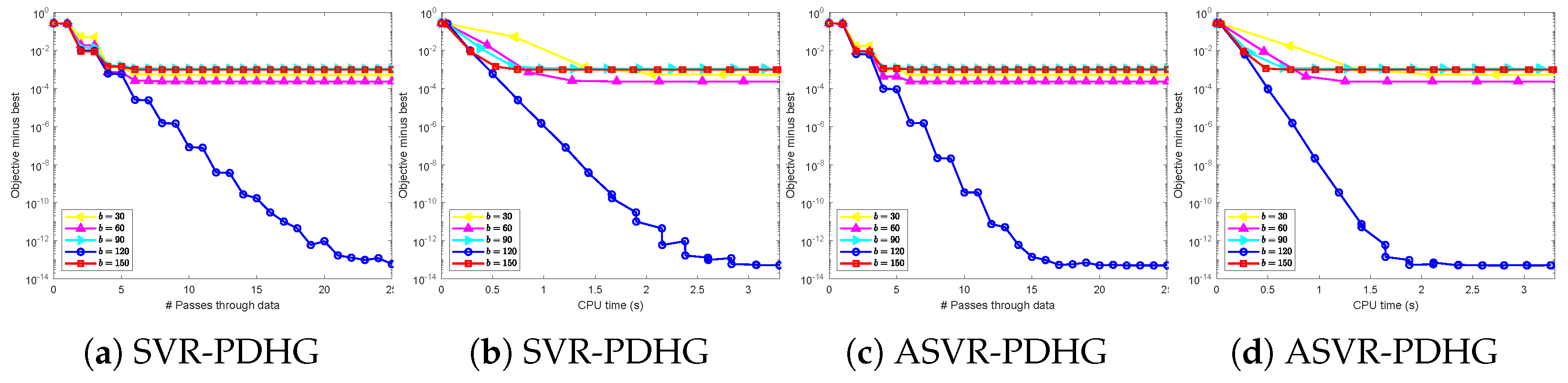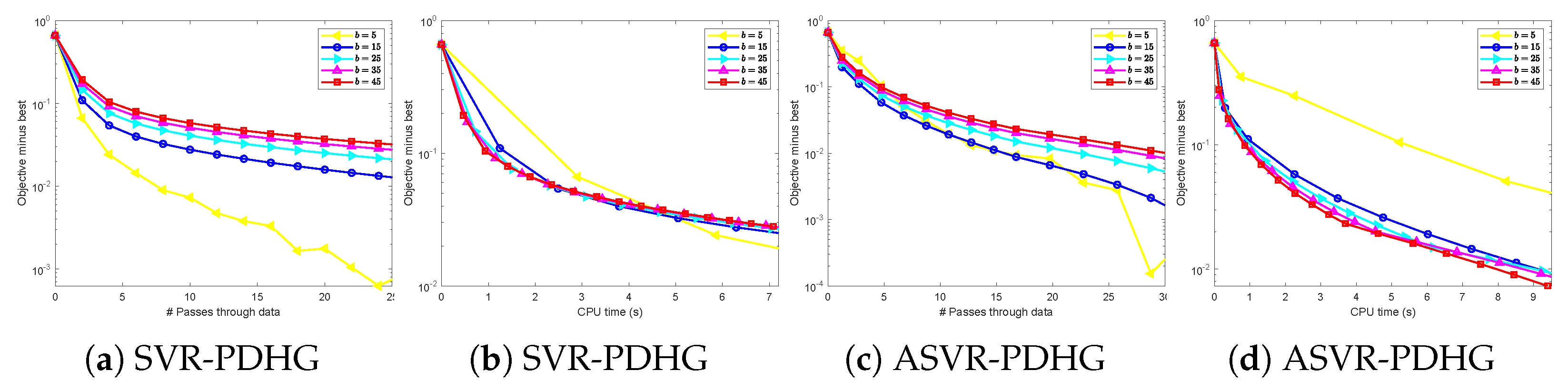As for the compared algorithms, we choose the same hyper-parameters as in the work [56] for ASVRG-ADMM, we tune the parameters as in the work [20] for SVRG-ADMM, and we also adopt the grid search method and choose the optimal step sizes $\eta =\rho =1$ for SVRG-PDFP. About mini-batch sizes, we choose them guided by theory and considering the trade-off between time consumption and reasonably good performance. Specifically, we test the performance of our algorithms under different mini-batch sizes, and the results are shown in Figure A1 and Figure A2 in Appendix B. According to Figure A1 and Figure A2, considering the trade-off between time cost and loss, we determine the mini-batch sizes $b=120$ for SC problems and $b=15$ for non-SC problems.

We first solve the following non-SC graph-guided fused Lasso problem and SC graph-guided logistic regression problem in Section 5.1, Section 5.2, Section 5.3 and Section 5.4:

$$\underset{x\in {\mathbb{R}}^d}{\min }\{{\displaystyle \frac{1}{n}}\sum _{i=1}^n{F}_i\left(x\right)+{\lambda }_1{\parallel Ax\parallel }_1\},\underset{x\in {\mathbb{R}}^d}{\min }\{{\displaystyle \frac{1}{n}}\sum _{i=1}^n\left(F_i\left(x\right)+{\displaystyle \frac{{\lambda }_2}{2}}{\parallel x\parallel }^2\right)+{\lambda }_1{\parallel Ax\parallel }_1\{,$$

(22)

where each $F_i\left(x\right)=log(1+exp(-c_i{a}_i^{\top }x))$ is the logistic loss on the feature–label pair $(a_i,c_i)$, ${\lambda }_1\ge 0$ and ${\lambda }_2\ge 0$ are two regularization parameters. And here, we set A as described in the work [57]. The ${\ell }_1$-norm regularized minimization can be converted into Problem (1) by setting ${\lambda }_1{\parallel Ax\parallel }_1={\max }_{{\parallel y\parallel }_{\infty }\le {\lambda }_1}\langle y,Ax\rangle$, where ${\parallel ·\parallel }_{\infty }$ is the maximum norm of a vector. Thus, Problem (22) can be converted into the following saddle-point problems, respectively:

$$\underset{x\in {\mathbb{R}}^d}{\min }\underset{{\parallel y\parallel }_{\infty }\le {\lambda }_1}{\max }\{{\displaystyle \frac{1}{n}}\sum _{i=1}^n{F}_i\left(x\right)+\langle y,Ax\rangle \},$$

(23)

$$\underset{x\in {\mathbb{R}}^d}{\min }\underset{{\parallel y\parallel }_{\infty }\le {\lambda }_1}{\max }\{{\displaystyle \frac{1}{n}}\sum _{i=1}^n\left(F_i\left(x\right)+{\displaystyle \frac{{\lambda }_2}{2}}{\parallel x\parallel }^2\right)+\langle y,Ax\rangle \}.$$

(24)

Here, the conjugate function $G^{*}\left(y\right)=0$. Then, we consider the general case $G^{*}\left(y\right)\ne 0$ in Section 5.5. Lastly, we solve the non-SC multi-task learning problem in Section 5.6.

5.1. Comparison of PDHG-Type Algorithms on Synthetic Datasets

In this subsection, to verify the advantages of our algorithms compared with PDHG-type algorithms, we first conduct experiments for solving Problems (23) and (24) on synthetic datasets. The method of generating a synthetic dataset is described below. Each sample $a_i$ is generated from i.i.d. standard Gaussian random variables and normalized according to $a_i={\displaystyle \frac{a_i}{\max \left\{a_i\right\}}}$, and the corresponding label is obtained by $c_i=\mathrm{sign}(a_i^{\top }{x}_0+{ϵ}_i)$, where the vector $x_0$ is generated from the d-dimensional standard normal distribution. The noise ${ϵ}_i$ also comes from the normal distribution with mean 0 and standard deviation 0.01. For Problem (23), we set ${\lambda }_1={10}^{-5}$, and for Problem (24), we set ${\lambda }_1={10}^{-5}$ and ${\lambda }_2={10}^{-2}$.

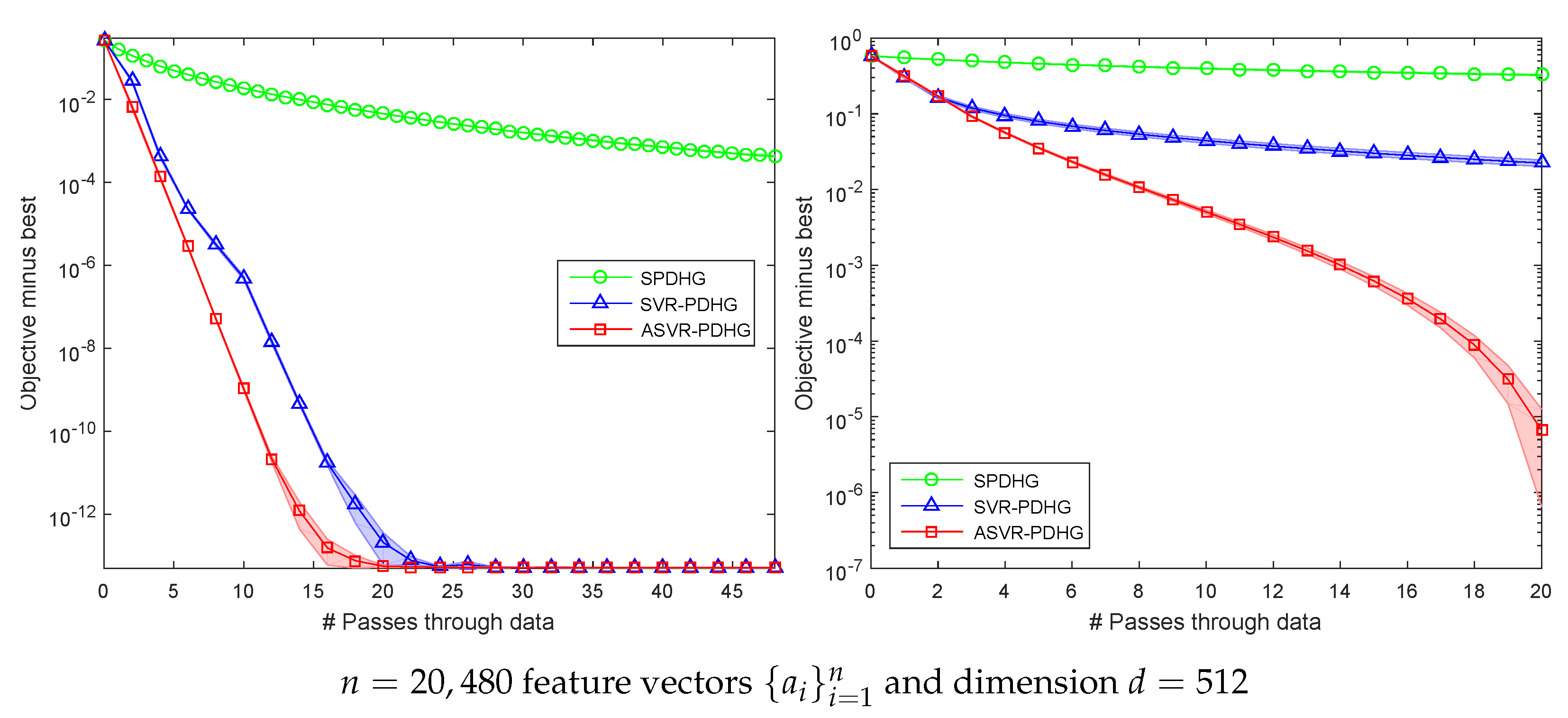
Figure 1 shows the comparison between our algorithms and SPDHG for solving SC and non-SC problems on a small-scale synthetic dataset. The experimental results imply that variance reduction methods including SVR-PDHG and ASVR-PDHG converge obviously faster than SPDHG, which verifies our algorithms improving the theoretical convergence rate. ASVR-PDHG converges much faster than SVR-PDHG in the non-SC setting, which verifies that the momentum acceleration step can significantly improve the convergence speed for solving non-SC problems. ASVR-PDHG performs better than SVR-PDHG in the SC setting, which demonstrates the superiority of momentum acceleration for solving SC problems.

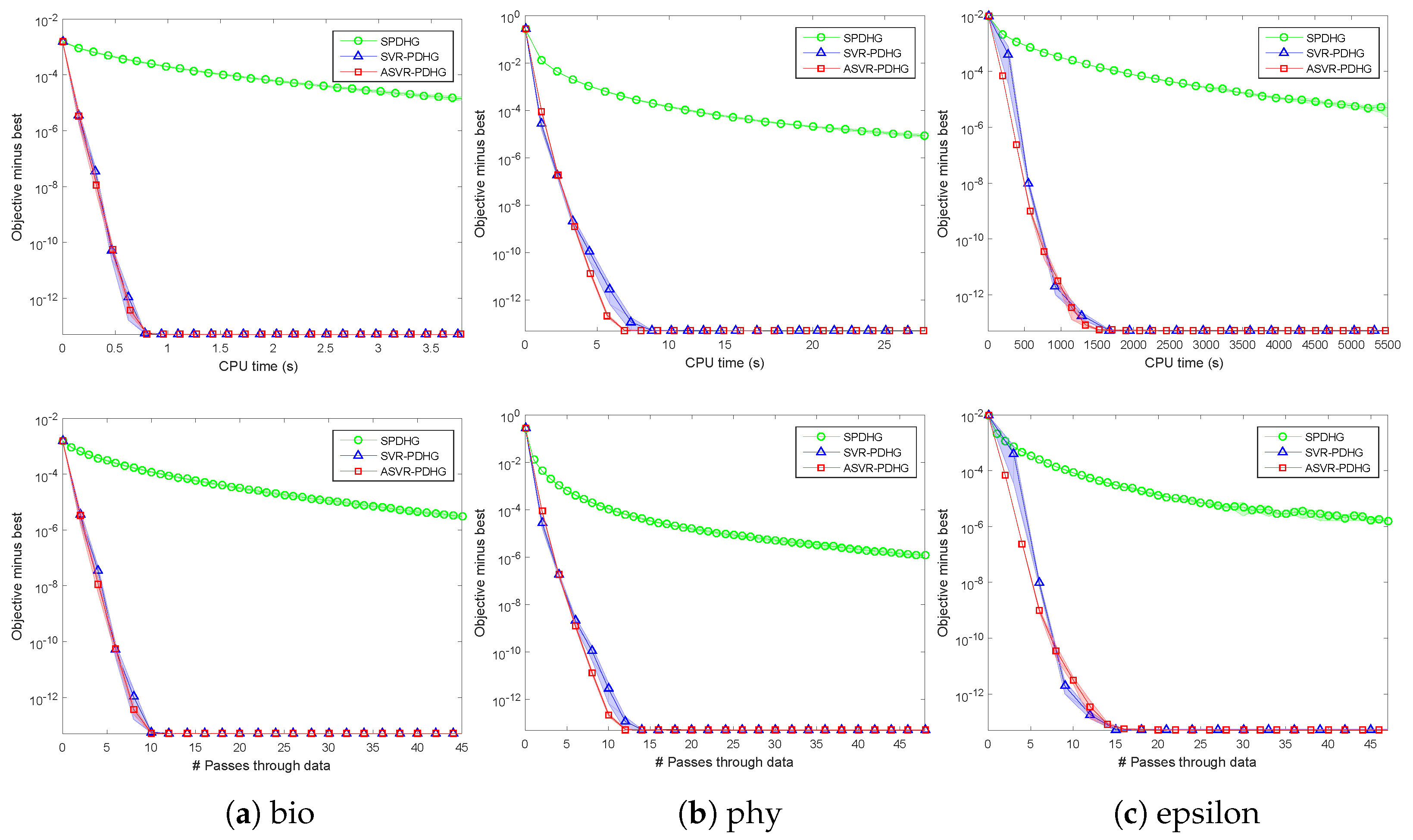
5.2. Comparison of PDHG-Type Algorithms on Real-World Datasets

To further verify the advantages of our algorithms compared with the SPDHG algorithm on real-world datasets, we also conduct experiments on bio, phy, w8a, epsilon, and epsilon_test datasets, which can be downloaded from the LIBSVM website (https://www.csie.ntu.edu.tw/~cjlin/libsvm/, accessed on 5 November 2021) and the KDDCUP website (http://osmot.cs.cornell.edu/kddcup/datasets.html, accessed on 5 November 2021). The detailed description of these datasets is shown in

Table 2. Some real-world datasets and their mini-batch sizes used in our experiments.

Datasets	# Training Samples	# Testing Samples	# Dimension	b (SC)	b (Non-SC)
bio	116,600	29,151	74	120	15
phy	40,000	10,000	78	120	15
epsilon	320,000	80,000	2000	120	15
w8a	39,800	9949	300	120	15
epsilon_test	80,000	20,000	2000	120	15

.

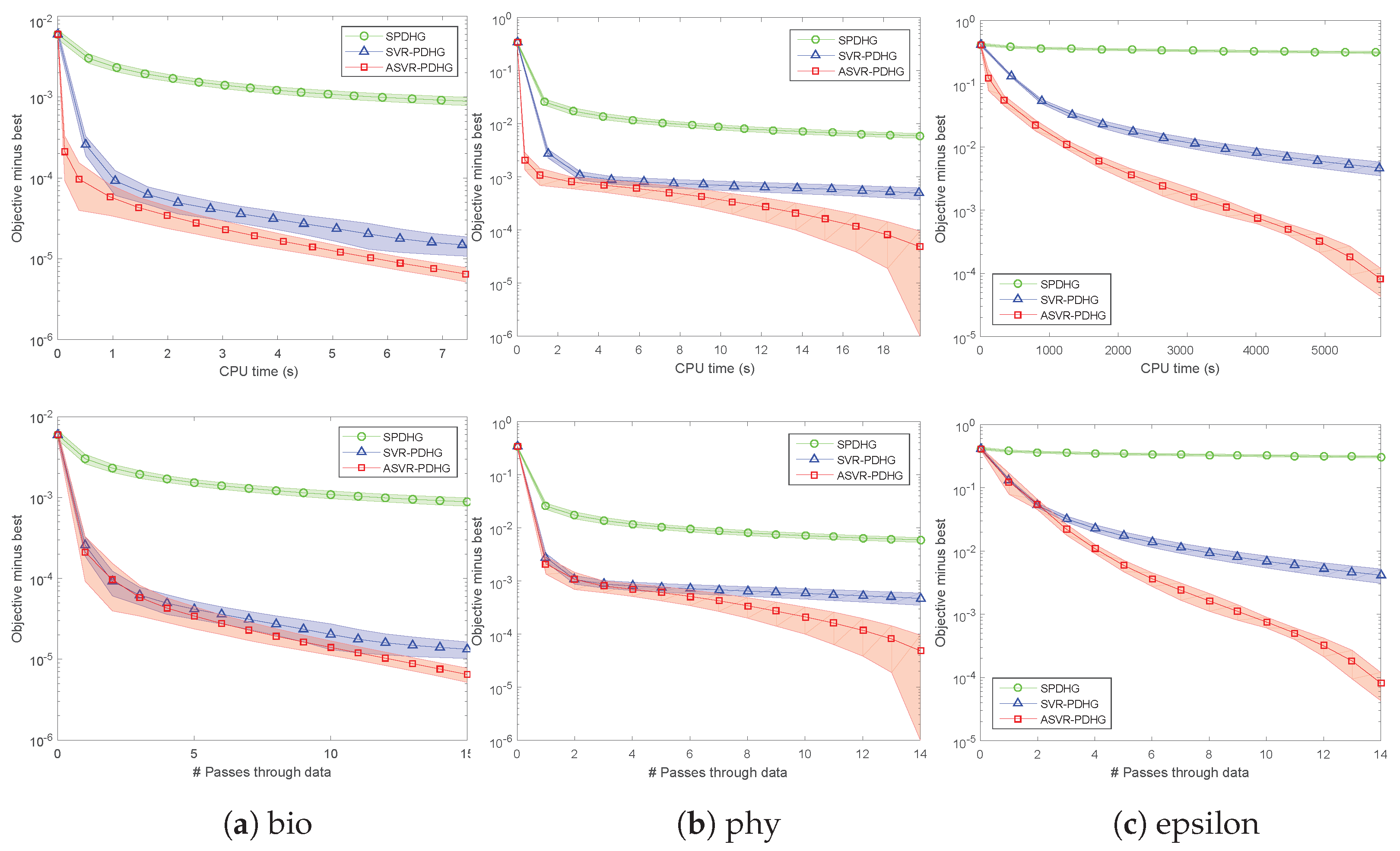
Due to similar experimental phenomena on the five real-world datasets in Table 2, we only report the results on the bio, phy, and epsilon datasets in this subsection. Figure 2 shows the experimental results of Algorithms 2 and 4 to solve the non-SC problem (23) with ${\lambda }_1={10}^{-5}$. All the experimental results show that our SVR-PDHG and ASVR-PDHG perform obviously better than their baseline, SPDHG. Moreover, our ASVR-PDHG consistently converges much faster than both SVR-PDHG and SPDHG in all the cases, which verifies the effectiveness of our momentum trick to accelerate the variance reduced stochastic PDHG algorithm.

As for SC objectives, Figure 3 shows the experimental results of SVR-PDHG and ASVR-PDHG on the three real-world datasets, where ${\lambda }_1={10}^{-5}$, and ${\lambda }_2={10}^{-2}$. It can be observed that SVR-PDHG and ASVR-PDHG are superior to the baseline, SPDHG, by a significant margin, in terms of their number of passes through data and CPU time, which also verifies our theoretical convergence results, i.e., linear convergence rate. Note that the standard deviation of the results of our methods is relatively small, which implies that our algorithms are relatively stable.

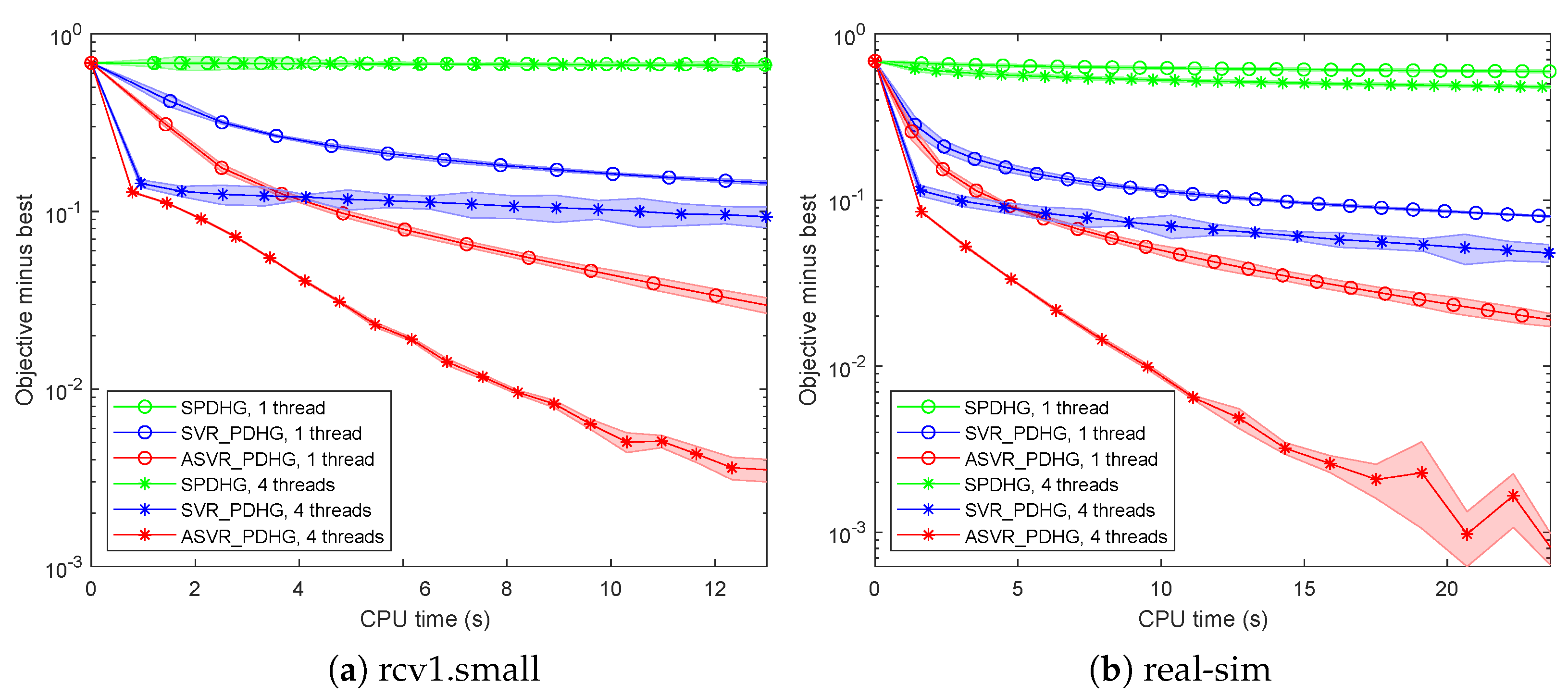
5.3. Sparse and Asynchronous Parallel Setting

We also conduct our algorithms in the sparse and asynchronous parallel settings. We consider $A=I$ in the non-SC Problem (23) to facilitate parallelism and select the regularization parameter ${\lambda }_1={10}^{-5}$. The sparse datasets rcv1.small and real-sim are used to test our algorithms, and we choose $D_{i_t}$ as in the work [50]. We choose the single-thread algorithm as the baseline and compare the performance of all the methods in terms of the running time. The parallel SPDHG is achieved by updating the support sets of vectors $x_t$ and $y_t$ in a parallel fashion by ourselves. All the algorithms under asynchronous parallel setting are implemented in C++ with a Matlab interface, and the experimental results are shown in Figure 4.

All the experimental results in Figure 4 show that our SVR-PDHG and ASVR-PDHG significantly outperform SPDHG in terms of running time on both one thread and four threads. Our ASVR-PDHG method achieves more than $3\times$ and $5\times$ speedup over our SVR-PDHG on one thread and four threads, respectively, which benefits from our momentum acceleration and adaptive epoch length strategy. Moreover, SVR-PDHG and ASVR-PDHG with four threads achieve more than $3\times$ speedup than those with one thread, respectively. These phenomena indicate that the linear extrapolation step, momentum acceleration trick, and adaptive epoch length strategy are also suitable for large-scale machine learning problems in the sparse and asynchronous parallel setting, and our asynchronous parallel algorithms achieve a speedup proportional to the number of threads.

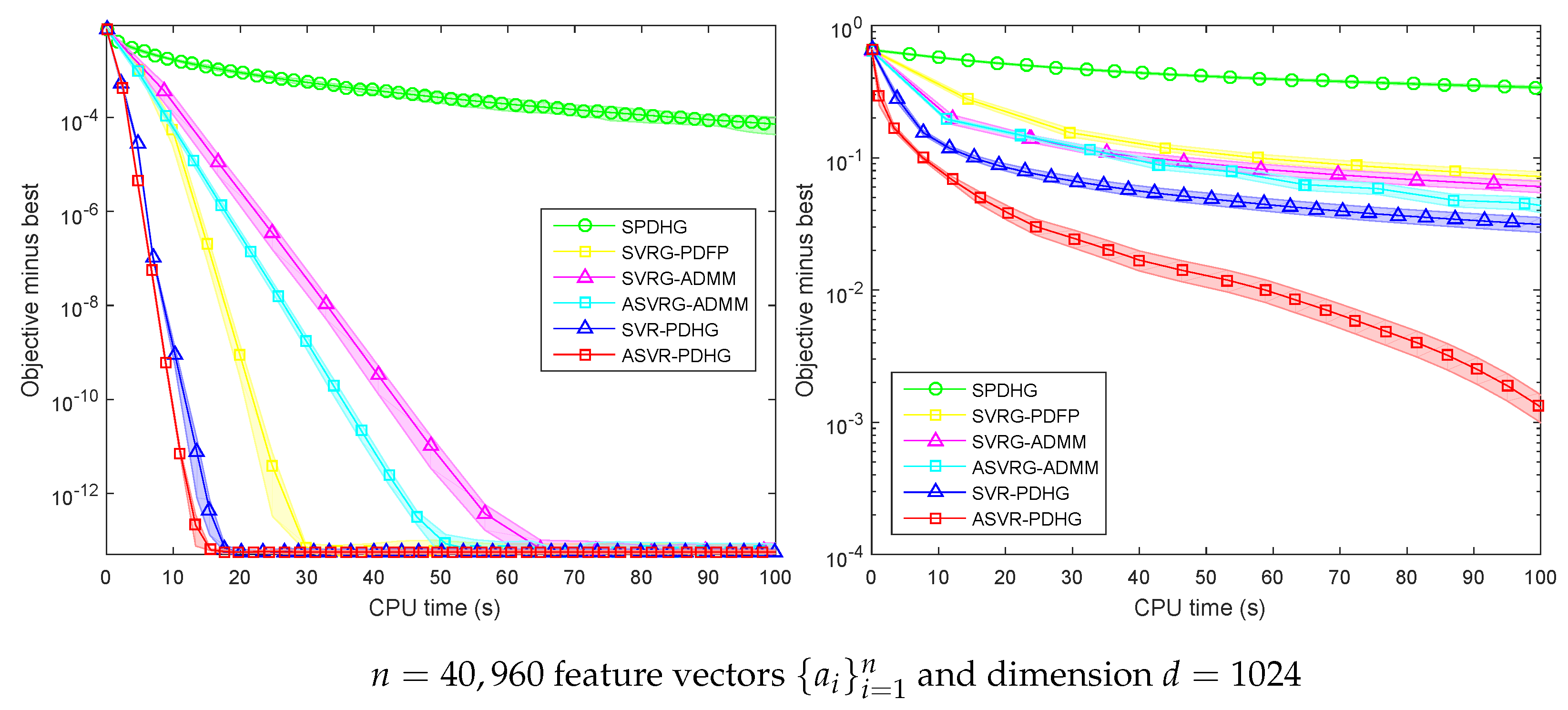
5.4. Compared with State-of-the-Art Stochastic Methods

To illustrate the advantages of our methods over SOTA methods, we further conduct some experiments on a large-scale synthetic dataset and real-world datasets. And we also set $b=120$ and $b=15$ for SC and non-SC problems, respectively.

Figure 5 shows the experimental results of SPDHG, SVR-PDHG, ASVR-PDHG, SVRG-ADMM, and ASVRG-ADMM on a larger synthetic dataset. It can be found that our algorithms (SVR-PDHG and ASVR-PDHG) converge significantly faster than SPDHG. For SC problems, SVR-PDHG and ASVR-PDHG achieve an average speedup of $3\times$ over SVRG-ADMM and ASVRG-ADMM, and $2\times$ over SVRG-PDFP. For non-SC problems, ASVR-PDHG achieves an average speedup of at least $4\times$ compared with other algorithms, which benefits from fewer variables, without Q, and the momentum acceleration technology.

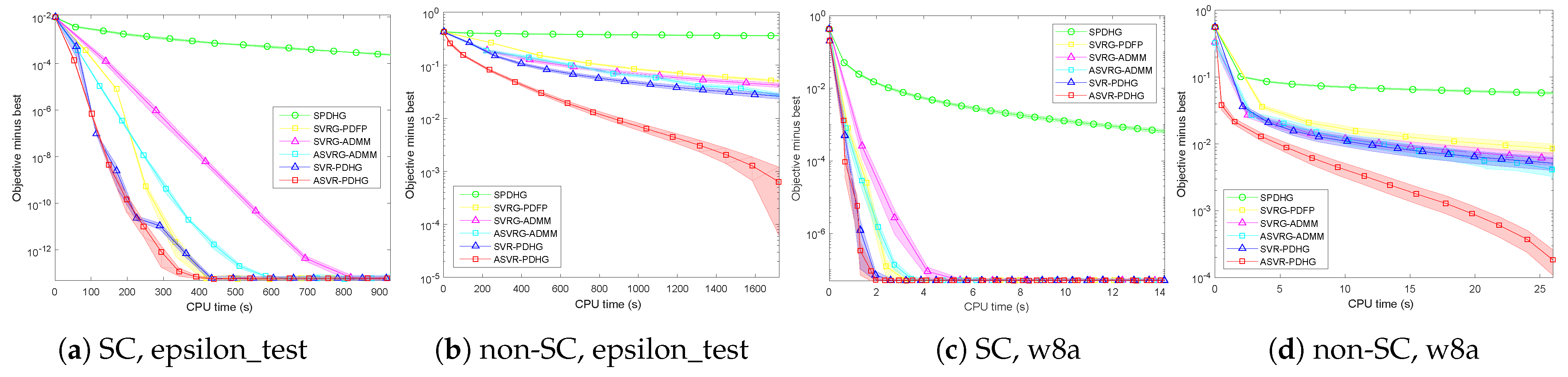
Due to limited space and similar experimental phenomenon on the five real-world datasets in Table 2, we only report the results on the epsilon_test and w8a datasets. Figure 6 shows the compared results. It can be seen that our ASVR-PDHG almost always converges much faster than the stochastic ADMMs in all the settings. For SC problems, although the linear convergence rate can be obtained by all the algorithms, our algorithms achieve an average speedup of $2\times$ over SVRG-ADMM and ASVRG-ADMM because we do not require Q of ADMM-type methods. Moreover, compared with SVRG-PDFP, our algorithms also converge significantly faster. For non-SC problems, our ASVR-PDHG achieves at least $3\times$ speedup over other stochastic algorithms.

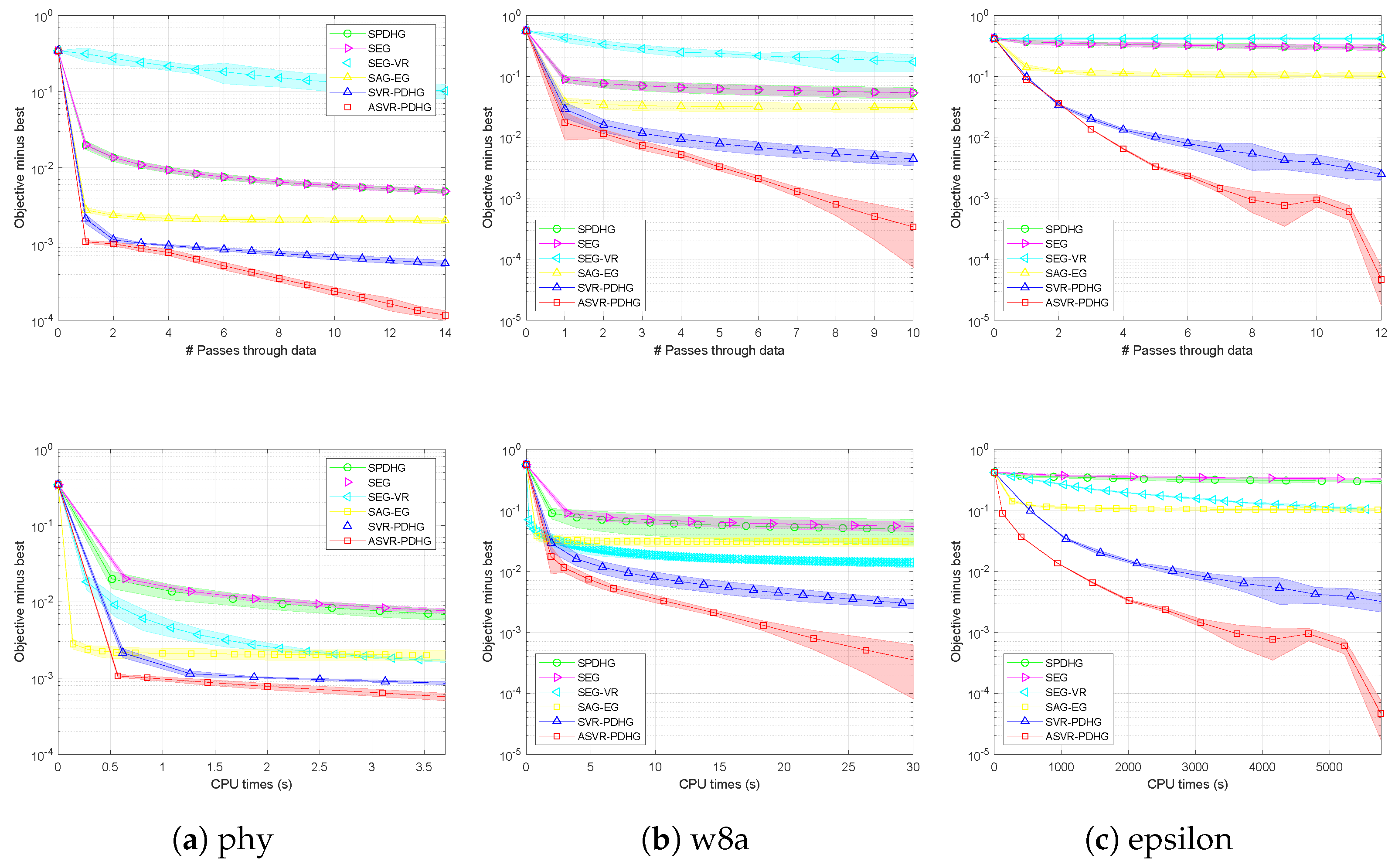
We also compare our methods with the famous extragradient (EG) methods such as stochastic EG [58] (SEG), stochastic AG-EG [59] (SAG-EG), and stochastic variance reduction EG [60] (SEG-VR) methods. We set the same initialization and choose the batch size and step sizes guided by theory, considering the trade-off between time consumption and accuracy, while observing reasonably good performance. The experimental results on the phy, w8a, and epsilon datasets are shown in Figure 7. From Figure 7, we can observe that our proposed methods still converge faster than EG-type methods. Especially for non-SC problems, our SVR-PDHG and ASVR-PDHG algorithms can achieve at least 6× and 7× speedup compared to EG-type methods, respectively, which benefit from the variance reduction and our momentum acceleration technology.

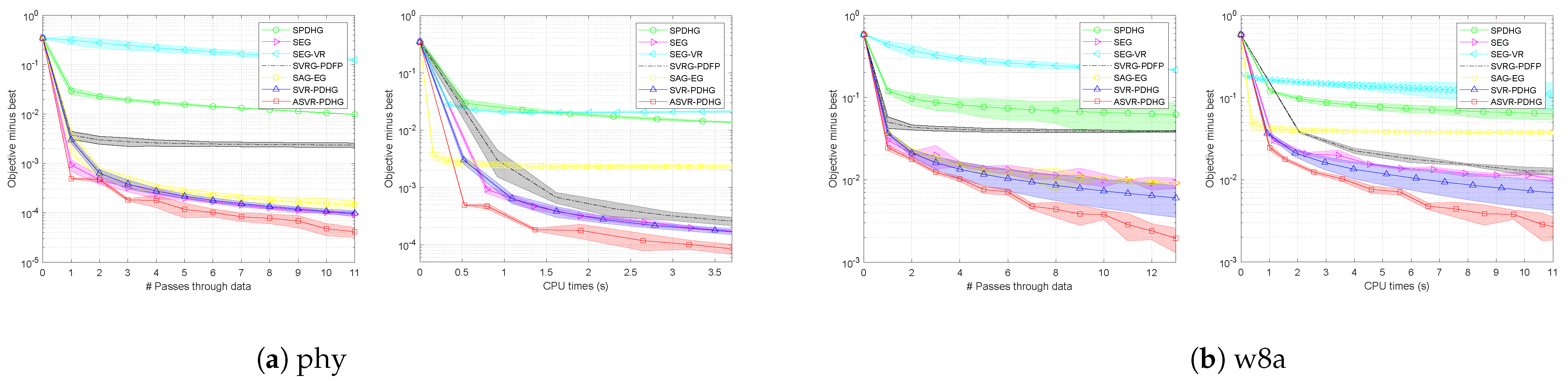
5.5. Comparisons of Primal–Dual Algorithms When $G^{*}\left(y\right)\ne 0$

We further conduct our algorithms to solve the general setting, i.e., $G^{*}\left(y\right)\ne 0$. We compare our methods and other primal–dual algorithms such as SEG [58], SAG-EG [59], SEG-VR [60], and SVRG-PDFP [46] methods when solving the logistic regression problem with ${\ell }_2$ regularization:

$$\underset{\mathbf{x}}{\min }{\displaystyle \frac{1}{n}}\sum _{i=1}^n{F}_i\left(x\right)+{\displaystyle \frac{\lambda }{2}}{\parallel x\parallel }^2.$$

(25)

Its primal–dual formulation is

$$\underset{x}{\min }\underset{y}{\max }{\displaystyle \frac{1}{n}}\sum _{i=1}^n{F}_i\left(x\right)+\lambda \langle x,y\rangle -{\displaystyle \frac{\lambda }{2}}{\parallel y\parallel }^2,$$

(26)

where $G^{*}\left(y\right):={\displaystyle \frac{\lambda }{2}}{\parallel y\parallel }^2$ and $\lambda \ge 0$ is a regularization parameter. We set the same initialization $(x_0,y_0)$ and batch size to compare all the methods. The convergence results are shown in Figure 8.

From Figure 8, it can be found that the experimental phenomenon is similar to the case of $G^{*}\left(y\right)=0$. Specifically, our SVR-PDHG algorithm performs sightly better than SEG and SVRG-PDFP methods and achieves a speedup of at least $6\times$ compared to other comparison methods. Our ASVR-PDHG algorithm further improves the convergence speed of our SVR-PDHG algorithm, which again verifies the effectiveness of our momentum acceleration technology.

5.6. Multi-Task Learning

In this subsection, in order to verify the advantages of our algorithms for solving the matrix nuclear norm regularized problem, we conduct the following multi-task learning experiments. Here, the multi-task learning model can be described as follows:

$$\underset{X}{\min }\sum _{i=1}^N{l}_i\left(X\right)+{\lambda }_1{\parallel X\parallel }_{*},$$

(27)

where $X\in {\mathbb{R}}^{d\times N}$, N is the number of tasks, $l_i\left(X\right)$ is the logistic loss on the i-th task, and ${\parallel ·\parallel }_{*}$ is the nuclear norm.

An auxiliary variable Y is introduced to solve the above model, and the original model can be transformed into the equality constrained problem ${\min }_X{\sum }_{i=1}^N{l}_i\left(X\right)+{\lambda }_1{\parallel Y\parallel }_{*}$, s.t. $X=Y$, which can be solved by stochastic ADMMs. In order to apply the primal–dual technique to solve this problem, the nuclear norm needs to be rewritten as ${\lambda }_1{\parallel X\parallel }_{*}={\max }_{\parallel X^{\prime }{\parallel }_2\le {\lambda }_1}\langle X^{\prime },X\rangle$, where ${\parallel ·\parallel }_2$ is the spectral norm of a matrix. In this way, the multi-task learning model can be formulated into a saddle-point problem as follows:

$$\underset{X}{\min }\underset{\parallel X^{\prime }{\parallel }_2\le {\lambda }_1}{\max }\sum _{i=1}^N{l}_i\left(X\right)+\langle X^{\prime },X\rangle .$$

(28)

Here, the conjugate function $G^{*}\left(X^{\prime }\right)=0$. This problem can be also solved by SPDHG, SVRG-PDFP, SVRG-ADMM, ASVRG-ADMM, and our algorithms.

We compare the stochastic ADMMs, SVRG-PDFP, and our algorithms on a dataset, 20newsgroups (available at https://github.com/jiayuzhou/MALSAR/tree/master/data, accessed on 5 November 2021), and set ${\lambda }_1={10}^{-5}$ and the mini-batch size $b=15$ for each task. The training loss (i.e., the training objective value minus the minimum value) and test error are shown in Figure 9. It can be observed that ASVR-PDHG significantly outperforms other algorithms in terms of convergence speed and test error.

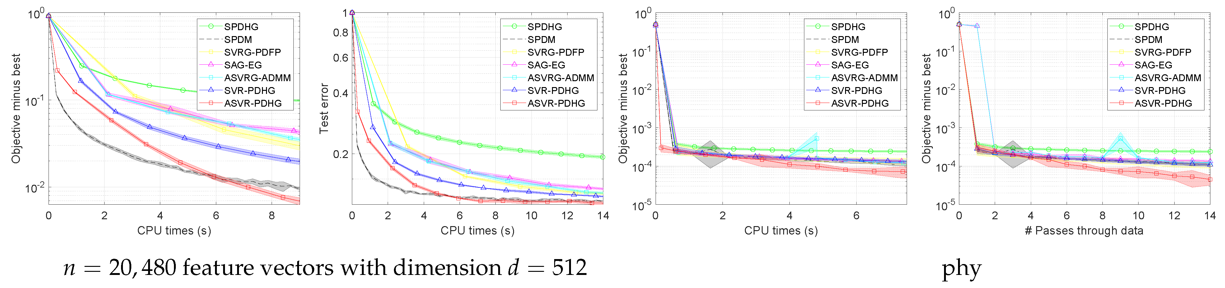
5.7. Non-Convex Support Vector Machines

We also compare the related methods on the Support Vector Machine (SVM) problem. Given a training set $S={(a_i,c_i)}_{i=1}^n$, the non-convex ${\ell }_1$-norm penalized SVMs minimize the following penalized hinge loss function:

$$\underset{x}{\min }{\displaystyle \frac{1}{n}}\sum _{i=1}^n\max \{0,1-c_i{x}^{\top }{a}_i\}+\lambda {\parallel Ax\parallel }_1.$$

(29)

In the same way, the SVMs can be formulated into a saddle-point problem:

$$\underset{x}{\min }\underset{{\parallel y\parallel }_{\infty }\le \lambda }{\max }{\displaystyle \frac{1}{n}}\sum _{i=1}^n\max \{0,1-c_i{x}^{\top }{a}_i\}+\langle y,Ax\rangle .$$

(30)

We compare the ASVRG-ADMM, SVRG-PDFP, SAG-EG [59], and SPDM [61] algorithms on a synthetic dataset and the phy dataset, and set $\lambda ={10}^{-5}$ and the mini-batch size $b=15$. Regarding other hyper-parameters, we choose them guided by theory and considering the trade-off between time consumption and reasonably good performance. The experimental results are shown in Figure 10. It can be found that when solving non-convex problems, our ASVR-PDHG algorithm can still maintain a certain advantage.

Limitations. Our algorithms can be proved to achieve an advanced convergence rate under the convex assumption. For the non-convex problems, although our algorithms have unknown convergence properties, they achieve better experimental performance than some state-of-the-art methods as shown in Figure 10. As for solving complex non-convex problems such as training deep networks, the gradient calculation and acceleration steps may increase computational cost, but since the batch size can be chosen to be $b=1$ and only vector addition operations are performed, the computational cost will not increase too much and will still be smaller than the ADMM-type algorithms. We will study the convergence properties of non-convex primal–dual problems in future work.

6. Conclusions and Future Work

In this paper, we proposed a stochastic primal–dual hybrid gradient method with variance reduction (SVR-PDHG) and an accelerated variant (ASVR-PDHG) for saddle-point problems. Compared with stochastic ADMMs, our algorithms have simpler structures. A new adaptive epoch length strategy was proposed to remove the extra boundedness assumption for non-SC problems. We theoretically analyzed the linear convergence properties of our methods without the strong convexity of $G^{*}(·)$ for SC problems. In particular, we rigorously proved that the convergence rates of SVR-PDHG and ASVR-PDHG are $\mathsf{𝒪}(1/S)$ and $\mathsf{𝒪}(1/S^2)$ for non-SC problems, respectively. As a by-product, we extended our algorithms to asynchronous parallel settings for non-SC problems and experiments verify that our parallel algorithms are suitable for large-scale sparse non-SC machine learning problems. Finally, various experimental results verified that our ASVR-PDHG consistently converges much faster than the existing stochastic methods.

Besides the machine learning problems mentioned above, we can extend our algorithms to solve image processing problems [34] and differentially private problems [62,63] in future work. Another interesting direction for future work is the research of the theoretical properties of our asynchronous parallel primal–dual algorithms.