High-Performance Deployment Operational Data Analytics of Pre-Trained Multi-Label Classification Architectures with Differential-Evolution-Based Hyperparameter Optimization (AutoDEHypO)

Abstract

This article presents a high-performance-computing differential-evolution-based hyperparameter optimization automated workflow (AutoDEHypO), which is deployed on a petascale supercomputer and utilizes multiple GPUs to execute a specialized fitness function for machine learning (ML). The workflow is designed for operational analytics of energy efficiency. In this differential evolution (DE) optimization use case, we analyze how energy efficiently the DE algorithm performs with different DE strategies and ML models. The workflow analysis considers key factors such as DE strategies and automated use case configurations, such as an ML model architecture and dataset, while monitoring both the achieved accuracy and the utilization of computing resources, such as the elapsed time and consumed energy. While the efficiency of a chosen DE strategy is assessed based on a multi-label supervised ML accuracy, operational data about the consumption of resources of individual completed jobs obtained from a Slurm database are reported. To demonstrate the impact on energy efficiency, using our analysis workflow, we visualize the obtained operational data and aggregate them with statistical tests that compare and group the energy efficiency of the DE strategies applied in the ML models.

1. Introduction

High-performance computing (HPC) continues to advance and to provide important infrastructure and a backbone for the scientific community, industry, and beyond, making efficient utilization highly important for both environmental sustainability and cost efficiency [1,2]. Despite the increasing availability of automated ML (AutoML) frameworks, most existing tools prioritize and maximize the performance (accuracy) and neglect other important objectives such as energy efficiency (EE) and resource usage and optimization, which are key factors in large-scale HPC environments and beyond [3,4]. Therefore, the enforcement of sustainable and energy-efficient solutions, including the utilization and optimization of computational resources, now plays a key role in reducing operational financial costs and minimizing environmental impacts [1,3]. Due to the broad accessibility of computational resources for HPC, the scientific community with the myriad of application areas and diverse expertise from different fields, can deploy and run their workflows [5,6]. As their needs, demands, and complexity grow, running data-intensive and parallel workflows involves both different and heterogeneous architectures and the resources of state-of-the-art systems [6,7,8]. Such heterogeneous architectures introduce challenges in workload scheduling, as there are many unknowns and uncertainties  [2,9]. However, despite the optimization capabilities and advances, most AutoML frameworks do not incorporate schedulers such as Slurm, nor do they provide support for energy monitoring, as their main focus is on improving ML model performance (accuracy) and ignore constraints such as EE, utilization, and resource allocation [3,4,10]. To address these challenges, adjusted and tailored frameworks that support sustainable and cost-efficient HPC environments are needed. Therefore, this article presents a high-performance-computing (HPC) differential-evolution-based automatic hyperparameter optimization workflow (AutoDEHypO) for energy efficiency and operational data analytics using multiple graphics processing units (GPUs), and this is deployed on the petascale EuroHPC supercomputer Vega [11]. Our proposed method is capable of determining how energy-efficient the differential evolution (DE) algorithm and ML models perform. The proposed AutoDEHypO workflow considers both their achieved accuracy and the utilization of computing resources, such as elapsed time and consumed energy; it collects runtime data through Slurm within the HPC environment, and the job allocation may impact the obtained results. Moreover, resource consumption leads to inefficient workloads, waste of computational resources, the consumption of a project quota, longer queue times, and postponement of scientific research [12]. Since Slurm dynamically schedules jobs to available, unutilized, or idle nodes within the cluster queue, proper adjustments in job submission may lead to faster allocation and faster attainment of the required job results [13]. We aim to develop the ability to operate within the constraints that Slurm users have and determine whether statistical deviations will be significant. Thus, we prepared our environment for the deployment of the AutoDEHypO workflow, where we ensured consistent resource allocation across the submitted job scripts with a Slurm script (SBATCH). Furthermore, this setup includes supervised machine learning (ML) and multi-label classification and allows for applicable optimization for aspects of hyperparameters that could be affected [14]. We chose the recent parallel implementation of the DE algorithm [15], which parallelizes the population operations in an algorithm that was initially introduced by Storn and Price in 1995 [16]. While DE provides a favorable trade-off and balance between accuracy and energy efficiency (EE) in the context of HPC [17], it additionally offers several advantages over other optimization algorithms, such as efficient and faster convergence, suitability and adaptability in a variety of different environments and optimization problems, global optimization, parallelization, scalability, energy optimization, and the possibility for combination and complementarity with different algorithms and techniques due to available implementations and integrations [16,18,19,20,21]. Furthermore, DE is suitable for the given optimization problem, as it can be used for optimizing nonlinearities in data, such as ML-related input/output data within the workflow, and it can be adapted to other use cases and problems [19]. Data are gathered from system scheduling and historical data; resource allocation and job execution times make it difficult to provide prediction and optimization [16,19,20,21]. In the evaluation phase of our experiment, we used basic ML metrics [14]. During the deployment of individual jobs on multiple GPUs in our experiment, we examined the efficiency of a chosen ML model and DE algorithm according to the accuracy [14]. DE functions and strategies show distinct behavior, and this has not yet been extensively measured or optimized within the context of EE and system resource management in HPC environments [20,22,23]. Data on the consumption of resources of individual jobs were obtained from the Slurm database of completed jobs, with energy consumption data being reported for the whole node by Intelligent Platform Management Interface (IPMI) sensors [13,24]. Based on the results of the computations, aggregated statistics were calculated, along with corresponding post hoc procedures and visualizations, to evaluate the efficiency of the combined ML model and the applied DE strategy.

1.1. Problem Statement and Objective

This work addresses the challenge of optimizing machine learning (ML) models in high-performance computing environments by balancing ML accuracy, energy consumption, and resource utilization. To address these challenges, we propose AutoDEHypO, a differential-evolution-based workflow that is specifically designed for energy-monitored hyperparameter optimization. The specific problem stated for this study consists of considering some key limitations, such as inefficient utilization of computational resources during job allocation, extended queue times, and lack of integration with HPC environments and schedulers such as Slurm. The limitations of existing workflows and frameworks are that they mostly focus on a single objective, such as ML performance or integration within HPC environments, and do not necessarily contribute to the sustainability and cost-effectiveness of HPC environments [25,26]. Therefore, we are interested in analysis of the consumption of resources and when the consumed energy and other resources can lead to different ML performance and configurations.

1.2. Main Contributions

The main contributions of this article are as follows:

• We propose AutoDEHypO, a high-performance-computing differential-evolution-based automatic hyperparameter workflow designed to optimize the performance of ML models for energy efficiency and operational data analytics in HPC environments.
• We deploy the AutoDEHypO workflow on the EuroHPC Vega system, utilizing multiple GPUs and Slurm scheduling and submission to execute a specialized fitness function for ML.
• We applied and evaluated this workflow on supervised ML and multi-label classification using the CIFAR10 and CIFAR100 datasets [27].
• We collected runtime data through Slurm within the HPC production environment.
• We evaluated the efficiency of a chosen ML model and DE algorithm strategies according to the ML accuracy and energy efficiency, dependent on ML model architecture, datasets, and resource consumption within the HPC environment.
• We performed aggregated statistical analyses, along with the corresponding post hoc procedures, and validated the collected data using visualizations by evaluating efficiency of combined ML models and applied DE strategies.
• We identified significant differences in key metrics and laid the ground for future work on sustainability and cost-effectiveness using AutoDEHypO.

The following sections of this article are organized as follows. Section 2 provides an overview of the related work and existing methods. Section 3 provides a set of proposed methods. Section 4 provides the experimental results. Section 5 presents our conclusion and future work.

2. Related Work and Existing Methods

The integration of machine learning (ML) with monitoring and operational data analytics (MODA) is a step towards enhancing operational efficiency, and DE is being utilized to run DE fitness functions and enhance model performance through hyperparameter optimization and other techniques [28]. Furthermore, automated machine learning (AutoML) automates workflows and reduces manual effort [12]; here, the effectiveness of an ML model is evaluated using fundamental ML evaluation metrics, non-parametric tests, post hoc procedures, and visualizations [14]. Despite the improvements, there is still a trade-off between accuracy and energy efficiency [14]. Moreover, checkpoint, restart, and predictive models provide additional robustness and project quotas for allocated computational resources. The following subsections, therefore, describe these topics in the order in which they were mentioned here.

2.1. Machine Learning

Machine learning (ML) is used to discover patterns, make predictions, provide automation, and generate useful knowledge from datasets [29]. Several types of such discoveries have been made, through methods such as classification, regression, segmentation, clustering, error detection, sequence analysis, and others [29]. The design of layers (how they are connected and structured) represents the architecture of a model, while the trained version (system) represents an ML model itself [29]. Furthermore, in the context of learning, there is supervised machine learning and unsupervised machine learning [29]. In ML, patterns are identified within a dataset, and thus the model wants to connect attributes and classes—for example, through classification—with a focus on similarities on the one hand; on the other hand, unsupervised machine learning focuses on identifying underlying structures without a target attribute, such as segmentation [29].

In ML, optimization algorithms are used to improve results—specifically, losses within a selected space [14,30]. With the help of an ML algorithm, hyperparameters can be adjusted and optimized even before the learning phase [14]. The hyperparameters of ML are the configuration variables of ML methods [14]. Some of the most widely used optimization methods are grid search, random search, cross-validation, and Bayesian optimization [30,31]. The execution time of a manual search can be significantly longer due to the complexity of ML models and neural networks within their limits, and as a result, such a search uses significantly more computational resources [8,32].

A convolutional neural network (CNN) is suitable for processing patterns within images, processing video content, performing face recognition, processing medical data, and more. A CNN uses a filter, converts pixels into numerical values in the first layer, and processes or teaches them to recognize and analyze data with the help of subsequent layers [33].

Recurrent neural networks (RNNs) use a mechanism for storing information from previous states and process and interpret it, making them more suitable for processing when the data are structured and in some kind of sequence. They are used in areas such as natural language processing (NLP) and speech and handwriting recognition [34].

The complexity and efficiency of the model may be defined by the architecture design and structure of the NN, the layers, and their connectivity, including the number of layers, the framework, the model size, the  optimization that is applied, the input data, and more [8,35]. The efficiency and emergence of smaller ML models, which are also referred to as language models [36], may play a key role, as they are easier to manage and provide flexibility, allowing faster implementation of changes with fewer computational resources [37,38].

Multi-label classification is a type of supervised machine learning that enables each instance to be associated with multiple labels, and it differs from conventional single-label classification, where each instance can be associated with a single label [14,39]. Fine-tuning and other optimization techniques can be applied to hyperparameters, which will have an effect and improve the performance of a model [14,30]. Evaluation of progress and performance is performed using a metric (M). There are some fundamental ML metrics, such as the accuracy, precision, recall, and F-measure; in addition, metrics can be aggregated with possible prediction outcomes, e.g., total (T), true positive ($TP$), true negative ($TN$), false positive ($FP$), and false negative ($FN$), as presented in [14].

• Accuracy (A) [14]:

  $$M={\displaystyle \frac{TP+TN}{TP+TN+FP+FN}}$$

  (1)
• Precision (P) [14]:

  $$M={\displaystyle \frac{TP}{TP+FP}}$$

  (2)
• Recall (R) [14]:

  $$M={\displaystyle \frac{TP}{TP+FN}}$$

  (3)
• F-Measure ($F_1$) [14]:

  $$F_1=2\times {\displaystyle \frac{P\times R}{P+R}}$$

  (4)
• Metric Aggregation [14]:

  $$M={\displaystyle \frac{A+P+F_1+R}{T}}$$

  (5)

2.2. Monitoring and Operational Data Analytics

Monitoring and operational data analytics (MODA) in high-performance computing can be applied to broad standards and practices for the integration, collection, storage, processing, monitoring, visualization, and analysis of system data [28]. MODA is used with the goal of helping end users make informed decisions about information collected on their system through hardware power monitoring and management tools such as IPMI, RAPL, and others [40]. These tools provide information such as sensor data, usage of generic resources, job status, memory, wall time, job and node utilization, power consumption per job, nodes, blades, racks, clusters, data centers, cluster occupancy, billing, and more to be leveraged in many ways [13,28]. Furthermore, MODA can be applied and extended to either an active or a passive setup, which depends on the requirements, potential benefits, and contributions that it may offer [40]. An active setup actively influences the runtime operations, while on the other hand, a passive setup passively monitors, gathers, and collects data without affecting the runtime operations [40]. To enhance the impact of ML and gather insights into data, MODA may be used to monitor energy consumption, improve job efficiency, and improve the ML design for EE by providing real-time feedback mechanisms for adaptive and dynamic changes within ML operations, ML optimization suggestions such as predictions in ML models, or even operational insights to resolve issues by proactively predicting potential trends and patterns within ML operations [9,40,41]. Such an analysis could identify trade-offs and bring the right balance, resulting in potential reductions in the consumption of resources and bringing sustainability and EE into view [28]. Furthermore, MODA offers multiple opportunities and can potentially contribute to EE due to the possibility of monitoring energy and detecting significant differences, preventing potential issues and anomalies, finding potential root causes, detecting security vulnerabilities and malware, and providing improvements in performance, reliability, throughput, and beyond [42]. Using HPC Vega [11], the topics of MODA, including energy monitoring, operational efficiency, and optimization of HPC workloads, were investigated and recently addressed in [43].

2.3. Differential Evolution

The differential evolution (DE) algorithm is a population algorithm and was introduced by Storn and Price in 1995 [44]. DE has been used successfully in the field of optimization of numerical functions and in applications to real problems within different domains [16]. The original DE has a main evolutionary loop through which, with the help of the key and basic operators presented in Figure 1, such as initialization, mutation, crossover, and selection, the final result can be gradually improved soon after each generation by repeating these operators until the end [45]. From its introduction to the present, interest in DE has increased year on year [16,44]. Thus, DE has been developed, improved, and applied to a variety of real-world problems within multidisciplinary domain areas, such as electrical and energy systems, artificial neural networks, manufacturing and pperation research, robotics and advanced systems, pattern recognition, image processing, bioinformatics and biomedicine, electrical engineering, and others, as presented in several articles [16,46,47,48,49]. Those mechanisms can be used to make the selection process easier [50]. DE provides a favorable trade-off and balance between accuracy and energy efficiency within HPC environments and beyond [17]. Additionally, DE offers several advantages over other optimization algorithms, such as efficient and faster convergence and suitability and adaptiveness in a variety of different environments and optimization problems; often, it provides better results than other algorithms [18,51,52,53]. Furthermore, DE can be used for nonlinear, nondifferentiable, and multi-objective problems [16]. It provides robustness in complex and multidimensional spaces, global optimization in complex spaces, parallelization, scalability in high-dimensional problems, and energy optimization and distribution without compromising throughput [16,18]. It can be integrated with penalty functions and other methods to handle constraints, and it can be combined and used to complement different algorithms and techniques due to its easy implementation and integration [16,21]. Last but not least, it is being extensively researched, and constant improvements to the algorithm are being made [16,18,21].

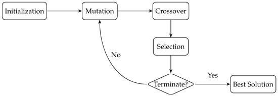
Figure 1. This figure shows the basic steps of differential evolution, including initialization, crossover, mutation, selection, and condition (loop). Until the stopping condition is met, i.e., max generations or convergence, the mutation, crossover, and selection processes are repeated over generations; then, the best solution that is found is provided [54].

2.3.1. Differential Evolution Operators

In DE [20], the following operators are used as highlighted in Figure 1.

First, the search space is initialized, and all search variables are randomly populated in the search space for a population of $\mathit{NP}$ vectors defined with a dimension; then, the parameter vectors may change over different iterations [16]. The sequential number of the current generation [16] is denoted by t, the optimization search dimension size is denoted with d, and $i\in \{1,2,\dots ,\mathit{NP}\}$ denotes a population vector index [16].

$${\mathbf{x}}_i^{\left(t\right)}=({x_{i,1}}^{\left(t\right)},{x_{i,2}}^{\left(t\right)},\dots ,{x_{i,d}}^{\left(t\right)}).$$

(6)

Within this initialization stage the vector must be composed of the following components within interval limits for minimum and maximum [16]:

$${x_{i,j}}^{\left(0\right)}=x_{\min ,j}+{\mathrm{rand}}_{[0,1];i,j}(x_{\max ;j}-x_{\min ;j}).$$

(7)

During mutation, after the first step is completed, the algorithm selects donor and mutated vectors for each population individual [55]. The following strategies are used most often (interval from 1 to $\mathit{NP}$), where ${\mathbf{x}}_i^{\left(t\right)}$ denotes the target vector, ${\mathbf{v}}_i^{\left(t\right)}$ denotes the mutant vector, ${\mathbf{x}}_{\mathrm{best}}^{\left(t\right)}$ denotes the best individual in the population, $R_j^i$ denotes random indexes that are mutually different and different from i, F denotes the mutation scaling factor, and t denotes the current generation [16,55,56]

• DE/rand/1: A random vector is chosen as the basis, and a one-sided weighted difference (vector) composed of two other random vectors is added to it.

  $${\mathbf{v}}_i^{\left(t\right)}={{\mathbf{x}}_{R_{1^i}}}^{\left(t\right)}+F({{\mathbf{x}}_{R_{2^i}}}^{\left(t\right)}-{{\mathbf{x}}_{R_{3^i}}}^{\left(t\right)}),$$

  (8)
• DE/best/1: The current best random vector is used as the basis, and an additional random difference (vector) is added to it.

  $${\mathbf{v}}_i^{\left(t\right)}={{\mathbf{x}}_{\mathrm{best}}}^{\left(t\right)}+F({{\mathbf{x}}_{R_{1^i}}}^{\left(t\right)}-{{\mathbf{x}}_{R_{2^i}}}^{\left(t\right)}),$$

  (9)
• DE/current-to-best/1: For an individual vector to mutate with the best vector, one random difference (vector) is added.

  $${\mathbf{v}}_i^{\left(t\right)}={\mathbf{x}}_i^{\left(t\right)}+F({{\mathbf{x}}_{\mathrm{best}}}^{\left(t\right)}-{\mathbf{x}}_i^{\left(t\right)})+F({{\mathbf{x}}_{R_{1^i}}}^{\left(t\right)}-{{\mathbf{x}}_{R_{2^i}}}^{\left(t\right)}),$$

  (10)
• DE/rand/2: A random vector is chosen as the basis, and two independent differences (vectors) of four random vectors are added to it.

  $${\mathbf{v}}_i^{\left(t\right)}={{\mathbf{x}}_{R_{1^i}}}^{\left(t\right)}+F({{\mathbf{x}}_{R_{2^i}}}^{\left(t\right)}-{{\mathbf{x}}_{R_{3^i}}}^{\left(t\right)})+F({{\mathbf{x}}_{R_{4^i}}}^{\left(t\right)}-{{\mathbf{x}}_{R_{5^i}}}^{\left(t\right)}),$$

  (11)
• DE/best/2: The current best random vector is used as the basis, and  two random differences (vectors) of four random vectors are added to it.

  $${\mathbf{v}}_i^{\left(t\right)}={{\mathbf{x}}_{\mathrm{best}}}^{\left(t\right)}+F({{\mathbf{x}}_{R_{1^i}}}^{\left(t\right)}-{{\mathbf{x}}_{R_{2^i}}}^{\left(t\right)})+F({{\mathbf{x}}_{R_{3^i}}}^{\left(t\right)}-{{\mathbf{x}}_{R_{4^i}}}^{\left(t\right)}).$$

  (12)

In the crossover phase, the donor vector crosses with the targeted vector [16]. The two most commonly used methods of crossing are exponential and binomial [16], and there are a few other combinations of mutation and crossover strategies in the original DE algorithm [20,55], namely, the  DE/rand/1/exp, DE/current-to-best/1/exp, DE/best/1/exp, DE/current-to-best/1/bin, DE/rand/2/exp, and DE/best/2/exp strategies. Exponential crossover works by choosing a random number within the size of the dimension {1, 2, …, d}. The target vector is then crossed with the donor vector [16]. The binomial crossover generates a number from interval $[0,1]$ for each dimension randomly and compares it to crossover value [16], in order to exchange components, or also exchange the component at random index $j=K$.

$${{\mathbf{u}}_{i,j}}^{\left(t\right)}=\left\{\begin{array}{cc}{{\mathbf{v}}_{i,j}}^{\left(t\right)}& \mathrm{if}j=K\mathrm{or}{\mathrm{rand}}_{[0,1];i,j}\le Cr,\\ {{\mathbf{x}}_{i,j}}^{\left(t\right)}& \mathrm{otherwise}.\end{array}\right.$$

(13)

In selection, survival to the next generation for both vectors, i.e., the target and the trial vector, is determined [16]. If the condition is met, the target vector is simply replaced according to the strategy chosen for the next generation; otherwise, it remains and is further evolved within the next generation [16].

$${\mathbf{x}}_i^{(t+1)}=\left\{\begin{array}{ccc}{\mathbf{u}}^{\left(t\right)}& & \mathrm{if}f\left({\mathbf{u}}^{\left(t\right)}\right)\le \left({\mathbf{x}}_i^{\left(t\right)}\right)\\ {\mathbf{x}}_i^{\left(t\right)}& & \mathrm{otherwise}.\end{array}\right.$$

(14)

2.3.2. Improvements to the Differential Evolution Algorithm and Energy Efficiency

Since the introduction and throughout development beyond the original DE algorithm [20], its main foundational concepts were addressed and subsequently extended [57]. Especially from the efficiency perspective, extended versions and improvements have been proposed over the years [16,21]. Numerous improved algorithms have been developed and presented annually at conferences, such as at the Institute of Electrical and Electronics Engineers (IEEE) Congress on Evolutionary Computation (CEC), the Genetic and Evolutionary Computation Conference (GECCO), Parallel Problem Solving From Nature (PPSN), and competitions [58]. DE competitions are organized mainly as part of the CEC [58] and GECCO. After each competition, a review of the algorithms is conducted, and the results are included in a technical report [58]. Therefore, from such efficiency perspective defined at these competitions or other benchmarks, there are newer DE methods with benchmarks, such as L-SHADE [59] and DISH [60] with parameter control benchmarking [61]. Several related works have used DE for energy efficiency (EE), demonstrating applicability within the context of high-performance computing (HPC) and beyond [23,62], including that DE has been utilized in testing benchmarking EE with large dimensions for some CEC functions in [63]. Notably, DE can be used as a tuning platform to utilize and optimize energy-efficient and energy-aware workloads [64].

Other authors have presented a self-adaptive DE method with mutation and crossover operators and its design for NN optimization [65]. Agarwal et al. presented a differential-evolution-based approach to compress and accelerate a convolution neural network model, where the compression of various ML models improved their accuracy on different datasets, including CIFAR10 and CIFAR100 [66]. The compact differential evolution (cDE) algorithm was presented by Mininno et al. for constrained edge environments and provides support in robotics where there are limited computational resources [62]. A memetic DE (MDE) algorithm for EE with a job scheduling mechanism and possibilities for parallelization and scaling was also presented by Xueqi et al. [67]. A differential-evolution-based EE system for minimizing the consumption of resources in unmanned aerial vehicles (UAVs) and IoT devices was recently presented by Abdel-Basset et al. [68]. DE was also applied to autonomous underwater vehicles (AUVs) for underwater glider path planning (UGPP) with the objective of collecting research data within unexplored areas, which presents additional challenges; this provides robustness for such missions by addressing energy optimization for underwater glider vehicles [69,70]. Jannsen et al. also recently presented a comparative study reviewing the potential of the DE algorithm on GPUs due to its advantage of parallelism and more [71].

2.4. Comparison of Hyperparameter Optimization Methods

Differential evolution (DE) can be compared with other hyperparameter optimization methods, such as random search (RS), grid search (GS), and Bayesian optimization (BO) [25,26]. Under constraints of limited time and computational resources, neither GS nor RS proves to be ideal [25,26] and both methods tend to be inefficient, especially in the context of complex ML models [25]. Due to the exhaustive nature of GS, it suffers when dealing with a larger number of dimensions as they increase [25]. As dimensionality increases, GS evaluates a large number of configurations, which leads to the consumption of many computational resources [25]. RS, while simpler and more robust, typically requires a larger set of evaluations to achieve competitive results, regardless of resource constraints [25]. RS selects configurations at random, potentially overlooking promising regions of the search space and resigned to optimal results [25]. BO uses surrogate models, which are very efficient in low-dimensional spaces and black-box problems [25]. Unlike RS and GS, BO does not try every possibility within a given space, insted it uses predictions of outcomes where the acquired knowledge is collected and updated [25,26]. BO is a very useful method for the desire for scalability and with increasing dimensions BO loses performance rapidly with increasing dimensionality [25,26]. Additionally, in connection with DE and other optimization algorithms, a novel deep-learning expansion called Deep-BIAS was introduced and presented by van Stein et al. [72] Furthermore, Explainable AI (XAI) for evolutionary computation (EC) and the current state-of-the-art [73] introducing techniques for global sensitivity analysis in evolutionary optimization with focus on effectiveness is presented [74]. Such comparison strengthens the basis of DE as the optimizer user (within this article), especially in scenarios where the evaluation of ML models is computationally demanding, where parallelism and scalability within robust complex search and multidimensional spaces are required, as well as its implementation in real problems in various fields, including ML as presented in Section 2.3.2.

2.5. Automated Machine Learning

Automated machine learning (AutoML) is the automation of workflows within an ML process and can be applied from the beginning to the end (end-to-end) [12]. The main focus is to avoid unnecessary repeatable steps [75]. The AutoML process itself is multi-step, so we select the data source, select the data, clean and preprocess the data, execute machine learning, algorithm selection, and parameter optimization, and interpret and discover knowledge [29]. This is also reflected in the growth in the number of published works in the last 10 years, e.g.,  [3,4,26,75,76]. Due to the significant and continuous progress in the field, ML represents a popular branch of computer science and beyond [75]. It has been successfully applied within a myriad of scientific domains [39], including to exploit the potential of infrastructures such as HPC, rids, cloud and edge computing, and beyond [34,77]. Moreover, the complexity and rapid growth in the field have also created a large gap in efforts to transition to more sustainable approaches and strategies [78,79]. Improvements in optimization through Red AI and a proof of concept based on the Scikit-learn library were presented by Castellanos-Nieves et al. [80], with another work presenting an evaluation of various applied and potentially suitable algorithms with a focus on Green AI [81]. Furthermore, Red AI is mostly focused on conventional approaches, such utilizing many computational resources with the relearning of ML models, maximizing the acquired ML accuracy, and neglecting EE [4,10]. However, in recent years, as presented in recent work, advances and evolutions in the fields of ML and AutoML show the necessary contribution of the strategies and concepts of Green AI when considering EE, as well as what the trade-offs of this approach are on the path toward a more sustainable landscape and Green AI [3,4]. Geissler et al. introduced a novel energy-aware hyperparameter optimization approach (Spend More to Save More (SM2)) based on the early rejection of inefficient hyperparameter configurations to save ML training time and resource consumption [78]. While recent studies addressed EE in connection with AutoML, they were not applied to HPC or the cloud, where the utilization of resources is crucial [78]. Evolutionary algorithms have also been applied within or as optimizers as an addition to AutoML, e.g., an improved optimization framework using evolution algorithms such as DE [51], self-adaptive control parameter randomization with DE [82], the application of DE to an energy-aware auto-tuning platform [64], and an auto-selection mechanism with the application of DE [50]. Vakhnin et al. presented a novel multi-objective hybrid evolution-based tuning framework for accurately forecasting power consumption [83], and the application of DE provided better results than those of other algorithms [51,52,53]. Benchmark studies were presented by Gomes et al. [53], in addition to those for other state-of-the-art algorithms [75,84]. These were mostly tailored to specific application domains, and they lacked integration and successful deployment with an HPC or cloud environment, as well as the inclusion of scheduling systems such as Slurm [3]. Therefore, there has been significant advancement in the field of sustainability in multidisciplinary application domains within HPC environments. Researchers and developers have the option of choosing between areas related to their expertise and the task at hand according to their preferences. A collection of AutoML tools and toolkits is available, leveraging a myriad of technologies [85]. Common AutoML tools include AutoKeras [86], Auto-sklearn [87], H20 [88], TPOT [89], TensorFlow [90], Auto-PyTorch [91], and others [12,85]. Furthermore, profiling and benchmark tools are available to evaluate and optimize algorithms in both CPU and GPU architectures, e.g., COCO (COmparing Continuous Optimizers) [92,93], IOH [94,95], jMetal [84,96], irace [97], Optuna [98], BIAS [72], and, last but not least, Ray Tune [99]. Despite their optimization capabilities, none of the listed AutoML frameworks provide native support for energy efficiency [3]. Therefore, external tools such as PyJoules [100], Carbontracker [101], and others can be used for measuring, logging, and  tracking energy consumption and $C{O}_2$ emissions during execution [102]. However, Slurm incorporates MODA to gather energy data from hardware interfaces such as RAPL, IPMI, NVML, and others [13]. This data could be used in optimization processes, as part of objective function constraints, or to provide feedback for early stopping when limits are exceeded [9,29]. Taking this into account, AutoML could optimize ML model performance and provide a balance between ML accuracy and energy efficiency, as a step toward sustainability [1].

2.6. Image Datasets

The Canadian Institute for Advanced Research (CIFAR) dataset collection includes publicly available (https://www.cs.toronto.edu/∼kriz/cifar.html, accessed on 19 November 2024) datasets such as CIFAR10 and CIFAR100 [27]. The collection contains 60,000 colored images (32 × 32 × 3 pixels), of which 50,000 are for training and 10,000 are for testing; CIFAR10 contains 10 classes, while CIFAR100 has 100 [27].

The Modified National Institute of Standards and Technology (MNIST) database is a large publicly available (https://yann.lecun.com/exdb/mnist/, accessed on 19 November 2024) database that includes grayscale centered images of handwritten digits [103]. The database contains images of 28 × 28 pixels, comprising 60,000 training images and 10,000 testing images [103]. Furthermore, additional versions have been published, such as Extended MNIST (EMNIST) and Fashion MNISH, which contains 70,000 images (28 × 28 pixels); other customized collections are also available [103].

ImageNet is an image database collection that is publicly available online at address https://www.image-net.org/, accessed on 19 November 2024, and it includes colored images (64 × 64 × 3 pixels) in 1000 object classes, comprising 1,281,167 training images, 50,000 validation images, and 100,000 testing images [104]. In addition, versions with more or fewer images have also been published subsequently.

2.7. Checkpoint and Restart

Checkpoint and Restart (CR) is a mechanism that allows the running workload to be saved [105]. The saved checkpoint may be later restarted, resulting in restoration, a potentially reduced elapsed time, less consumed energy, and the possibility of debugging issues that may appear during the execution of a workload [105,106]. This mechanism provides fault tolerance and resilience to the interruption of hardware, networks, and software, as well as other potential issues [105,107]. CR may be achieved through various technologies on CPU and GPU architectures, including containerized environments [108,109]. Taking EE into account and the additional storage that is needed to store captured checkpoints, if these are properly applied, users may restore their work in the event of a crash, failure, or wall time limitation, saving potential lost time due to redundant computation and power consumption [106,108]. Additionally, users can migrate their workloads to less consuming nodes (additional partitions or constraints), save states before nodes go into sleep or idle mode at higher energy peaks, and restore when necessary, thus saving the state and throttling the CPU/GPU frequencies using dynamic voltage and frequency scaling (DVFS), restoring with lower frequencies, performing cloud bursting, and more [106,108]. While this mechanism is often sufficient, this is not the case for randomized environments and long-running jobs if everything is not captured correctly [105]. Furthermore, this additionally brings increased complexity and potential challenges, resulting in incomplete, inconsistent, and non-deterministic captured states; scaling may introduce overhead (GPUs), divergence from an original state, violations, and misled reproducibility. External systems may behave differently upon restart, in addition to other issues [105,110,111]. We can apply CR inside the basic DE loop presented in Algorithm 1, where we can continue from the last successfully calculated generation [105]. To ensure complete reproducibility, it is necessary to save after a certain number of generation cycles (10) [105]. The checkpoint must contain the current number of generations itself; we also save the current population number, fitness values, and configurations, such as seeds [105].

Algorithm 1 Differential Evolution for Machine Learning Hyperparameter Optimization

Require: ML hyperparameter optimization problem fitness function $f_{\mathrm{MLHypO}}^{\mathrm{MODA}}$, minimum ${\mathbf{x}}_{\min }$ and maximum ${\mathbf{x}}_{\max }$ of the search space of ML hyperparameters S for function $f_{\mathrm{MLHypO}}^{\mathrm{MODA}}$, DE parameters: population size $\mathit{NP}$, mutation differential weight F, crossover rate $CR$, number of generations G. 1: Initialize population $P_0={\left\{{\mathbf{x}}_i^{\left(0\right)}\right\}}_{i=1}^{\mathit{NP}}$ using $${x_{i,j}}^{\left(0\right)}=x_{\min ,j}+{\mathrm{rand}}_{[0,1];i,j}·(x_{\max ,j}-x_{\min ,j})$$ 2: for $t=1$ to G do 3:     for each individual ${\mathbf{x}}_i^{(t-1)}\in P_{t-1}$ in parallel do 4:         Mutation: Generate the donor vector ${\mathbf{v}}_i^{\left(t\right)}$ using one of the following DE strategies: DE/rand/1, see Equation (8), DE/best/1, see Equation (9), DE/current-to-best/1, see Equation (10), DE/rand/2, see Equation (11), DE/best/2, see Equation (12). 5:         Crossover: Generate the trial vector ${\mathbf{u}}_i^{\left(t\right)}$ using a binomial or exponential scheme: $${{\mathbf{u}}_{i,j}}^{\left(t\right)}=\left\{\begin{array}{ll}{{\mathbf{v}}_{i,j}}^{\left(t\right)}& \mathrm{if}j=K\mathrm{or}{\mathrm{rand}}_{i,j}[0,1]\le CR\\ {{\mathbf{x}}_{i,j}}^{(t-1)}& \mathrm{otherwise}\end{array}\right.$$ 6:         Selection: Evaluate $f\left({\mathbf{u}}_i^{\left(t\right)}\right)$ and update: $${\mathbf{x}}_i^{\left(t\right)}=\left\{\begin{array}{ll}{\mathbf{u}}_i^{\left(t\right)}& \mathrm{if}{f}_{\mathrm{MLHypO}}^{\mathrm{MODA}}\left({\mathbf{u}}_i^{\left(t\right)}\right)\le f_{\mathrm{MLHypO}}^{\mathrm{MODA}}\left({\mathbf{x}}_i^{(t-1)}\right)\\ {\mathbf{x}}_i^{(t-1)}& \mathrm{otherwise}\end{array}\right.$$ 7:     end for 8: end for 9: return Best solution ${\mathbf{x}}_{\mathrm{best}}$ found over generations

2.8. Predictive Modeling

Resource allocation in HPC, such as the allocation of time, memory, central processing unit (CPU) cores, GPUs, and other parameters, is submitted through Slurm [13]. Limited knowledge in a research field, optimization, and beyond results in the underestimation of the required resources, which leads to job failure related to wall time or a lack of memory (OOM), resulting in a waste of computational resources, the consumption of the project quota for the allocation of resources, and the postponement of scientific research [2,11,13]. Furthermore, an ML model can be used for the prediction of consumed resources, such as time and energy, based on historical data that can be gathered from the Slurm accounting database through sacct command [2,13]. A prediction model is a step towards energy efficiency, sustainability, and the prevention of job failures; predictions can be based on historical data and fair shares [13]. The job size, age, and failure of some jobs and the consumed resources may cause a fair share score of a user to decrease [13]. Therefore, users with a higher fair share score receive a higher priority in the queue [13]. This results in reduced resources consumption with the lower queue time due to fair share policies [13]. Chu et al. presented the emerging challenges in generic and ML workloads within HPC environments and their correlations with job failures, energy consumption, and other analytics [2,13]. Such solutions based on CPU and GPU workflows have already been presented in other articles [112,113,114].

3. Proposed Methodology: AutoDEHypO

This section presents the proposed methodology and deployment based on AutoDEHypO, a workflow specifically designed for energy efficiency and operational data analytics in HPC environments.

3.1. Experimental Environment

Computing nodes on an HPC Vega partition with graphics accelerators (GPUs) were used [11]. The partition has 60 nodes, each node has 4× NVIDIA Ampere A100, 2× AMD Rome 7H12, 512 GB RAM, 2× HDR dual-port mezzanines, and 1× 1.92TB M.2 SSD [11]. Red Hat Enterprise Linux 8.10 OS, Slurm 24.05.5 Workload Manager, SingularityPRO version 4.1.6, NVIDIA driver 565.57.01, and CUDA 12.7 were installed on the computing nodes [11]. Additionally, a containerized environment based on Pytorch version 2.1.2 and the required libraries [91]. Training and evaluation were conducted on the publicly available CIFAR10 and CIFAR100 datasets [27]. Storage and dataset access were managed through large-capacity storage based on Ceph [11]. Due to the constraints within HPC environments, the execution time of a single run (i.e., 300 times calling the function $f_{\mathrm{MODA}}^{\mathrm{AutoDEHypO}}$) is such that all times together (the total time of all observations) do not exceed the allocated allocation. So far, we have not limited energy consumption but only monitored it. Additional details of the experimental environment can be found in Table 1.

Table 1. The experimental environment outlines ML model training parameters, and essential configuration to ensure hyperparameter optimization setup and reproducibility of this setup.

Parameter	Value	Default
Differential Evolution Optimization
Population size $\left(P\right)$	10	-
Maximum generations $\left(G\right)$	30	-
Dimensions $\left(D\right)$	2	-
Mutation	generation-randomized in [0.5, 1]	True
Crossover $\left(Cr\right)$	0.7	True
Repetitions per DE strategy	10	0
DE Strategies	rand1bin, rand2bin, best1bin, best2bin, currenttobest1bin, currenttobest1exp, rand1exp, rand2exp, best1exp, best2exp	best1bin
Learning rate	[search space]	-
Model and Dataset Configuration
ML Models (Architecture)	ResNet18, VGG11, ConvNeXt-Small, DenseNet121	-
Pretrained weights	ImageNet-1k	True
Datasets	CIFAR-10, CIFAR-100	-
Input size	$32\times 32\times 3$ (H × W × C)	True
Batch size	16, 32, 64, 128, 256	16
Epochs per run	15	1
Workers per run	4	1
Sampler shuffling (train loader)	Shuffle enabled (distributed sampler)	True
Sampler shuffling (test loader)	Shuffle disabled (no sampler)	False
Loss function	BCEWithLogitsLoss	-
Evaluation metrics	accuracy, precision, recall, F1-score	-
Framework	PyTorch 2.1.2	-
Python version	3.10.12	-
HPC Environment
Number of nodes per run	1	1
Number of cores per run	128	1
Number of GPUs per run	4	1
Memory per run	0 (all)	2 G
Partition	gpu	cpu
NVIDIA Driver, CUDA version	565.57.01, 12.7	True

3.2. AutoDEHypO

We prepared our environment for the deployment of the AutoDEHypO workflow using supervised machine learning through pre-trained ML models (ResNet18, VGG11, ConvNeXtSmall, and DenseNet121) that are already available within the PyTorch framework; this included building a custom Singularity container for the PyTorch [91] framework with the required libraries. The composed code in the Python programming language takes care of loading a dataset and setting up a Distributed Data Parallel (DDP) that facilitates model parallelization and distribution, while the NVIDIA Collective Communications Library (NCCL) is used in the training phase for faster and more efficient inter-node back-end communication among multiple GPUs, as this ensures and enables efficient scaling among multiple GPUs. A set of methods was used to prepare, develop, and execute AutoDEHypO, including classification, hyperparameter optimization, metric evaluation, resource monitoring, and aggregated statistical analysis of the experimental results.

3.3. Differential-Evolution-Based Hyperparameter Optimization

A basic framework of the DE Algorithm 1 was used from a recent implementation that supports parallelization [15] for the optimization of hyperparameters, as it establishes a basis while minimizing complexity and allows future modifications and improvements as the experiment unfolds [21].

3.4. Job Scheduling, Training, Evaluation, and Visualization

The jobs are submitted through Slurm workload manager, as seen in Figure 2 [11,13]. The input SBATCH contains the required resources within the SBATCH script, the PyTorch container is invoked without modifying the underlying PyTorch code, and  the code written in Python is executed. An example of the SBATCH script that can be wrapped in a conditional loop $(1\dots N)$ in the command line interface (CLI) or script can be seen in Figure 3.

Figure 2. Basic workflow of job submission through the Slurm workload manager.

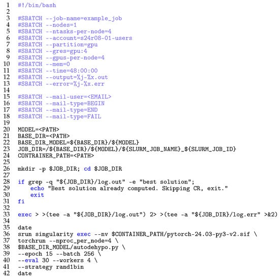
Figure 3. SBATCH script for job submission.

Furthermore, the workflow is used for training, evaluation, metrics, the storage of data in the appropriate data frame, and graph plotting based on newly acquired data, as presented in Figure 4. Finally, the dataset is loaded, and the basic steps of DE presented in Figure 1 are performed to evaluate and return the most suitable parameters for the training and evaluation phase. When the job is completed, we evaluate the performance metrics, which are saved in a data frame along with visualizations. Thus, we wanted to check the adequacy of the optimization of the hyperparameter space; i.e., we examined the number of epochs and iterations, weights, learning rate (LR), batch size, and optimizers. Given that it has been implemented and deployed, the AutoDEHypO workflow leverages the potential of utilizing multiple GPUs to run DE fitness functions for ML, as presented in Figure 4. In the evaluation phase, basic ML metrics were used (Section 2.1). To obtain, measure, and compare the utilization of computer resources of individual jobs, such as the elapsed time and energy consumption, data from Slurm were used [13].

Figure 4. Schematic overview of the analytics of the potential efficiency for the AutoDEHypO workflow.

3.5. Checkpoint and Restart, Collected Logs, and Fault Tolerance

Logging of the standard output and standard error output is enabled and generated in the event of an error. Email notifications are also set up to provide information on if a job is queued, started, completed, or failed [13]. This is important for certain cases where anomalies occur during initialization, such as when jobs need to be handled separately. The output files can be taken into account within the AutoDEHypO runtime, which can detect failures in settings, such as issues with NCCL or undetected GPUs within the initialization phase. One can look at these detections, from setting failures to the fact that CR uses feedback mechanisms to check which runs may need to be restarted (Figure 3 line 27). Furthermore, at the beginning of this experiment, we did not know how many resources were needed, and with the CR mechanism, we could accordingly adjust the input Slurm parameters and the need for the computational resource requirements, such as the job state, consumed energy, memory allocation, number of nodes, number of cores, number of cores per node, number of cores per CPU, number of tasks, number of GPUs, number of GPUs per node, and others. The Slurm command requeue allows the resubmission of a failed job when we can avoid and exclude any problematic nodes or, in the opposite case, when we do not want the submission, and a manual check is required after a certain number of—for example, 2—unsuccessful restarts; then, we can use the opposite command: no-requeue. This allows us to detect such errors in certain cases and perform an automatic restart of the job. Manual intervention is still required for cross-checking, and, if necessary, the job is resubmitted to the cluster queue, as shown in Figure 4. Due to the limitations of the experiment, the elapsed time and utilization of computer resources also needed to be taken into account.

4. Experimental Results

The experiments are divided into two phases of benchmarking. Within the first phase, we examine the efficiency of ML models and their parameters. The latter is then used in the second phase as a continuation of the experiments, to which we apply an analysis of the DE mutation strategies presented in Equations (8)–(12). The experiment had to be limited due to resource constraints such as time and the quota of computation resources granted within the development project on the largest Slovenian supercomputer, EuroHPC Vega. The ML models ResNet18, VGG11, ConvNeXtSmall, and DenseNet121 were used with public datasets. For the datasets, we chose CIFAR10 and CIFAR100, as they contain smaller images, thus providing a smaller size than other datasets, allowing them to be included, preprocessed, and trained [27]. The energy consumption is presented in Mega Joules (MJ) [13]. In order to obtain an assessment of the performance of the ML models and algorithms, aggregated statistics were calculated for the obtained results.

Taking into account that resource allocation may impact the obtained results, we ensured that all submitted job scripts had the same resource allocation [2]. Although it would have been possible to restrict our runs to a specific node using an additional Slurm option, this is not the intended use of HPC and was, hence, kept as a constraint. Therefore, jobs and runs were freely distributed across different nodes. During the initiation and execution of the experiment, we faced a few challenges on the software level that we could not avoid encountering, such as the wall time, which was set within the startup script, being too short, as well as a few others. The experiment was also run on the NVIDIA drivers and the Compute Unified Device Architecture (CUDA) Toolkit, which were updated at the beginning of the experiment, as we encountered a set of GPU nodes with incorrect configurations, which were resolved immediately, as well as hardware failures. This necessitated the replacement of DIMM modules and network cards, as well as the cleaning and resetting of network cards, GPUs, and other devices. Hardware problems in which GPUs are not available or are undetected lead to a failure of a large set of submitted jobs in less than 30 s on critical nodes due to failed internal communication through the NCCL back-end. In the event of such an error, a standard error output was generated, and an email notification was successfully received. Furthermore, the deployed CR was included as a common checkpoint for the ML model, therefore demonstrating how we saved important time with AutoDEHypO, with which we enabled resubmission. We received data on failed jobs, such as the time stamp, job state, job name, and job ID, that needed to be resubmitted. An example of the standard error output in the event of a runtime error is given in the following.

• RuntimeError:
• ProcessGroupNCCL is only supported with GPUs, no GPUs found!

The results obtained from the ResNet18, VGG11, ConvNeXtSmall, and DenseNet121 ML models on the CIFAR10 dataset are listed in Table 2, Table 3, Table 4 and Table 5, respectively. These tables present the batch size used and the results obtained, including the maximum achieved accuracy on the test batch, the best learning rate found, the best accuracy achieved, the CPU time consumed, the elapsed time, and the energy consumed in a Slurm job. Figure 5 provides an example of a subset for the ML performance of the ResNet18, VGG11, ConvNeXtSmall, and DenseNet121 ML models on the CIFAR10 dataset, and Figure 6 does so for the CIFAR100 dataset.

Table 2. Results obtained in 15 epochs using the ResNet18 ML model on CIFAR10.

Batch Size	Max Accuracy %	Best LR	Best Accuracy	Consumed CPU Time	Elapsed Time	Consumed Energy
16	95.394%	0.0006082014966333853	0.19592	1 d 02:55:36	06:43:54	8.26 MJ
32	96.008%	0.0007901080473489402	0.19534	1 d 01:54:56	06:28:44	7.94 MJ
64	96.296%	0.000738124409536461	0.1967	14:50:00	03:42:30	4.52 MJ
128	96.042%	0.00034871425456294697	0.19574	15:23:32	03:50:53	4.73 MJ
256	97.988%	0.0002672795926582179	0.19684	14:07:44	03:31:56	4.33 MJ

Table 3. Results obtained in 15 epochs using the VGG11 ML model on CIFAR10.

Batch Size	Max Accuracy %	Best LR	Best Accuracy	Consumed CPU Time	Elapsed Time	Consumed Energy
16	97.396%	0.00012525167316710355	0.19706	2 d 00:09:16	12:02:19	19.80 MJ
32	97.182%	0.000268894951638127	0.19714	1 d 03:35:24	06:53:51	11.03 MJ
64	97.408%	0.00024077230180039115	0.19774	19:02:36	04:45:39	7.37 MJ
128	97.686%	0.00019428618959243084	0.19824	15:15:12	03:48:48	5.46 MJ
256	97.584%	0.00034871425456294697	0.19758	18:09:48	04:32:27	6.40 MJ

Table 4. Results obtained in 15 epochs using the ConvNeXtSmall ML model on CIFAR10.

Batch Size	Max Accuracy %	Best LR	Best Accuracy	Consumed CPU Time	Elapsed Time	Consumed Energy
16	98.056%	0.00012034845529446537	0.1972	4 d 21:06:56	1 d 05:16:44	37.61 MJ
32	97.982%	0.00014014894006367788	0.19806	3 d 08:00:08	20:00:02	25.60 MJ
64	98.486%	0.0008678928687917702	0.19836	1 d 05:25:36	07:21:24	9.73 MJ
128	98.574%	0.00028135858111119703	0.19768	23:18:44	05:49:41	8.01 MJ
256	99.17%	0.0005148738101840251	0.19916	20:23:24	05:05:51	7.05 MJ

Table 5. Results obtained in 15 epochs using the DenseNet121 ML model on CIFAR10.

Batch Size	Max Accuracy %	Best LR	Best Accuracy	Consumed CPU Time	Elapsed Time	Consumed Energy
16	95.03%	0.0007912646326431301	0.1935	8 d 00:01:08	2 d 00:00:17	57.02 MJ
32	95.058%	0.0007901080473489402	0.19546	3 d 12:20:16	21:05:04	27.31 MJ
64	95.04%	0.0004894533183428303	0.19512	1 d 23:24:56	11:51:14	15.34 MJ
128	95.208%	0.00034871425456294697	0.19582	1 d 01:45:24	06:26:21	8.89 MJ
256	94.8%	0.0007901080473489402	0.19542	19:09:12	04:47:18	6.43 MJ

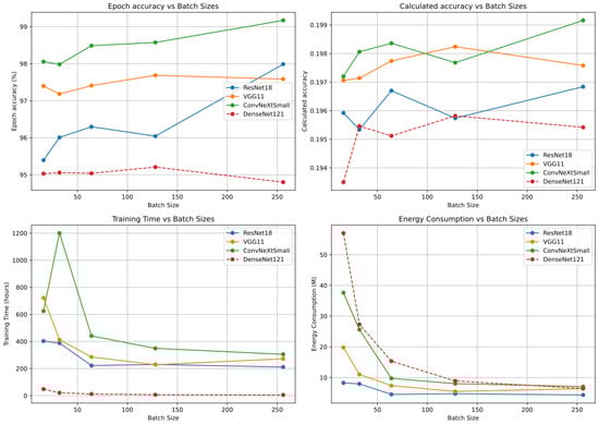
Figure 5. Plots of the initially obtained results of the ML metrics on the CIFAR10 dataset.

Figure 6. Plots of the initially obtained results of the ML metrics on the CIFAR100 dataset.

The results obtained from the ML models on the CIFAR100 dataset in the first initial phase are presented in Table 6 for ResNet18, for VGG11 in Table 7, for ConvNeXtSmall in Table 8, and for DenseNet121 in Table 9, respectively.

Table 6. Results obtained in 15 epochs using the ResNet18 ML model on CIFAR100.

Batch Size	Max Accuracy %	Best LR	Best Accuracy	Consumed CPU Time	Elapsed Time	Consumed Energy
16	79.978%	0.00044856335954386015	0.1838	1 d 21:46:52	11:26:43	14.57 MJ
32	86.23%	0.0008717460916603777	0.1844	22:44:28	05:41:07	7.08 MJ
64	87.168%	0.0005391893838907642	0.187	19:26:24	04:51:36	5.93 MJ
128	85.288%	0.0006082014966333853	0.1896	15:32:36	03:53:09	4.77 MJ
256	83.758%	0.0002422874901653207	0.1896	14:34:28	03:38:37	4.43 MJ

Table 7. Results obtained in 15 epochs using the VGG11 ML model on CIFAR100.

Batch Size	Max Accuracy %	Best LR	Best Accuracy	Consumed CPU Time	Elapsed Time	Consumed Energy
16	83.336%	0.00012525167316710355	0.1828	1 d 21:07:48	11:16:57	18.52 MJ
32	82.176%	0.0002092511621805628	0.1874	1 d 00:45:48	06:11:27	10.45 MJ
64	81.9%	0.00012525167316710355	0.1882	15:41:00	03:55:15	5.98 MJ
128	76.106%	0.00013244795866876926	0.1822	21:25:28	05:21:22	7.60 MJ
256	62.56%	0.00028135858111119703	0.1724	15:04:16	03:46:04	5.22 MJ

Table 8. Results obtained in 15 epochs using the ConvNeXtSmall ML model on CIFAR100.

Batch Size	Max Accuracy %	Best LR	Best Accuracy	Consumed CPU Time	Elapsed Time	Consumed Energy
16	97.086%	0.0003784156928188382	0.1988	5 d 23:48:48	1 d 11:57:12	45.13 MJ
32	97.494%	0.00012525167316710355	0.1984	1 d 03:46:48	06:56:42	8.86 MJ
64	97.954%	0.00023894652307312613	0.198	1 d 23:54:16	11:58:34	15.65 MJ
128	98.342%	0.00016177690430439908	0.1992	1 d 07:00:08	07:45:02	10.65 MJ
256	98.784%	0.00028135858111119703	0.199	15:59:36	03:59:54	5.97 MJ

Table 9. Results obtained in 15 epochs using the DenseNet121 ML model on CIFAR100.

Batch Size	Max Accuracy %	Best LR	Best Accuracy	Consumed CPU Time	Elapsed Time	Consumed Energy
16	78.902%	0.0007912646326431301	0.187	7 d 23:11:16	1 d 23:47:49	59.36 MJ
32	83.004%	0.0005677173263227356	0.1854	3 d 17:02:56	22:15:44	26.45 MJ
64	82.758%	0.0004164429342733091	0.1864	2 d 03:18:28	12:49:37	15.97 MJ
128	83.272%	0.0006600828705211815	0.1814	1 d 09:56:52	08:29:13	11.57 MJ
256	79.366%	0.0004894533183428303	0.181	20:16:40	05:04:10	7.05 MJ

4.1. Obtained Results

Based on the reported data provided and using our methodology, we observed results in Table 2, Table 3, Table 4 and Table 5 for CIFAR10 and in Table 6, Table 7, Table 8 and Table 9. These tables show a minimum achieved accuracy on test trial and their corresponding impact, highlighting their significance, where the lowest observed accuracy is 62.56%, which corresponds to the calculated ML accuracy of 0.1724. The highest achieved accuracy is 99.17%, with the calculated ML accuracy of 0.19916. Furthermore, for consumed energy metric, we obtained a minimum reported value of 4.43 M (ResNet18) and a maximum value of 59.36 M (DenseNet121). We also observed the elapsed time metric, ranging from the fastest completed job of 03:38:37, to the longest job with wall time 2 d 00:00:17 that exceeded the maximum allowed job execution time within the submitted partition. The results obtained in the first phase of the experiment possibly indicated that using a batch size of 256 in a set of ML models produced the most suitable and efficient results.

We observed that the DenseNet121 model possibly consumed more energy on both datasets than the less complex ML models, such as ResNet18, as presented in Figure 5 and Figure 6. Individual ML models in combination with certain DE strategies possibly performed better and more consistently, while some possibly consumed more energy, e.g., with the exponential DE strategies applied to DenseNet121 or ResNet18, and vice versa, with binomial models possibly consuming more resources in ConvNeXSmall and VGG11. The second phase of the experiment proceeded with a performance comparison of the binomial and exponential DE strategies with each ML model. In this phase, 10 independent runs were executed, as this could more generally determine whether there were significant differences DE-strategy-wise or ML-model-wise, and confirm if there was an impact on key metrics. A mutation was applied randomly with a factor (F) presented in Table 1. The population size (P) and the maximum possible number of generations (G) were appropriately determined due to the project allocation and resource constraints, otherwise we would exceed the current allowable resource consumption within the project allocation. The convergences of metric of accuracy is plotted unified through runtimes in Figure 7 for those runs that obtained median accuracy among each of the 10 independent runs of a DE strategy for a ML model. As observed, the effects of the DE strategies DE/rand/1/bin, DE/best/1/bin, DE/current-to-best/1/bin, DE/rand/2/bin, DE/best/2/bin, as well as the exponential strategies, such as DE/rand/1/exp, DE/best/1/exp, DE/current-to-best/1/exp, DE/rand/2/exp, and DE/best/2/exp [55], possibly varies across different ML model architectures, such as ResNet18, VGG11, ConvNeXtSmall, and DenseNet121, and the CIFAR10 and CIFAR100 datasets [27]. As the results of the tables indicate, $H_0$ is rejected because at least one DE strategy shows a significant difference, and specific DE strategies may even perform better. Therefore, to analyse which and for how much overall when aggregated, we discuss in the next subsection.

Figure 7. Accuracy convergences through runtime, for the median runs according to accuracy metric.

Figure 8 shows the statistical measure of the mean for each metric in the initial phase, and it is divided into three subplots (a) elapsed time, (b) consumed energy, and (c) accuracy for the DE strategies; these values were measured in 10 runs on the CIFAR10 dataset and are grouped by ML model. Figure 9 shows the same means of the selected DE strategies measured on the CIFAR100 dataset. Moreover, if we have a well-tuned ML model with appropriate weights, and the hyperparameters are poorly tuned, we possibly achieve worse ML performance over key metrics. Furthermore, the results obtained from the ResNet18, VGG11, ConvNeXtSmall, and DenseNet121 ML models with a batch size of 256 on both datasets show that, possibly, more efficient DE strategies consumed fewer resources, as the longer execution time possibly resulted in an increase the consumption of resources, and vice versa. A shorter execution time possibly resulted in lower resource consumption. The results on the CIFAR10 dataset are presented in Table A1, Table A2, Table A3 and Table A4, while the results on the CIFAR100 dataset are presented in Table A5, Table A6, Table A7 and Table A8.

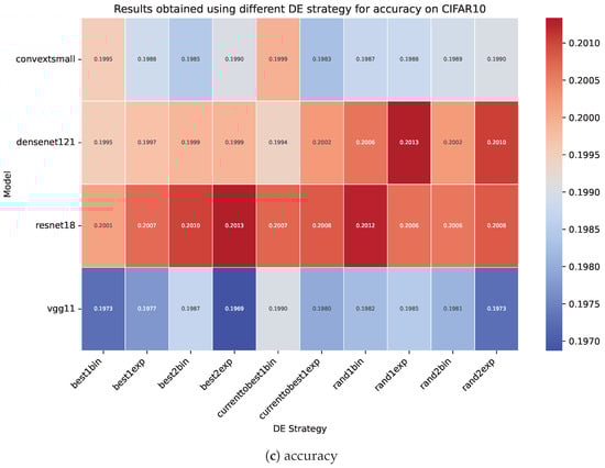
Figure 8. The statistical measures of the mean for the elapsed time (a), consumed energy (b), and accuracy (c) from the results obtained from 10 runs of 15 epochs of ML models that were hyperoptimized using the different DE strategies presented in Table A1, Table A2, Table A3 and Table A4. The x-axis represents the evaluated DE strategies, while the y-axis shows the ML models used.

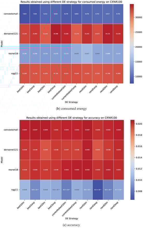
Figure 9. The statistical measures of the mean for the elapsed time (a), consumed energy (b), and accuracy (c) from the results obtained from 10 runs of 15 epochs of ML models that were hyperoptimized using the different DE strategies presented in Table A5, Table A6, Table A7 and Table A8. The x-axis represents the evaluated DE strategies, while the y-axis shows the ML models used.

4.2. Discussion of the Aggregated Statistics

Aggregate statistical analysis using non-parametric Friedman tests and corresponding procedures for the computational results of the DE strategies was performed on the ResNet18, VGG11, ConvNeXtSmall, and DenseNet121 ML models and on the CIFAR10 and CIFAR100 datasets [27,115]. Control tests were performed on the metrics of elapsed time, consumed energy, and accuracy using custom extraction scripts and publicly available code for statistics [116]. The p-value threshold was set to 0.05, and significant differences were detected and marked (†). This analysis was conducted to determine whether the DE strategies, ML models, and their architectures or a combination thereof had a statistically significant impact and if there were significant differences in key metrics for the computational efficiency. The results of the statistical analysis are presented in Table 10, Table 11, Table 12, Table 13, Table 14, Table 15, Table 16, Table 17 and Table 18.

Table 10. Statistical analysis of elapsed time in the DE strategies using a non-parametric Friedman test with the maximum rank distribution and corresponding post hoc procedures (rejected, as marked in bold and with ^† sign, at a statistical value below the threshold of 0.005555555555555556 for Bonferroni–Dunn, 0.05 for Holm and Hommel, 0.025 for Hochberg and Rom, 0.050000000000000044 for Holland and Finner, and 2.9216395384872545 × 10⁻¹⁷ for Li, respectively).

i	DE Strategy	$\mathit{z}=({\mathit{R}}_0-{\mathit{R}}_{\mathit{i}})/\mathit{SE}$	p	Holm/Hochberg/Hommel	Holland	Rom	Finner	Li
9	best1bin	5.32	1.05 × 10−7	0.00556 †	0.00568 †	0.00584 †	0.00568 †	2.92 × 10−17 †
8	best1exp	5.32	1.05 × 10−7	0.00625 †	0.00639 †	0.00657 †	0.0113 †	2.92 × 10−17 †
7	currenttobest1bin	3.91	9.07 × 10−5	0.00714 †	0.0073 †	0.00751 †	0.017 †	2.92 × 10−17 †
6	currenttobest1exp	2.92	0.00353	0.00833 †	0.00851 †	0.00876 †	0.0225 †	2.92 × 10−17 †
5	best2exp	2.62	0.00875	0.01 †	0.0102 †	0.0105 †	0.0281 †	2.92 × 10−17 †
4	best2bin	2.51	0.012	0.0125 †	0.0127 †	0.0131 †	0.0336 †	2.92 × 10−17 †
3	rand1bin	2.44	0.0148	0.0167 †	0.017 †	0.0167 †	0.0391 †	2.92 × 10−17 †
2	rand1exp	2.29	0.0221	0.025 †	0.0253 †	0.025 †	0.0446 †	2.92 × 10−17 †
1	rand2bin	6.56 × 10−16	1	0.05 †	0.05 †	0.05 †	0.05 †	0.05

Table 11. Statistical analysis of energy consumed in the DE strategies using the non-parametric Friedman test with the minimum rank distribution and corresponding post hoc procedures (rejected, as marked in bold and with ^† sign, at a statistical value below the threshold at 0.005555555555555556 for Bonferroni–Dunn, 0.016666666666666666 for Holm and Hommel, 0.0125 for Hochberg, 0.016952427508441503 for Holland, 0.013109375000000001 for Rom, 0.044570249746389234 for Finner, and 0.011483473500591115 for Li, respectively).

i	DE Strategy	$\mathit{z}=({\mathit{R}}_0-{\mathit{R}}_{\mathit{i}})/\mathit{SE}$	p	Holm/Hochberg/Hommel	Holland	Rom	Finner	Li
9	rand2bin	5.11	3.15 × 10−7 †	0.00556 †	0.00568 †	0.00584 †	0.00568 †	0.0115 †
8	rand2exp	4.99	6.19 × 10−7 †	0.00625 †	0.00639 †	0.00657 †	0.0113 †	0.0115 †
7	best2bin	2.73	0.00628 †	0.00714 †	0.0073 †	0.00751 †	0.017 †	0.0115 †
6	rand1bin	2.73	0.00628 †	0.00833 †	0.00851 †	0.00876 †	0.0225	0.0115 †
5	best2exp	2.58	0.00974 †	0.01 †	0.0102 †	0.0105 †	0.0281	0.0115 †
4	rand1exp	2.55	0.0108 †	0.0125 †	0.0127 †	0.0131 †	0.0336	0.0115 †
3	currenttobest1exp	2.14	0.0322	0.0167 †	0.017 †	0.0167 †	0.0391	0.0115 †
2	currenttobest1bin	0.702	0.483	0.025	0.0253	0.025	0.0446	0.0115 †
1	best1exp	0.277	0.782	0.05	0.05	0.05	0.05	0.05

Table 12. Statistical analysis of the accuracy in the DE strategies using the non-parametric Friedman test with the minimum rank distribution and corresponding post hoc procedures (rejected, as marked in bold and with ^† sign, at a statistical value below the threshold at 0.005555555555555556 for Bonferroni–Dunn, Holm, and Hommel, 0.005683044988048058 for Holland and Finner, and 7.7532015972022 ×10⁻⁴ for Li, respectively).

i	DE Strategy	$\mathit{z}=({\mathit{R}}_0-{\mathit{R}}_{\mathit{i}})/\mathit{SE}$	p	Holm/Hochberg/Hommel	Holland	Rom	Finner	Li
9	rand1exp	1.85	0.0648	0.00556 †	0.00568 †	0.00584	0.00568 †	0.000775
8	rand2bin	1.5	0.135	0.00625	0.00639	0.00657	0.0113	0.000775
7	rand1bin	1.44	0.15	0.00714	0.0073	0.00751	0.017	0.000775
6	currenttobest1bin	1.29	0.196	0.00833	0.00851	0.00876	0.0225	0.000775
5	rand2exp	0.96	0.337	0.01	0.0102	0.0105	0.0281	0.000775
4	best2bin	0.535	0.592	0.0125	0.0127	0.0131	0.0336	0.000775
3	currenttobest1exp	0.48	0.631	0.0167	0.017	0.0167	0.0391	0.000775
2	best1bin	0.24	0.81	0.025	0.0253	0.025	0.0446	0.000775
1	best2exp	0.0185	0.985	0.05	0.05	0.05	0.05	0.05

Table 13. Statistical analysis of the elapsed time in the DE strategies using the non-parametric Friedman test with the maximum rank distribution and corresponding post hoc procedures (rejected, as marked in bold and with ^† sign, at a statistical value below the threshold of 0.005555555555555556 for Bonferroni–Dunn, Holm, and Hommel, 0.005683044988048058 for Holland and Finner, and 0.015161939437253264 for Li, respectively).

i	DE Strategy	$\mathit{z}=({\mathit{R}}_0-{\mathit{R}}_{\mathit{i}})/\mathit{SE}$	p	Holm/Hochberg/Hommel	Holland	Rom	Finner	Li
9	best1exp	2.22	0.0267	0.00556 †	0.00568 †	0.00584	0.00568 †	0.0151 †
8	best2bin	2.18	0.0294	0.00625	0.00639	0.00657	0.0113	0.0151 †
7	best1bin	2.1	0.0353	0.00714	0.0073	0.00751	0.017	0.0151 †
6	currenttobest1bin	1.55	0.121	0.00833	0.00851	0.00876	0.0225	0.0151 †
5	currenttobest1exp	1.03	0.301	0.01	0.0102	0.0105	0.0281	0.0151 †
4	rand1bin	0.443	0.658	0.0125	0.0127	0.0131	0.0336	0.0151 †
3	rand1exp	0.406	0.685	0.0167	0.017	0.0167	0.0391	0.0151 †
2	best2exp	0.406	0.685	0.025	0.0253	0.025	0.0446	0.0151 †
1	rand2exp	0.369	0.712	0.05	0.05	0.05	0.05	0.05

Table 14. Statistical analysis of the energy consumed in the DE strategies using the non-parametric Friedman test with the minimum rank distribution and corresponding post hoc procedures (rejected, as marked in bold and with ^† sign, at a statistical value below the threshold of 0.005555555555555556 for Bonferroni–Dunn, Holm, and Hommel, 0.005683044988048058 for Holland and Finner, and 0.014435245666076669 for Li, respectively).

i	DE Strategy	$\mathit{z}=({\mathit{R}}_0-{\mathit{R}}_{\mathit{i}})/\mathit{SE}$	p	Holm/Hochberg/Hommel	Holland	Rom	Finner	Li
9	rand2bin	2.07	0.0386	0.00556 †	0.00568 †	0.00584	0.00568 †	0.0144 †
8	rand1bin	1.98	0.0482	0.00625	0.00639	0.00657	0.0113	0.0144 †
7	rand2exp	1.79	0.0733	0.00714	0.0073	0.00751	0.017	0.0144 †
6	best2exp	1.44	0.15	0.00833	0.00851	0.00876	0.0225	0.0144 †
5	currenttobest1exp	0.979	0.328	0.01	0.0102	0.0105	0.0281	0.0144 †
4	rand1exp	0.812	0.417	0.0125	0.0127	0.0131	0.0336	0.0144 †
3	currenttobest1bin	0.683	0.495	0.0167	0.017	0.0167	0.0391	0.0144 †
2	best2bin	0.425	0.671	0.025	0.0253	0.025	0.0446	0.0144 †
1	best1exp	0.351	0.726	0.05	0.05	0.05	0.05	0.05

Table 15. Statistical analysis of the accuracy in the DE strategies using the non-parametric Friedman test with the minimum rank distribution and corresponding post hoc procedures (rejected, as marked in bold and with ^† sign, at a statistical value below the threshold of 0.005555555555555556 for Bonferroni–Dunn and Hochberg, 0.00625 for Holm and Hommel, 0.006391150954545011 for Holland, 0.005843911024153359 for Rom, 0.011333792975759982 for Finner, and 0.03180542233195395 for Li, respectively).

i	DE Strategy	$\mathit{z}=({\mathit{R}}_0-{\mathit{R}}_{\mathit{i}})/\mathit{SE}$	p	Holm/Hochberg/Hommel	Holland	Rom	Finner	Li
9	rand1bin	2.81	0.00501 †	0.00556 †	0.00568 †	0.00584 †	0.00568 †	0.0318 †
8	rand2exp	2.23	0.0255	0.00625 †	0.00639 †	0.00657	0.0113	0.0318 †
7	currenttobest1exp	2.2	0.028	0.00714	0.0073	0.00751	0.017	0.0318 †
6	currenttobest1bin	1.96	0.0503	0.00833	0.00851	0.00876	0.0225	0.0318 †
5	rand2bin	1.46	0.145	0.01	0.0102	0.0105	0.0281	0.0318 †
4	best1bin	1.29	0.196	0.0125	0.0127	0.0131	0.0336	0.0318 †
3	best2exp	1.27	0.203	0.0167	0.017	0.0167	0.0391	0.0318 †
2	best1exp	1.26	0.209	0.025	0.0253	0.025	0.0446	0.0318 †
1	best2bin	0.849	0.396	0.05	0.05	0.05	0.05	0.05

Table 16. Statistical analysis of the elapsed time in the DE strategies using the non-parametric Friedman test with the maximum rank distribution and corresponding post hoc procedures (rejected, as marked in bold and with ^† sign, at a statistical value below the threshold of 0.005555555555555556 for Bonferroni–Dunn, 0.0125 for Holm and Hommel, 0.01 for Hochberg, 0.012741455098566168 for Holland, 0.010515350115740741 for Rom, 0.039109465610866256 for Finner, and 0.010841964200380961 for Li, respectively).

i	DE Strategy	$\mathit{z}=({\mathit{R}}_0-{\mathit{R}}_{\mathit{i}})/\mathit{SE}$	p	Holm/Hochberg/Hommel	Holland	Rom	Finner	Li
9	best1exp	5.33	1 × 10−7	0.00556 †	0.00568 †	0.00584 †	0.00568 †	0.0108 †
8	best1bin	5.25	1.53 × 10−7	0.00625 †	0.00639 †	0.00657 †	0.0113 †	0.0108 †
7	currenttobest1bin	3.86	0.000111	0.00714 †	0.0073 †	0.00751 †	0.017	0.0108 †
6	best2bin	3.32	0.000913	0.00833 †	0.00851 †	0.00876 †	0.0225	0.0108 †
5	currenttobest1exp	2.79	0.00521	0.01 †	0.0102 †	0.0105 †	0.0281	0.0108 †
4	best2exp	2.14	0.0323	0.0125 †	0.0127 †	0.0131	0.0336	0.0108 †
3	rand1bin	2.04	0.0417	0.0167	0.017	0.0167	0.0391	0.0108 †
2	rand1exp	1.91	0.0566	0.025	0.0253	0.025	0.0446	0.0108 †
1	rand2exp	0.261	0.794	0.05	0.05	0.05	0.05	0.05

Table 17. Statistical analysis of the energy consumed in the DE strategies using the non-parametric Friedman test with the maximum rank distribution and corresponding post hoc procedures (rejected, as marked in bold and with ^† sign, at a statistical value below the threshold of 0.005555555555555556 for Bonferroni–Dunn, 0.0125 for Hochberg, 0.016666666666666666 for Holm and Hommel, 0.016952427508441503 for Holland, 0.013109375000000001 for Rom, 0.044570249746389234 for Finner, and 0.011898018581242242 for Li, respectively).

i	DE Strategy	$\mathit{z}=({\mathit{R}}_0-{\mathit{R}}_{\mathit{i}})/\mathit{SE}$	p	Holm/Hochberg/Hommel	Holland	Rom	Finner	Li
9	best1bin	5.08	3.8 × 10−7	0.00556 †	0.00568 †	0.00584 †	0.00568 †	0.01189 †
8	best1exp	4.63	3.57 × 10−6	0.00625 †	0.00639 †	0.00657 †	0.0113 †	0.01189 †
7	currenttobest1bin	4.1	4.14 × 100	0.00714 †	0.0073 †	0.00751 †	0.017 †	0.01189 †
6	currenttobest1exp	2.87	0.00408	0.00833 †	0.00851 †	0.00876 †	0.0225	0.01189 †
5	best2bin	2.85	0.00442	0.01 †	0.0102 †	0.0105 †	0.0281	0.01189 †
4	rand1exp	2.7	0.00688	0.0125 †	0.0127 †	0.0131 †	0.0336	0.01189 †
3	best2exp	2.23	0.0256	0.0167 †	0.017 †	0.0167 †	0.0391	0.01189 †
2	rand1bin	1.75	0.0802	0.025	0.0253	0.025	0.0446	0.01189 †
1	rand2exp	0.287	0.774	0.05	0.05	0.05	0.05	0.05

Table 18. Statistical analysis of the accuracy in the DE strategies using the non-parametric Friedman test with the minimum rank distribution and corresponding post hoc procedures (rejected, as marked in bold and with ^† sign, at a statistical value below the threshold of 0.005555555555555556 for Bonferroni–Dunn, Holm and Hommel, 0.005683044988048058 for Holland, 0.005683044988048058 for Finner, and 0.0010964059917403937 for Li, respectively).

i	DE Strategy	$\mathit{z}=({\mathit{R}}_0-{\mathit{R}}_{\mathit{i}})/\mathit{SE}$	p	Holm/Hochberg/Hommel	Holland	Rom	Finner	Li
9	rand1bin	2.12	0.0344	0.00556 †	0.00568 †	0.00584	0.00568 †	0.00109 †
8	currenttobest1bin	1.41	0.159	0.00625	0.00639	0.00657	0.0113	0.00109 †
7	rand2exp	1.37	0.17	0.00714	0.0073	0.00751	0.017	0.00109 †
6	rand2bin	1.2	0.23	0.00833	0.00851	0.00876	0.0225	0.00109 †
5	currenttobest1exp	1.01	0.315	0.01	0.0102	0.0105	0.0281	0.00109 †
4	rand1exp	0.418	0.676	0.0125	0.0127	0.0131	0.0336	0.00109 †
3	best1bin	0.196	0.845	0.0167	0.017	0.0167	0.0391	0.00109 †
2	best2bin	0.0914	0.927	0.025	0.0253	0.025	0.0446	0.00109 †
1	best2exp	0.0261	0.979	0.05	0.05	0.05	0.05	0.05

Table 10 presents a statistical analysis of the elapsed time in the DE strategies using a non-parametric Friedman test, where the maximum rank highlights the advantage across the DE strategies, along with the corresponding post hoc procedures. The elapsed time in the DE strategies is significantly better than that of rand2exp on CIFAR10 when using AutoDEHypO according to the post hoc procedures of Holm, Hochberg, Hommel, Holland, and Finner. The Rom procedure shows a significant difference across DE strategies in comparison with rand2exp, with the exception of rand1exp. The Li procedure shows a significant difference across DE strategies in comparison with rand2exp, with the exception of rand2bin. Therefore, AutoDEHypO suggests that on CIFAR10, with the metric of elapsed time, the DE strategies best1bin, best1exp, currenttobest1bin, currenttobest1exp, best2exp, best2bin, rand1bin, rand1exp, and rand2bin are more suitable than rand2exp.

Table 11 presents a statistical analysis of the consumed energy in DE strategies using the non-parametric Friedman test, where the minimum rank highlights the advantage across DE strategies and corresponding post hoc procedures. The consumed energy in the DE strategies rand2bin, rand2exp, best2bin, rand1bin, best2exp, rand1exp, and currenttobest1exp is significantly better than in best1bin on CIFAR10 with AutoDEHypO according to the post hoc procedures of Holm, Hochberg, Hommel, Holland, and Rom. The Finner procedure shows that the DE strategies rand2bin, rand2exp, and best2bin are significantly better than rand2bin. Furthermore, rand1exp is significantly better than rand2bin according to the Holm, Hochberg, Hommel, and  Holland procedures. The Li procedure shows significant difference across DE strategies in comparison with best1bin, with the exception of best1exp. Therefore, AutoDEHypO suggests that on CIFAR10, for the metric of consumed energy, the DE strategies rand2bin, rand2exp, best2bin, rand1bin, best2exp, rand1exp, and currenttobest1exp are more suitable than currenttobest1bin, best1exp, and best1bin.

Table 12 presents a statistical analysis of the accuracy in the DE strategies using the non-parametric Friedman test, where the highest rank highlights the advantage across DE strategies and corresponding post hoc procedures. The accuracy in the DE strategy rand1exp is significantly better than that in best1exp on CIFAR10 with AutoDEHypO according to the post hoc procedures of Holm, Holland, and Finner. Therefore, AutoDEHypO suggests that on CIFAR10, for the metric of accuracy, the DE strategy rand1exp is more suitable than best1exp, rand2bin, rand1bin, currenttobest1bin, rand2exp, best2bin, currenttobest1exp, best1bin, and best2exp.

Table 13 presents a statistical analysis of the elapsed time in the DE strategies using the non-parametric Friedman test, where the maximum rank highlights the advantage across DE strategies and corresponding post hoc procedures. The elapsed time in the DE strategy best1exp is significantly better than that in rand2bin on CIFAR100 with AutoDEHypO according to the post hoc procedures of Holm, Holland, and Finner. The Li procedure shows significant differences across DE strategies in comparison with rand2bin, with the exception of rand2exp. Therefore, AutoDEHypO suggests that on CIFAR100, for the metric of elapsed time, the DE strategy best1exp is more suitable than rand2bin, best2bin, best1bin, currenttobest1bin, currenttobest1exp, rand1bin, rand1exp, best2exp, and rand2exp.

Table 14 presents a statistical analysis of the energy consumed in the DE strategies using the non-parametric Friedman test, where the minimum rank highlights the advantage across DE strategies and corresponding post hoc procedures. The energy consumed in the DE strategy rand2bin is significantly better than that in best1bin on CIFAR100 with AutoDEHypO according to the post hoc procedures of Holm, Hommel, Holland, and Finner. The Li procedure shows significant differences across DE strategies in comparison with best1bin, with the exception of best1exp. Therefore, AutoDEHypO suggests that on CIFAR100, for the metric of consumed energy, the DE strategy rand2bin is more suitable than best1bin, rand1bin, rand2exp, best2exp, currenttobest1exp, rand1exp, currenttobest1bin, best2bin, and best1exp.

Table 15 presents a statistical analysis of the accuracy in the DE strategies using the non-parametric Friedman test, where the highest rank highlights the advantage across DE strategies and corresponding post hoc procedures. The accuracy in the DE strategy rand1bin is significantly better than that in rand1exp on CIFAR100 with AutoDEHypO according to the post hoc procedures of Holm, Hommel, Holland, Rom and Finner. The DE strategy best2bin is significantly better than rand1exp according to the procedures of Holm, Hommel, and Holland. The Li procedure shows significant differences across DE strategies in comparison with rand1exp, with the exception of best2bin. Therefore, AutoDEHypO suggests that on CIFAR100, for the metric of accuracy, the DE strategies rand1bin and rand2exp are more suitable than rand1exp, currenttobest1exp, currenttobest1bin, rand2bin, best1bin, best2exp, best1exp, and best2bin.

Table 16 presents a statistical analysis of the elapsed time in the DE strategies using the non-parametric Friedman test, where the maximum rank highlights the advantage across DE strategies and corresponding post hoc procedures. The elapsed time in the DE strategies best1exp and best1bin is significantly better than that in rand2bin on CIFAR10 and CIFAR100 with AutoDEHypO according to the post hoc procedures of Holm, Hochberg, Holland, Rom, and Finner. Additionally, the DE strategies currenttobest1bin, best2bin, and currenttobest1exp are significantly better than rand2bin according to the procedures of Holm, Hochberg, Hommel, Holland, and Rom. best2exp is significantly better than rand2bin according to the procedures of Holm, Hochberg, Hommel, and Holland. The Li procedure shows significant differences across DE strategies in comparison with rand2bin, with the exception of rand2exp. Therefore, AutoDEHypO suggests that on CIFAR10 and CIFAR100, for the metric of elapsed time, the DE strategies best1exp, best1bin, currenttobest1bin, best2bin, currenttobest1exp, and best2exp are more suitable than rand1bin, rand1exp, and rand2exp.

Table 17 presents a statistical analysis of the energy consumed in the DE strategies using the non-parametric Friedman test, where the maximum rank highlights the advantage across DE strategies and corresponding post hoc procedures. The  energy consumed in the DE strategies best1bin, best1exp, currenttobest1bin, currenttobest1exp, best2bin, rand1exp, and best2exp is significantly better than that in rand2bin on CIFAR10 and CIFAR100 with AutoDEHypO according to the post hoc procedures of Holm, Hochberg, Hommel, Holland, and Rom. According to Finner’s post hoc procedure, the DE strategies best1bin, best1exp, and currenttobest1bin are significantly better than rand2bin. The Li procedure shows significant differences across DE strategies in comparison with rand2bin, with the exception of rand2exp. Therefore, AutoDEHypO suggests that on CIFAR10 and CIFAR100, for the metric of consumed energy, the DE strategies best1bin, best1exp, currenttobest1bin, currenttobest1exp, best2bin, rand1exp, and best2exp are more suitable than rand2bin, rand1bin, and rand2exp.

Table 18 presents a statistical analysis of the accuracy in the DE strategies using the non-parametric Friedman test, where the highest rank highlights the advantage across DE strategies and corresponding post hoc procedures. The accuracy in the DE strategy rand1bin is significantly better than that in best1exp on CIFAR10 and CIFAR100 with AutoDEHypO according to the post hoc procedures of Holm, Hommel, Holland, and Finner. The Li procedure shows significant differences across DE strategies in comparison with best1exp, with the exception of best2exp. Therefore, AutoDEHypO suggests that on CIFAR10 and CIFAR100, for the metric of accuracy, the DE strategy rand1bin is more suitable than best1exp, currenttobest1bin, rand2exp, rand2bin, currenttobest1exp, rand1exp, best1bin, best2bin, and best2exp.

As shown in Table 10, Table 11 and Table 12, according to Holm, Hochberg, Hommel, Holland, and Finner, on CIFAR10, several DE strategies perform significantly better than rand2exp, with additional confirmation from the Rom and Li procedures, except for rand2bin. The DE strategy best1exp runs significantly better than rand2bin, with confirmation from Li (with the exception of rand2exp). Furthermore, the energy consumption in the DE strategies rand2bin, rand2exp, best2bin, rand1bin, best2exp, rand1exp, and currenttobest1exp is significantly better than that in best1bin, with confirmation from Li, except for rand2exp. Table 16, Table 17 and Table 18 present results on both CIFAR10 and CIFAR100, where best1bin, best1exp, currenttobest1bin, currenttobest1exp, best2bin, rand1exp, and best2exp perform significantly better than rand2bin in terms of metrics according to the Li procedure, with exception of rand2exp. In terms of accuracy, best1exp outperforms rand1exp on CIFAR10. As shown in Table 13, Table 14 and Table 15, on CIFAR100, rand1bin achieves significantly better accuracy than that of rand1exp, with confirmation from Li, with the exception of best2bin. Across both datasets, rand1bin also demonstrates significantly better accuracy than that of best1exp, except for best2exp, according to the Li procedure.

Table 19 presents an overview of the outcomes of the statistical analysis and the aggregated number (counts) of confirmed out of 450, 184 (40.8%) significant differences in the DE strategies counting each post hoc procedure across the tree key metrics. These outcomes show and confirm significant differences in elapsed time, energy efficiency, and accuracy across the DE strategies. In addition to the elapsed time and accuracy, our operational data analytics also confirm the impact on energy efficiency when selecting DE strategies.

Table 19. Overview of the outcomes of the statistical analysis for the metrics of elapsed time, energy efficiency, and accuracy in the DE strategies using the non-parametric Friedman test on both the CIFAR10 and CIFAR00 datasets.

DE Strategy	Holm/Hochberg/Hommel	Holland	Rom	Finner	Li
best1bin	3	3	3	3	5
best2bin	4	4	4	2	8
best1exp	4	4	3	4	5
best2exp	4	4	4	1	6
currenttobest1bin	3	3	3	2	8
currenttobest1exp	4	4	4	1	8
rand1bin	4	4	4	3	8
rand2bin	3	3	2	3	2
rand1exp	4	4	3	2	7
rand2exp	2	2	1	1	4

As ML models depend on the input data characteristics and on the computational complexity of ML architecture designs, it is expected that some ML models are more suitable. To check this, we tested the suitability of some ML models by detecting differences in elapsed time, consumed energy, and accuracy. The aggregated test outcomes are seen in Table 20, where, for all three key metrics (elapsed time, consumed energy, and accuracy), it is evident from the Friedman rankings that the ResNet18 and ConvNextSmall ML models are ranked higher than the other two ML models, DenseNet121 and VGG11. These ranks are significantly different for the accuracy metric in the case of VGG11. For the metrics of elapsed time and consumed energy, in the case of VGG11, this is also significant. Moreover, significant differences from ML model DenseNet121 are also detected, i.e., these two (DenseNet121 and VGG11) require significantly more energy and time than ResNet18 and ConvNextSmall.

Table 20. Friedman rankings detected differences in elapsed time, consumed energy, and accuracy aggregated across ML models. The individual rankings demonstrate significant differences using the Holm/Hochberg/Hommel, Holland, Rom, Finner, and Li procedures, with a few exceptions for the post hoc procedures (the Rom and Li procedures for time and energy detect these differences only when comparing VGG11 and DenseNet121 against ResNet18 and ConvNextSmall, i.e., for 41 (91.1%) out of 45 rankings in the post hoc procedures, we successfully detected significant differences).

ML Model	Elapsed Time	Consumed Energy	Accuracy
resnet18	1.505000000000001	1.4800000000000006	1.394999999999994
convnextsmall	1.4949999999999906	1.5299999999999907	2.6374999999999935
densenet121	3.3250000000000006	3.2925000000000013	2.6725000000000008
vgg11	3.67500000000001	3.6975000000000096	3.295000000000002

Furthermore, significant differences between four ML models for 10 DE strategies (denoted as k) evaluations per each run result in 20 combinations (denoted as N), with critical value $q_{\alpha }$ of $2.394$ from the the two-tailed Bonferroni-Dunn test for k is studentized range statistic at the significance level $\alpha$ threshold of $0.05$ on their Friedman average ranks. To compare their ranks we calculated critical difference (CD) [117] of approximately $0.9773$. Additionally, we calculated confidence intervals (CI) based on CD, which detected significant difference in 11 (61.11%) out of 18 pairwise comparisons. The results are presented in Table 21.

Table 21. Ranks and confidence intervals for key metrics elapsed time, consumed energy, and accuracy across ML Models ResNet18, ConvNextSmall, DenseNet121, and VGG11 on CIFAR10 and CIFAR100 datasets.

ML Model Pair	Metric	Rank Difference	Confidence Interval (CI)	Significant
resnet18—convnextsmall	elapsed time	0.010000	[−0.967, 0.987]	No
resnet18—densenet121	elapsed time	−1.820000	[−2.797, −0.843]	Yes
resnet18—vgg11	elapsed time	−2.170000	[−3.147, −1.193]	Yes
convnextsmall—densenet121	elapsed time	−1.830000	[−2.807, −0.853]	Yes
convnextsmall—vgg11	elapsed time	−2.180000	[−3.157, −1.203]	Yes
densenet121—vgg11	elapsed time	−0.350000	[−1.327, 0.627]	No
resnet18—convnextsmall	consumed energy	−0.050000	[−1.027, 0.927]	No
resnet18—densenet121	consumed energy	−1.813000	[−2.79, −0.836]	Yes
resnet18—vgg11	consumed energy	−2.218000	[−3.195, −1.241]	Yes
convnextsmall—densenet121	consumed energy	−1.763000	[−2.74, −0.786]	Yes
convnextsmall—vgg11	consumed energy	−2.168000	[−3.145, −1.191]	Yes
densenet121—vgg11	consumed energy	−0.405000	[−1.382, 0.572]	No
resnet18—convnextsmall	accuracy	−1.242000	[−2.219, −0.265]	Yes
resnet18—densenet121	accuracy	−1.278000	[−2.255, −0.301]	Yes
resnet18—vgg11	accuracy	−1.900000	[−2.877, −0.923]	Yes
convnextsmall—densenet121	accuracy	−0.036000	[−1.013, 0.941]	No
convnextsmall—vgg11	accuracy	−0.658000	[−1.635, 0.319]	No
densenet121—vgg11	accuracy	−0.622000	[−1.599, 0.355]	No

5. Conclusions and Future Work

In this article, we presented the deployment of a high-performance differential-evolution-based hyperparameter optimization workflow (AutoDEHypO) for energy efficiency and operational data analytics on multiple GPUs, where a DE algorithm with different DE strategies is demonstrated and applied in hyperparameter optimization while considering key factors such as the ML model, dataset, and DE strategy. The challenge of the optimization of ML models in HPC environments was addressed by balancing the ML accuracy, energy consumption, and resource utilization. Practical limitations such as project time constraints and the computational resources allocated to this project on a part of the national share of HPC Vega may have influenced the experiment through aspects such as node availability, high cluster utilization, shared node scheduling, elapsed time and partition (wall time) limitations, network congestion, job failures, undetected GPUs, and limited granularity in energy measurement at the node level. The utilization of computing resources had to be carefully considered, and the evaluation metrics and their scope must be taken into account. AutoDEHypO detected significant differences in the utilization of HPC resources in terms of elapsed time, energy efficiency, and ML accuracy across DE strategies. Furthermore, AutoDEHypO overcomes several limitations of existing workflows, which mostly focus on ML performance, inefficient utilization of computational resources during job allocation, and extended queue times; therefore, there is a lack of integration with HPC environments and schedulers such as Slurm and limited support for sustainability and cost-effectiveness. In addition to tracking the elapsed time and accuracy, our AutoDEHypO uses operational data analytics to determine how energy efficiently DE algorithms and DE strategies perform and confirms the impact on energy efficiency when selecting DE strategies. The analytics of DE strategies influenced the consumption of resources and indicated when the consumption of energy and other resources led to different ML performance and configurations. Furthermore, the statistical analysis of the key metrics of elapsed time, consumed energy, and accuracy demonstrated significant differences in DE strategies and ML models by using the non-parametric Friedman test and corresponding post hoc procedures for CIFAR10 and CIFAR100 datasets.

Specifically, in 10 independent runs, the DE binomial mutation strategies were applied and out of 450 comparisons, 184 (40.8%) detected significant differences between strategies. The effect of used DE strategies DE/rand/1/bin, DE/best/1/bin, DE/current-to-best/1/bin, DE/rand/2/bin, DE/best/2/bin, and exponential such as DE/rand/1/exp, DE/best/1/exp, DE/current-to-best/1/exp, DE/rand/2/exp, and DE/best/2/exp varied across differentent ML model architectures such as ResNet18, VGG11, ConvNeXtSmall and DenseNet121, on datasets CIFAR10 and CIFAR100.

Additionally, as an important outcome, the ML model comparisons show that there are 41 (91.1%) out of 45 rankings in the post hoc procedures, where AutoDEHypO successfully detected significant differences in all three key metrics in the case of the VGG11 ML model; for the metrics of elapsed time and consumed energy, there were further significant differences detected in the DenseNet121 and VGG11 models when compared with the better ML models of ConvNextSmall and ResNet18. Furthermore, the calculated confidence intervals based on critical difference of approximately $0.9773$, detected significant differences in 11 (61.11%) out of 18 pairwise comparisons.

Despite the insights and contributions provided by this article, there are a few limitations to acknowledge. This workflow is designed and optimized for deployment on a single cluster. Generalizing this workflow to another HPC environment may be challenging due to differences in architecture, scheduling policies, and energy monitoring solutions. Furthermore, within the proposed workflow, we used a basic DE algorithm implementation and limited this research to a few ML models, two datasets (CIFAR10 and CIFAR100), a single DE algorithm, 10 DE strategies, and limited runs of each epoch. While this setup was sufficient for initial exploration and experimentation, further research can be conducted. Moreover, this workflow can be adopted for other ML models, such as neural networks with adjustments in their architectures, different DE algorithms and DE strategies, population sizes, and different datasets, such as ImageNet, MNIST, and others; last but not least, more computational resources can be used. Possibilities have emerged for the evaluation and validation of other algorithms and AutoML frameworks to provide a baseline comparison with state-of-the-art AutoML frameworks and beyond. The necessary validation and comparison for a different environment could take place within an additional experiment; this could include a comparison of the final results. System malfunctions may also be resolved through fault-tolerance mechanisms such as Checkpoint and Restart (CR) without affecting the obtained results, allowing one to continue after unexpected interruptions. Additionally, we can apply CR inside the DE loop, where we can continue from the last successfully saved and calculated generation. Furthermore, a real-time feedback mechanism for adaptive and dynamic changes within ML operations has not yet been implemented and may contribute to the workflow; this may be researched in the future. The prediction model and decision making based on historical data can contribute to ML performance, optimization, and energy efficiency. These improvements will not only strengthen the practical applicability of this workflow but also contribute to sustainability, and a reduction in the environmental footprint.

References

- Silva, C.; Vilaça, R.; Pereira, A.; Bessa, R. A review on the decarbonization of high-performance computing centers. Renew. Sustain. Energy Rev. 2024, 189, 114019. [Google Scholar] [CrossRef]
- Chu, X.; Hofstätter, D.; Ilager, S.; Talluri, S.; Kampert, D.; Podareanu, D.; Duplyakin, D.; Brandic, I.; Iosup, A. Generic and ML Workloads in an HPC Datacenter: Node Energy, Job Failures, and Node-Job Analysis. arXiv 2024, arXiv:2409.08949. [Google Scholar] [CrossRef]
- Baratchi, M.; Wang, C.; Limmer, S.; van Rijn, J.N.; Hoos, H.; Bäck, T.; Olhofer, M. Automated machine learning: Past, present and future. Artif. Intell. Rev. 2024, 57, 122. [Google Scholar] [CrossRef]
- Bolón-Canedo, V.; Morán-Fernández, L.; Cancela, B.; Alonso-Betanzos, A. A review of green artificial intelligence: Towards a more sustainable future. Neurocomputing 2024, 599, 128096. [Google Scholar] [CrossRef]
- TOP500 Methodology. 2025. Available online: https://www.top500.org/static/media/uploads/methodology-2.0rc1.pdf (accessed on 19 January 2025).
- Miller, J.; Trümper, L.; Terboven, C.; Müller, M.S. A Theoretical Model for Global Optimization of Parallel Algorithms. Mathematics 2021, 9, 1685. [Google Scholar] [CrossRef]
- Damme, P.; Birkenbach, M.; Bitsakos, C.; Boehm, M.; Bonnet, P.; Ciorba, F.; Dokter, M.; Dowgiallo, P.; Eleliemy, A.; Faerber, C.; et al. DAPHNE: An Open and Extensible System Infrastructure for Integrated Data Analysis Pipelines. In Proceedings of the Conference on Innovative Data Systems Research, Chaminade, CA, USA, 9–12 January 2022. [Google Scholar]
- Alangari, N.; El Bachir Menai, M.; Mathkour, H.; Almosallam, I. Exploring Evaluation Methods for Interpretable Machine Learning: A Survey. Information 2023, 14, 469. [Google Scholar] [CrossRef]
- Jakobsche, T.; Lachiche, N.; Ciorba, F.M. Investigating HPC Job Resource Requests and Job Efficiency Reporting. In Proceedings of the 2023 22nd International Symposium on Parallel and Distributed Computing (ISPDC), Bucharest, Romania, 10–12 July 2023; pp. 61–68. [Google Scholar] [CrossRef]
- Yarally, T.; Cruz, L.; Feitosa, D.; Sallou, J.; van Deursen, A. Uncovering Energy-Efficient Practices in Deep Learning Training: Preliminary Steps Towards Green AI. In Proceedings of the 2023 IEEE/ACM 2nd International Conference on AI Engineering—Software Engineering for AI (CAIN), Melbourne, Australia, 15–16 May 2023; pp. 25–36. [Google Scholar] [CrossRef]
- Prica, T. Development and supporting activities on EuroHPC Vega. In Proceedings of the Austrian-Slovenian HPC Meeting 2024—ASHPC24, Grundlsee, Austria, 10–13 June 2024; p. 14. [Google Scholar]
- Oliveira, S.d.; Topsakal, O.; Toker, O. Benchmarking Automated Machine Learning (AutoML) Frameworks for Object Detection. Information 2024, 15, 63. [Google Scholar] [CrossRef]
- Yoo, A.B.; Jette, M.A.; Grondona, M. SLURM: Simple Linux Utility for Resource Management. In Proceedings of the 9th International Workshop on Job Scheduling Strategies for Parallel Processing (JSSPP), Seattle, WA, USA, 24 June 2003. [Google Scholar] [CrossRef]
- Han, M.; Wu, H.; Chen, Z.; Li, M.; Zhang, X. A survey of multi-label classification based on supervised and semi-supervised learning. Int. J. Mach. Learn. Cybern. 2023, 14, 697–724. [Google Scholar] [CrossRef]
- Virtanen, P.; Gommers, R.; Oliphant, T.E.; Haberland, M.; Reddy, T.; Cournapeau, D.; Burovski, E.; Peterson, P.; Weckesser, W.; Bright, J.; et al. SciPy 1.0: Fundamental algorithms for scientific computing in Python. Nat. Methods 2020, 17, 261–272. [Google Scholar] [CrossRef]
- Das, S.; Mullick, S.S.; Suganthan, P.N. Recent Advances in Differential Evolution—An Updated Survey. Swarm Evol. Comput. 2016, 27, 1–30. [Google Scholar] [CrossRef]
- Li, J.Y.; Zhan, Z.H.; Zhang, J. Evolutionary Computation for Expensive Optimization: A Survey. Mach. Intell. Res. 2022, 19, 3–23. [Google Scholar] [CrossRef]
- Qin, X.; Luo, Y.; Chen, S.; Chen, Y.; Han, Y. Investigation of Energy-Saving Strategy for Parallel Variable Frequency Pump System Based on Improved Differential Evolution Algorithm. Energies 2022, 15, 5360. [Google Scholar] [CrossRef]
- Dragoi, E.N.; Dafinescu, V. Parameter control and hybridization techniques in differential evolution: A survey. Artif. Intell. Rev. 2015, 45, 447–470. [Google Scholar] [CrossRef]
- Storn, R.; Price, K. Differential Evolution–A Simple and Efficient Heuristic for global Optimization over Continuous Spaces. J. Glob. Optim. 1997, 11, 341–359. [Google Scholar] [CrossRef]
- Eltaeib, T.; Mahmood, A. Differential Evolution: A Survey and Analysis. Appl. Sci. 2018, 8, 1945. [Google Scholar] [CrossRef]
- Nanthapodej, R.; Liu, C.H.; Nitisiri, K.; Pattanapairoj, S. Hybrid Differential Evolution Algorithm and Adaptive Large Neighborhood Search to Solve Parallel Machine Scheduling to Minimize Energy Consumption in Consideration of Machine-Load Balance Problems. Sustainability 2021, 13, 5470. [Google Scholar] [CrossRef]
- Chhabra, A.; Sahana, S.K.; Sani, N.S.; Mohammadzadeh, A.; Omar, H.A. Energy-Aware Bag-of-Tasks Scheduling in the Cloud Computing System Using Hybrid Oppositional Differential Evolution-Enabled Whale Optimization Algorithm. Energies 2022, 15, 4571. [Google Scholar] [CrossRef]
- IAM Working Group. IPMI Specification. 2006. Available online: https://openipmi.sourceforge.io/IPMI.pdf (accessed on 25 October 2024).
- Bischl, B.; Binder, M.; Lang, M.; Pielok, T.; Richter, J.; Coors, S.; Thomas, J.; Ullmann, T.; Becker, M.; Boulesteix, A.L.; et al. Hyperparameter optimization: Foundations, algorithms, best practices, and open challenges. WIREs Data Min. Knowl. Discov. 2023, 13, e1484. [Google Scholar] [CrossRef]
- Morales-Hernández, A.; Van Nieuwenhuyse, I.; Rojas Gonzalez, S. A survey on multi-objective hyperparameter optimization algorithms for machine learning. Artif. Intell. Rev. 2022, 56, 8043–8093. [Google Scholar] [CrossRef]
- Dataset CIFAR10 and CIFAR100. Available online: https://www.cs.toronto.edu/~kriz/cifar.html (accessed on 19 November 2024).
- Boito, F.; Brandt, J.; Cardellini, V.; Carns, P.; Ciorba, F.M.; Egan, H. Autonomy Loops for Monitoring, Operational Data Analytics, Feedback, and Response in HPC Operations. In Proceedings of the 2023 IEEE International Conference on Cluster Computing Workshops (CLUSTER Workshops), Santa Fe, NM, USA, 31 October 2023; pp. 37–43. [Google Scholar] [CrossRef]
- El Naqa, I.; Murphy, M.J. What Is Machine Learning? In Machine Learning in Radiation Oncology: Theory and Applications; Springer International Publishing: Cham, Switzerland, 2015; pp. 3–11. [Google Scholar] [CrossRef]
- Zhang, X.; Guo, F.; Chen, T.; Pan, L.; Beliakov, G.; Wu, J. A Brief Survey of Machine Learning and Deep Learning Techniques for E-Commerce Research. J. Theor. Appl. Electron. Commer. Res. 2023, 18, 2188–2216. [Google Scholar] [CrossRef]
- Bergstra, J.; Bardenet, R.; Bengio, Y.; Kégl, B. Algorithms for hyper-parameter optimization. In Proceedings of the 25th International Conference on Neural Information Processing Systems, NIPS’11, Granada, Spain, 12–15 December 2011; Curran Associates Inc.: Red Hook, NY, USA, 2011; pp. 2546–2554. Available online: https://dl.acm.org/doi/10.5555/2986459.2986743 (accessed on 7 April 2025).
- Zamuda, A.; Daniel Hernández Sosa, J.; Adler, L. Improving constrained glider trajectories for ocean eddy border sampling within extended mission planning time. In Proceedings of the 2016 IEEE Congress on Evolutionary Computation (CEC), Vancouver, BC, Canada, 24–29 July 2016; pp. 1727–1734. [Google Scholar] [CrossRef]
- Zhu, K.; Wu, J. Residual attention: A simple but effective method for multi-label recognition. In Proceedings of the IEEE/CVF International Conference on Computer Vision, Montreal, QC, Canada, 10–17 October 2021; pp. 184–193. [Google Scholar] [CrossRef]
- Zhou, Z.H. Machine Learning; Springer Nature: Berlin/Heidelberg, Germany, 2021. [Google Scholar]
- Hu, X.; Chu, L.; Pei, J.; Liu, W.; Bian, J. Model Complexity of Deep Learning: A Survey. arXiv 2021, arXiv:2103.05127. [Google Scholar] [CrossRef]
- Radford, A.; Narasimhan, K.; Salimans, T.; Sutskever, I. Improving Language Understanding by Generative Pre-Training; OpenAI: San Francisco, CA, USA, 2018. [Google Scholar]
- Menik, S.; Ramaswamy, L. Towards Modular Machine Learning Solution Development: Benefits and Trade-offs. arXiv 2023, arXiv:2301.09753. [Google Scholar] [CrossRef]
- Shen, Y.; Zhang, Z.; Cao, T.; Tan, S.; Chen, Z.; Gan, C. ModuleFormer: Modularity Emerges from Mixture-of-Experts. arXiv 2023, arXiv:2306.04640. [Google Scholar] [CrossRef]
- Barandas, M.; Famiglini, L.; Campagner, A.; Folgado, D.; Simão, R.; Cabitza, F.; Gamboa, H. Evaluation of uncertainty quantification methods in multi-label classification: A case study with automatic diagnosis of electrocardiogram. Inf. Fusion 2024, 101, 101978. [Google Scholar] [CrossRef]
- Maloney, S.; Suarez, E.; Eicker, N.; Guimarães, F.; Frings, W. Analyzing HPC Monitoring Data With a View Towards Efficient Resource Utilization. In Proceedings of the 2024 IEEE 36th International Symposium on Computer Architecture and High Performance Computing (SBAC-PAD), Hilo, HI, USA, 13–15 November 2024; pp. 170–181. [Google Scholar]
- Vontzalidis, A.; Psomadakis, S.; Bitsakos, C.; Dokter, M.; Innerebner, K.; Damme, P.; Boehm, M.; Ciorba, F.; Eleliemy, A.; Karakostas, V.; et al. DAPHNE Runtime: Harnessing Parallelism for‚ Integrated Data Analysis Pipelines. In Proceedings of the Euro-Par 2023: Parallel Processing Workshops, Limassol, Cyprus, 28 August–1 September 2023; pp. 242–246. [Google Scholar]
- Jakobsche, T.; Lachiche, N.; Ciorba, F.M. Challenges and Opportunities of Machine Learning for Monitoring and Operational Data Analytics in Quantitative Codesign of Supercomputers. arXiv 2022, arXiv:2209.07164. [Google Scholar] [CrossRef]
- Prica, T.; Zamuda, A. Monitoring Energy Consumption of Workloads on HPC Vega. In Proceedings of the 6th ISC HPC International Workshop on “Monitoring & Operational Data Analytics”, Hamburg, Germany, 9 March–13 June 2025. [Google Scholar]
- Chakraborty, U.K. Advances in Differential Evolution; Springer Science & Business Media: Berlin/Heidelberg, Germany, 2008; Volume 143. [Google Scholar]
- Ahmad, M.F.; Isa, N.A.M.; Lim, W.H.; Ang, K.M. Differential evolution: A recent review based on state-of-the-art works. Alex. Eng. J. 2022, 61, 3831–3872. [Google Scholar] [CrossRef]
- Glotić, A.; Zamuda, A. Short-term combined economic and emission hydrothermal optimization by surrogate differential evolution. Appl. Energy 2015, 141, 42–56. [Google Scholar] [CrossRef]
- Zamuda, A.; Sosa, J.D.H.; Adler, L. Constrained differential evolution optimization for underwater glider path planning in sub-mesoscale eddy sampling. Appl. Soft Comput. 2016, 42, 93–118. [Google Scholar] [CrossRef]
- Lucas, C.; Hernández-Sosa, D.; Greiner, D.; Zamuda, A.; Caldeira, R. An approach to multi-objective path planning optimization for underwater gliders. Sensors 2019, 19, 5506. [Google Scholar] [CrossRef]
- Brest, J.; Greiner, S.; Boskovic, B.; Mernik, M.; Zumer, V. Self-Adapting Control Parameters in Differential Evolution: A Comparative Study on Numerical Benchmark Problems. IEEE Trans. Evol. Comput. 2006, 10, 646–657. [Google Scholar] [CrossRef]
- Fan, Q.; Yan, X.; Zhang, Y. Auto-selection mechanism of differential evolution algorithm variants and its application. Eur. J. Oper. Res. 2018, 270, 636–653. [Google Scholar] [CrossRef]
- Vincent, A.M.; Jidesh, P. An improved hyperparameter optimization framework for AutoML systems using evolutionary algorithms. Sci. Rep. 2023, 13, 4737. [Google Scholar] [CrossRef]
- Sen, A.; Gupta, V.; Tang, C. Differential Evolution Algorithm Based Hyperparameter Selection of Gated Recurrent Unit for Electrical Load Forecasting. arXiv 2023, arXiv:2309.13019. [Google Scholar] [CrossRef]
- Gomes, E.; Pereira, L.; Esteves, A.; Morais, H. Metaheuristic Optimization Methods in Energy Community Scheduling: A Benchmark Study. Energies 2024, 17, 2968. [Google Scholar] [CrossRef]
- Main Stages of the DE Algorithm. Available online: https://www.researchgate.net/figure/Main-stages-of-the-DE-algorithm_fig1_336225430 (accessed on 19 November 2024).
- Opara, K.; Arabas, J. Comparison of mutation strategies in Differential Evolution—A probabilistic perspective. Swarm Evol. Comput. 2018, 39, 53–69. [Google Scholar] [CrossRef]
- Wu, T.; Li, X.; Zhou, D.; Li, N.; Shi, J. Differential Evolution Based Layer-Wise Weight Pruning for Compressing Deep Neural Networks. Sensors 2021, 21, 880. [Google Scholar] [CrossRef]
- Zamuda, A. Foundational Concepts and Real-World Applications of Self-Adaptive Differential Evolution and Success History. In Swarm Intelligence—Foundational Concepts and Real-World Applications; Chibante, R., Miranda, P., Palade, V., Eds.; Artificial Intelligence; IntechOpen: London, UK, 2025; Chapter 1; pp. 1–20. Available online: https://www.intechopen.com/online-first/1222844 (accessed on 7 April 2025).
- Qiao, K.; Wen, X.; Ban, X.; Chen, P.; Price, K.; Suganthan, P.; Liang, J.; Wu, G.; Yue, C. Evaluation Criteria for CEC 2024 Competition and Special Session on Numerical Optimization Considering Accuarcy and Speed; Technical Report; Zhengzhou University: Zhengzhou, China; Central South University: Changsha, China; Henan Institute of Technology: Xinxiang, China; Qatar University: Doha, Qatar, 2023. [Google Scholar]
- Tanabe, R.; Fukunaga, A.S. Improving the search performance of SHADE using linear population size reduction. In Proceedings of the 2014 IEEE Congress on Evolutionary Computation, Beijing, China, 6–11 July 2014; pp. 1658–1665. [Google Scholar]
- Viktorin, A.; Senkerik, R.; Pluhacek, M.; Kadavy, T.; Zamuda, A. Distance based parameter adaptation for Success-History based Differential Evolution. Swarm Evol. Comput. 2019, 50, 100462. [Google Scholar] [CrossRef]
- Tanabe, R.; Fukunaga, A. Reviewing and Benchmarking Parameter Control Methods in Differential Evolution. IEEE Trans. Cybern. 2020, 50, 1170–1184. [Google Scholar] [CrossRef]
- Mininno, E.; Neri, F.; Cupertino, F.; Naso, D. Compact Differential Evolution. IEEE Trans. Evol. Comput. 2011, 15, 32–54. [Google Scholar] [CrossRef]
- Zamuda, A.; Dokter, M. Deploying DAPHNE Computational Intelligence on EuroHPC Vega for Benchmarking Randomised Optimisation Algorithms. In Proceedings of the International Conference on Broadband Communications for Next Generation Networks and Multimedia Applications (CoBCom), Graz, Austria, 9–11 July 2024; pp. 1–8. [Google Scholar]
- Jiang, Y.; Qi, X.; Liu, C. Energy-Aware Automatic Tuning on Many-Core Platform via Differential Evolution. In Proceedings of the 2016 45th International Conference on Parallel Processing Workshops (ICPPW), Philadelphia, PA, USA, 16–19 August 2016; pp. 258–265. [Google Scholar] [CrossRef]
- Baioletti, M.; Di Bari, G.; Milani, A.; Poggioni, V. Differential Evolution for Neural Networks Optimization. Mathematics 2020, 8, 69. [Google Scholar] [CrossRef]
- Agarwal, M.; Gupta, S.K.; Biswas, K.K. DECACNN: Differential evolution-based approach to compress and accelerate the convolution neural network model. Neural Comput. Appl. 2023, 36, 2665–2681. [Google Scholar] [CrossRef]
- Wu, X.; Che, A. A memetic differential evolution algorithm for energy-efficient parallel machine scheduling. Omega 2019, 82, 155–165. [Google Scholar] [CrossRef]
- Abdel-Basset, M.; Mohamed, R.; Alrashdi, I.; Sallam, K.M.; Hameed, I.A. Evolution-based energy-efficient data collection system for UAV-supported IoT: Differential evolution with population size optimization mechanism. Expert Syst. Appl. 2024, 245, 123082. [Google Scholar] [CrossRef]
- Zamuda, A.; Hernández Sosa, J.D. Differential evolution and underwater glider path planning applied to the short-term opportunistic sampling of dynamic mesoscale ocean structures. Appl. Soft Comput. 2014, 24, 95–108. [Google Scholar] [CrossRef]
- Zamuda, A.; Sosa, J.D.H. Success history applied to expert system for underwater glider path planning using differential evolution. Expert Syst. Appl. 2019, 119, 155–170. [Google Scholar] [CrossRef]
- Janssen, D.; Pullan, W.; Liew, A.W.C. GPU Based Differential Evolution: New Insights and Comparative Study. arXiv 2024, arXiv:2405.16551. [Google Scholar] [CrossRef]
- Van Stein, B.; Vermetten, D.; Caraffini, F.; Kononova, A.V. Deep BIAS: Detecting Structural Bias using Explainable AI. In Proceedings of the GECCO ’23 Companion: Proceedings of the Companion Conference on Genetic and Evolutionary Computation, Lisbon, Portugal, 15–19 July 2023; pp. 455–458. [Google Scholar]
- van Stein, N.; Kononova, A.V. (Eds.) Explainable AI for Evolutionary Computation; Springer Nature: Singapore, 2025. [Google Scholar] [CrossRef]
- Raponi, E.; Rodriguez, I.O.; van Stein, N. Global Sensitivity Analysis Is Not Always Beneficial for Evolutionary Computation: A Study in Engineering Design. In Explainable AI for Evolutionary Computation; Springer Nature: Singapore, 2025; pp. 13–40. [Google Scholar] [CrossRef]
- Barbudo, R.; Ventura, S.; Romero, J.R. Eight years of AutoML: Categorisation, review and trends. Knowl. Inf. Syst. 2023, 65, 5097–5149. [Google Scholar] [CrossRef]
- Salehin, I.; Islam, M.S.; Saha, P.; Noman, S.; Tuni, A.; Hasan, M.M.; Baten, M.A. AutoML: A systematic review on automated machine learning with neural architecture search. J. Inf. Intell. 2024, 2, 52–81. [Google Scholar] [CrossRef]
- Chatzilygeroudis, K.; Hatzilygeroudis, I.; Perikos, I. Machine Learning Basics. In Intelligent Computing for Interactive System Design: Statistics, Digital Signal Processing, and Machine Learning in Practice, 1st ed.; Association for Computing Machinery: New York, NY, USA, 2021; pp. 143–193. [Google Scholar] [CrossRef]
- Geissler, D.; Zhou, B.; Suh, S.; Lukowicz, P. Spend More to Save More (SM2): An Energy-Aware Implementation of Successive Halving for Sustainable Hyperparameter Optimization. arXiv 2024, arXiv:2412.08526. [Google Scholar] [CrossRef]
- Ferro, M.; Silva, G.D.; de Paula, F.B.; Vieira, V.; Schulze, B. Towards a sustainable artificial intelligence: A case study of energy efficiency in decision tree algorithms. Concurr. Comput. Pract. Exp. 2021, 35, e6815. [Google Scholar] [CrossRef]
- Castellanos-Nieves, D.; García-Forte, L. Improving Automated Machine-Learning Systems Through Green AI. Appl. Sci. 2023, 13, 11583. [Google Scholar] [CrossRef]
- Castellanos-Nieves, D.; García-Forte, L. Strategies of Automated Machine Learning for Energy Sustainability in Green Artificial Intelligence. Appl. Sci. 2024, 14, 6196. [Google Scholar] [CrossRef]
- Zamuda, A.; Brest, J. Self-adaptive control parameters’ randomization frequency and propagations in differential evolution. Swarm Evol. Comput. 2015, 25, 72–99. [Google Scholar] [CrossRef]
- Vakhnin, A.; Ryzhikov, I.; Niska, H.; Kolehmainen, M. A Novel Multi-Objective Hybrid Evolutionary-Based Approach for Tuning Machine Learning Models in Short-Term Power Consumption Forecasting. AI 2024, 5, 2461–2496. [Google Scholar] [CrossRef]
- Pătrăușanu, A.; Florea, A.; Neghină, M.; Dicoiu, A.; Chiș, R. A Systematic Review of Multi-Objective Evolutionary Algorithms Optimization Frameworks. Processes 2024, 12, 869. [Google Scholar] [CrossRef]
- Liuliakov, A.; Hermes, L.; Hammer, B. AutoML technologies for the identification of sparse classification and outlier detection models. Appl. Soft Comput. 2023, 133, 109942. [Google Scholar] [CrossRef]
- Jin, H.; Chollet, F.; Song, Q.; Hu, X. AutoKeras: An AutoML Library for Deep Learning. J. Mach. Learn. Res. 2023, 24, 1–6. [Google Scholar]
- Shi, M.; Shen, W. Automatic Modeling for Concrete Compressive Strength Prediction Using Auto-Sklearn. Buildings 2022, 12, 1406. [Google Scholar] [CrossRef]
- Omar, I.; Khan, M.; Starr, A.; Abou Rok Ba, K. Automated Prediction of Crack Propagation Using H2O AutoML. Sensors 2023, 23, 8419. [Google Scholar] [CrossRef]
- Olson, R.S.; Moore, J.H. TPOT: A Tree-based Pipeline Optimization Tool for Automating Machine Learning. In PMLR, Proceedings of the Workshop on Automatic Machine Learning, New York, NY, USA, 24 June 2016; Hutter, F., Kotthoff, L., Vanschoren, J., Eds.; Springer: Cham, Switzerland, 2016; Volume 64, pp. 66–74. [Google Scholar]
- TensorFlow. Available online: https://www.tensorflow.org/ (accessed on 28 November 2024).
- PyTorch. Available online: https://pytorch.org/ (accessed on 19 November 2024).
- Hansen, N.; Auger, A.; Ros, R.; Mersmann, O.; Tušar, T.; Brockhoff, D. COCO: A platform for comparing continuous optimizers in a black-box setting. Optim. Methods Softw. 2020, 36, 114–144. [Google Scholar] [CrossRef]
- Varelas, K.; El Hara, O.A.; Brockhoff, D.; Hansen, N.; Nguyen, D.M.; Tušar, T.; Auger, A. Benchmarking large-scale continuous optimizers: The bbob-largescale testbed, a COCO software guide and beyond. Appl. Soft Comput. 2020, 97, 106737. [Google Scholar] [CrossRef]
- Doerr, C.; Wang, H.; Ye, F.; van Rijn, S.; Bäck, T. IOHprofiler: A Benchmarking and Profiling Tool for Iterative Optimization Heuristics. arXiv 2018, arXiv:1810.05281. [Google Scholar] [CrossRef]
- Doerr, C.; Ye, F.; Horesh, N.; Wang, H.; Shir, O.M.; Bäck, T. Benchmarking discrete optimization heuristics with IOHprofiler. Appl. Soft Comput. 2020, 88, 106027. [Google Scholar] [CrossRef]
- Durillo, J.J.; Nebro, A.J. jMetal: A Java framework for multi-objective optimization. Adv. Eng. Softw. 2011, 42, 760–771. [Google Scholar] [CrossRef]
- López-Ibáñez, M.; Dubois-Lacoste, J.; Pérez Cáceres, L.; Birattari, M.; Stützle, T. The irace package: Iterated racing for automatic algorithm configuration. Oper. Res. Perspect. 2016, 3, 43–58. [Google Scholar] [CrossRef]
- Akiba, T.; Sano, S.; Yanase, T.; Ohta, T.; Koyama, M. Optuna: A Next-generation Hyperparameter Optimization Framework. In Proceedings of the KDD ’19: 25th ACM SIGKDD International Conference on Knowledge Discovery & Data Mining, Anchorage, AK, USA, 4–8 August 2019; Association for Computing Machinery: New York, NY, USA, 2019; pp. 2623–2631. [Google Scholar] [CrossRef]
- Liaw, R.; Liang, E.; Nishihara, R.; Moritz, P.; Gonzalez, J.E.; Stoica, I. Tune: A Research Platform for Distributed Model Selection and Training. arXiv 2018, arXiv:1807.05118. [Google Scholar] [CrossRef]
- Spirals Research Group. PyJoules: A Python Library to Capture the Energy Consumption of Code Snippets; University of Lille and Inria: Lille, France, 2021. [Google Scholar]
- Anthony, L.F.W.; Kanding, B.; Selvan, R. Carbontracker: Tracking and Predicting the Carbon Footprint of Training Deep Learning Models. arXiv 2020, arXiv:2007.03051. [Google Scholar] [CrossRef]
- Ramduny, J.; Garcia, M.; Kelly, C. Establishing a reproducible and sustainable analysis workflow. In Methods for Analyzing Large Neuroimaging Datasets; Springer: New York, NY, USA, 2024; pp. 39–60. [Google Scholar]
- Deng, L. The mnist database of handwritten digit images for machine learning research. IEEE Signal Process. Mag. 2012, 29, 141–142. [Google Scholar] [CrossRef]
- Deng, J.; Dong, W.; Socher, R.; Li, L.J.; Li, K.; Fei-Fei, L. ImageNet: A large-scale hierarchical image database. In Proceedings of the 2009 IEEE Conference on Computer Vision and Pattern Recognition, Miami, FL, USA, 20–25 June 2009; pp. 248–255. [Google Scholar]
- Egwutuoha, I.P.; Levy, D.; Selic, B.; Chen, S. A survey of fault tolerance mechanisms and checkpoint/restart implementations for high performance computing systems. J. Supercomput. 2013, 65, 1302–1326. [Google Scholar] [CrossRef]
- Moran, M.; Balladini, J.; Rexachs, D.; Luque, E. Checkpoint and Restart: An Energy Consumption Characterization in Clusters. arXiv 2024, arXiv:2409.02214. [Google Scholar] [CrossRef]
- Kumar, M.; Gupta, S.; Patel, T.; Wilder, M.; Shi, W.; Fu, S.; Engelmann, C.; Tiwari, D. Study of interconnect errors, network congestion, and applications characteristics for throttle prediction on a large scale HPC system. J. Parallel Distrib. Comput. 2021, 153, 29–43. [Google Scholar] [CrossRef]
- Jiao, Y.; Lin, H.; Balaji, P.; Feng, W. Power and Performance Characterization of Computational Kernels on the GPU. In Proceedings of the 2010 IEEE/ACM Int’l Conference on Green Computing and Communications & Int’l Conference on Cyber, Physical and Social Computing, Hangzhou, China, 18–20 December 2010; pp. 221–228. [Google Scholar]
- Timalsina, M.; Gerhardt, L.; Tyler, N.; Blaschke, J.P.; Arndt, W. Optimizing Checkpoint-Restart Mechanisms for HPC with DMTCP in Containers at NERSC. arXiv 2024, arXiv:2407.19117. [Google Scholar] [CrossRef]
- Assogba, K.; Nicolae, B.; Van Dam, H.; Rafique, M.M. Asynchronous Multi-Level Checkpointing: An Enabler of Reproducibility using Checkpoint History Analytics. In Proceedings of the SC-W ’23: SC ’23 Workshops of the International Conference on High Performance Computing, Network, Storage, and Analysis, Denver, CO, USA, 12–17 November 2023; Association for Computing Machinery: New York, NY, USA, 2023; pp. 1748–1756. [Google Scholar] [CrossRef]
- Rojas, E.; Kahira, A.N.; Meneses, E.; Gomez, L.B.; Badia, R.M. A Study of Checkpointing in Large Scale Training of Deep Neural Networks. arXiv 2021, arXiv:2012.00825. [Google Scholar] [CrossRef]
- Gu, R.; Chen, Y.; Liu, S.; Dai, H.; Chen, G.; Zhang, K.; Che, Y.; Huang, Y. Liquid: Intelligent Resource Estimation and Network-Efficient Scheduling for Deep Learning Jobs on Distributed GPU Clusters. IEEE Trans. Parallel Distrib. Syst. 2022, 33, 2808–2820. [Google Scholar] [CrossRef]
- Daradkeh, T.; Roper, G.; Alarcon Meza, C.; Mokhov, S.A. HPC Jobs Classification and Resource Prediction to Minimize Job Failures. In Proceedings of the CompSysTech ’24: International Conference on Computer Systems and Technologies 2024, Ruse, Bulgaria, 14–15 June 2024; ACM: New York, NY, USA, 2024; pp. 95–101. [Google Scholar] [CrossRef]
- Tanash, M.; Yang, H.; Andresen, D.; Hsu, W. Ensemble Prediction of Job Resources to Improve System Performance for Slurm-Based HPC Systems. In Proceedings of the PEARC ’21: Practice and Experience in Advanced Research Computing, Boston, MA, USA, 18–22 July 2021; ACM: New York, NY, USA, 2021; pp. 1–8. [Google Scholar] [CrossRef]
- Friedman, M. The Use of Ranks to Avoid the Assumption of Normality Implicit in the Analysis of Variance. J. Am. Stat. Assoc. 1937, 32, 675–701. [Google Scholar] [CrossRef]
- Soft Computing and Intelligent Information Systems. 2025. Available online: https://sci2s.ugr.es/sicidm (accessed on 14 January 2025).
- Demšar, J. Statistical Comparisons of Classifiers over Multiple Data Sets. J. Mach. Learn. Res. 2006, 7, 1–30. [Google Scholar]
Disclaimer/Publisher’s Note: The statements, opinions and data contained in all publications are solely those of the individual author(s) and contributor(s) and not of MDPI and/or the editor(s). MDPI and/or the editor(s) disclaim responsibility for any injury to people or property resulting from any ideas, methods, instructions or products referred to in the content. |
© 2025 by the authors. Licensee MDPI, Basel, Switzerland. This article is an open access article distributed under the terms and conditions of the Creative Commons Attribution (CC BY) license (https://creativecommons.org/licenses/by/4.0/).