1. Introduction
A tensor is a multi-dimensional array that can hold vast amounts of structured data. Tensors and decompositions of tensors are useful in data mining [
1], genomic signals [
2], signal processing [
3], computer vision [
4] and elsewhere. Numerous kinds of tensor decompositions have been discussed in the literature, including Tucker decomposition, higher-order singular value decomposition and so on (e.g., [
5,
6,
7,
8,
9]). Kolda and Bader [
10] in 2013 provided a review of existing tensor decompositions as well as their applications and related algorithms.
Quaternion algebra was introduced by Hamilton in 1943. Quaternion algebra is an associative and noncommutative division algebra over the real number field. The theory of quaternion algebra is discussed in [
11,
12]. Recently, quaternion algebra has attracted significant attention due to its wide applications in signal processing, control theory, computer science, quantum mechanics and others [
13,
14,
15,
16,
17,
18,
19]. Particularly in the realm of color image processing, Pei and Cheng [
20] proposed a quaternion model for color images. In this model, the RGB components of every pixel fit well to the three imaginary parts of a quaternion number. Therefore, the quaternion model for color images is widely used in many studies.
A tensor with quaternion entries is a quaternion tensor. Quaternion tensors can hold more information than real tensors and therefore have more potential applications. For example, Miao et al. [
21] defined quaternion-based higher-order singular value decomposition and applied it in color image processing. Eigenvalues of quaternion tensors under Einstein product and applications in color video compression are investigated in [
22].
However, to our knowledge, the theory of simultaneous decomposition for multiple tensors over quaternion algebra is not so fruitful at present. Many results over real number fields cannot be directly extended to quaternion algebra due to its noncommutativity. In particular, He et al. [
23,
24] established simultaneous decompositions for two sets of quaternion tensor triplets under Einstein product and provided applications in color video processing.
Motivated by the wide applications of quaternion tensor decomposition and the works mentioned above, in this paper, we establish a simultaneous decomposition for a quaternion tensor quaternity under Einstein product. This decomposition brings the quaternity of four quaternion tensors into a canonical form whose entries are only 0 and 1. The structure of the canonical form is discussed in detail. These results extend the existing findings of simultaneous decomposition for multiple quaternion tensors. Moreover, we combine the proposed decomposition with discrete wavelet transform to construct a new framework of color video encryption and decryption. This new method can realize simultaneous encryption and compression with high security.
The remainder of this paper is organized as follows. In
Section 2, we present some notations and necessary results about quaternion algebra, tensor and Einstein product. In
Section 3, we establish a simultaneous decomposition for a quaternion tensor quaternity and discuss its structure in detail. In
Section 4, we apply the proposed decomposition to color video processing.
2. Preliminaries
A tensor
is a multi-dimensional array with
entries.
N is called the order of
. Let
and
stand, respectively, for the real number field and the quaternion algebra:
We denote as the set of all the N-order quaternion tensors of dimensions . A tensor is called a diagonal tensor if all of its entries are zero except for . If all the , then is called a unit tensor and denoted by . A tensor is called a zero tensor if all of its entries are zero. A zero tensor with an appropriate order size is denoted by 0.
In particular, a matrix is a second-order tensor. We use normal uppercase letters to represent a matrix, for example,
A. An identity matrix of appropriate size is denoted by
I. Let
; the symbols
and
stand for the rank of
A and the inverse of
A if
A is invertible, respectively. For a more detailed review of the quaternion matrix, readers can refer to [
12].
Next, we give the definition of Einstein product.
Definition 1 (Einstein product, [
25])
. For two tensors with compatible sizes and , the Einstein product of and is defined by the operation viaThus, . Navasca et al. in [
6] defined a transformation from tensor to matrix over a real number field. We now give a similar and more precise definition of transformation from tensor to matrix over quaternion algebra.
Definition 2 (Transformation)
. Define the transformationwith defined entry-wise as Remark 1. Compared with the transformation f defined in [6], here, we add certain subscripts to f. This would help distinguish different transformations that deal with tensors of different sizes. In particular, we can drop the subscripts of f if they are clear from the context. Navasca et al. in [
6] discussed some properties of the map
f over a real number field. By a similar approach, these results can be generalized to quaternion algebra.
Lemma 1. Let f be the map defined in (1). Then, the following properties hold: - 1.
For any , the map is a bijection and its inverse map , or simply, , if its subscripts are clear from the context, is given bywith defined entry-wise aswhereandis the greatest integer less than or equal to the real number x. - 2.
For any and , the map f satisfies , where “·” is the usual matrix multiplication.
Proof. We only prove that, under the foundation of
f being a bijection, the expression of
is given as (
2)–(
4). Readers can refer to [
6,
26] for the other parts of the proof.
If , then f and are simply identity maps.
Now, we consider the case of
. Suppose
Then, there must be
since
f is a bijection. It follows from the definition of
f in (
1) that
and
We can first obtain from (
5) that
i.e.,
Since
is a positive integer, we see that
Now, we want to prove
. Suppose
, that is,
. Then, we have
which is a contradiction. Hence, we have
. Then, we can rewrite (
5) as
By the same approach, we can obtain the expressions of
. Similarly, we can give the expressions of
. □
According to Lemma 1, we can immediately obtain the following property of .
Lemma 2. For any two matrices and , the map satisfies .
We finally give the definition of the inverse of an even-order tensor.
Definition 3 (Inverse of an even-order tensor)
. A tensor is invertible if there exists such thatIn this case, is called the inverse of and is denoted by . Since , where I is an identity matrix with appropriate size, together with the multiplicative properties of f and , we have the following.
Lemma 3. A tensor is invertible if and only if matrix is invertible. In this case, .
Remark 2. The above several properties of f and admit a group structure on . The transformation of f and between the quaternion tensor and quaternion matrix is the main proof idea of the results in the next section.
3. A Simultaneous Decomposition for a Quaternion Tensor Quaternity
In this section, we give a simultaneous decomposition for a quaternion tensor quaternity via Einstein product. We first present the lemma of an equivalence canonical form of a quaternion matrix quaternity.
Lemma 4 ([
27,
28])
. Given four matrices of compatible sizes, , , and , there exist nonsingular matrices , , , and , such thatwhereandThe expressions for the block dimensions – are given by Now, we give the main theorem of this paper.
Theorem 1. Given four tensors of compatible sizes, , , and , there exist invertible tensors , , , and , such thatwhereand The expressions for the block dimensions – are given byThe exact structures of , , and are given in Theorem 2. Proof. Note that the matrices
and
can be arranged in the following matrix array:
Applying Lemma 4 to (
10), we have nonsingular matrices
and
with appropriate sizes such that
where
and
are exactly in the forms of (
8) and (
9). Moreover, it follows from the properties of
f and
in Lemmas 1 and 2 that
where
and
are invertible tensors by Lemma 3;
and
are real tensors whose nonzero entries are all 1. □
To determine the position of 1 in , , and , we first give the following definition.
Definition 4. We denote and define the mapas with We also definewhere . Now, we can easily use the map h to translate the position of 1 in and to the position of 1 in , , and .
Theorem 2. The structures of and in Theorem 1 are as follows:where 4. An Application of the Proposed Decomposition in Color Video Processing
In this section, an new framework of color video encryption using the proposed simultaneous decomposition (
7) is presented. In the quaternion model for color images [
20], a color image can be represented by a quaternion matrix. Analogously, a color video can be represented by a third-order quaternion tensor
, where
p is the number of frames of the video, and
m and
n are the height and the width of each frame, respectively. When the video has even frames, it can be further represented by a fourth-order quaternion tensor
.
and
represent the first half and the second half of the video, respectively.
Now, we want to apply the simultaneous decomposition for four quaternion tensors to encrypt a color video. In the process, we might perform the f transformation to transform a color video into a matrix . However, in the cases where the video is short, we have , which would result in the matrix A being ill-conditioned for further processing. Hence, in the following, we equivalently use to represent a color video, where the meanings of and p are the same as above. We also assume that m and n are even numbers.
The steps of the new method of color video encryption using the simultaneous decomposition for four quaternion tensors are as follows:
Step 1. Perform the discrete wavelet transform [
29] to each frame of the original video. The LL, LH, HL and HH sub-bands form four sub-videos of the same sizes
.
Step 2. Note that
and
satisfy the conditions of Theorem 1. We can conduct the simultaneous decomposition for these four tensors:
where
only have entries 0 and 1.
Step 3. Put and together to form the encrypted video . Save and as keys.
The encryption and the corresponding decryption processes are summarized in Algorithm 1 and Algorithm 2, respectively.
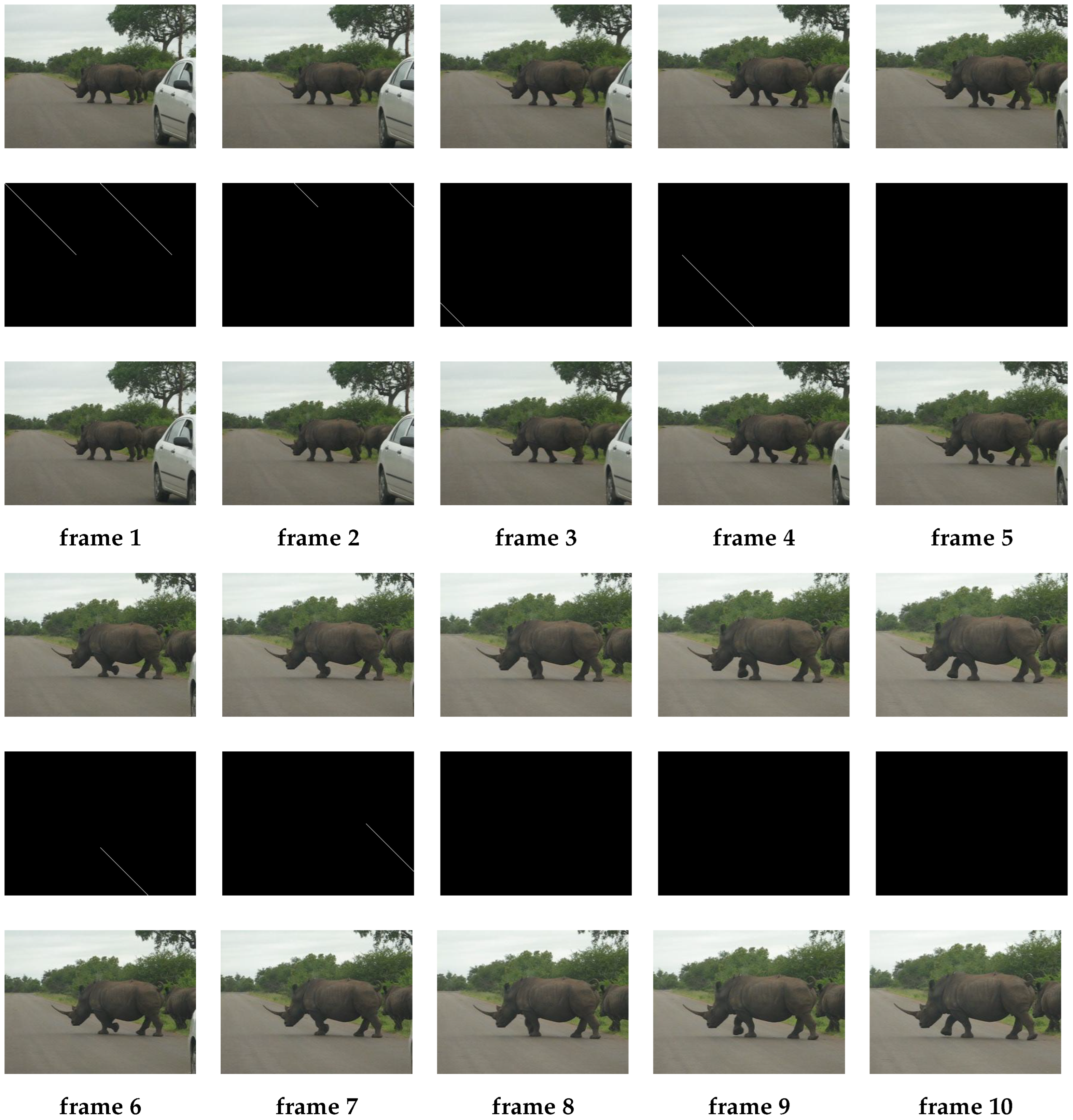
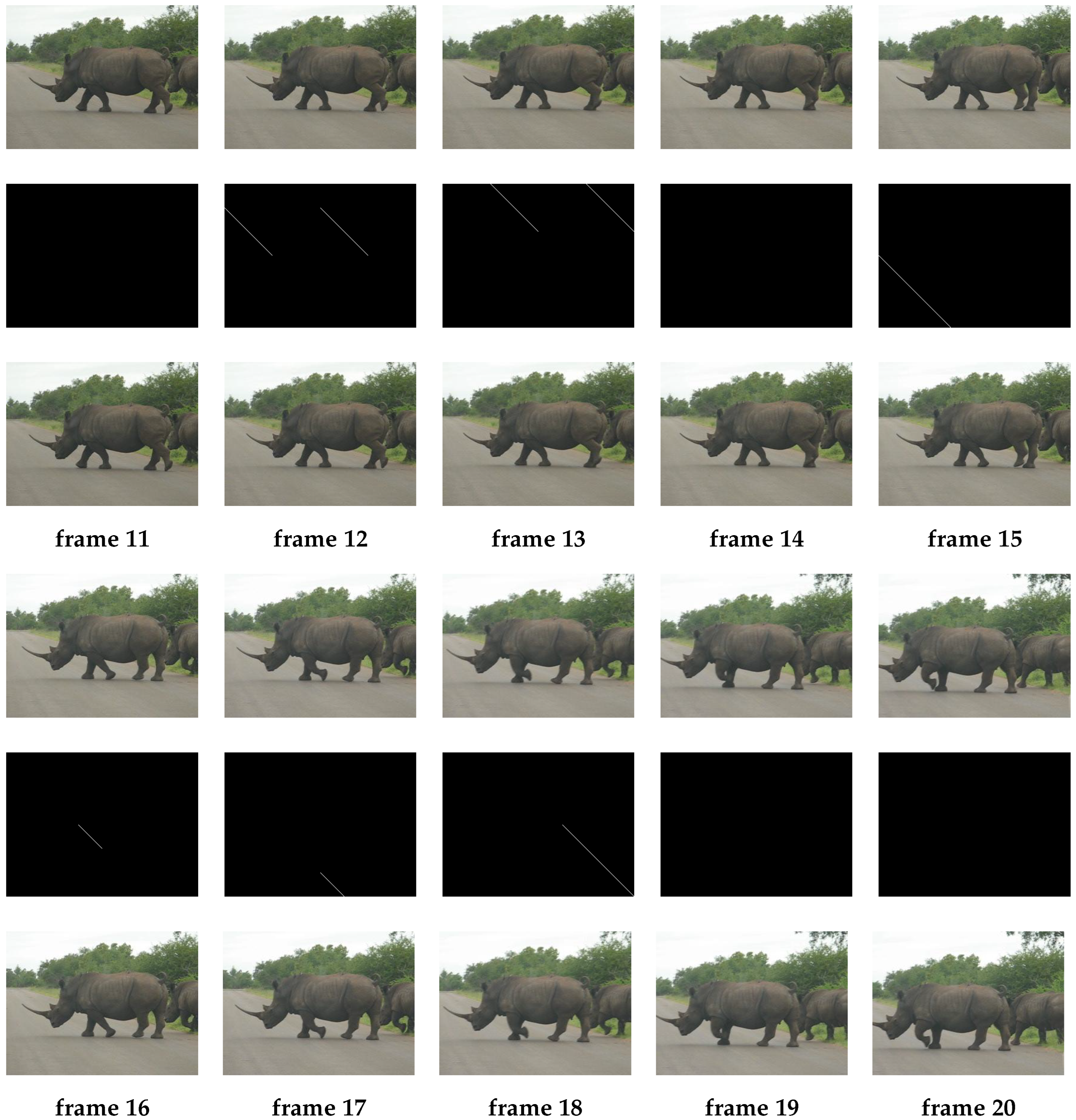
In the experiment, we used the first 20 frames of the color video rhinos.avi from MATLAB R2022a as the original video. Each frame is of size . This color video can be represented as . We performed the Haar discrete wavelet transform and obtained four sub-bands of the same sizes . Then, we applied the simultaneous decomposition for four tensors to obtain the encrypted video and keys. Finally, we used the keys to decrypt the encrypted video.
The results of the encryption and the decryption are shown in
Figure 1 and
Figure 2. It can be seen that each frame of the encrypted video is a binary image, which only has white and black pixels. Therefore, the information of the original video is highly concealed through the encryption process. Furthermore, the decrypted video is almost identical to the original one, which shows that the decryption effect is also great.
It is worth noting that DWT is also useful in color video compression. Hence, our framework can also realize simultaneously encryption and compression. Moreover, we can perform DWT more times in the first step of encryption to shrink the size of the original video and find a balance between speed and effect.
| Algorithm 1: Encryption process |
Input: Original video . Output: Encrypted video and keys , . - 1
For , perform DWT to each frame of the original video. The obtained LL, LH, HL and HH sub-bands of each frame form four sub-videos . - 2
By Theorem 1, compute the simultaneous decomposition - 3
Save and as keys and the encrypted video is the combination of the equivalence canonical form .
|
| Algorithm 2: Decryption process |
Input: Encrypted video and keys , . Output: Decrypted video . - 1
Seperate the encrypted video into four quarters . - 2
Use the keys to decrypt the four quarters: - 3
Apply inverse DWT on and to reconstruct the video .
|
5. Conclusions
We have reviewed results in relation to the Einstein product of tensors and provided a more precise definition of transformation (
1). We have derived a simultaneous decomposition for a quaternion tensor quaternity in Theorem 1 that brings the given tensors into a canonical form with only 0 and 1 entries. The structure of the canonical form has been discussed in detail in Theorem 2 as well. Furthermore, we have applied the proposed simultaneous decomposition combined with DWT to construct a new framework of color video encryption and decryption. The framework can realize simultaneous encryption and compression.
Author Contributions
Conceptualization, J.-W.H. and Y.-Z.X.; methodology, J.-W.H. and Y.-Z.X.; software, J.-W.H. and Y.-Z.X.; validation, J.-W.H., Y.-Z.X. and Z.-H.H.; formal analysis, J.-W.H. and Y.-Z.X.; writing—original draft preparation, J.-W.H. and Y.-Z.X.; writing—review and editing, J.-W.H., Y.-Z.X. and Z.-H.H.; supervision, Z.-H.H.; funding acquisition, Z.-H.H. All authors have read and agreed to the published version of the manuscript.
Funding
This research is supported by the National Natural Science Foundation of China [grant numbers 12271338, 12371023, and 12426508] and Shanghai Oriental Talent Program (Youth Program).
Data Availability Statement
The original contributions presented in this study are included in the article; further inquiries can be directed to the corresponding author.
Conflicts of Interest
The authors declare no conflicts of interest.
References
- Cichocki, A.; Zdunek, R.; Phan, A.H.; Amar, S.I. Nonnegative Matrix and Tensor Factorizations: Applications to Exploratory Multi-Way Data Analysis and Blind Source Separation; John Wiley and Sons: Hoboken, NJ, USA, 2009. [Google Scholar]
- Omberg, L.; Golub, G.H.; Alter, O. A tensor Higher-order singular value decomposition for integrative analysis of DNA microarray data from different studies. Proc. Natl. Acad. Sci. USA 2007, 104, 18371–18376. [Google Scholar] [CrossRef] [PubMed]
- Navasca, C.; De Lathauwer, L.; Kindermann, S. Swamp reducing technique for tensor decomposition. In Proceedings of the 16th European Siganl Processing Conference, Lausanne, Switzerland, 25–29 August 2008. [Google Scholar]
- Shashua, A.; Hazan, T. Non-negative tensor factorization with applications to statistics and computer vision. In Proceedings of the ICML 2005: Proceedings of the 22nd International Conference on Machine Learning, Bonn, Germany, 7–11 August 2005; pp. 792–799. [Google Scholar]
- De Lathauwer, L.; De Moor, B.; Vandewalle, J. A multilinear singular value decomposition. SIAM J. Matrix Anal. Appl. 2000, 21, 1253–1278. [Google Scholar] [CrossRef]
- Brazell, M.; Li, N.; Navasca, C.; Tamon, C. Solving multilinear systems via tensor inversion. SIAM J. Matrix Anal. Appl. 2013, 34, 542–570. [Google Scholar] [CrossRef]
- Ding, W.Y.; Qi, L.Q.; Wei, Y.M. M-tensors and nonsingular M-tensors. Linear Algebra Appl. 2013, 439, 3264–3278. [Google Scholar] [CrossRef]
- He, Z.H.; Ng, M.K.; Zeng, C. Generalized singular value decompositions for tensors and their applications. Numer. Math. Theor. Meth. Appl. 2021, 14, 692–713. [Google Scholar]
- Zeng, C.; Ng, M.K. Decompositions of third-order tensors: HOSVD, T-SVD, and beyond. Numer. Linear Algebra Appl. 2020, 27, e2290. [Google Scholar] [CrossRef]
- Kolda, T.G.; Bader, B.W. Tensor decompositions and applications. SIAM Rev. 2009, 51, 455–500. [Google Scholar] [CrossRef]
- Rodman, L. Topics in Quaternion Linear Algebra; Princeton University Press: Princeton, NJ, USA, 2014. [Google Scholar]
- Zhang, F. Quaternions and matrices of quaternions. Linear Algebra Appl. 1997, 251, 21–57. [Google Scholar] [CrossRef]
- Jia, Z.; Ng, M.K.; Song, G.J. Lanczos method for large-scale quaternion singular value decomposition. Numer. Algorithms 2019, 82, 699–717. [Google Scholar] [CrossRef]
- Jia, Z.; Ng, M.K. Structure preserving quaternion generalized minimal residual method. SIAM J. Matrix Anal. Appl. 2021, 42, 616–634. [Google Scholar] [CrossRef]
- Le Bihan, N.; Sangwine, S. Quaternion principal component analysis of color images. In Proceedings of the 2003 International Conference on Image Processing (Cat. No.03CH37429), Barcelona, Spain, 14–17 September 2003; p. I-809. [Google Scholar]
- Zhang, X.F.; Li, T.; Ou, Y.G. Iterative solutions of generalized sylvester quaternion tensor equations. Linear Multilinear Algebra 2023, 72, 1259–1278. [Google Scholar] [CrossRef]
- Kyrchei, I. Determinantal representations of solutions to systems of quaternion matrix equations. Adv. Appl. Clifford Algebra 2018, 28, 23. [Google Scholar] [CrossRef]
- Zhang, Y.; Wang, R.H. The exact solution of a system of quaternion matrix equations involving η-Hermicity. Appl. Math. Comput. 2013, 222, 201–209. [Google Scholar] [CrossRef]
- Qi, L.; Luo, Z.; Wang, Q.W.; Zhang, X. Quaternion matrix optimization: Motivation and analysis. J. Optim. Theory Appl. 2022, 193, 621–648. [Google Scholar] [CrossRef]
- Pei, S.C.; Cheng, C.M. A novel block truncation coding of color images by using quaternion-moment-preserving principle. IEEE Int. Symp. Circuits Syst. 1996, 2, 684–687. [Google Scholar]
- Miao, J.; Kou, K.I.; Cheng, D.; Liu, W. Quaternion higher-order singular value decomposition and its applications in color image processing. Inf. Fusion 2023, 92, 139–153. [Google Scholar] [CrossRef]
- He, Z.H.; Liu, T.T.; Wang, X.X. Eigenvalues of quaternion tensors: Properties, algorithms and applications. Adv. Appl. Clifford Algebr. 2025, 35, 4. [Google Scholar] [CrossRef]
- He, Z.H.; Chen, C.; Wang, X.X. A simultaneous decomposition for three quaternion tensors with applications in color video signal processing. Anal. Appl. 2021, 19, 529–549. [Google Scholar] [CrossRef]
- He, Z.H.; Navasca, C.; Wang, X.X. Decomposition for a quaternion tensor triplet with applications. Adv. Appl. Clifford Algebr. 2022, 32, 9. [Google Scholar] [CrossRef]
- Einstein, A. The foundation of the general theory of relativity. In The Collected Papers of Albert Einstein 6; Kox, A.J., Klein, M.J., Schulmann, R., Eds.; Princeton University Press: Princeton, NJ, USA, 2007; pp. 146–200. [Google Scholar]
- He, Z.H.; Navasca, C.; Wang, Q.W. Tensor decompositions and tensor equations over quaternion algebra. arXiv 2017, arXiv:1710.07552v1. [Google Scholar]
- Wang, Q.W.; Zhang, X.; van der Woude, J.W. A new simultaneous decomposition of a matrix quaternity over an arbitrary division ring with applications. Commun. Algebra 2012, 40, 2309–2342. [Google Scholar] [CrossRef]
- He, Z.H.; Wang, Q.W.; Zhang, Y. The complete equivalence canonical form of four matrices over an arbitrary division ring. Linear Multilinear Algebra 2018, 66, 74–95. [Google Scholar] [CrossRef]
- Lai, C.C.; Tsai, C.C. Digital image watermarking using discrete wavelet transform and singular value decomposition. IEEE Trans. Instrum. Meas. 2010, 59, 3060–3063. [Google Scholar] [CrossRef]
| Disclaimer/Publisher’s Note: The statements, opinions and data contained in all publications are solely those of the individual author(s) and contributor(s) and not of MDPI and/or the editor(s). MDPI and/or the editor(s) disclaim responsibility for any injury to people or property resulting from any ideas, methods, instructions or products referred to in the content. |
© 2025 by the authors. Licensee MDPI, Basel, Switzerland. This article is an open access article distributed under the terms and conditions of the Creative Commons Attribution (CC BY) license (https://creativecommons.org/licenses/by/4.0/).

