Parametric Analysis of Auxetic Honeycombs

Abstract

The auxetic honeycomb can change mechanical behavior from positive to negative Poisson’s ratio by slightly adjusting the geometrical feature. As a first step, the paper investigates existing analytical solutions to the problem to provide the theoretical background. The present study discusses the methodology used to examine these structures using the finite element method and how to adapt simple numerical models to capture structural behavior. Subsequently, the numerical model is used to run parametric analyses to determine the performance and provide the background for discussing the influence of the dimensional set on the response. Following this set of observations, an empirical solution connecting the unit cell to the global structure was formulated. A large dataset is generated to train and check machine-learning applications to develop a helpful tool for predicting the response without numerical and theoretical evaluation models and methods. The machine-learning section investigates the influence of several parameters on the response and the effect of complete versus incomplete datasets.

1. Introduction

The Negative Poisson’s ratio exhibits unique mechanical properties, such as expansion when stretched, which contrasts with conventional materials [1]. The first investigations detailed the behavior of cellular materials [2,3]. There is great potential for NPR materials to enhance functionality and performance in various fields while also addressing the challenges in their manufacturing [4] and application [5] in this world and beyond [6].

The review performed by Li et al. [7] highlights the modeling and development of auxetic foams and their applications in fields like aerospace, biomedical devices, sports [8], and textiles [9,10]. Wang et al. [11] report valuable results obtained using a hybrid configuration of a re-entrant and chiral structure to improve the wing design. It details the structural designs of auxetic materials, such as re-entrant and chiral structures, and their mechanical properties, including high indentation resistance and fracture toughness. Customized design can be manufactured using additive manufacturing [12,13] in creating these materials, emphasizing the importance of hierarchical designs and soft auxetic mechanical metamaterials [14,15,16]. The effect of printing methods and materials on the mechanical performance of re-entrant auxetic structures was investigated by Dong et al. [17]. Experimental results revealed that peak force and energy absorption, influenced by printing direction, can be improved by proper adjustments. There are also conventional manufacturing methods that can produce re-entrant structures, as demonstrated by Tian et al. [18].

Szeles et al. [19] proposed an update to the conventional configuration of the re-entrant structure. Their work was focused on a novel filled doubly re-entrant auxetic lattice structure designed for impact absorption. This structure, modified with silicone fillings, enhances energy dissipation during impacts. A variant of the re-entrant lattice structure developed for increased stiffness was investigated by Chen et al. [20] The solution proposes using additional ligaments to increase stiffness. The paper introduces the ligament modeling procedure using Euler—Bernoulli beams, considering the ligaments’ slender configuration.

A combination of standard honeycomb and re-entrant was investigated by Panowicz et al. [21] as a solution for a new auxetic configuration, while re-entrant embedded in a hexagonal honeycomb was investigated by Peng et al. [22] in a search for improved mechanical properties of the structure. Nature provides valuable information on the efficiency of structures. Zhang et al. investigated a structure with curved ligaments [23] under impact loading to prove the efficacy of the design. Quasi-static loading conditions [24,25,26,27] are often used as an experimental investigation method. The dynamics of compressive behavior [28] of cellular materials was investigated by Sun and Li [29] to determine the methods and results under high strain rates. Furthermore, analytical and numerical solutions by Ma and Zhang investigated the nonlinear behavior of re-entrant structures under increased loads [30] to complete the potential field of application for these structures.

A variant of a re-entrant structure in the shape of the auxetic star was introduced by Ai and Gao [31]. The paper explores the methods used to derive an analytical solution for Poisson’s ratio and provides a detailed investigation of the importance of the design parameters.

The 2D re-entrant structures can be arranged in a 3D configuration to further enhance the mechanical performance of structures—the work of Jiang et al. [32] discuss the performance of a 3D re-entrant circular auxetic metamaterial. Thus, Luo et al. [33] investigated the re-entrant cell combined with face-centered cubic elements to improve the performance under compressive loads.

Bora et al. [34] demonstrated that a change in the geometrical definition of geometry from sharp to rounded corners can provide interesting updates on mechanical performance. At the same time, the re-entrant unit was combined with properly arranged ligaments by Zhang et al. [35] to explain the behavior under large deformations [36].

The experimental methods are necessary for the validation process of numerical models. Schürger et al. [37] investigated re-entrant auxetic structures using photoelasticity to provide detailed information capable of augmenting numerical results.

The homogenization method [38,39] can provide further applications that are critical in terms of computational resources. Gunaydin et al. [40] developed a model dedicated to re-entrant and honeycomb structures based on finite element simulations.

Machine learning methods [41] applied to improve the design of re-entrant-like structures manufactured by additive methods, were investigated by Hasanzadeh [42].

The search for improved configurations based on the re-entrant unit cell is an ongoing process that keeps the researcher focused on this topic and the imagination running for enhanced configurations.

The design of the honeycomb is relatively simple, yet due to the change in the displacement behavior from positive to negative Poisson’s ratio, it can provide a near-zero [21] or composite behavior [43].

The present work is focused on the potential performance of the honeycomb structures for further development and on investigating the Poisson’s ratio, considering requirements related to the geometry and displacement of the structures under applied loads. Literature [20,35,44] provides methods for investigating the apparent Young and shear moduli once it is decided that the structure is designed according to the environment.

2. Modelling: Analytical and Numerical Formulations

2.1. Theoretical Background

Gibson et al. [2] investigated the mechanical behavior of honeycomb structures and provided a solution for the structural performance parameters.

Figure 1 presents the geometrical features of the honeycomb cell (a) and a variant defined as re-entrant (b).

To determine an analytical solution, the standard beam formulation was applied with the amendment of neglecting the shear stress. Thus, the solution for Poisson’s ratio was obtained as follows:

$${\nu }_{12}={\displaystyle \frac{\left(H/l+\mathit{sin}\theta \right)·\mathit{sin}\theta }{{\cos }^2\theta }}$$

(1)

where dimension $l$ is defined by:

$$l=\sqrt{{\left({\displaystyle \frac{L}{2}}\right)}^2+{\left({\displaystyle \frac{H}{2}}-{\displaystyle \frac{h}{2}}\right)}^2}$$

(2)

Dimension $L$ defines the length of unit cell in horizontal direction $\left(1\right)$, dimension $H$ defines the length of the vertical ligament of cell, dimension $h$ defines the inner gap measure on vertical direction $\left(1\right)$ while dimension $l$ defines the length of ligament position and the angle $\theta$ from the horizontal axis. The value of $h$ should be considered according to the sign of $\theta$, considering the notation convention presented in Figure 1.

The investigations were further extended by Masters & Evans [44], considering the complex deformation mechanics of the ligaments, which include flexure, stretching, and hinging [45]. The solution obtained by solving the complex set of equations is therefore defined by:

$${\nu }_{12}=-\sin \theta ·\left({\displaystyle \frac{H}{l}}+\sin \theta \right)·\left[{\displaystyle \frac{-\frac{1}{K_f}-\frac{1}{K_h}+\frac{1}{K_s}}{\frac{{\cos }^2\theta }{K_f}+\frac{{\cos }^2\theta }{K_h}+\frac{2·H/l+{\sin }^2\theta }{K_s}}}\right]$$

(3)

while introducing the following coefficients:

$$\begin{gathered} K_f={\displaystyle \frac{E_0·w·t^3}{l^3}} \\ {K}_h={\displaystyle \frac{G_0·w·t}{l}} \\ {K}_s={\displaystyle \frac{E_0·w·t}{H}} \\ {G}_0={\displaystyle \frac{E_0}{2·\left(1+{\nu }_0\right)}} \end{gathered}$$

(4)

In the equations mentioned above $E_0$, $G_0$, ${\nu }_0$ denotes the parameters of the base material used to manufacture the cell, $t$ is the thickness of the ligaments and $w$ is the width of the structure.

2.2. Finite Elements Model

Structural finite element analysis can provide reliable results, and the method can be easily implemented by programming a planar or 2D analysis. A MATLAB software application was developed following the principles of 2D beam elements [46].

The theorem of the minimum potential energy gives:

$${\displaystyle \frac{\partial \mathrm{U}}{\partial Q_i}}=0$$

(5)

where $Q_i$ is the vector of nodal displacements.

The general formulation expressed by the matrix form [47]:

$$\left(\underset{V}{\iiint }{\left[B\right]}^T·\left[E\right]·\left[B\right]·dV\right)·\overrightarrow{Q}=\overrightarrow{F}$$

(6)

is reduced for the implicit analysis as:

$${\overrightarrow{F}}^g=\left[K^e\right]·{\overrightarrow{Q}}^g$$

(7)

where ${\overrightarrow{F}}^g$ is the vector of applied nodal forces; $\left[K^e\right]$ defines the stiffness matrix for the global coordinate frame and ${\overrightarrow{Q}}^g$ is the vector of nodal displacements.

The global stiffness matrix is a collection of local stiffness matrices aligned with the global coordinate frame by using the transformation matrix $\left[T\right]$:

$$\left[K^e\right]={\left[T\right]}^T·\left[k^e\right]·\left[T\right]$$

(8)

The element’s stiffness matrix, in the local coordinate system, is defined by:

$$\left[k^e\right]=\underset{V_e}{\iiint }{\left[B\right]}^T·\left[E\right]·\left[B\right]·dV$$

(9)

where $\left[B\right]$ is the displacement matrix and $\left[E\right]$ is the elasticity matrix.

For the planar frame element, the stiffness matrix reduces to:

$$\left[k^e\right]=E·{\int }_0^{l_e}dx\underset{A}{\iint }{\left[B\right]}^T·\left[B\right]·dA$$

(10)

Considering the following definition of the displacement matrix $\left[B\right]$, derived according to the small displacement theory (Bernoulli’s formulation [48,49]):

$$\left[B\right]=\left\{-\begin{array}{cc}\begin{array}{ccc}{\displaystyle \frac{1}{l}}& -{\displaystyle \frac{y}{l^3}}\left(12·x-6·l\right)& -{\displaystyle \frac{y·l}{l^3}}\left(6·x-4·l\right)\end{array}& \begin{array}{ccc}{\displaystyle \frac{1}{l}}& {\displaystyle \frac{y}{l^3}}\left(12·x-6·l\right)& -{\displaystyle \frac{y·l}{l^3}}\left(6·x-2·l\right)\end{array}\end{array}\right\}$$

(11)

the stiffness matrix is defined by:

$$\left[k^e\right]=\left[\begin{array}{cccccc}{\displaystyle \frac{A_e\cdot E_0}{L_e}}& 0& 0& -{\displaystyle \frac{A_e\cdot E_0}{L_e}}& 0& 0\\ 0& {\displaystyle \frac{12\cdot E_0\cdot I_e}{L^3}}& {\displaystyle \frac{6\cdot E_0\cdot I_e}{L_e^2}}& 0& -{\displaystyle \frac{12\cdot E_0\cdot I_e}{L_e^3}}& {\displaystyle \frac{6\cdot E_0\cdot I_e}{L_e^2}}\\ 0& {\displaystyle \frac{6\cdot E_0\cdot I_e}{L_e^2}}& {\displaystyle \frac{4\cdot E_0\cdot I_e}{L_e}}& 0& -{\displaystyle \frac{6\cdot E_0\cdot I_e}{L_e^2}}& {\displaystyle \frac{2\cdot E_0\cdot I_e}{L_e}}\\ -{\displaystyle \frac{A_e\cdot E}{L}}& 0& 0& {\displaystyle \frac{A_e\cdot E_0}{L_e}}& 0& 0\\ 0& -{\displaystyle \frac{12\cdot E_0\cdot I_e}{L_e^3}}& -{\displaystyle \frac{6\cdot E_0\cdot I_e}{L_e^2}}& 0& {\displaystyle \frac{12\cdot E_0\cdot I}{L_e^3}}& -{\displaystyle \frac{6\cdot E_0\cdot I_e}{L_e^2}}\\ 0& {\displaystyle \frac{6\cdot E_0\cdot I_e}{L_e^2}}& {\displaystyle \frac{2\cdot E_0\cdot I_e}{L_e}}& 0& -{\displaystyle \frac{6\cdot E_0\cdot I}{L_e^2}}& {\displaystyle \frac{4\cdot E_0\cdot I_e}{L_e}}\end{array}\right]$$

(12)

where $I_e={\iint }_{A_e}{y}^2·dA$ is the moment of inertia.

The rotation matrix for the planar frame element is defined by:

$$\left[T\right]=\left[\begin{array}{cccccc}\cos {\theta }_e& -\sin {\theta }_e& 0& 0& 0& 0\\ \sin {\theta }_e& \cos {\theta }_e& 0& 0& 0& 0\\ 0& 0& 1& 0& 0& 0\\ 0& 0& 0& \cos {\theta }_e& -\sin {\theta }_e& 0\\ 0& 0& 0& \sin {\theta }_e& \cos {\theta }_e& 0\\ 0& 0& 0& 0& 0& 1\end{array}\right]$$

(13)

where ${\theta }_e$ is the angle measure between the local coordinate frame associated with the element and the global coordinate frame.

The model generation method is presented step-by-step in Figure 2.

The coincident nodes and overlapped beams are merged during the numerical model generation process, defining a consistent numerical model [46]. Furthermore, the ligaments are assigned to different parts to allow various dimensional parameters (Figure 2g).

As an additional feature, a stiff beam (with a Young modulus 10 times higher in magnitude compare to the base material and a high value for the height of the cross-section) can connect the top and/or bottom nodes to replicate experimental loading conditions as the moving and fixed plattens of the testing machine (Figure 2h).

The dimensions of the beam elements assigned to each geometrical feature can be defined as equal length or progressive as a function of the spacing ratio $\left(r_e\right)$.

The normalized dimension of the current of the beam elements $\left(\overline{l_e}\right)$ is determined as a function of the normalized length $\left(\overline{l}\right)$ defined as:

$$\begin{gathered} \overline{l_{e,i}}=\overline{l}-\left(⌈{\displaystyle \frac{n_2}{2}}⌉-i\right)·r_e \\ \overline{l}={\displaystyle \frac{n_e}{2}}+{\displaystyle \frac{1}{2}}·r_e·\left({\displaystyle \frac{n_e}{2}}-1\right) \end{gathered}$$

(14)

where $n_e$ is the number of elements assigned to the geometrical element. The node distribution is symmetric about the midpoint of the ligament.

Figure 3 presents the method for equally (a) and progressively increasing element sizes (b).

3. Results

This section will discuss preliminary results based on theoretical and numerical modeling.

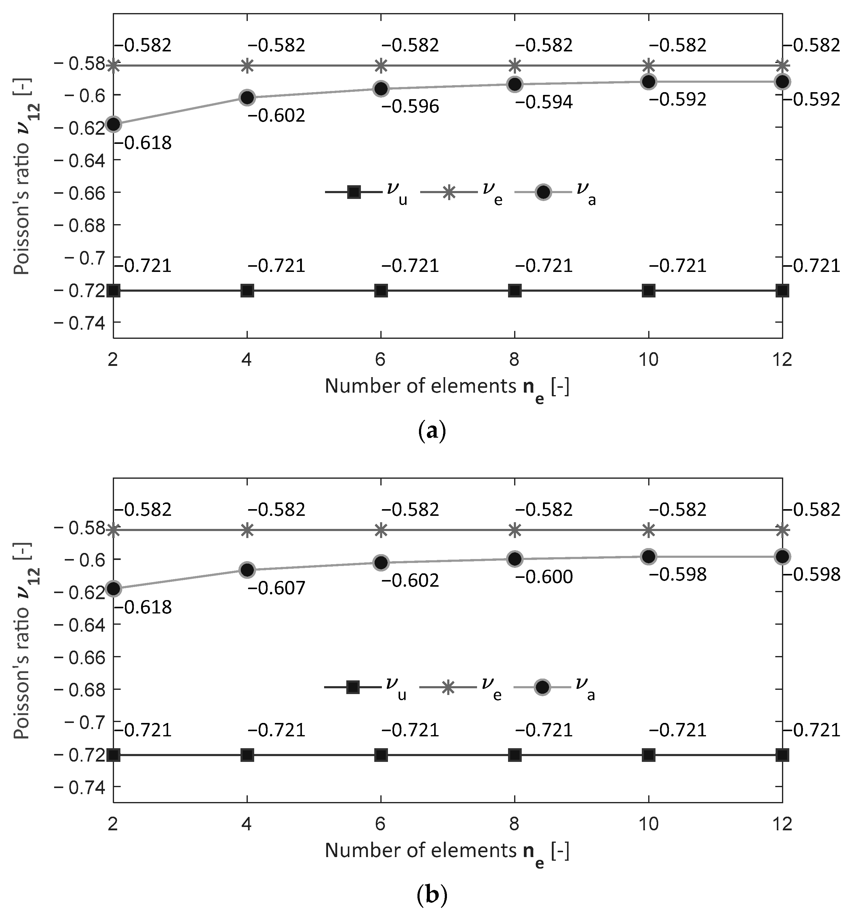
3.1. Validation of the Numerical Model—Convergence Analysis

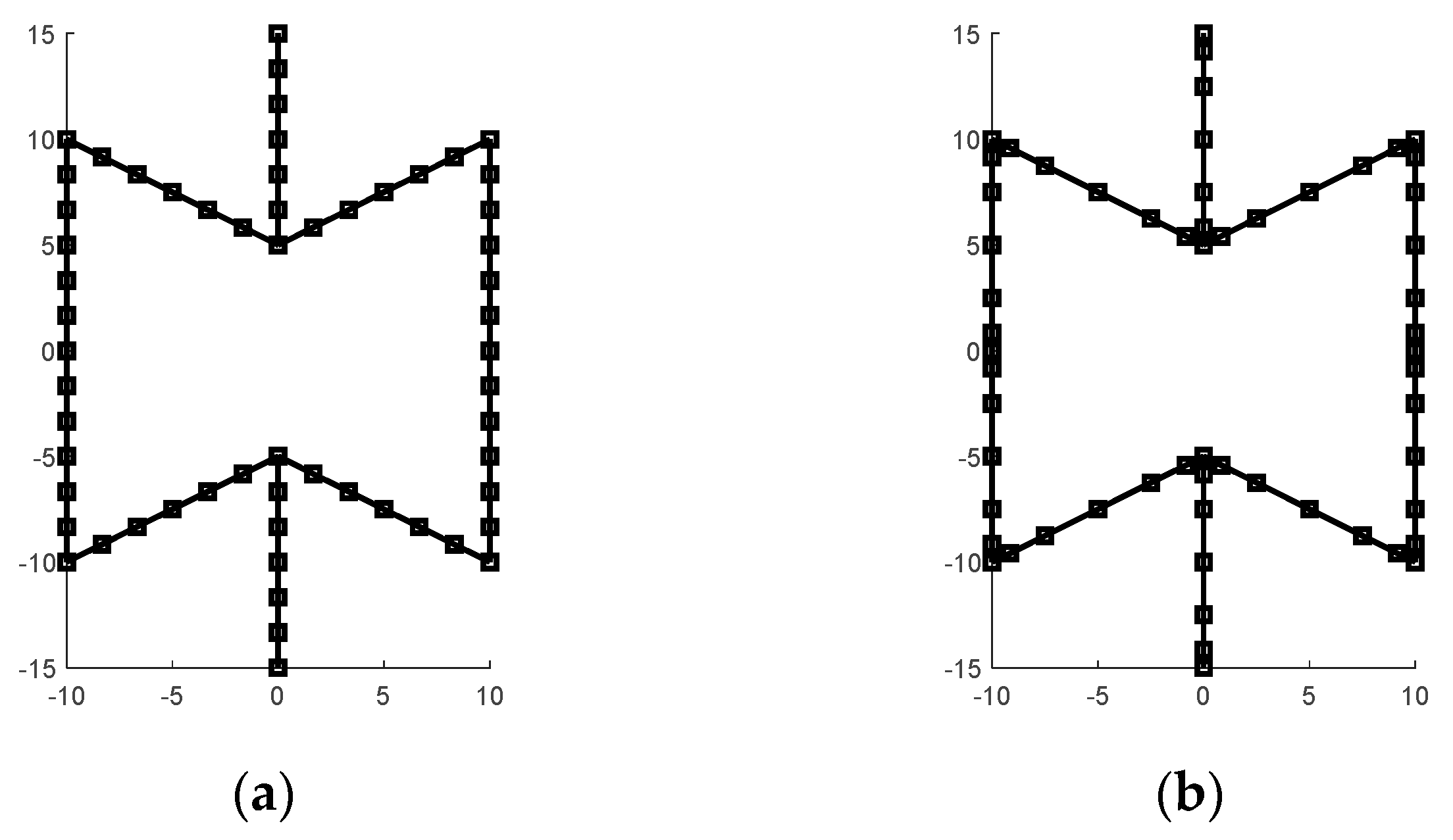
The previous section discussed a series of features implemented on the numerical model. The procedure for the calculation of Poisson’s ratio is implemented for three levels:

• cell level $\left({\nu }_u\right)$: for the central feature, two pairs of nodes are identified: the first one is located at the midpoint of the vertical ligaments, while the second pair is located at the convergence of the horizontal (or inclined) ligaments (Figure 2f);
• structure level—maximum displacement $\left({\nu }_e\right)$: two pairs of nodes are defined: the first pair is defined by the nodes located on the left and right side at the middle of the structure, while the second pair is defined by points located on top and bottom of the structure (Figure 2f);
• structure level—average displacement $\left({\nu }_a\right)$. The averaged displacements [20] of the nodes located on the left and right sides are evaluated to define the first pair of coordinates. The second dimension is defined by nodes located on the top and bottom of the structure.

Results presented in Figure 4 reveal that by using 6 elements $\left(n_e\right)$ per ligament with a progression factor $\left(r_e\right)$ of 3, the numerical values reported are within a close tolerance $\left(0.004\right)$ to a model with a higher number of elements per ligament $\left(n_e\ge 8\right)$.

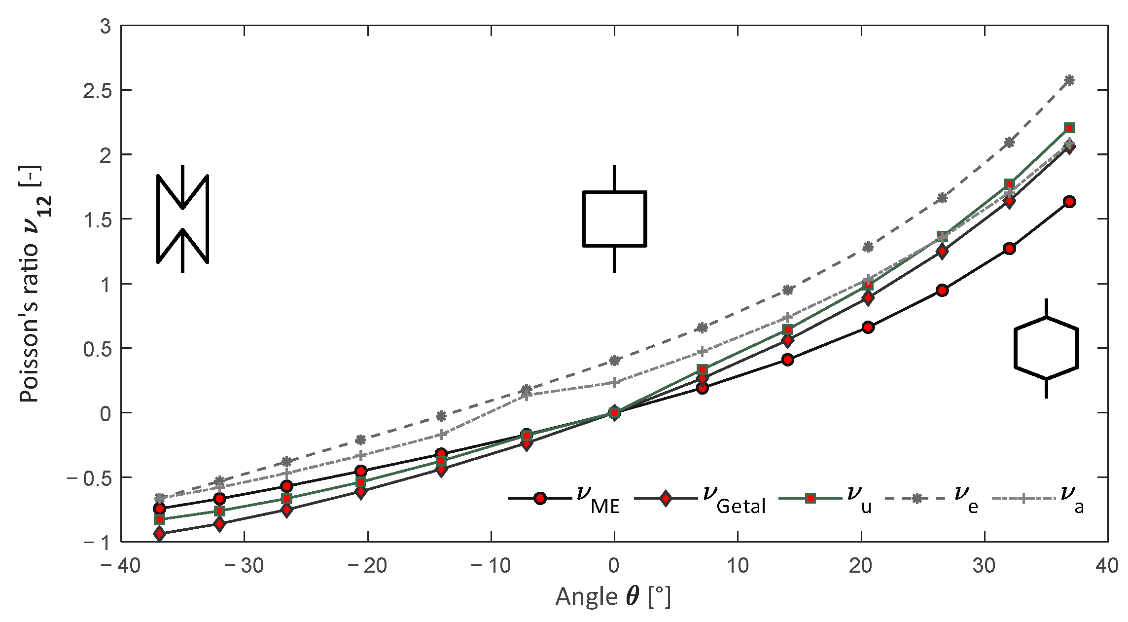
3.2. Analytical vs. Numerical Solution

The results of Equations (1) and (3) are compared with the solution provided by the numerical model.

Results displayed in Figure 5 reveal that the solution obtained using the numerical solution agrees with the analytical formulation provided by Masters & Evans. It is worth noting that the analytical solution slightly overestimates the results for the re-entrant configuration and reverses the tendency.

3.3. Experimental Work

A sample structure was manufactured using Additive Manufacturing [50,51] method by a stereolithography (SLAP) printer (Anycubic Photon M5, Shenzhen Anycubic Technology Co., Shenzhen, China). The part was subsequently washed and cured (Anycubic Wash & Cure 2.0) to improve the mechanical performance. The material selected is an ABS resin. The physical and mechanical properties of the resin are listed in

Table 1. Anycubic ABS-like resin. Physical and mechanical properties.

Specification	Data
Density	$1.05–1.25 \mathrm{g}/{\mathrm{c}\mathrm{m}}^3$
Flexural modulus	$1400–1600 \mathrm{M}\mathrm{P}\mathrm{a}$
Flexural strength	$50–60 \mathrm{M}\mathrm{P}\mathrm{a}$
Tensile strength	$35–55 \mathrm{M}\mathrm{P}\mathrm{a}$
Elongation at break	$20–30\%$

.

The finished part was tested under compressive load using a computerized universal testing machine (class $0.5$/max. load $50 \mathrm{k}\mathrm{N}$). The structure was loaded up to $1.0 \mathrm{k}\mathrm{N}$ and subsequently unloaded with the speed of the moving head of $5.0 \mathrm{m}\mathrm{m}/\mathrm{m}\mathrm{i}\mathrm{n}$, and the cycle was repeated 3 times. A series of markers was applied to the part to allow digital measurements during the experiment. The sample is presented in Figure 6a.

The results presented in this work are part of a larger experimental investigation. However, as the effects of the manufacturing process are not investigated, the structure displaying the most reliable results was selected to demonstrate the existence of analytical results. The processing procedure, further discussed, can be successfully used for experimental investigations.

Digital images of the structures were captured during the loading process (for the second cycle to avoid structure misalignment), allowing further investigation [52,53]. The original image was cropped to the dimensions of the central unit (Figure 6b) and converted to a black-and-white image (Figure 6c). The contours were detected (Figure 6d), and the type of features was identified (Figure 6e).

The contour is classified as a circle if each point of the contour collection follows the rule:

$${R_{min}\le d}_{i,c}\le R_{max}$$

(15)

where $d_{i,c}$ is the distance from the current point $i$ to the center of the collection $\left(n_p\right)$:

$$\begin{gathered} x_c={\displaystyle \frac{1}{n_p}}·\sum _1^{n_p}{x}_i \\ {y}_c={\displaystyle \frac{1}{n_p}}·\sum _1^{n_p}{y}_i \\ {d}_{i,c}=\sqrt{{\left(x_i-x_c\right)}^2+{\left(y_i-y_c\right)}^2} \end{gathered}$$

(16)

and $R_{min}$ and $R_{max}$ are user-defined parameters. The algorithm was implemented in a MATLAB application that allows tracking for all images captured during the experimental work (Figure 7).

The experimental value of Poisson’s ratio recorded for the cell is ${\nu }_{u,e}=-0.710,$ while the value determined using the numerical model is ${\nu }_{u,e}=-0.700$ with a difference of $1.4\%$ between the reported values.

4. Discussion

The numerical model is validated against theoretical and experimental data and is capable of being used for extended investigations [35,54,55].

4.1. Configuration of the Structure

The unit cell is stable during loading; however, the global effect depends on the number of cells defined along the horizontal and vertical axes.

Six elements and a progressive distribution of the nodes were used to test the cell’s geometrical features, and a series of structures were tested under compressive loads.

Figure 8 presents the results obtained for the structure’s unit cell (a), edge (b), and average (c) deformations.

As expected, Poisson’s ratio for the unit cell (Figure 8a) is not so influenced by the configuration of the structure. However, the plots presented in Figure 8b,c reveal that Poisson’s ratio is variable with the configuration of the structure.

Values are affected mainly by the number of cells in the vertical direction. An empirical solution for the average deformation of the structure, investigating the connection between the unit cell and the edge value of the number of cells in the vertical direction, can be provided:

$${\nu }_a^{*}={\nu }_u·{\displaystyle \frac{1}{e^{\frac{1}{C_V}}}}$$

(17)

Numerical values are presented in

Table 2. Computed vs. estimated average Poisson’s ratio.

${\mathit{C}}_{\mathit{V}}$	4	5	6	7	8
$L=20 \mathrm{m}\mathrm{m}; H=20 \mathrm{m}\mathrm{m}; h=10 \mathrm{m}\mathrm{m}; t=1.0 \mathrm{m}\mathrm{m}; w=2.0 \mathrm{m}\mathrm{m}$
${\nu }_u$	0.722	0.722	0.722	0.722	0.722
${\nu }_a$	0.575	0.602	0.620	0.634	0.644
${\nu }_a^{*}$	0.652	0.591	0.611	0.626	0.637
$diff \%$	−2.21	−1.81	−1.42	−1.28	−1.06
$L=40 \mathrm{m}\mathrm{m}; H=30 \mathrm{m}\mathrm{m}; h=15 \mathrm{m}\mathrm{m}; t=2.0 \mathrm{m}\mathrm{m}; w=2.0 \mathrm{m}\mathrm{m}$
${\nu }_u$	0.408	0.408	0.408	0.408	0.408
${\nu }_a$	0.329	0.344	0.353	0.362	0.367
${\nu }_a^{*}$	0.318	0.334	0.345	0.354	0.360
$diff \%$	−3.42	−2.89	−2.16	−2.29	−1.89

.

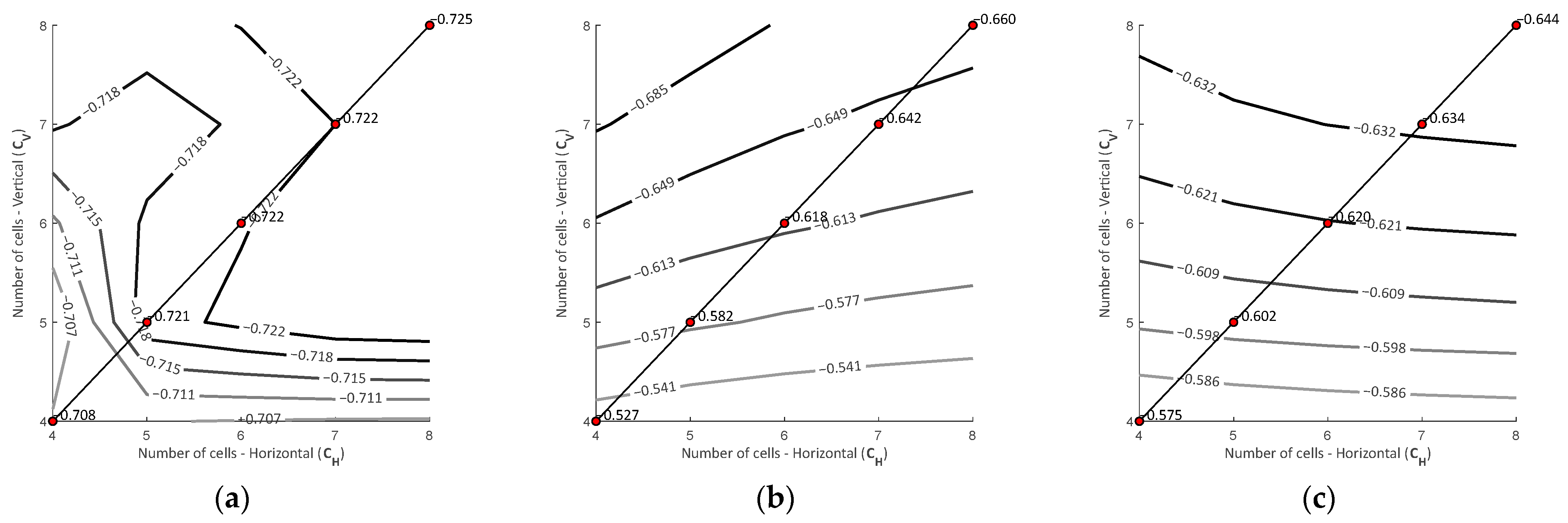
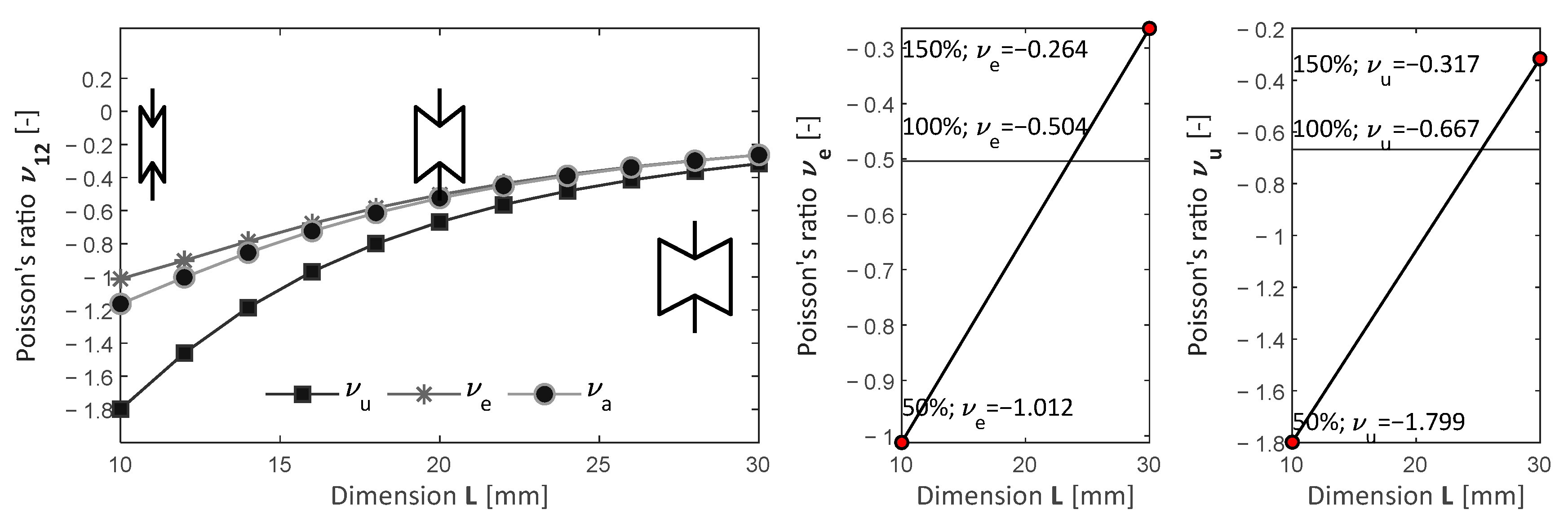
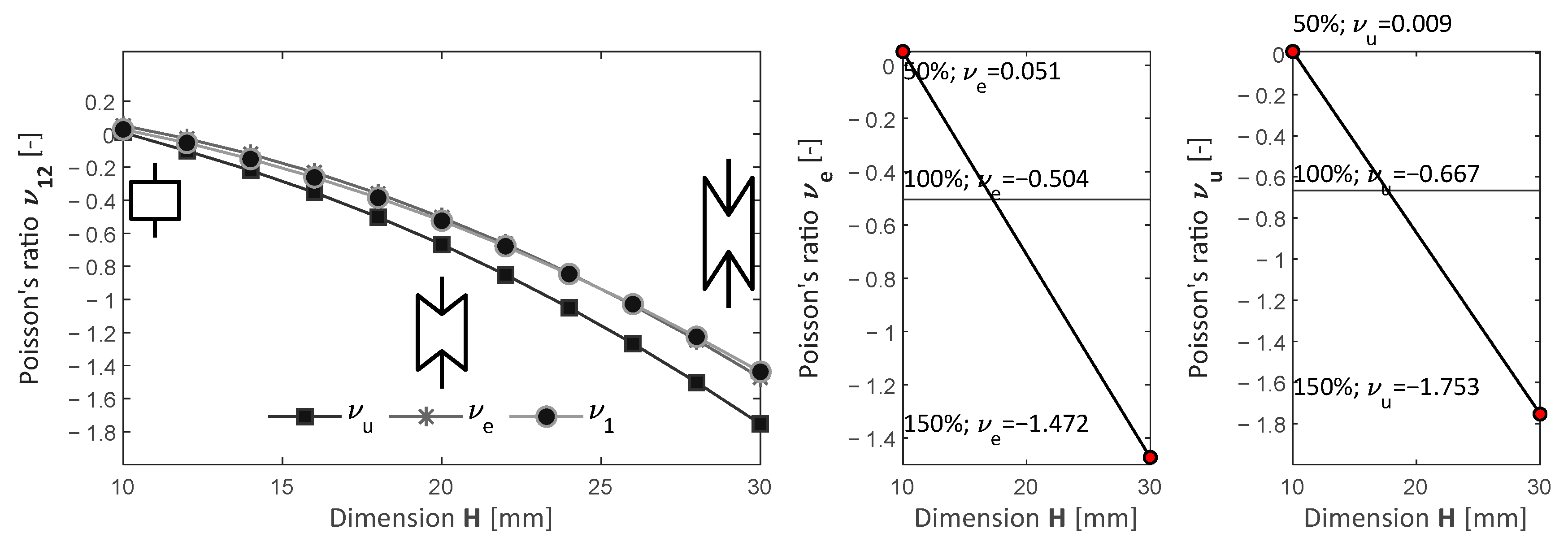
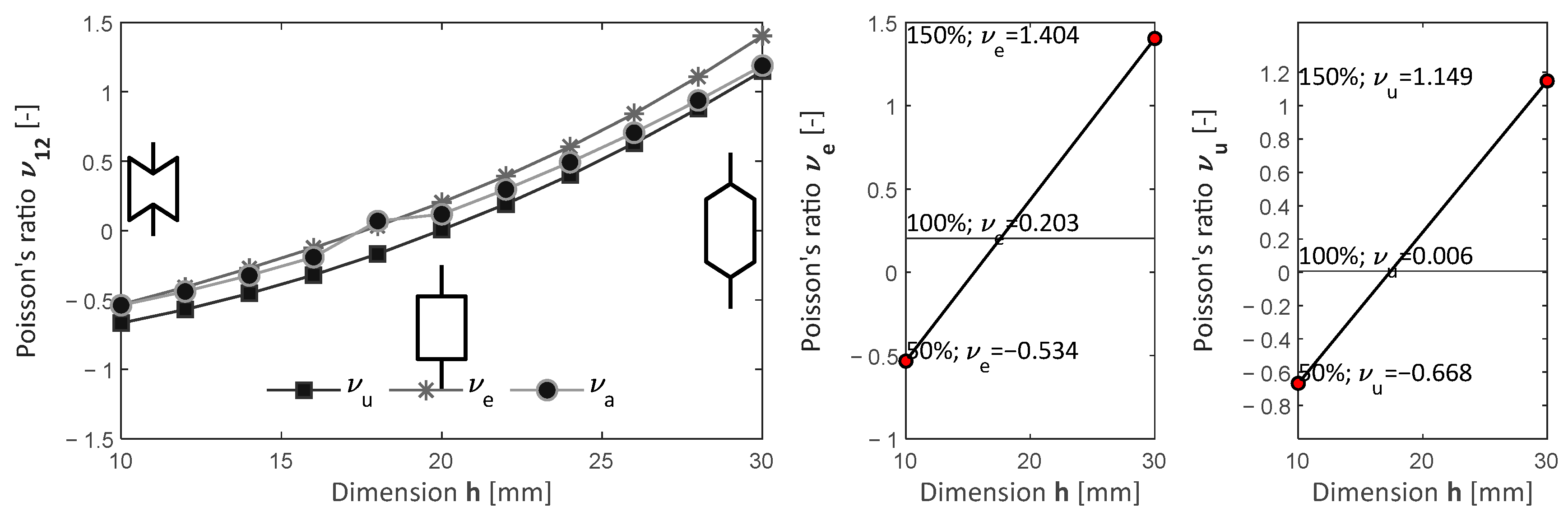
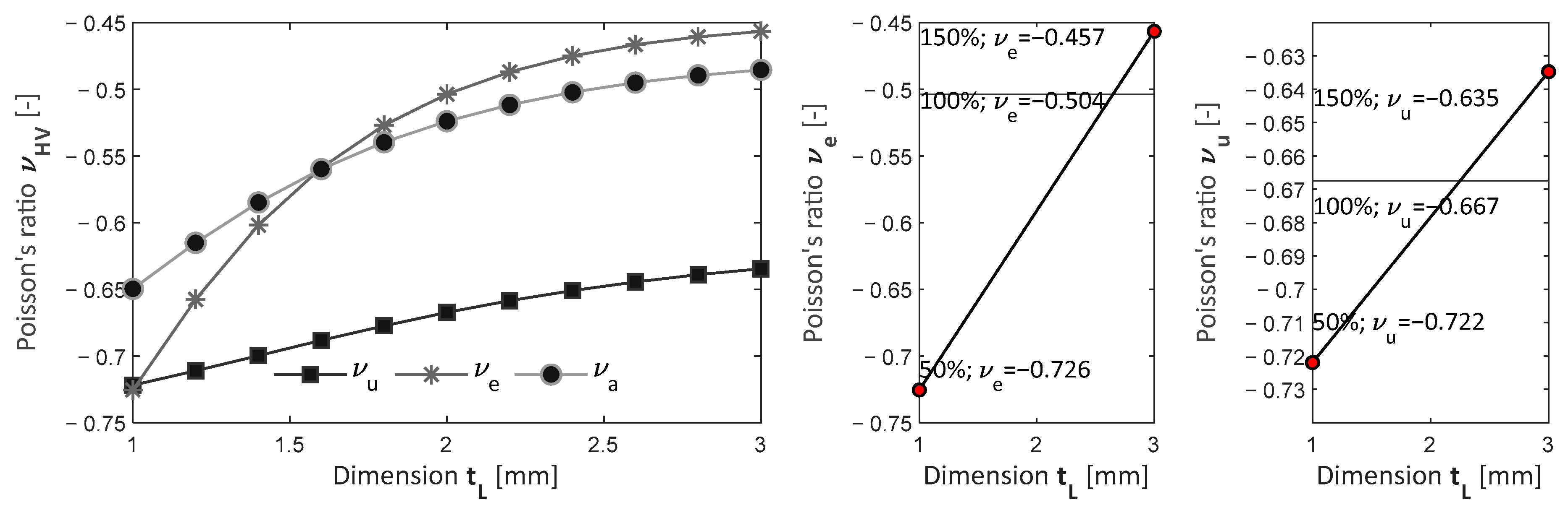
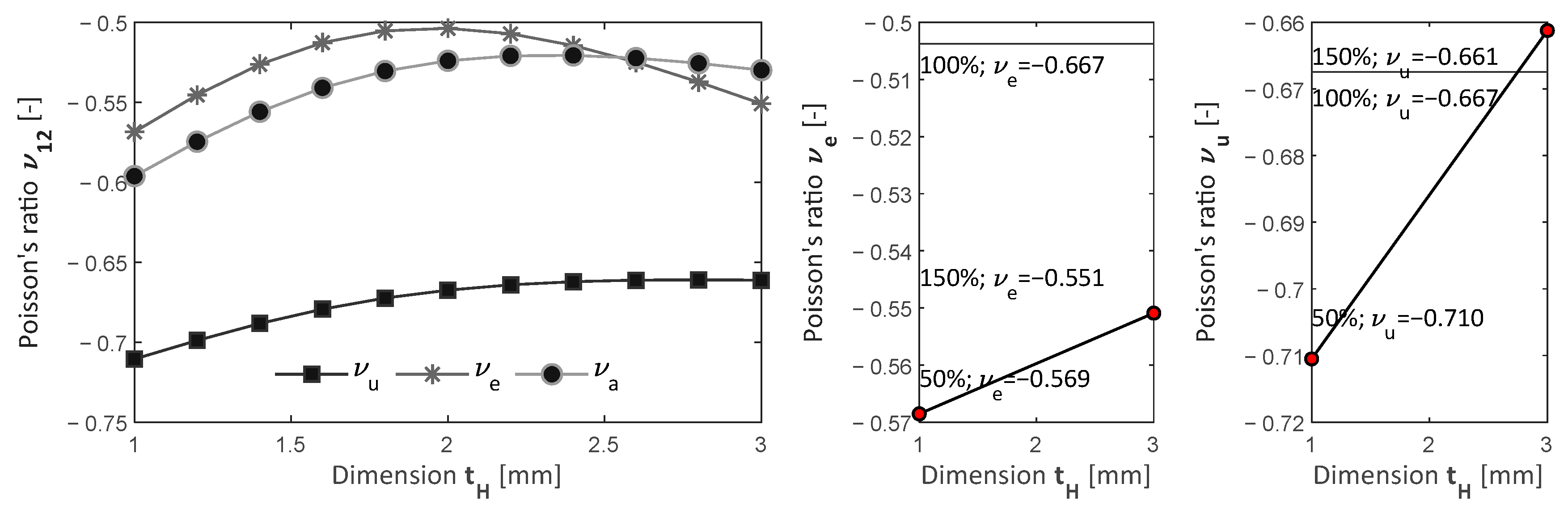
4.2. Parametric Analysis

The reference cell; is determined by $L, H, h$ for the dimensions of the ligaments and $t_L, { t}_H$ for the thickness of the horizontal and vertical ligaments. The set defines the base dimensions $\left[\mathrm{20,20,10,2},2\right] mm$. For each analysis, one dimension can range between $50$ to $200\%$ of the nominal value.

Figure 9 shows the results of the numerical analysis in the case of dimension $H$.

As expected, given the shape of the unit cell, the values of the parameters ${\nu }_u,{\nu }_e$ and ${\nu }_a$ are in the negative range. Once the dimension parameter $L$ decreases for the nominal value there is a fast decrease in Poisson’s ratio to $-1.799$ about $169\%$, while for the wider structures, Poisson’s ratio increases to $-0.317$ a change of $-52\%$ of the value.

The investigations of dimension $H$ gives the response presented in Figure 10.

Poisson’s ratio ranges from $-1.753$ to $0.009$, a change between 162% and −98$\%$ of the reference value, also displaying a positive value for the rectangular-type configuration of the honeycomb. Results presented in Figure 9 and Figure 10 reveal that dimension $L$ defines a broader range of results, thus it can have a greater impact on the mechanical behavior compared to the dimension $H$.

The results obtained for the investigations on the parameter $h$ are presented in Figure 11.

Parameter $h$ gives the most significant change in the response from negative $\left(-0.668\right)$ to positive $\left(1.149\right)$ and can be defined as the primary parameter used to investigate structural behavior.

The analytical solution developed by Masters & Evans [44] includes terms defining the thickness of the bent ligament $\left(t\right)$, subsequently associated with the horizontal ligament $\left(L\right)$.

The evaluated Poisson’s ratio $\left({\nu }_u\right)$ ranges from $-0.722$ to $-0.635$. For the indication, the simulation results are more interesting for the edge measurements ${\nu }_e$ and ${\nu }_a$ because of the existence of the free horizontal edge (Figure 12).

The last parameter investigated is the thickness of the vertical ligament $t_H$.

The effect on the measurements performed on the edges shows an interesting variation (Figure 13). Investigating the impact of the thickness of the vertical ligament at the cell level $\left({\nu }_u\right)$ it can be noticed that an increase gives a stiffer behavior as the base of the horizontal ligament (connection to the vertical ligament) is thicker. On the other hand, the behavior of structure $\left({\nu }_e\right)$ displays a peak value. This is the effect of relative displacement on horizontal direction $\left(1\right)$ reported to the vertical relative displacement $\left(2\right)$. The effect is not general; it is a consequence of the stiffness of the horizontal ligament and the thickness of the junction point of the horizontal to vertical ligament, and should be investigated for each set of structures [50].

The parametric study confirmed that ligament dimensions play a crucial role in the auxetic behavior of honeycomb structures. These findings suggest that tailored geometric configurations could be optimized for specific engineering applications, such as impact absorption in protective equipment or flexibility enhancement in biomedical implants. Future research should explore multi-material auxetic designs and investigate their response under dynamic loading conditions to expand their practical applicability further.

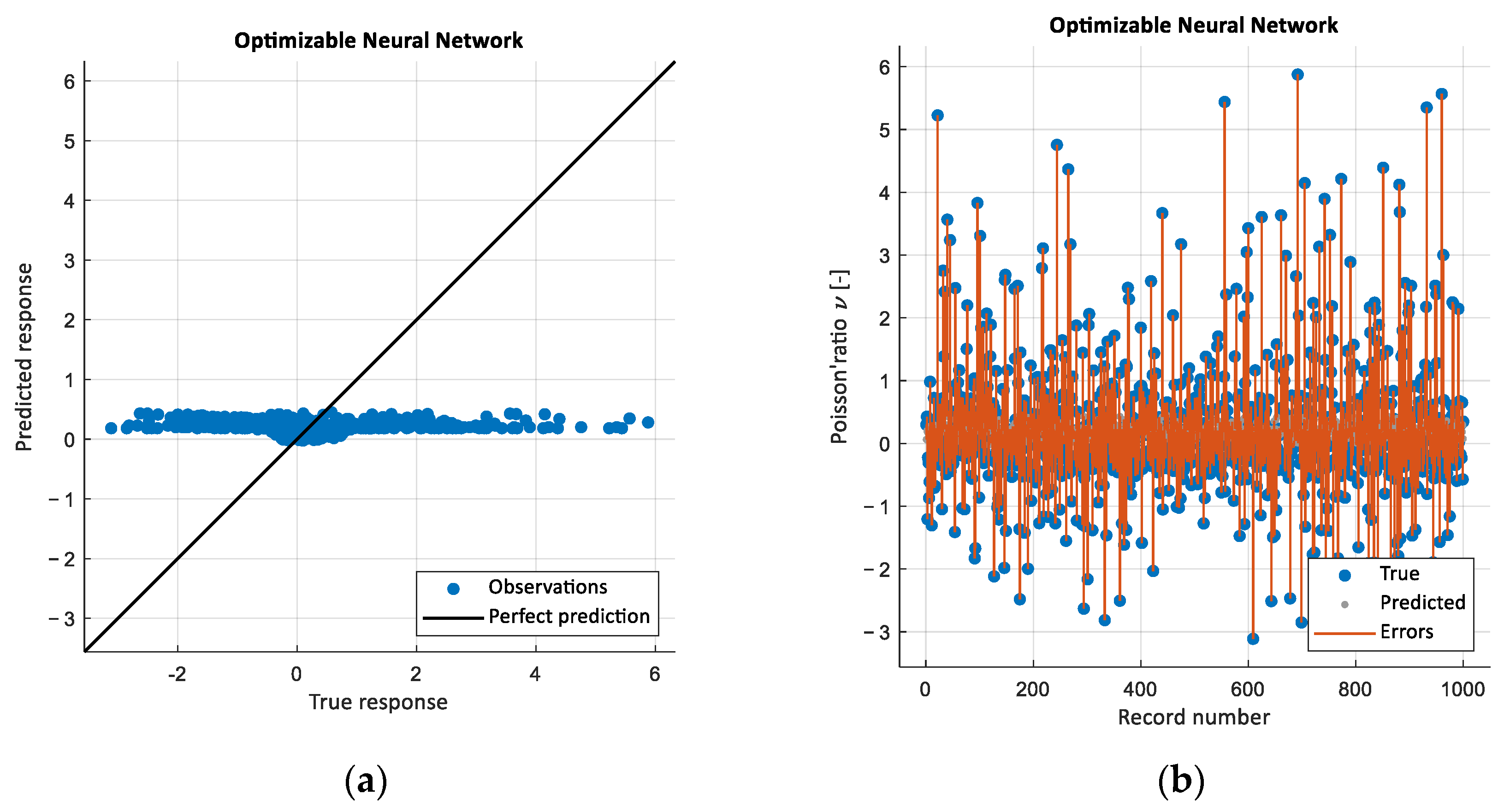
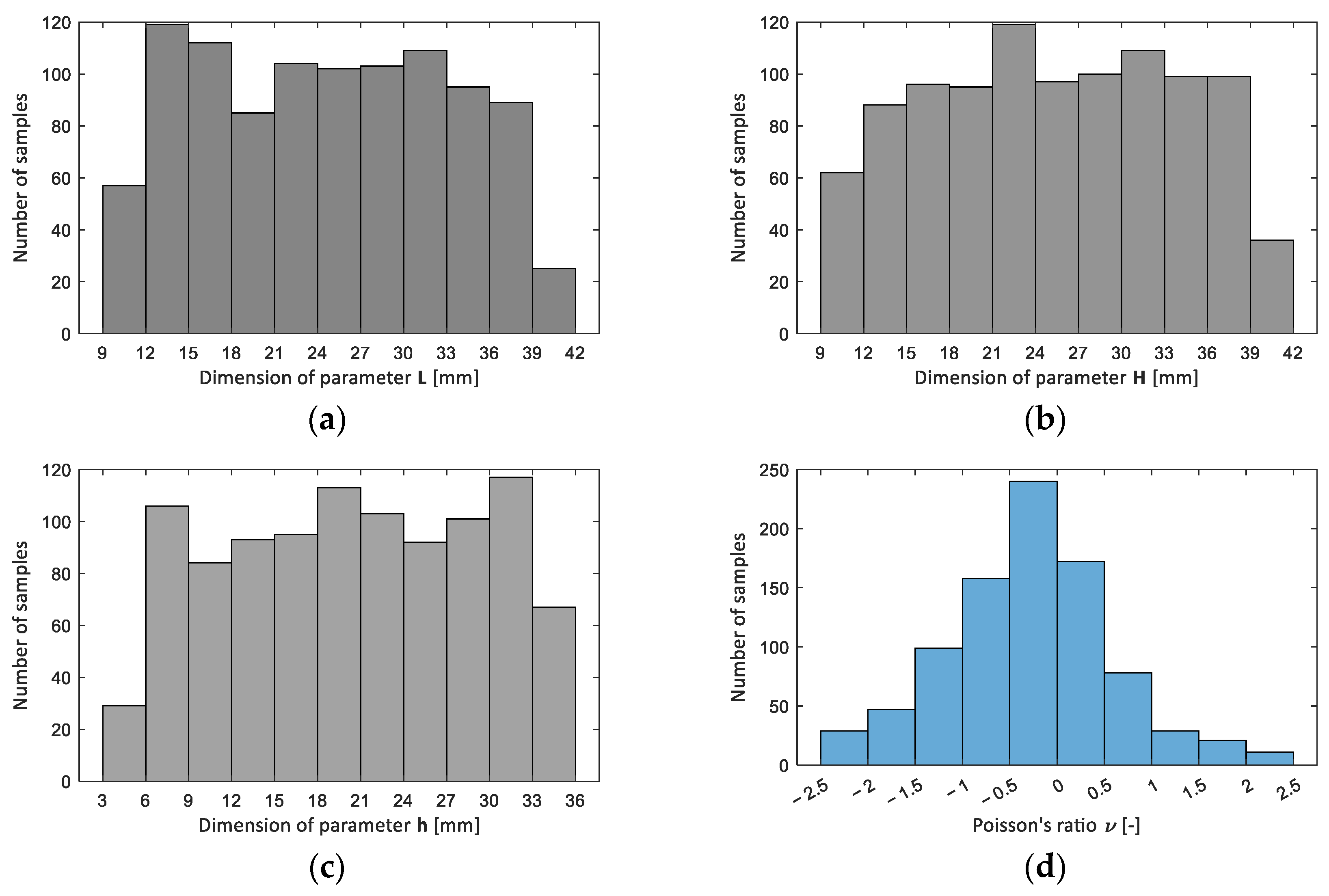
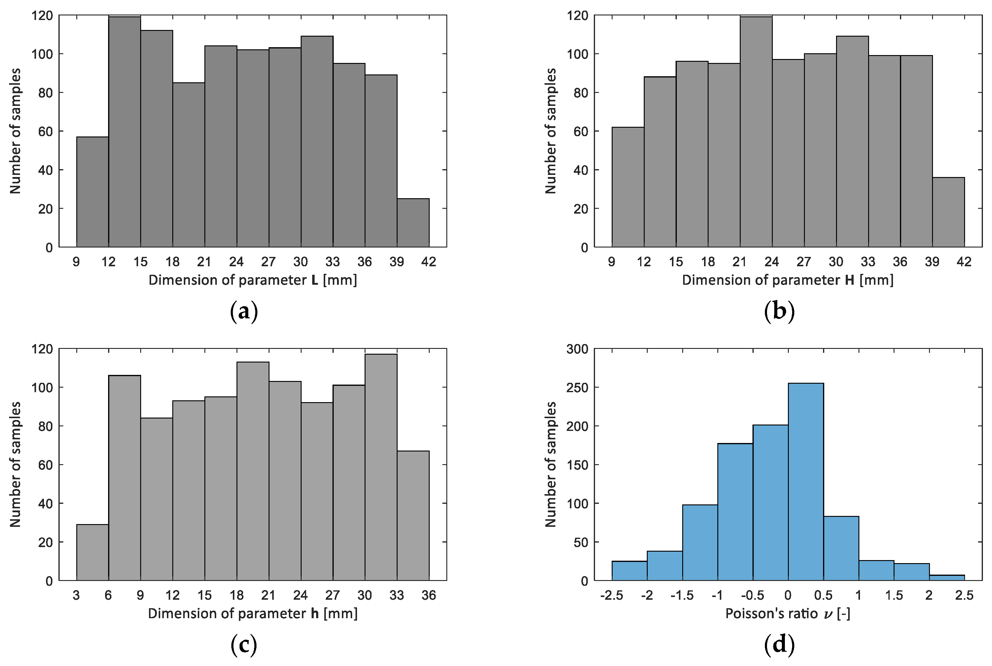
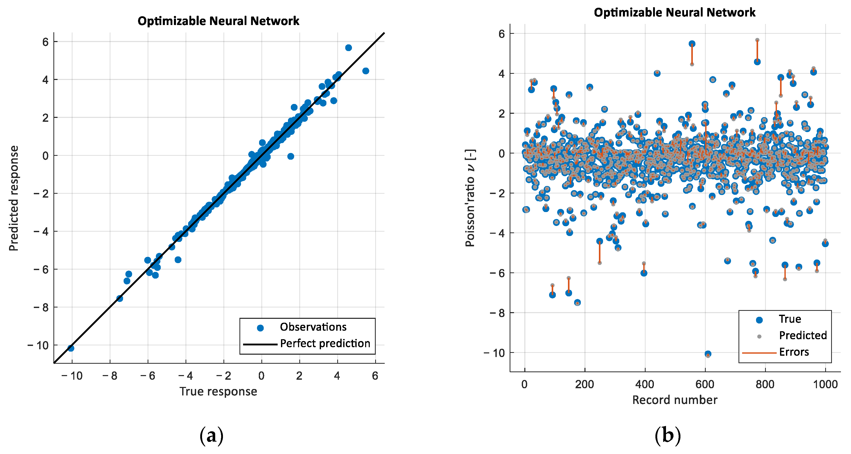
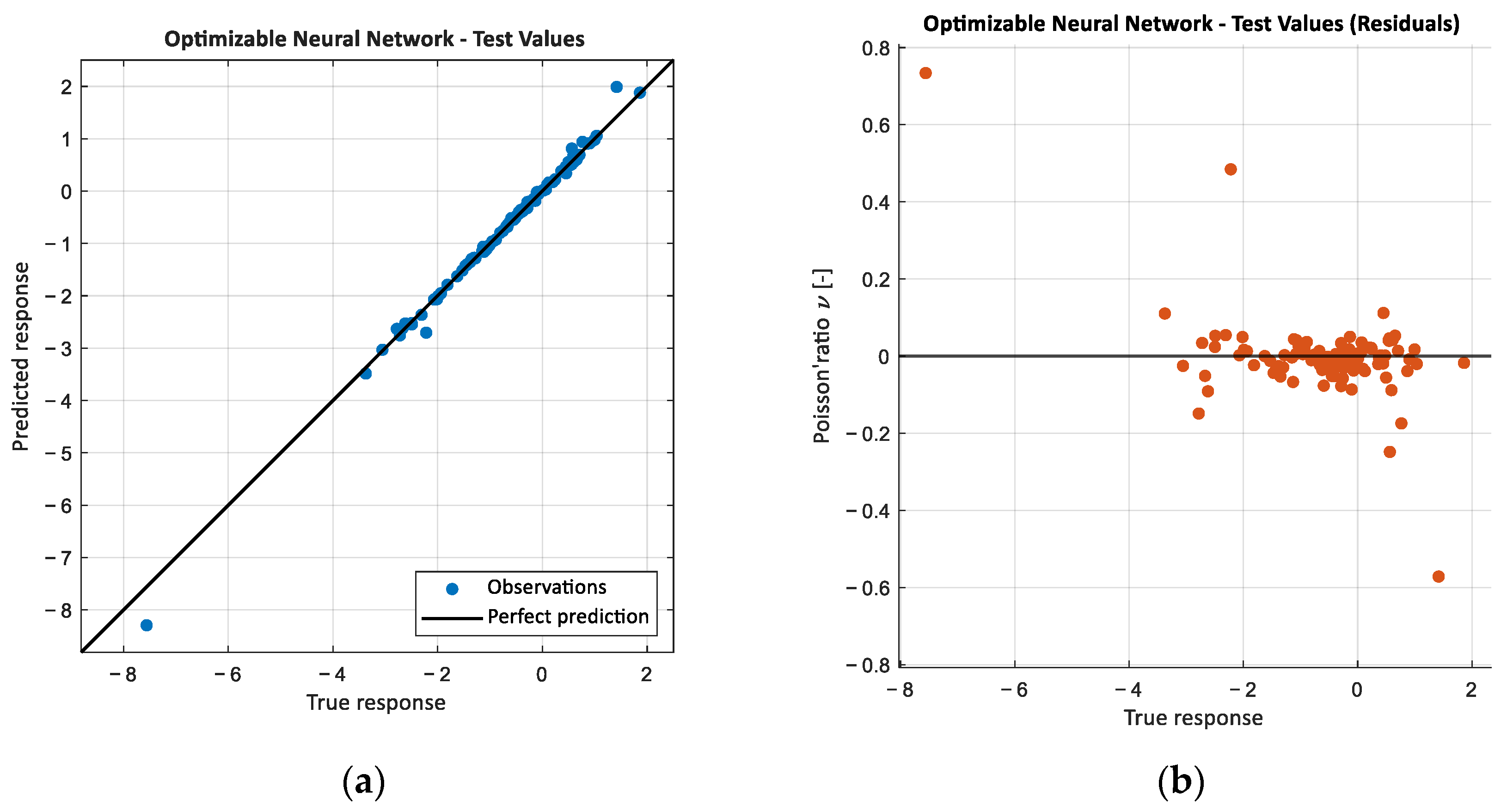
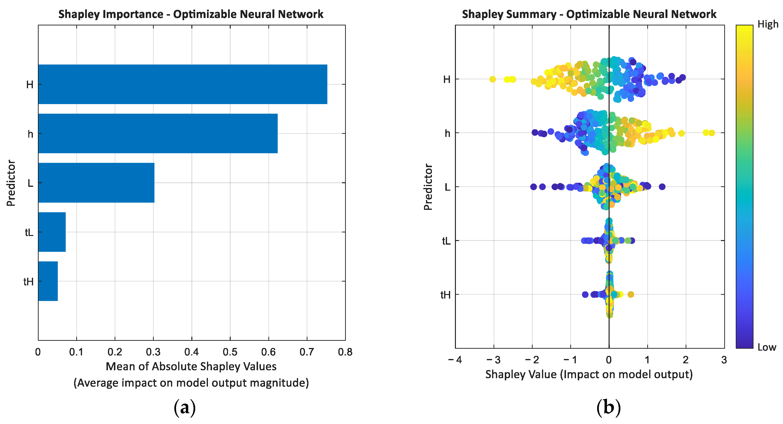
4.3. Machine Learning—Regression Learner

Although the structure was widely investigated, several analytical solutions and numerical results are reported. A question was raised to see if using existing results for training models to provide results for Poisson’s ratio is possible [22,56].

The parametric analysis discussed above can provide an overview of the selection method for the dimensional parameters.

The numerical model was used to generate data considering the variation of several parameters. Each set contains $1000$ lines. The values were randomly generated in the interval $\left[10\dots 40\right]$ for the ligaments and $\left[1\dots 3\right]$ for the thicknesses.

Input data is used to train MATLAB neural networks for regression analysis. The selected type was neural network with Bayesian optimization. The number of parameters ranges from two to five.

Table 3. Regression analysis—optimizable neural networks. Performance indicators.

Model (p)	$\mathit{R}\mathit{M}\mathit{S}\mathit{E}$	${\mathit{R}}^2$
2	1.0769	0.006
2 + 1	0.0427	0.9984
3	0.0642	0.9987
5	0.1300	0.9902
5-2	0.3867	0.9135

lists the performance indicators of the neural models, providing an overview of methods for designing honeycomb structures as a function of the input parameters $\left(p\right)$.

The first analysis was performed using a minimal number of parameters: length of horizontal ligament $L$ and the length of the vertical ligament $H$. Figure 14a,b present the statistical analysis of the input parameters, while Figure 14d presents the value of Poisson’s ratio as obtained from the numerical simulation.

Figure 15a presents the predicted response after training the neural model. Figure 15b presents the actual, predicted, and errors obtained using this model.

The results reported in Figure 16 show a significant deviation of the predicted response from the true response, which indicates that insufficient data were used for the analysis.

Comparing the input results with the analytical solution proposed by Gibson et al. [2] a third parameter was added to the input dataset as the computed angle $\theta$. Results obtained from the regression analysis are presented in Figure 14.

The model can provide accurate results for input datasets. A second input dataset with 1000 recordings was constructed using the numerical model. Statistical data are presented in Figure 17.

The results obtained using the regression model are presented in Figure 18.

The results are accurate as the input data $\left(L,H,h\right)$ for this dataset, the sets are similar in construction to the previous augmented set $\left(L,H,\theta \right)$.

The third input dataset with 1000 recordings was constructed using the numerical model and all dimensional parameters $\left(L,H,h,t_L,t_H\right)$. Statistical data are presented in Figure 19.

Figure 20 presents the results obtained using the regression model. Although the number of inputs is complex, the model can accurately estimate the structure’s behavior.

As demonstrated by the results, two parameters are not sufficient for the investigation of the structure. Adding a third parameter is capable of defining precision models with coefficients of determination higher than $0.998$. The use of a complete set of parameters is also feasible. The coefficient of determination is higher than $0.99$.

A scenario can be configured to evaluate the neural networks trained with incomplete data sets. This is the case when partial entries from the third dataset are used. The data corresponding to the thickness of the ligaments $\left(t_L, t_H\right)$ were removed. The results provided by the neural model are presented in Figure 21.

The data reveal that for machine learning processes, the input data must be consistent with the method used to generate results; otherwise, significant errors that alter the predictive performance of programmed models are generated.

An additional dataset with 100 records was created to test the learning model. Dataset statistics are presented in Figure 22. It can be noticed that the values follow the pattern given in Figure 19, with most of the data points within the interval $-0.5\dots 0.5$.

The model performance is displayed in Figure 23a as a comparison between observations and perfect predictions. The coefficient of determination displays a value $R^2=0.99149$ while the root mean square error decreases to $RMSE=0.11623$, proving the capacity of developing a performant model using the training dataset provided, using as a justification the majority of the values determined for the residuals $\left(∆\nu =-0.2\dots 0.2\right)$.

MATLAB provides a tool for evaluating the performance of a regression analysis model. The Shapley values of the predictors (Figure 24) provide a view of their importance over the model output magnitude.

Results presented in Figure 24a reveal that for a five-parameter model, the most important parameters are the dimension of the vertical ligament $\left(H\right)$, followed by the inner gap $\left(h\right)$. These parameters define the shape of the unit cell—from honeycomb with positive Poisson’s ratio to re-entrant with negative Poisson’s ratio. The data presented in Figure 24b provides a detailed view of the impact of the parameter on each predicted result. As expected, increasing the dimension of the horizontal ligament for a given value of the inner gap will increase the negative ratio behavior. The dimension of the vertical ligament and the inner gap are strongly connected. The following parameter, which drives and influences the behavior of the unit cell, is the length of the horizontal ligament; however, this parameter is strongly connected, closely tied to the definition of the vertical ligament and the inner gap. The thicknesses of the ligaments define a secondary set that can be used to adjust the mechanical behavior of the cell.

5. Conclusions

The results demonstrate the mechanical performance of the honeycomb structures in terms of deformation behaviour under axial loads. The problem was addressed considering the existing theoretical models and numerical simulations. Although based on a simplified formulation (Bernoulli model), the models are capable of producing reliable results by investigating the meshing method.

The honeycomb cell is simple in terms of geometric definition; however, when a series of parameters is investigated, it raises a range of questions regarding its behavior.

The convergence analysis provided a solution for the meshing method, and analyzing the results enabled the definition of an empirical solution that connects the unit cell to the structure.

The parametric analysis allowed the investigation of the influence of dimensions to determine the most efficient design approach.

Nowadays, machine learning is a game-changer in many areas, and engineering is one of the targets. Large datasets with one thousand entries were generated and used to train regression models. The required number of parameters to be defined was investigated. Evaluations were conducted to assess the predictions of the neural models using partial datasets.

The results demonstrate that integrating numerical methods with machine learning techniques can optimize the design of auxetic structures, significantly reducing computational effort. Extending this study to other auxetic geometries and advanced materials, such as shape-memory composites, could open new applications in mechanical and biomedical engineering.

Ultimately, the present study can serve as a reference for when relatively simple numerical methods are employed to analyze complex structures.

References

1. Xue, X.; Lin, C.; Wu, F.; Li, Z.; Liao, J. Lattice Structures with Negative Poisson’s Ratio: A Review. Mater. Today Commun. 2023, 34, 105132. [Google Scholar] [CrossRef]
2. Gibson, L.J.; Schajer, M.F.; Schajerj, J.G.S. The Mechanics of Two-Dimensional Cellular Materials. R. Soc. 1982, 382, 25–42. [Google Scholar]
3. Stronge, W.J.; Shim, P.-W. Dynamic Crushing of a Ductile Cellular Array. Int. J. Mech. Sci. 1987, 29, 381–406. [Google Scholar] [CrossRef]
4. Banhart, J. Manufacture, Characterisation and Application of Cellular Metals and Metal Foams. Prog. Mater. Sci. 2001, 46, 559–632. [Google Scholar] [CrossRef]
5. Lakes, R. Cellular Solid Structures with Unbounded Thermal Expansion. J. Mater. Sci. Lett. 1996, 15, 477. [Google Scholar] [CrossRef]
6. Jiao, P. Mechanical Energy Metamaterials in Interstellar Travel. Prog. Mater. Sci. 2023, 137, 101132. [Google Scholar] [CrossRef]
7. Li, X.; Peng, W.; Wu, W.; Xiong, J.; Lu, Y. Auxetic Mechanical Metamaterials: From Soft to Stiff. Int. J. Extrem. Manuf. 2023, 5, 042003. [Google Scholar] [CrossRef]
8. Sanami, M.; Ravirala, N.; Alderson, K.; Alderson, A. Auxetic Materials for Sports Applications. In Proceedings of the Procedia Engineering; Elsevier Ltd.: Amsterdam, The Netherlands, 2014; Volume 72, pp. 453–458. [Google Scholar]
9. Tan, X.; Chen, X. Parameters Affecting Energy Absorption and Deformation in Textile Composite Cellular Structures. Mater. Des. 2005, 26, 424–438. [Google Scholar] [CrossRef]
10. Kier, Z.T.; Salvi, A.; Theis, G.; Waas, A.M.; Shahwan, K. Estimating Mechanical Properties of 2D Triaxially Braided Textile Composites Based on Microstructure Properties. Compos. Part B Eng. 2015, 68, 288–299. [Google Scholar] [CrossRef]
11. Wang, H.; Zhang, C.; Wang, C.; Qiu, J. The Application of Negative Poisson’s Ratio Metamaterials in the Optimization of a Variable Area Wing. Aerospace 2025, 12, 125. [Google Scholar] [CrossRef]
12. Thompson, M.K.; Moroni, G.; Vaneker, T.; Fadel, G.; Campbell, R.I.; Gibson, I.; Bernard, A.; Schulz, J.; Graf, P.; Ahuja, B.; et al. Design for Additive Manufacturing: Trends, Opportunities, Considerations, and Constraints. CIRP Ann. Manuf. Technol. 2016, 65, 737–760. [Google Scholar] [CrossRef]
13. Rao, R.V.; Rai, D.P. Optimization of Fused Deposition Modeling Process Using Teaching-Learning-Based Optimization Algorithm. Eng. Sci. Technol. Int. J. 2016, 19, 587–603. [Google Scholar] [CrossRef]
14. Zadpoor, A.A. Mechanical Performance of Additively Manufactured Meta-Biomaterials. Acta Biomater. 2019, 85, 41–59. [Google Scholar] [CrossRef] [PubMed]
15. du Plessis, A.; Razavi, S.M.J.; Benedetti, M.; Murchio, S.; Leary, M.; Watson, M.; Bhate, D.; Berto, F. Properties and Applications of Additively Manufactured Metallic Cellular Materials: A Review. Prog. Mater. Sci. 2022, 125, 100918. [Google Scholar] [CrossRef]
16. Kelkar, P.U.; Kim, H.S.; Cho, K.H.; Kwak, J.Y.; Kang, C.Y.; Song, H.C. Cellular Auxetic Structures for Mechanical Metamaterials: A Review. Sensors 2020, 20, 3132. [Google Scholar] [CrossRef]
17. Dong, H.; Wang, H.; Hazell, P.J.; Sun, N.; Dura, H.B.; Escobedo-Diaz, J.P. Effects of Printing Parameters on the Quasi-Static and Dynamic Compression Behaviour of 3D-Printed Re-Entrant Auxetic Structures. Thin-Walled Struct. 2025, 210, 113000. [Google Scholar] [CrossRef]
18. Tian, Z.; Shi, S.; Liao, Y.; Wang, W.; Zhang, L.; Xiao, Y. Energy Absorption Mechanisms of Riveted and Assembled Double-Trapezoidal Auxetic Honeycomb Core Structures Under Quasi-Static Loading. J. Compos. Sci. 2025, 9, 89. [Google Scholar] [CrossRef]
19. Széles, L.; Horváth, R.; Cveticanin, L. Research on Auxetic Lattice Structure for Impact Absorption in Machines and Mechanisms. Mathematics 2024, 12, 1983. [Google Scholar] [CrossRef]
20. Chen, Z.; Wu, X.; Xie, Y.M.; Wang, Z.; Zhou, S. Re-Entrant Auxetic Lattices with Enhanced Stiffness: A Numerical Study. Int. J. Mech. Sci. 2020, 178, 105619. [Google Scholar] [CrossRef]
21. Panowicz, R.; Jeschke, A.; Durejko, T.; Zachman, M.; Konarzewski, M. The Mechanical Properties and Energy Absorption of AuxHex Structures. Materials 2024, 17, 6073. [Google Scholar] [CrossRef]
22. Peng, X.; Zhou, K.; Han, Y.; Jia, W.; Li, J.; Jiang, S. Compression Performance Analysis of Hexagonal and Re-Entrant Hybrid Honeycomb Structures. Polym. Test. 2025, 145, 108745. [Google Scholar] [CrossRef]
23. Zhang, X.; An, C.; Shen, Z.; Wu, H.; Yang, W.; Bai, J. Dynamic Crushing Responses of Bio-Inspired Re-Entrant Auxetic Honeycombs under in-Plane Impact Loading. Mater. Today Commun. 2020, 23, 100918. [Google Scholar] [CrossRef]
24. Liu, Y.; Schaedler, T.A.; Jacobsen, A.J.; Chen, X. Quasi-Static Energy Absorption of Hollow Microlattice Structures. Compos. Part B Eng. 2014, 67, 39–49. [Google Scholar] [CrossRef]
25. Mohsenizadeh, S.; Alipour, R.; Shokri Rad, M.; Farokhi Nejad, A.; Ahmad, Z. Crashworthiness Assessment of Auxetic Foam-Filled Tube under Quasi-Static Axial Loading. Mater. Des. 2015, 88, 258–268. [Google Scholar] [CrossRef]
26. Hong, S.T.; Pan, J.; Tyan, T.; Prasad, P. Quasi-Static Crush Behavior of Aluminum Honeycomb Specimens under Compression Dominant Combined Loads. Int. J. Plast. 2006, 22, 73–109. [Google Scholar] [CrossRef]
27. Qi, C.; Jiang, F.; Yang, S.; Remennikov, A. Multi-Scale Characterization of Novel Re-Entrant Circular Auxetic Honeycombs under Quasi-Static Crushing. Thin-Walled Struct. 2021, 169, 108314. [Google Scholar] [CrossRef]
28. Lu, H.; Wang, X.; Chen, T. In-Plane Dynamics Crushing of a Combined Auxetic Honeycomb with Negative Poisson’s Ratio and Enhanced Energy Absorption. Thin-Walled Struct. 2021, 160, 107366. [Google Scholar] [CrossRef]
29. Sun, Y.; Li, Q.M. Dynamic Compressive Behaviour of Cellular Materials: A Review of Phenomenon, Mechanism and Modelling. Int. J. Impact Eng. 2018, 112, 74–115. [Google Scholar] [CrossRef]
30. Ma, Q.; Zhang, J. Nonlinear Constitutive and Mechanical Properties of an Auxetic Honeycomb Structure. Mathematics 2023, 11, 2062. [Google Scholar] [CrossRef]
31. Ai, L.; Gao, X.L. An Analytical Model for Star-Shaped Re-Entrant Lattice Structures with the Orthotropic Symmetry and Negative Poisson’s Ratios. Int. J. Mech. Sci. 2018, 145, 158–170. [Google Scholar] [CrossRef]
32. Jiang, F.; Yang, S.; Qi, C. Quasi-Static Crushing Response of a Novel 3D Re-Entrant Circular Auxetic Metamaterial. Compos. Struct. 2022, 300, 116066. [Google Scholar] [CrossRef]
33. Luo, H.; Gao, Q.; Zhou, J.; Zhang, Y.; Bao, F.; Chen, J.; Cui, Y.; Wang, L.; Wang, X. Hybrid Honeycombs with Re-Entrant Auxetic and Face-Centered Cubic Cells: Design and Mechanical Characteristics. Eng. Struct. 2025, 328, 119731. [Google Scholar] [CrossRef]
34. Bora, K.M.; Varshney, S.K.; Kumar, C.S. Rounded Corner Thicken Strut Re-Entrant Auxetic Honeycomb: Analytical and Numerical Modeling. Mech. Res. Commun. 2024, 136, 104246. [Google Scholar] [CrossRef]
35. Zhang, W.; Zhao, S.; Scarpa, F.; Wang, J.; Sun, R. In-Plane Mechanical Behavior of Novel Auxetic Hybrid Metamaterials. Thin-Walled Struct. 2021, 159, 107191. [Google Scholar] [CrossRef]
36. Jiang, Y.; Rudra, B.; Shim, J.; Li, Y. Limiting Strain for Auxeticity under Large Compressive Deformation: Chiral vs. Re-Entrant Cellular Solids. Int. J. Solids Struct. 2019, 162, 87–95. [Google Scholar] [CrossRef]
37. Schürger, B.; Pástor, M.; Frankovský, P.; Lengvarský, P. Photoelasticity as a Tool for Stress Analysis of Re-Entrant Auxetic Structures. Appl. Sci. 2025, 15, 1250. [Google Scholar] [CrossRef]
38. Liu, X.; Shapiro, V. Homogenization of Material Properties in Additively Manufactured Structures. Comput.-Aided Des. 2016, 78, 71–82. [Google Scholar] [CrossRef]
39. Wang, T.; Wang, L.; Ma, Z.; Hulbert, G.M. Elastic Analysis of Auxetic Cellular Structure Consisting of Re-Entrant Hexagonal Cells Using a Strain-Based Expansion Homogenization Method. Mater. Des. 2018, 160, 284–293. [Google Scholar] [CrossRef]
40. Gunaydin, K.; Gülcan, O.; Tamer, A. Application of Homogenization Method in Free Vibration of Multi-Material Auxetic Metamaterials. Vibration 2025, 8, 2. [Google Scholar] [CrossRef]
41. Gongora, A.E.; Snapp, K.L.; Pang, R.; Tiano, T.M.; Reyes, K.G.; Whiting, E.; Lawton, T.J.; Morgan, E.F.; Brown, K.A. Designing Lattices for Impact Protection Using Transfer Learning. Matter 2022, 5, 2829–2846. [Google Scholar] [CrossRef]
42. Hasanzadeh, R. A New Polymeric Hybrid Auxetic Structure Additively Manufactured by Fused Filament Fabrication 3D Printing: Machine Learning-Based Energy Absorption Prediction and Optimization. Polymers 2024, 16, 3565. [Google Scholar] [CrossRef] [PubMed]
43. Al-Rifaie, H.; Movahedi, N.; Lim, T.C. Development of Novel Auxetic-Nonauxetic Hybrid Metamaterial. Eng. Fail. Anal. 2025, 175, 109559. [Google Scholar] [CrossRef]
44. Masters, I.G.; Evans, K.E. Models for the Elastic Deformation of Honeycombs. Compos. Struct. 1996, 35, 403–422. [Google Scholar] [CrossRef]
45. Grima, J.N.; Attard, D.; Ellul, B.; Gatt, R. An Improved Analytical Model for the Elastic Constants of Auxetic and Conventional Hexagonal Honeycombs. Cell. Polym. 2011, 30, 287–310. [Google Scholar] [CrossRef]
46. Tabacu, S.; Negrea, R.F.; Negrea, D. Experimental, Numerical and Analytical Investigation of 2D Tetra-Anti-Chiral Structure under Compressive Loads. Thin-Walled Struct. 2020, 155, 106929. [Google Scholar] [CrossRef]
47. Rao, S.S. The Finite Element Method in Engineering; Elsevier Butterworth-Heinmann: Oxford, UK, 2005; ISBN 0-7506-7828-3. [Google Scholar]
48. Wang, G.; Qi, Z.; Xu, J. A High-Precision Co-Rotational Formulation of 3D Beam Elements for Dynamic Analysis of Flexible Multibody Systems. Comput. Methods Appl. Mech. Eng. 2020, 360, 112701. [Google Scholar] [CrossRef]
49. Khakalo, S.; Balobanov, V.; Niiranen, J. Modelling Size-Dependent Bending, Buckling and Vibrations of 2D Triangular Lattices by Strain Gradient Elasticity Models: Applications to Sandwich Beams and Auxetics. Int. J. Eng. Sci. 2018, 127, 33–52. [Google Scholar] [CrossRef]
50. Günaydın, K.; Rea, C.; Kazancı, Z. Energy Absorption Enhancement of Additively Manufactured Hexagonal and Re-Entrant (Auxetic) Lattice Structures by Using Multi-Material Reinforcements. Addit. Manuf. 2022, 59, 103076. [Google Scholar] [CrossRef]
51. Surjadi, J.U.; Gao, L.; Du, H.; Li, X.; Xiong, X.; Fang, N.X.; Lu, Y. Mechanical Metamaterials and Their Engineering Applications. Adv. Eng. Mater. 2019, 21, 1800864. [Google Scholar] [CrossRef]
52. Yang, J.; Bhattacharya, K. Augmented Lagrangian Digital Image Correlation. Exp. Mech. 2019, 59, 187–205. [Google Scholar] [CrossRef]
53. Popławski, A.; Bogusz, P.; Grudnik, M. Digital Image Correlation and Numerical Analysis of Mechanical Behavior in Photopolymer Resin Lattice Structures. Materials 2025, 18, 384. [Google Scholar] [CrossRef] [PubMed]
54. Tabacu, S.; Predoiu, P.; Negrea, R. A Theoretical Model for the Estimate of Plateau Force for the Crushing Process of 3D Auxetic Anti-Tetra Chiral Structures. Int. J. Mech. Sci. 2021, 199, 106405. [Google Scholar] [CrossRef]
55. Zhang, X.G.; Ren, X.; Jiang, W.; Zhang, X.Y.; Luo, C.; Zhang, Y.; Xie, Y.M. A Novel Auxetic Chiral Lattice Composite: Experimental and Numerical Study. Compos. Struct. 2022, 282, 115043. [Google Scholar] [CrossRef]
56. Sinha, P.; Mukhopadhyay, T. Programmable Multi-Physical Mechanics of Mechanical Metamaterials. Mater. Sci. Eng. R Rep. 2023, 155, 100745. [Google Scholar] [CrossRef]
Figure 1. The cell: (a) conventional honeycomb cell; (b) re-entrant auxetic configuration. Note: The parameters are adapted to the context of the current work.
Mathematics 13 01676 g001
Figure 2. Definition of the numerical model: (a) quarter model of the structure (geometrical feature); (b) complete geometrical model (mirror operations about horizontal and vertical axes); (c) nodes seeds for the geometrical features; (d) definition of the beams; (e) complete model; (f) definition of the tracked nodes for the evaluation of Poisson’s ratio; (g) part definition; (h) loading conditions.
Mathematics 13 01676 g002
Figure 3. Definition of the numerical beam sizes: (a) uniform spacing r e = 0 ; (b) progressive r e = 3 .
Mathematics 13 01676 g003
Figure 4. Convergence analysis: (a) equal spacing of the nodes along the geometrical support r e = 0 ; (b) progressive distribution of nodes r e = 3 ; L = 20   m m ; H = 20   m m ; h = 10   m m ; t = 1.0   m m ; w = 2.0   m m ; E 0 = 205   GPa ;   ν 0 = 0.3 .
Mathematics 13 01676 g004
Figure 5. Analytical vs. numerical solution.
Mathematics 13 01676 g005
Figure 6. Processing of digital images: (a) specimen L = 20   m m ; H = 20   m m ; h = 10   m m ; t = 1.2   m m ; w = 10.0   m m ; (b) selection of the region of interest; (c) binary image; (d) contour detection; (e) features recognition. Scale factor: s f = 0.159   m m / p x .
Mathematics 13 01676 g006
Figure 7. Relative displacement during the experiment.
Mathematics 13 01676 g007
Figure 8. Poisson’s ratio as a parameter of the number of stacked units: (a) unit value; (b) edge value; (c) averaged value.
Mathematics 13 01676 g008
Figure 9. Poisson’s ratio as a parameter of dimension L .
Mathematics 13 01676 g009
Figure 10. Poisson’s ratio as a parameter of dimension H .
Mathematics 13 01676 g010
Figure 11. Poisson’s ratio as a parameter of dimension h .
Mathematics 13 01676 g011
Figure 12. Poisson’s ratio as a parameter of dimension t L .
Mathematics 13 01676 g012
Figure 13. Poisson’s ratio as a parameter of dimension t H .
Mathematics 13 01676 g013
Figure 14. Input data for the neural model: (a) distribution of the values for the parameter L ; (b) distribution values for the parameter H ; (c) computed values for angle θ ; (d) computed values for Poisson’s ratio ν u .
Mathematics 13 01676 g014
Figure 15. Results of the regression analysis (2 parameters): (a) predicted response; (b) true vs. predicted response.
Mathematics 13 01676 g015
Figure 16. Results of the regression analysis (2 + 1 parameters): (a) predicted response; (b) true vs. predicted response.
Mathematics 13 01676 g016
Figure 17. Input data for the neural model (3 parameters): (a) distribution of the values for the parameter L ; (b) distribution values for the parameter H ; (c) distribution for parameter h ; (d) computed values for Poisson’s ratio ν u .
Mathematics 13 01676 g017
Figure 18. Results of the regression analysis (3 parameters): (a) predicted response; (b) true vs. predicted response.
Mathematics 13 01676 g018
Figure 19. Input data for the neural model (5 parameters): (a) distribution for the parameter L ; (b) distribution for the parameter H ; (c) distribution for parameter h ; (d) Poisson’s ratio ν u .
Mathematics 13 01676 g019
Figure 20. Results of the regression analysis (5 parameters): (a) predicted response; (b) true vs. predicted response.
Mathematics 13 01676 g020
Figure 21. Results of the regression analysis (5-2 parameters): (a) predicted response; (b) true vs. predicted response.
Mathematics 13 01676 g021
Figure 22. Test input data for the neural model (5 parameters): (a) distribution for the parameter L ; (b) distribution for the parameter H ; (c) distribution for parameter h ; (d) Poisson’s ratio ν u .
Mathematics 13 01676 g022
Figure 23. Test results of the regression analysis (5 parameters): (a) predicted response; (b) residuals.
Mathematics 13 01676 g023
Figure 24. Shapley analysis (5 parameters): (a) importance; (b) summary.
Mathematics 13 01676 g024