Fuzzy Clustering with Uninorm-Based Distance Measure

Abstract

In this paper, we suggest an algorithm of fuzzy clustering with a uninorm-based distance measure. The algorithm follows a general scheme of fuzzy c-means (FCM) clustering, but in contrast to the existing algorithm, it implements logical distance between data instances. The centers of the clusters calculated by the algorithm are less dispersed and are concentrated in the areas of the actual centers of the clusters that result in the more accurate recognition of the number of clusters and of data structure.

1. Introduction

In general, decision making starts with the formulation of possible alternatives, collecting required data, data analysis, the formulation of the decision criteria, and the choice of the alternatives based on the formulated criteria [1].

In simple cases of decision making with certain information and univariate data, the decision-making process is reduced to the choice of alternatives which minimize the payoff or maximize the reward. In cases of uncertain information, decision making is more complicated. It deals with the expected payoffs and rewards using probabilistic or other methods for handling uncertainty. Finally, in cases of multivariate data and multicriteria choices, decision making is hardly solvable by exact methods and can be considered a kind of art.

For example, in his book, Triantaphyllou [2] describes several methods of multicriteria decision making without suggesting any preferred technique. He indicates that each specific decision-making problem requires a specific method for its solution. Such an approach is supported by the authors of the book [3]. They stress “a growing need for methodologies that, on the basis of the ever-increasing wealth of data available, are able to take into account all the relevant points of view, technically called criteria, and all the actors involved” [3] (p. ix). Then, the authors present the classification of the methods for solving different decision-making problems.

To apply the methods of decision making, the raw data are preprocessed with the aim of recognizing possible patterns, and consequently, decreasing the number of instances, and, if possible, the number of dimensions [4]. The basic preprocessing procedure which decreases the number of instances used in the next steps of decision making is data classification [5,6], or, if any additional information is unavailable, data clustering [7,8].

The popular clustering method is the k-means algorithm, independently suggested by Lloyd [9] and by Forgy [10], and is known as the Lloyd–Forgy algorithm. This algorithm obtains $n$ instances and creates $k$ clusters, such that each instance is included into a single cluster for which Euclidean distance between the instance and the cluster’s center is minimal. The clusters are formed from the instances for which the within-cluster variances are also minimal. The FORTRAN implementation of the algorithm was published by Hartigan and Wong [11]. Currently, this algorithm is implemented in most statistical and mathematical software tools; for example, in MATLAB^®, it is implemented in the Statistics and Machine Learning Toolbox™ in the function kmeans [12].

The main disadvantage of the k-means algorithm and its direct successors is an inclusion of each instance only in a single cluster that often restricts the recognition of the data patterns and the interpretation of the obtained clusters.

To overcome this disadvantage, Bezdek [13,14] suggested the fuzzy clustering algorithm, which is widely known as the fuzzy c-means (FCM) algorithm. Following this algorithm, the clusters are considered fuzzy sets, and each instance is included in several clusters with certain degrees of membership. In its original version, the algorithm uses Euclidean distances between the instances and the degrees of membership are calculated based on these distances. The other versions of the algorithm follow its original structure but use the other distance measures. For example, the Fuzzy Logic Toolbox™ of MATLAB^® includes the function fcm [15], which implements the c-means algorithm with three distance measures: Euclidean distance, a distance measure based on the Mahalanobis distance from the instances and the cluster centers [16], and the exponential distance measure normalized by the probability of choosing the cluster [17]. For the overview of different versions of the c-means algorithm and the other fuzzy clustering methods, see the paper [18] and the book [19].

Along with the advantages of the fuzzy c-means clustering techniques, it inherits the following disadvantage of the k-means algorithm: both algorithms search for the predefined number of clusters and separate the cluster centers, even in cases where such separation does not follow from the data structures.

For example, if the data are a set of normally distributed instances, then it is expected that the clustering algorithm will recognize a single cluster, and the centers of all clusters will be placed close to the center of distribution. However, the c-means algorithm with the known distance measures does not provide such a result.

The suggested c-means algorithm with the uninorm-based distance solves this problem. Similarly to the other fuzzy c-means algorithms, the suggested algorithm has the same structure as original Bezdek algorithm; however, in contrast to the known methods, it considers the normalized instances as the truth values of certain propositions and implements fuzzy logical distance between them. The suggested distance is based on the probability-based uninorm and absorbing norm [20], which already demonstrated their usefulness in a wide range of decision-making and control tasks [21].

The suggested algorithm can be used for the recognition of the patterns in raw data and for data preprocessing in different decision-making problems.

The rest of the paper is organized as follows. In Section 2.1 we briefly outline the Bezdek fuzzy c-means algorithm, and in Section 2.2, we describe the uninorm and absorbing norm which will be used for the construction of the logical distance. Section 3 presents the main results: the distance measure based on the uninorm and absorbing norm (Section 3.1) and the resulting algorithm for fuzzy clustering (Section 3.2). In Section 3.3, we illustrate the activity of the algorithm by numerical simulations with different data distributions and compare the obtained results with the results provided by the known fuzzy c-means algorithms. Section 4 includes some discussable issues.

2. Materials and Methods

The suggested algorithm follows the structure of the Bezdek fuzzy c-means algorithm [13,14]; however, in contrast to the existing algorithms, it uses the logical distance based on the uninorm and absorbing norm [22,23]. Below, we briefly describe this algorithm and the used norms.

2.1. Fuzzy c-Means Algorithm

Assume that the raw data are given by the $d$-dimensional vectors of real numbers

$$X=\left(x_1,x_2,\dots ,x_n\right)\subset {\mathbb{R}}^d,$$

where $x_i=\left(x_{i1}, x_{i2},\dots ,x_{id}\right)$, $i=1, 2,\dots , n$, $n\ge 1$, $d\ge 1$ stands for the observation or instance of the data.

Given a number $m\le n$, denote by

$$Y=\left(y_1,y_2,\dots ,y_m\right)\subset {\mathbb{R}}^d$$

a vector of the cluster centers, where $y_j=\left(y_{j1}, y_{j2},\dots ,y_{jd}\right)$, $j=1, 2,\dots , m$, $m\ge 1$, $d\ge 1$, denotes the center of the $j$th cluster.

The problem is to define the centers $y_j$ of the clusters and to define the membership degree ${\mu }_{ij}\in \left[0, 1\right]$ of each instance $x_i$ to each cluster $j$.

The fuzzy c-means algorithm which solves this problem is outlined below in Algorithm 1 [13] (see also [14,15,17]).

Algorithm 1. Fuzzy c-means algorithm.

Input: $d$-dimensional data vectors $X=\left(x_1,x_2,\dots ,x_n\right)$, $n\ge 1$,    number of clusters $m$,    termination criterion $\epsilon \in \left(0, 1\right)$,    weighting exponent $q>1$,    function ${\mathrm{d}\mathrm{i}\mathrm{s}\mathrm{t}}^d$. Output: vector $Y=\left(y_1,y_2,\dots ,y_m\right)$, $m\ge 1$, of cluster centers,       matrix $\mathrm{M}=\left({\mu }_{ij}\right)$, $i=1, 2, \dots , n$, $j=1, 2,\dots , m$, of membership degrees.     Initialize the cluster centers $y_j$, $j=1, 2,\dots , m$, by random.     Initialize the membership degrees ${\mu }_{ij}$, $i=1, 2, \dots , n$, $j=1, 2,\dots , m$, $${\mu }_{ij}={\left({\displaystyle \frac{1}{{\mathrm{d}\mathrm{i}\mathrm{s}\mathrm{t}}^d\left(x_i,y_j\right)}}\right)}^{1/\left(q-1\right)}/{\sum }_{k=1}^m{\left({\displaystyle \frac{1}{{\mathrm{d}\mathrm{i}\mathrm{s}\mathrm{t}}^d\left(x_i,y_k\right)}}\right)}^{1/\left(q-1\right)}.$$     Do       Save membership degrees ${\mu }_{ij}^{\prime }={\mu }_{ij}$, $i=1, 2, \dots , n$, $j=1, 2,\dots , m$,       Calculate cluster centers $y_j={\sum }_{i=1}^n{\left({\mu }_{ij}\right)}^q{x}_i/{\sum }_{i=1}^n{\left({\mu }_{ij}\right)}^q$,       Calculate membership degrees $${\mu }_{ij}={\left({\displaystyle \frac{1}{{\mathrm{d}\mathrm{i}\mathrm{s}\mathrm{t}}^d\left(x_i,y_j\right)}}\right)}^{1/\left(q-1\right)}/{\sum }_{k=1}^m{\left({\displaystyle \frac{1}{{\mathrm{d}\mathrm{i}\mathrm{s}\mathrm{t}}^d\left(x_i,y_k\right)}}\right)}^{1/\left(q-1\right)},$$ ${\hspace{1em}\hspace{1em}\hspace{1em}\mathrm{w}\mathrm{h}\mathrm{e}\mathrm{r}\mathrm{e} \mathrm{d}\mathrm{i}\mathrm{s}\mathrm{t}}^d\left(x_i,y_j\right)$ is the distance between the instance $x_i$ and the cluster center $y_j$,     While ${\max }_{i,j}\left({\mu }_{ij}^{\prime }-{\mu }_{ij}\right)>\epsilon$.     Return $Y=\left(y_1,y_2,\dots ,y_m\right)$ and $\mathrm{M}=\left({\mu }_{ij}\right)$.

In the original version [13], the fuzzy c-means algorithm uses the Euclidean distance

$${\mathrm{d}\mathrm{i}\mathrm{s}\mathrm{t}}^d\left(x_i,y_j\right)=\sqrt{{\sum }_{l=1}^d{\left(x_{il}-y_{jl}\right)}^2},$$

and in the succeeding versions [16,17], and the other distance measures were applied.

In this paper, we suggest using the logical distance measure based on the uninorm and absorbing norm which results in the more accurate recognition of the cluster centers.

2.2. Uninorm and Absorbing Norm

Uninorm [22] and absorbing norm [23] are the operators of fuzzy logic which extend Boolean operators and are used for aggregating truth values.

Uninorm aggregator ${\oplus }_{\theta }$ with the neutral element $\theta \in \left[0,1\right]$ is a function ${⨁}_{\theta }:\left[0,1\right]\times \left[0,1\right]\to \left[0,1\right]$ satisfying the following properties [22]; $x,y,z\in \left[0,1\right]$:

a. Commutativity:  $x{\oplus }_{\theta }y=y{\oplus }_{\theta }x$,

b. Associativity:         $\left(x{\oplus }_{\theta }y\right){\oplus }_{\theta }z=x{\oplus }_{\theta }\left(y{\oplus }_{\theta }z\right)$,

c. Monotonicity:   $x\le y$ implies $x{\oplus }_{\theta }z\le y{\oplus }_{\theta }z$,

d. Identity:      $\theta {\oplus }_{\theta }x=x$ for some $\theta \in \left[0,1\right]$,

• and such that, if $\theta =1$, then $x{\oplus }_{1}y=x\wedge y$ is a conjunction operator and if $\theta =0$, then $x{\oplus }_{0}y=x\vee y$ is a disjunction operator.

An absorbing norm aggregator ${\otimes }_{\vartheta }$ with absorbing element $\vartheta \in \left[0,1\right]$ is a function ${\otimes }_{\vartheta }:\left[0,1\right]\times \left[0,1\right]\to \left[0,1\right]$ satisfying the following properties [23]; $x,y,z\in \left[0,1\right]$:

a. Commutativity:  $x{\otimes }_{\vartheta }y=y{\otimes }_{\vartheta }x$,

b. Associativity:         $\left(x{\otimes }_{\vartheta }y\right){\otimes }_{\vartheta }z=x{\otimes }_{\vartheta }\left(y{\otimes }_{\vartheta }z\right)$,

c. Absorbing element:  $\vartheta {\otimes }_{\vartheta }x=\vartheta$ for any $x\in \left[0,1\right]$.

• Operator ${\otimes }_{\vartheta }$ is a fuzzy analog of the negated $xor$ operator.

Let $u_{\theta }:\left(0,1\right)\to \left(-\mathrm{\infty },\mathrm{\infty }\right)$ and $v_{\vartheta }:\left(0,1\right)\to \left(-\mathrm{\infty },\mathrm{\infty }\right)$ be invertible, continuous, strictly monotonously increasing functions with the parameters $\theta ,\vartheta \in \left[0,1\right]$ such that

a. ${\lim }_{x\to 0}{u}_{\theta }\left(x\right)=-\mathrm{\infty }$,${\lim }_{x\to 0}{v}_{\vartheta }\left(x\right)=-\mathrm{\infty }$,

b. ${\lim }_{x\to 1}{u}_{\theta }\left(x\right)=+\mathrm{\infty }$, ${\lim }_{x\to 1}{v}_{\vartheta }\left(x\right)=+\mathrm{\infty }$,

c. $u_{\theta }\left(\theta \right)=\theta$, $v_{\vartheta }\left(\vartheta \right)=\vartheta$.

• Then, for any $x,y\in \left(0,1\right)$ hold [24]

  $$\begin{gathered} x{\oplus }_{\theta }y=u_{\theta }^{-1}\left(u_{\theta }\left(x\right)+u_{\theta }\left(y\right)\right), \\ x{\otimes }_{\vartheta }y=v_{\vartheta }^{-1}\left(v_{\vartheta }\left(x\right)\times v_{\vartheta }\left(y\right)\right), \end{gathered}$$

  and for the bounds $0$ and $1,$ the values of the operators ${\oplus }_{\theta }$ and ${\otimes }_{\vartheta }$ are defined in correspondence to the results of Boolean operators.

If $\theta =\vartheta$ and $u\equiv v$, then the interval $\left[0,1\right]$ with the operators ${\oplus }_{\theta }$ and ${\otimes }_{\vartheta }$ form the algebra [20,25]

$$\mathcal{A}=〈\left[0,1\right],{\oplus }_{\theta },{\otimes }_{\vartheta }〉$$

in which uninorm ${\oplus }_{\theta }$ acts as a summation operator and absorbing norm ${\otimes }_{\vartheta }$ acts as a multiplication operator. In this algebra, neutral element $\theta$ has a value of zero for the summation and absorbing element $\vartheta$ is a unit value for multiplication. Note that, in contrast to the algebra of real numbers, in the algebra $\mathcal{A}$, $\theta =\vartheta$ holds despite the different meanings of these values.

The inverse operators in this algebra are

$$\begin{gathered} x{\ominus }_{\theta }y=u_{\theta }^{-1}\left(u_{\theta }\left(x\right)-u_{\theta }\left(y\right)\right), x,y\in \left(0,1\right) \\ x{\oslash }_{\vartheta }y=v_{\vartheta }^{-1}\left(v_{\vartheta }\left(x\right)/v_{\vartheta }\left(y\right)\right), v\left(y\right)\ne 0. \end{gathered}$$

In addition, the negation operator is defined as

$${\ominus }_{\theta }x=u_{\theta }^{-1}\left(-u_{\theta }\left(x\right)\right), x\in \left(0,1\right).$$

In the paper [20], it was demonstrated that the functions $u_{\theta }$ and $v_{\vartheta }$ satisfy the requirements of quantile functions of probability distributions. Along with that, any function satisfying the indicated above requirements and its inverse are also applicable.

Here, we will assume that the functions $u_{\theta }\equiv v_{\vartheta }$ are equivalent. In the simulations, we will use the functions

$$u_{\theta }\left(x\right)=\ln {\displaystyle \frac{x^{\alpha }}{1-x^{\alpha }}}, x\in \left(0,1\right),$$

$$u_{\theta }^{-1}\left(\xi \right)={\left({\displaystyle \frac{e^{\xi }}{1+e^{\xi }}}\right)}^{1/\alpha }, \xi \in \left(-\mathrm{\infty },\mathrm{\infty }\right),$$

where $\alpha =1/{\log }_2{\displaystyle \frac{1}{\theta }}$, $\theta \in \left(0,1\right)$.

For other examples of the functions $u_{\theta }$ and $v_{\vartheta }$, see the paper [20] and the book [21].

3. Results

We start with the definition of logical distance based on the uninorm and absorbing norm, and then present the suggested algorithm. In the last subsection we consider numerical simulations and compare the suggested algorithm with the known method.

3.1. Logical Distance Based on the Uninorm and Absorbing Norm

Let $x,y\in \left[0,1\right]$ be two truth values. Given neutral element $\theta$ and absorbing element $\vartheta$, fuzzy logical dissimilarity of the values $x$ and $y$ is defined as follows:

$${\mathrm{d}\mathrm{i}\mathrm{s}\mathrm{i}\mathrm{m}}_{\theta ,\vartheta }\left(x,y\right)={\ominus }_{\theta }\left(\left(x{\oplus }_y\theta \right){\otimes }_{\vartheta }\left(\theta {\oplus }_{x}y\right)\right).$$

where the value

$${\mathrm{s}\mathrm{i}\mathrm{m}}_{\theta ,\vartheta }\left(x,y\right)=\left(x{\oplus }_y\theta \right){\otimes }_{\vartheta }\left(\theta {\oplus }_{x}y\right)$$

is a fuzzy logical similarity of the values $x$ and $y$.

If $\theta =\vartheta$, we will write ${\mathrm{d}\mathrm{i}\mathrm{s}\mathrm{i}\mathrm{m}}_{\theta }$ instead of ${\mathrm{d}\mathrm{i}\mathrm{s}\mathrm{i}\mathrm{m}}_{\theta ,\vartheta }$ and ${\mathrm{s}\mathrm{i}\mathrm{m}}_{\theta }$ instead of ${\mathrm{s}\mathrm{i}\mathrm{m}}_{\theta ,\vartheta }$.

Lemma 1.

If $\theta =\vartheta$, then the function ${disim}_{\theta }$is a semi-metric in the algebra $\mathcal{A}$.

Proof. 

To prove the lemma, we need to check the three following properties:

• ${\mathrm{d}\mathrm{i}\mathrm{s}\mathrm{i}\mathrm{m}}_{\theta ,\vartheta }\left(x,x\right)=\theta =\vartheta$.
  By the commutativity and identity properties of the uninorm holds

  $$x{\oplus }_x\theta =\theta {\oplus }_{x}x=\theta .$$
  Then, by the property of absorbing element holds

  $$\theta {\otimes }_{\theta }\theta =\theta$$

  and

  $${\ominus }_{\theta }\theta =\theta .$$
• ${\mathrm{d}\mathrm{i}\mathrm{s}\mathrm{i}\mathrm{m}}_{\theta ,\vartheta }\left(x,y\right)>\theta =\vartheta$ if $x\ne y$.
  If $x\ne y$, then either

  $$x{\oplus }_y\theta >\theta \mathrm{and} \theta {\oplus }_{x}y<\theta$$

  or

  $$x{\oplus }_y\theta <\theta \mathrm{and} \theta {\oplus }_{x}y>\theta .$$
  Thus,

  $$\left(x{\oplus }_y\theta \right){\otimes }_{\theta }\left(\theta {\oplus }_{x}y\right)<\theta$$

  and

  $${\ominus }_{\theta }\left(\left(x{\oplus }_y\theta \right){\otimes }_{\theta }\left(\theta {\oplus }_{x}y\right)\right)>\theta .$$
• ${\mathrm{d}\mathrm{i}\mathrm{s}\mathrm{i}\mathrm{m}}_{\theta ,\vartheta }\left(x,y\right)={\mathrm{d}\mathrm{i}\mathrm{s}\mathrm{i}\mathrm{m}}_{\theta ,\vartheta }\left(y,x\right)$.

It follows directly from the commutativity of the absorbing norm.

• Lemma is proven. □

Using the dissimilarity function, we define a fuzzy logical distance ${\mathrm{d}\mathrm{i}\mathrm{s}\mathrm{t}}_{\theta ,\vartheta }$ between the values $x,y\in \left[0,1\right]$ as follows ($\theta =\vartheta$):

$${\mathrm{d}\mathrm{i}\mathrm{s}\mathrm{t}}_{\theta ,\vartheta }\left(x,y\right)={\displaystyle \frac{1}{\theta }}{\mathrm{d}\mathrm{i}\mathrm{s}\mathrm{i}\mathrm{m}}_{\theta ,\vartheta }\left(x,y\right)-1.$$

Lemma 2.

If $\theta =\vartheta$, then the function ${dist}_{\theta }$is a semi-metric in the algebra of real numbers on the interval $\left[0, 1\right]$.

Proof. 

Since, for any $x,y\in \left[0,1\right]$ and any $\theta =\vartheta \in \left[0,1\right]$ both $x{\oplus }_{\theta }y\in \left[0,1\right]$, $x{\otimes }_{\vartheta }y\in \left[0,1\right]$ and ${\ominus }_{\theta }x\in \left[0,1\right]$, and by the properties a and b of semi-metric, holds

$${\mathrm{d}\mathrm{i}\mathrm{s}\mathrm{i}\mathrm{m}}_{\theta ,\vartheta }\left(x,y\right)\in \left[\theta ,1\right].$$

• If $x=y$, then ${\mathrm{d}\mathrm{i}\mathrm{s}\mathrm{i}\mathrm{m}}_{\theta ,\vartheta }\left(x,y\right)=\theta =\vartheta$ and
  $${\mathrm{d}\mathrm{i}\mathrm{s}\mathrm{t}}_{\theta ,\vartheta }\left(x,y\right)=0.$$
• If $x\ne y$, then ${\mathrm{d}\mathrm{i}\mathrm{s}\mathrm{i}\mathrm{m}}_{\theta ,\vartheta }\left(x,y\right)>\theta =\vartheta$. So ${\displaystyle \frac{1}{\theta }}{\mathrm{d}\mathrm{i}\mathrm{s}\mathrm{i}\mathrm{m}}_{\theta ,\vartheta }\left(x,y\right)>1$ and
  $${\mathrm{d}\mathrm{i}\mathrm{s}\mathrm{t}}_{\theta ,\vartheta }\left(x,y\right)>0.$$
• Symmetry

$${\mathrm{d}\mathrm{i}\mathrm{s}\mathrm{t}}_{\theta ,\vartheta }\left(x,y\right)={\mathrm{d}\mathrm{i}\mathrm{s}\mathrm{t}}_{\theta ,\vartheta }\left(y,x\right)$$

follows directly from the symmetry of the dissimilarity ${\mathrm{d}\mathrm{i}\mathrm{s}\mathrm{i}\mathrm{m}}_{\theta ,\vartheta }$. □

An example of the fuzzy logic distance ${\mathrm{d}\mathrm{i}\mathrm{s}\mathrm{t}}_{\theta ,\vartheta }\left(x,y\right)$ between the values $x,y\in \left[0,1\right]$ with $\theta =\vartheta =0.5$ is shown in Figure 1a. For comparison, Figure 1b shows the Euclidean distance between the values $x,y\in \left[0,1\right]$.

It is seen that the fuzzy logical distance better separates the close values and is less sensitive to the far values than Euclidean distance.

Now, let us extend the introduced fuzzy logical distance to multidimensional variables.

Let

$$\left(x_1,x_2,\dots ,x_n\right)\subset {\left[0, 1\right]}^d, n\ge 1, d\ge 1,$$

be $d$-dimensional vectors such that each vector $x_i=\left(x_{i1}, x_{i2},\dots ,x_{id}\right)$, $i=1, 2,\dots , n$, is a point in a $d$-dimensional space.

The fuzzy logical dissimilarity of the points $x_i$ and $x_j$, $i,j=1, 2,\dots , n$, is defined as follows:

$${\mathrm{d}\mathrm{i}\mathrm{s}\mathrm{i}\mathrm{m}}_{\theta ,\vartheta }^d\left(x_i,x_j\right)={\ominus }_{\theta }\left\{{{\oplus }_{\theta }}_{l=1}^d\left[\left(x_{il}{\oplus }_{x_{jl}}\theta \right){\otimes }_{\vartheta }\left(\theta {\oplus }_{x_{il}}{x}_{jl}\right)\right]\right\},$$

where, as above, the value

$${\mathrm{s}\mathrm{i}\mathrm{m}}_{\theta ,\vartheta }^d\left(x_i,x_j\right)={{\oplus }_{\theta }}_{l=1}^d\left[\left(x_{il}{\oplus }_{x_{jl}}\theta \right){\otimes }_{\vartheta }\left(\theta {\oplus }_{x_{il}}{x}_{jl}\right)\right]$$

is the fuzzy logical similarity of the points $x_i$ and $x_j$.

Let $\theta =\vartheta$. Then, as above, the fuzzy logical distance between the points $x_i$ and $x_j$, $i,j=1, 2,\dots , n$, is

$${\mathrm{d}\mathrm{i}\mathrm{s}\mathrm{t}}_{\theta ,\vartheta }^d\left(x_i,x_j\right)={\displaystyle \frac{1}{\theta }}{\mathrm{d}\mathrm{i}\mathrm{s}\mathrm{i}\mathrm{m}}_{\theta ,\vartheta }^d\left(x_i,x_j\right)-1.$$

Lemma 3.

If $\theta =\vartheta$, then the function ${disim}_{\theta }^d$is a semi-metric in the algebra $\mathcal{A}=〈{\left[0, 1\right]}^d, {\oplus }_{\theta }, {\otimes }_{\vartheta }〉$, $d\ge 1$.

Proof. 

This statement is a direct consequence of Lemma 1 and the properties of the uninorm.

• ${\mathrm{d}\mathrm{i}\mathrm{s}\mathrm{i}\mathrm{m}}_{\theta ,\vartheta }^d\left(x_i,x_j\right)=\theta =\vartheta$.
  If $x_i=x_j$, then for each $l=\mathrm{1,2},\dots ,d$

  $$\left(x_{il}{\oplus }_{x_{jl}}\theta \right){\otimes }_{\theta }\left(\theta {\oplus }_{x_{il}}{x}_{jl}\right)=\theta .$$
  Then,

  $${{\oplus }_{\theta }}_{l=1}^d\left[\left(x_{il}{\oplus }_{x_{jl}}\theta \right){\otimes }_{\vartheta }\left(\theta {\oplus }_{x_{il}}{x}_{jl}\right)\right]={{\oplus }_{\theta }}_{l=1}^d\theta =\theta$$

  and finally

  $${\ominus }_{\theta }\theta =\theta .$$
• ${\mathrm{d}\mathrm{i}\mathrm{s}\mathrm{i}\mathrm{m}}_{\theta ,\vartheta }^d\left(x_i,x_j\right)>\theta$ if $x\ne y$.
  If $x_i\ne x_j$, then for each $l=\mathrm{1,2},\dots ,d$

  $$\left(x_{il}{\oplus }_{x_{jl}}\theta \right){\otimes }_{\theta }\left(\theta {\oplus }_{x_{il}}{x}_{jl}\right)<\theta$$
  Then,

  $${{\oplus }_{\theta }}_{l=1}^d\left[\left(x_{il}{\oplus }_{x_{jl}}\theta \right){\otimes }_{\vartheta }\left(\theta {\oplus }_{x_{il}}{x}_{jl}\right)\right]<\theta$$

  and

  $${\ominus }_{\theta }\left\{{{\oplus }_{\theta }}_{l=1}^d\left[\left(x_{il}{\oplus }_{x_{jl}}\theta \right){\otimes }_{\vartheta }\left(\theta {\oplus }_{x_{il}}{x}_{jl}\right)\right]\right\}>\theta .$$
• ${\mathrm{d}\mathrm{i}\mathrm{s}\mathrm{i}\mathrm{m}}_{\theta ,\vartheta }^d\left(x_i,x_j\right)={\mathrm{d}\mathrm{i}\mathrm{s}\mathrm{i}\mathrm{m}}_{\theta ,\vartheta }^d\left(x_j,x_i\right)$.

It follows directly from the symmetry of dissimilarity for each $l=\mathrm{1,2},\dots ,d$ and the commutativity of the uninorm. □

Lemma 4.

If $\theta =\vartheta$, then the function ${dist}_{\theta ,\vartheta }^d$is a semi-metric on the hypercube ${\left[0, 1\right]}^d$, $d\ge 1$.

Proof. 

The proof is literally the same as the proof of Lemma 2. □

The suggested algorithm uses the introduced function ${\mathrm{d}\mathrm{i}\mathrm{s}\mathrm{t}}_{\theta ,\vartheta }^d$ as a distance measure between the instances of the data.

3.2. The c-Means Algorithm with Fuzzy Logical Distance

The suggested algorithm considers the instances of data as truth values and uses Algorithm 1 with fuzzy logical distance ${\mathrm{d}\mathrm{i}\mathrm{s}\mathrm{t}}_{\theta ,\vartheta }^d$ on these values.

As above, assume that the raw data are represented by $d$-dimensional vectors

$$X=\left(x_1,x_2,\dots ,x_n\right)\subset {\mathbb{R}}^d,$$

where $x_i=\left(x_{i1}, x_{i2},\dots ,x_{id}\right)$, $i=1, 2,\dots , n$, $n\ge 1$, $d\ge 1$, is a data instance.

Since function ${\mathrm{d}\mathrm{i}\mathrm{s}\mathrm{t}}_{\theta ,\vartheta }^d$ requires the values from the hypercube ${\left[0,1\right]}^d$, $\mathrm{d}\ge 1$, vector $X$ must be normalized

$$\tilde{X}=\mathrm{norm}\left(X\right), X\subset {\mathbb{R}}^d, \tilde{X}\subset {\left[0,1\right]}^d,$$

and the algorithm should be applied to the normalized data vector $\tilde{X}$. After the definition of the cluster centers $\tilde{Y}$, the inverse normalization must be applied to the vector $\tilde{Y}$

$$Y={\mathrm{norm}}^{-1}\left(\tilde{Y}\right), \tilde{Y}\subset {\left[0,1\right]}^d, Y\subset {\mathbb{R}}^d.$$

Normalization can be conducted by several methods; in Appendix A, we present a simple Algorithm A1 of normalization by linear transformation also called the min–max scaling. The inverse transformation provided by Algorithm A2 is also presented in Appendix A. These transformations are the simplest ones for the normalization of the raw data. Note that with respect to the task, other normalization methods can be applied.

In general, the suggested Algorithm 2 follows the Bezdek fuzzy c-means Algorithm 1, but differs in the distance function and in initialization of cluster centers ${\tilde{y}}_j$, $j=1, 2,\dots , m$, and, consequently, in the definition of the number of clusters.

Algorithm 2. Fuzzy c-means algorithm with fuzzy logical distance measure

Input: $d$-dimensional data vectors $X=\left(x_1,x_2,\dots ,x_n\right)\subset {\mathbb{R}}^d$, $n\ge 1$, $d\ge 1$,    termination criterion $\epsilon \in \left(0, 1\right)$,    weighting exponent $q>1$,    precision $\xi \in \left(0, 1\right)$,    distance function ${\mathrm{d}\mathrm{i}\mathrm{s}\mathrm{t}}_{\theta ,\vartheta }^d$ with the parameters $\theta ,\vartheta \in \left[0, 1\right]$. Output: vector $Y=\left(y_1,y_2,\dots ,y_m\right)$, $m\ge 1$, of cluster centers,       matrix $\mathrm{M}=\left({\mu }_{ij}\right)$, $i=1, 2, \dots , n$, $j=1, 2,\dots , m$, of membership degrees. Calculate normalized data vectors $\tilde{X}=\left({\tilde{x}}_1,{\tilde{x}}_2,\dots ,{\tilde{x}}_n\right)\subset {\left[0,1\right]}^d$ and the values $x_{min}$, ${\tilde{x}}_{max}$ using Algorithm A1. Initialize vector $\tilde{Y}=\left({\tilde{y}}_1,{\tilde{y}}_2,\dots ,{\tilde{y}}_m\right)\subset {\left[0,1\right]}^d$ of cluster centers as a $d$-dimensional grid with the step $\xi$ in the hypercube ${\left[0,1\right]}^d$. The number $m$ of clusters is defined as a number of nodes in this grid. Initialize the membership degrees $\hspace{1em}\hspace{1em}\hspace{1em}\hspace{1em}{\mu }_{ij}$, $i=1, 2, \dots , n$, $j=1, 2,\dots , m$, $${\mu }_{ij}={\left({\displaystyle \frac{1}{{\mathrm{d}\mathrm{i}\mathrm{s}\mathrm{t}}_{\theta ,\vartheta }^d\left({\tilde{x}}_i,{\tilde{y}}_j\right)}}\right)}^{1/\left(q-1\right)}/{\sum }_{k=1}^m{\left({\displaystyle \frac{1}{{\mathrm{d}\mathrm{i}\mathrm{s}\mathrm{t}}_{\theta ,\vartheta }^d\left({\tilde{x}}_i,{\tilde{y}}_k\right)}}\right)}^{1/\left(q-1\right)}.$$ Do    Save membership degrees ${\mu }_{ij}^{\prime }={\mu }_{ij}$, $i=1, 2, \dots , n$, $j=1, 2,\dots , m$,    Calculate cluster centers $${\tilde{y}}_j={\sum }_{i=1}^n{\left({\mu }_{ij}\right)}^q{\tilde{x}}_i/{\sum }_{i=1}^n{\left({\mu }_{ij}\right)}^q,$$    Calculate membership degrees $${\mu }_{ij}={\left({\displaystyle \frac{1}{{\mathrm{d}\mathrm{i}\mathrm{s}\mathrm{t}}_{\theta ,\vartheta }^d\left({\tilde{x}}_i,{\tilde{y}}_j\right)}}\right)}^{1/\left(q-1\right)}/{\sum }_{k=1}^m{\left({\displaystyle \frac{1}{{\mathrm{d}\mathrm{i}\mathrm{s}\mathrm{t}}_{\theta ,\vartheta }^d\left({\tilde{x}}_i,{\tilde{y}}_k\right)}}\right)}^{1/\left(q-1\right)},$$   where ${\mathrm{d}\mathrm{i}\mathrm{s}\mathrm{t}}_{\theta ,\vartheta }^d\left({\tilde{x}}_i,{\tilde{y}}_j\right)$ is the fuzzy logical distance between the instance ${\tilde{x}}_i$ and the cluster center ${\tilde{y}}_j$, While ${\max }_{i,j}\left({\tilde{\mu }}_{ij}-{\mu }_{ij}\right)>\epsilon$. Calculate renormalized vector $Y=\left(y_1,y_2,\dots ,y_m\right)\subset {\mathbb{R}}^d$ from the vector $\tilde{Y}=\left({\tilde{y}}_1,{\tilde{y}}_2,\dots ,{\tilde{y}}_m\right)\subset {\left[0,1\right]}^d$ using Algorithm A2. Return $Y=\left(y_1,y_2,\dots ,y_m\right)$ and $\mathrm{M}=\left({\mu }_{ij}\right)$.

The main difference between the suggested Algorithm 2 and the original Bezdek fuzzy c-means Algorithm 1 [13,14] and the known Gustafson–Kessel [16] and Gath–Geva [17] is the use of the fuzzy logical distance ${\mathrm{d}\mathrm{i}\mathrm{s}\mathrm{t}}_{\theta ,\vartheta }^d$. The use of this distance requires the normalization and renormalization of the data.

Another difference is in the need to initialize the cluster centers as a grid in the algorithm’s domain. Such initialization is required because of the quick convergence of the algorithm; thus, the regular distribution of initial cluster centers avoids missing clusters. A simple Algorithm A3 for creating a grid in the square ${\left[0,1\right]}^2$ is outlined in Appendix A.

Let us consider the two main properties of the suggested algorithm.

Theorem 1.

Algorithm 2 converges.

Proof. 

The convergence of Algorithm 2 follows directly from the fact that ${\mathrm{d}\mathrm{i}\mathrm{s}\mathrm{t}}_{\theta ,\vartheta }^d$ is a semi-metric (see Lemma 4).

In fact, in the lines 3 and 7 of the algorithm holds

$$0<{\mu }_{ij}\le 1,$$

$${\mathrm{d}\mathrm{i}\mathrm{s}\mathrm{t}}_{\theta ,\vartheta }^d\left(x_i,x_j\right)<{\mathrm{d}\mathrm{i}\mathrm{s}\mathrm{t}}_{\theta ,\vartheta }^d\left(x_p,x_q\right)\Rightarrow {\mu }_{ij}<{\mu }_{pq},$$

and the algorithm converges. □

Theorem 2.

The time complexity of Algorithm 2 is $\mathcal{O}\left(dmnk\right)$, where $d$is the dimensionality of the data, $m$ is the number of clusters, $n$ is the number of instances in the data, and $k$ is the number of iterations.

Proof. 

At first, consider the calculation of the fuzzy logical distances ${\mathrm{d}\mathrm{i}\mathrm{s}\mathrm{i}\mathrm{m}}_{\theta ,\vartheta }^d\left(x_i,y_j\right)$, $i=1, 2, \dots , n$, $j=1, 2, \dots , m$. The complexity of this operation is $\mathcal{O}\left(1\right)$ for each dimension $l=1, 2, \dots , d$; thus, the calculation of the distances has a complexity $\mathcal{O}\left(d\right)$.

Now, let us consider the lines of the algorithm. The normalization of the data vector (line 1) requires $\mathcal{O}\left(dn\right)$ steps and the initialization of the cluster centers (line 2) requires $\mathcal{O}\left(mn\right)$ steps (see Algorithm A1 in Appendix A).

Initialization of the membership degrees (line 3) requires $\mathcal{O}\left(mn\right)$ steps for each dimension that gives $\mathcal{O}\left(dmn\right)$.

In the do-while loop, saving membership degrees (line 5) requires $\mathcal{O}\left(mn\right)$, the calculation of the cluster centers given the membership degrees (line 6) requires $\mathcal{O}\left(mn\right)$ steps, and the calculation of membership degrees (line 7) requires, as above, $\mathcal{O}\left(mn\right)$ steps for each dimension that gives $\mathcal{O}\left(dmn\right)$.

Finally, the renormalization of the vector of the cluster centers (line 9) requires $\mathcal{O}\left(dn\right)$ steps.

Thus, initial (lines 1–3) and final (9) operations of the algorithm require

$$\mathcal{O}\left(dn\right)+\mathcal{O}\left(mn\right)+\mathcal{O}\left(dmn\right)+\mathcal{O}\left(dn\right)=\mathcal{O}\left(dmn\right).$$

steps and each iteration requires

$$\mathcal{O}\left(mn\right)+\mathcal{O}\left(mn\right)+\mathcal{O}\left(mn\right)+\mathcal{O}\left(dmn\right)=\mathcal{O}\left(dmn\right).$$

Then, for $k$ iterations, it is required that

$$\mathcal{O}\left(dmn\right)+k\mathcal{O}\left(dmn\right)=\mathcal{O}\left(dmnk\right)$$

steps. □

For experimental validation of the running time, the suggested Algorithm 2 was implemented using MATLAB^® R2024b and was trialed on the PC HP with the processor Intel^® Core™ i7-1255U 1.70 GHz and RAM 16.0 GB operated by OS Microsoft Windows 11.

In the trials, we checked the dependence of the runtime $t_{run}$ on the number $m$ of clusters for the datasets of different sizes $n$. The results of the trials are summarized in

Table 1. Dependence of the runtime $t_{run}$ (in seconds) of the Algorithm 2 on the size $n$ of the dataset and the number $m$ of clusters.

$\mathit{m}$	$4$	$9$	$16$	$25$	$49$	$81$	$100$
$n=\mathrm{10,000}$	$0.167$	$0.367$	$0.639$	$1.026$	$2.125$	$3.632$	$4.641$
$n=\mathrm{20,000}$	$0.316$	$0.709$	$1.314$	$2.054$	$4.266$	$7.375$	$9.185$
$n=\mathrm{30,000}$	$0.491$	$1.077$	$1.947$	$3.178$	$6.499$	$11.175$	$14.325$
$n=\mathrm{40,000}$	$0.607$	$1.438$	$2.598$	$4.142$	$9.451$	$14.870$	$18.914$
$n=\mathrm{50,000}$	$0.793$	$1.790$	$3.257$	$5.162$	$10.724$	$18.525$	23.913

.

As was expected (see Theorem 2), the runtime $t_{run}$ of the algorithm increases with the number $n$ of instances and the number $m$ of clusters, and it is easy to verify that the increase is linear.

Finally, note that, in the considerations above, we assumed that $\theta =\vartheta$ which supported the semi-metric properties of the function ${\mathrm{d}\mathrm{i}\mathrm{s}\mathrm{t}}_{\theta ,\vartheta }^d$. Along with that, in practice, these parameters can differ, and despite the absence of formal proofs, the use of the function ${\mathrm{d}\mathrm{i}\mathrm{s}\mathrm{t}}_{\theta ,\vartheta }^d$ with $\theta ~1.2\vartheta$ while $\vartheta \le 0.5$ can provide better clustering. In the numerical simulations we used the values $\theta =0.475$ and $\vartheta =0.4$, and since the data are normalized before clustering, these values do not depend on the range of the raw data.

The other parameter used in the suggested algorithm is precision $\xi \in \left(0, 1\right)$, which defines the step of the grid, and consequently—an initial number $m$ of clusters. In practice, the value $\xi$ should result in $m$ which is greater than or equal to the expected number of clusters. If an expected number of clusters is unknown, then $\xi$ should have a value such that the initial number $m$ of clusters is greater than or equal to the number $n$ of instances in the dataset. Note that the smaller $\xi$ and consequently larger $m$ lead to a longer computation time. The dependence of the results of the algorithm on the value $\xi$ is illustrated below.

3.3. Numerical Simulations

In the first series of simulations, we will demonstrate that the suggested Algorithm 2 with fuzzy logical distance results in more precise centers of the clusters than the original Algorithm 1 with the Euclidean distance.

For this purpose, in the simulations, we generate a single cluster, as normally distributed instances with the known center, and apply Algorithms 1 and 2 to these data. As a measure of the quality of the algorithms, we use the mean squared error (MSE) in finding the center of the cluster center and the means of the standard deviations of the calculated clusters centers.

To avoid the influence of the instance values, in the simulations, we considered the normalized data. An example of the data (white circles) and the results of the algorithms (gray diamonds for Algorithm 1 and black pentagrams for Algorithm 2) are shown in Figure 2.

The simulations were conducted with different numbers of clusters by the series of $100$ trials. The results were tested and compared by the one-sample and two-sample Student’s $t$-tests.

In the simulations, we assumed that the algorithm, which for a single cluster provides less dispersed cluster centers, is more precise in the calculation of the cluster centers. In other words, the algorithm, which results in the clusters centers concentrated near the actual cluster center, is better than the algorithm, which results in more dispersed cluster centers.

The results of the simulations are summarized in

Table 2. Results of the simulations for each dimension: means ${\mu }_x$, ${\mu }_y$ of the instances which are the centers of the cluster, mean squared errors $e_x$, $e_y$ of the centers calculated by the Algorithms 1 and 2, means of the standard deviations ${\sigma }_x$, ${\sigma }_y$ of the cluster centers calculated by the Algorithms 1 and 2 and significance of the difference between the standard deviations of the cluster centers calculated by the Algorithms 1 and 2.

#Instances, #Clusters	Source	Mean ${\mathit{\mu }}_{\mathit{x}}$$, {\mathit{\mu }}_{\mathit{y}}$	MSE ${\mathit{e}}_{\mathit{x}}$$, {\mathit{e}}_{\mathit{y}}$	Mean STD ${\mathit{\sigma }}_{\mathit{x}}$$, {\mathit{\sigma }}_{\mathit{y}}$	Significance of the STD’s Difference
$n=100,$ $m=25$	Data	$$\begin{gathered} 0.499 \\ 0.507 \end{gathered}$$	−	−	−
	Algorithm 1	$$\begin{gathered} 0.498 \\ 0.506 \end{gathered}$$	$$\begin{gathered} 9.3\times {10}^{-4} \\ 9.4\times {10}^{-4} \end{gathered}$$	$$\begin{gathered} 0.254 \\ 0.247 \end{gathered}$$	$\mathrm{Significant}, \alpha =0.95$
	Algorithm 2	$$\begin{gathered} 0.494 \\ 0.503 \end{gathered}$$	$$\begin{gathered} 3.7\times {10}^{-4} \\ 2.6\times {10}^{-4} \end{gathered}$$	$$\begin{gathered} 0.211 \\ 0.206 \end{gathered}$$
$n=100,$ $m=16$	Data	$$\begin{gathered} 0.491 \\ 0.490 \end{gathered}$$	−	−	−
	Algorithm 1	$$\begin{gathered} 0.493 \\ 0.499 \end{gathered}$$	$$\begin{gathered} 1.14\times {10}^{-3} \\ 9.16\times {10}^{-4} \end{gathered}$$	$$\begin{gathered} 0.247 \\ 0.251 \end{gathered}$$	$\mathrm{Significant}, \alpha =0.95$
	Algorithm 2	$$\begin{gathered} 0.488 \\ 0.489 \end{gathered}$$	$$\begin{gathered} 4.03\times {10}^{-4} \\ 4.22\times {10}^{-4} \end{gathered}$$	$$\begin{gathered} 0.210 \\ 0.211 \end{gathered}$$
$n=100,$ $m=9$	Data	$$\begin{gathered} 0.501 \\ 0.487 \end{gathered}$$	−	−
	Algorithm 1	$$\begin{gathered} 0.505 \\ 0.489 \end{gathered}$$	$$\begin{gathered} 9.17\times {10}^{-4} \\ 6.13\times {10}^{-4} \end{gathered}$$	$$\begin{gathered} 0.223 \\ 0.213 \end{gathered}$$	$\mathrm{Significant}, \alpha =0.95$
	Algorithm 2	$$\begin{gathered} 0.502 \\ 0.488 \end{gathered}$$	$$\begin{gathered} 3.33\times {10}^{-4} \\ 2.06\times {10}^{-4} \end{gathered}$$	$$\begin{gathered} 0.190 \\ 0.187 \end{gathered}$$

. In the table, we present the results of clustering of two-dimensional data distributed around the mean $\mu =0.5$.

It is seen that both algorithms result in cluster centers close to the actual cluster center and the errors in calculating the centers are extremely small. Additional statistical testing by the Student’s $t$-test demonstrated that the differences between the obtained clusters centers are not significant with $\alpha =0.95$.

This conclusion was additionally verified using the silhouette criterion [26] with the Euclidean distance measure, which was applied to the cluster centers obtained by Algorithms 1 and 2 with respect to the real cluster centers. The results of the validation with different numbers $n$ of instances and different numbers $m$ of clusters are summarized in

Table 3. Results of validation by the silhouette criterion.

#Instances, #Clusters	Source	Mean of the Silhouette Criterion	Significance of the Difference
$n=80,$ $m=2$	Algorithm 1	$0.576$	$\mathrm{Not} \mathrm{significant}, \alpha =0.95$
	Algorithm 2	$0.585$
$n=120,$ $m=3$	Algorithm 1	$0.550$	$\mathrm{Not} \mathrm{significant}, \alpha =0.95$
	Algorithm 2	$0.559$
$n=160,$ $m=4$	Algorithm 1	$0.542$	$\mathrm{Not} \mathrm{significant}, \alpha =0.95$
	Algorithm 2	$0.550$
$n=200,$ $m=5$	Algorithm 1	$0.530$	$\mathrm{Not} \mathrm{significant}, \alpha =0.95$
	Algorithm 2	$0.538$
$n=320,$ $m=8$	Algorithm 1	$0.520$	$\mathrm{Not} \mathrm{significant}, \alpha =0.95$
	Algorithm 2	$0.524$
$n=400,$ $m=10$	Algorithm 1	$0.509$	$\mathrm{Not} \mathrm{significant}, \alpha =0.95$
	Algorithm 2	$0.510$

.

It is seen that both algorithms result in very close means of the silhouette criterion and the difference between the values of this criterion are not significant. Hence, both algorithms result in cluster centers close to the real cluster centers with the same precision.

Along with that, from Table 2, it follows that the suggested Algorithm 2 results in a smaller standard deviation than the Algorithm 1 and this difference is significant with $\alpha =0.95$. Hence, the suggested Algorithm 2 results in more precise cluster centers than Algorithm 1.

These results are supported by the values of the Dann partition coefficient [27,28], which represents the degree of fuzziness of the clustering. The graph of the Dann coefficient with respect to the initial number of clusters is shown in Figure 3.

In the figure, the dataset includes ten real clusters. The algorithms started with a single cluster ($\mathrm{p}\mathrm{r}\mathrm{e}\mathrm{c}\mathrm{i}\mathrm{s}\mathrm{i}\mathrm{o}\mathrm{n} \xi =1$) and continued up to $100$ clusters (precision $\xi =0.1$). For each initial number of clusters, the trial included ten runs, and the plotted value is an average of the coefficients obtained in ten runs.

As expected, for the suggested Algorithm 2, the Dann coefficient is much lower than it is for Algorithm 1, except in the case of a single initial cluster center, for which these values are close. The reason for such behavior from the algorithms is the following: Algorithm 1 distributes the clusters centers over the instances, while the suggested Algorithm 2 concentrates the clusters centers close to the real centers of the clusters.

To illustrate these results, let us consider simulations of the algorithms on the data with several predefined clusters.

Consider the application of Algorithms 1 and 2 to the data with two predefined clusters with the centers in the points $\left(0.3, 0.3\right)$ and $\left(0.7, 0.7\right)$. The resulting cluster centers with $m=25$ and $m=9$ clusters are shown in Figure 4. The notation in the figure is the same as in Figure 2.

It is seen that the clusters centers obtained by Algorithm 2 (black pentagrams) are concentrated closer to the actual cluster centers than the cluster centers obtained by Algorithm 1 (gray diamonds). Moreover, some of the cluster centers obtained by Algorithm 2 are located in the same points, while all cluster centers obtained by Algorithm 1 are located in different points.

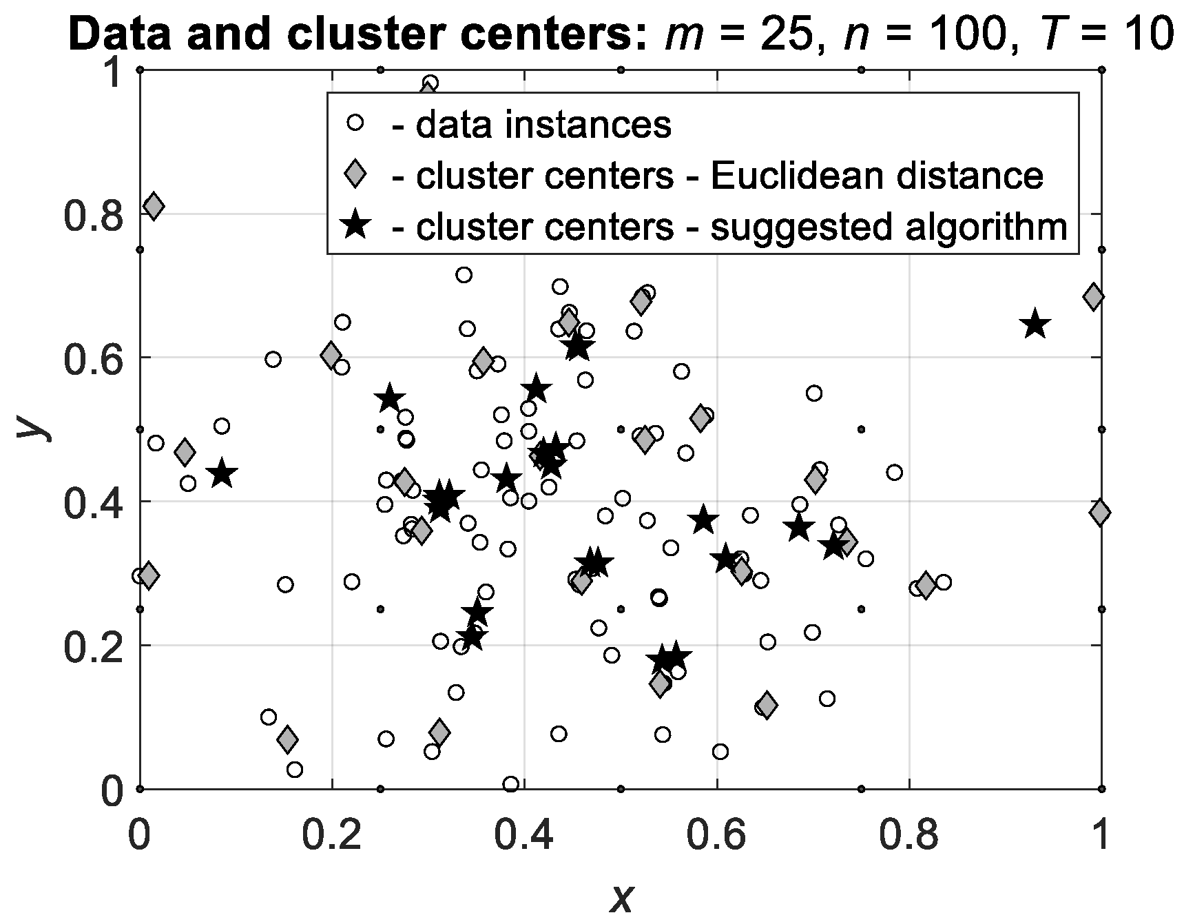
More clearly, the effect is observed on the data with several clusters. Figure 5 shows the results of Algorithms 1 and 2 applied to the data with $10$ predefined clusters.

It is seen that the cluster centers calculated by Algorithm 2 are concentrated at the real centers of the clusters and, as above, several centers are located at the same points. Hence, the suggested Algorithm 2 allows the more correct definition of the cluster centers and consequently, more correct clustering.

Now, let us apply Algorithms 1 and 2 to the well-known Iris dataset [29,30]. The dataset describes three types of Iris flowers using $150$ instances ($50$ for each type), and each instance includes four attributes—sepal length, sepal width, petal length, and petal width.

In the trials, we applied the algorithms to four pairs of attributes: sepal length and petal length, sepal length and petal width, sepal width and petal length, and sepal width and petal width. Results of Algorithms 1 and 2 are shown in Figure 6.

Similarly to the previous trials, the cluster centers found by the suggested Algorithm 2 are less dispersed than the cluster centers found by Algorithm 1. For large numbers of iterations (in the trials, we used $T=500$), the suggested Algorithm 2, in contrast to Algorithm 1, recognizes the cluster centers in hardly separable data, but does not always result in unambiguous cluster centers. In Figure 6b,c, where one cluster is separate and two are hardly separable, Algorithm 2 correctly defined three clusters, and in Figure 6a,d, where also one cluster is separate and two are non-separable, in two non-separable clusters, the algorithm defined four centers.

Finally, let us illustrate the dependence of the results of the suggested algorithm on the precision $\xi$ and, consequently, on the initial number $m$ of the clusters. The results of algorithms 1 and 2 with $\xi =0.1$, $m=100$ and $\xi =0.05$, $m=400$, are shown in Figure 7a and Figure 7b, respectively. Note that, in Figure 7a, the number of cluster centers is four times smaller than the number of instances, $m={\displaystyle \frac{1}{4}}n$, and in Figure 7b the number of cluster centers is equal to the number of instances, $m=n$.

It is seen that the cluster centers defined by Algorithm 2 with the precision $\xi =0.1$ and $\xi =0.05$ are concentrated in the same regions. The further increase in the precision provides the same results but requires a longer computation time.

To illustrate the usefulness of the suggested algorithm in recognition of the number of clusters and the analysis of the data structure, let us compare the results of the algorithm with the results obtained by the MATLAB^® fcm function [15] with three possible distance measures: Euclidean distance, Mahalanobis distance [16], and exponential distance [17]. These algorithms were applied to $n=200$ data instances distributed around $5$ centers; the obtained results are shown in Figure 8.

It is seen that the suggested algorithm (Figure 8a) correctly recognizes the real centers of the clusters and locates the cluster centers close to these real centers. In contrast, the known algorithms implemented in MATLAB^® do not recognize the real centers of the clusters, and consequently, do not define correct number of the clusters and locations of their centers. The function fcm with Euclidean and Mahalanobis distance measures (Figure 8b and Figure 8c) results in two cluster centers and the function fcm with exponential distance (Figure 8d) results in three cluster centers. Note that the use of the Euclidean and Mahalanobis distance measures leads to very similar results.

Thus, the recognition of real cluster centers can be conducted in two stages. At first, the cluster centers are defined by the application of the suggested algorithm to raw data, and secondly, the cluster centers are defined by the application of k-means to cluster centers found at the first stage. The resulting cluster centers indicate the real cluster centers.

4. Discussion

The suggested algorithm of fuzzy clustering follows the line of the c-means fuzzy clustering algorithms and differs from the known methods in the used distance measure.

The suggested fuzzy logical distance is based on the introduced semi-metric in the algebra of truth values with the uninorm and absorbing norm. The meaning of this semi-metric is the following.

Assume that some statements $A$ and $B$ are considered by a group of $d$ observers and each of the observers expresses an opinion about the truthfulness of these statements. Assuming that the observers are independent, then statements $A$ and $B$ can be considered as the points in the $d$-dimensional space, and then, the suggested semi-metric is a distance between these statements.

In other words, the fuzzy logical distance measures allow comparing the statements based on their subjective truthiness.

In this paper, we considered the fuzzy logical distance based on the uninorm and absorbing norm which, in their turn, use the sigmoid generating functions. As a result, the fuzzy logical distance effectively separates the data instances, which leads to the more precise calculation of the cluster centers and the faster convergence of the algorithm.

An additional advantage of the algorithm is the possibility of tuning its activity by two parameters: neutral element $\theta$ and absorbing element $\vartheta$. As indicated above, better clustering results can be obtained using non-equal values $\theta =0.475$ and $\vartheta =0.4$. An inequality of these parameters slightly disturbs the semi-metric properties of the distance measures; however, this leads to the better separation of close but different points.

The weakness of the algorithm is the need for the normalization of raw data and then the renormalization of the obtained cluster centers. However, since both operations are conducted in polynomial time, this disadvantage is not a serious drawback.

The suggested algorithm of fuzzy clustering can be used for solving the clustering problems instead of or together with the known algorithms, for the recognition of the centers of distributions of the data instances, and form a basis for the development of the methods of comparison of multivariate samples.

Despite the absence of theoretical limitations to the dimension of the data, the current implementation of the algorithm is aimed at two-dimensional data because of the visualization purposes. Further implementation will concentrate on avoiding this limitation and on the optimization of the code.

In addition, in the further research, we will consider the suggested algorithm in the framework of the possibilistic c-means clustering [31,32] and will address the relations between the suggested distance measure and the methods used in the possibilistic-fuzzy [33,34] and fuzzy-possibilistic [32,35] algorithms.

References

1. Raiffa, H. Decision Analysis. Introductory Lectures on Choices Under Uncertainty; Addison-Wesley: Reading, MA, USA, 1968. [Google Scholar]
2. Triantaphyllou, E. Multi-Criteria Decision Making Methods: A Comparative Study; Springer Science + Business Media: Dordrecht, The Netherlands, 2000. [Google Scholar]
3. López, L.M.; Ishizaka, A.; Qin, J.; Carrillo, P.A.A. Multi-Criteria Decision-Making Sorting. Methods Applications to Real-World Problems; Academic Press/Elsevier: London, UK, 2023. [Google Scholar]
4. Han, J.; Kamber, M.; Pei, J. Data Mining: Concepts and Techniques; Morgan Kaufmann/Elsevier: Waltham, MA, USA, 2012. [Google Scholar]
5. Ghanaiem, A.; Kagan, E.; Kumar, P.; Raviv, T.; Glynn, P.; Ben-Gal, I. Unsupervised classification under uncertainty: The distance-based algorithm. Mathematics 2023, 11, 4784. [Google Scholar] [CrossRef]
6. Ratner, N.; Kagan, E.; Kumar, P.; Ben-Gal, I. Unsupervised classification for uncertain varying responses: The Wisdom-In-the-Crowd (WICRO) algorithm. Knowl.-Based Syst. 2023, 272, 110551. [Google Scholar] [CrossRef]
7. Everitt, B.S.; Landau, S.; Leese, M.; Stahl, D. Cluster Analysis; Jonh Wiley & Sons: Chichester, UK, 2011. [Google Scholar]
8. Aggarwal, C.C. An introduction to cluster analysis. In Data Clustering: Algorithms and Applications; Aggarwal, C.C., Reddy, C.K., Eds.; Chapman & Hall/CRC/Taylor & Francis: London, UK, 2014. [Google Scholar]
9. Lloyd, S.P. Least squares quantization in PCM. IEEE Trans. Inf. Theory 1982, 28, 129–137. [Google Scholar] [CrossRef]
10. Forgy, E.W. Cluster analysis of multivariate data: Efficiency vs. interpretability of classifications. Biometrics 1965, 21, 768–769. [Google Scholar]
11. Hartigan, J.A.; Wong, M.A. A k-means clustering algorithm. J. R. Stat. Soc. Ser. C 1979, 28, 100–108. [Google Scholar]
12. MATLAB® Help Center. k-Means Clustering. Available online: https://www.mathworks.com/help/stats/k-means-clustering.html (accessed on 6 May 2025).
13. Bezdek, J.C. Fuzzy Mathematics in Pattern Classification. Ph.D. Thesis, Cornell University, Ithaca, NY, USA, 1973. [Google Scholar]
14. Bezdek, J.C. Pattern Recognition with Fuzzy Objective Function Algorithms; Springer: New York, NY, USA, 1981. [Google Scholar]
15. MATLAB® Help Center. Fuzzy Clustering. Available online: https://www.mathworks.com/help/fuzzy/fuzzy-clustering.html (accessed on 6 May 2025).
16. Gustafson, D.; Kessel, W. Fuzzy clustering with a fuzzy covariance matrix. In Proceedings of the IEEE Conference on Decision and Control, San Diego, CA, USA, 10–12 January 1979. [Google Scholar]
17. Gath, I.; Geva, A.B. Unsupervised optimal fuzzy clustering. IEEE Trans. Pattern Anal. Mach. Intell. 1989, 11, 773–780. [Google Scholar] [CrossRef]
18. Li, J.; Lewis, H.W. Fuzzy clustering algorithms—Review of the applications. In Proceedings of the IEEE International Conference on Smart Cloud, New York, NY, USA, 18–20 November 2016. [Google Scholar]
19. Höppner, F.; Klawonn, F.; Kruse, R.; Runkler, T. Fuzzy Cluster Analysis: Methods for Classification, Data Analysis and Image Recognition; Jonh Wiley & Sons: Chichester, UK, 2019. [Google Scholar]
20. Kagan, E.; Rybalov, A.; Siegelmann, H.; Yager, R. Probability-generated aggregators. Int. J. Intell. Syst. 2013, 28, 709–727. [Google Scholar] [CrossRef]
21. Kagan, E.; Rybalov, A.; Yager, R. Multi-Valued Logic for Decision-Making Under Uncertainty; Springer-Nature/Birkhäuser: Cham, Switzerland, 2025. [Google Scholar]
22. Yager, R.R.; Rybalov, A. Uninorm aggregation operators. Fuzzy Sets Syst. 1996, 80, 111–120. [Google Scholar] [CrossRef]
23. Rudas, I.J. New approach to information aggregation. Zb. Rad. 2000, 2, 163–176. [Google Scholar]
24. Fodor, J.; Yager, R.; Rybalov, A. Structure of uninorms. Int. J. Uncertain. Fuzziness Knowl.-Based Syst. 1997, 5, 411–427. [Google Scholar] [CrossRef]
25. Fodor, J.; Rudas, I.J.; Bede, B. Uninorms and absorbing norms with applications to image processing. In Proceedings of the 4th Serbian-Hungarian Joint Symposium on Intelligent Systems, Subotica, Serbia, 29–30 September 2006. [Google Scholar]
26. Rousseeuw, P.J. Silhouettes: A graphical aid to the interpretation and validation of cluster analysis. J. Comput. Appl. Math. 1987, 20, 53–65. [Google Scholar] [CrossRef]
27. Dunn, J.C. A fuzzy relative of the ISODATA process and its use in detecting compact well-separated clusters. J. Cybern. 1973, 3, 32–57. [Google Scholar] [CrossRef]
28. Dunn, J.C. Well-separated clusters and optimal fuzzy partitions. J. Cybern. 1974, 4, 95–104. [Google Scholar] [CrossRef]
29. Fisher, R.A. The use of multiple measurements in taxonomic problems. Ann. Eugen. 1936, 7, 179–188. [Google Scholar] [CrossRef]
30. Iris Dataset. UC Irvine Machine Learning Depository. Available online: https://archive.ics.uci.edu/dataset/53/iris (accessed on 6 May 2025).
31. Krishnapuram, R.; Keller, J. The possibilistic c-means algorithm: Insights and recommendations. IEEE Trans. Fuzzy Syst. 1996, 4, 385–393. [Google Scholar] [CrossRef]
32. Pal, N.R.; Pal, K.; Bezdek, J.C. A mixed c-means clustering model. In Proceedings of the IEEE International Conference on Fuzzy Systems, Barcelona, Spain, 1–5 July 1997. [Google Scholar]
33. Pal, N.K.; Pal, K.; Keller, K.M.; Bezdek, J.C. A possibilistic fuzzy c-means clustering algorithm. IEEE Trans. Fuzzy Syst. 2005, 13, 517–530. [Google Scholar] [CrossRef]
34. Chen, Y.; Zhou, S. Revisiting possibilistic fuzzy c-means clustering using the majorization-minimization method. Entropy 2024, 26, 670. [Google Scholar] [CrossRef] [PubMed]
35. Naghi, M.-B.; Kovacs, L.; Szilagyi, L. A generalized fuzzy-possibilistic c-means clustering algorithm. Acta Univ. Sapientiae Inform. 2023, 15, 404–431. [Google Scholar] [CrossRef]
Figure 1. (a) Fuzzy logic distance d i s t θ , ϑ x , y between the values x , y 0 , 1 with θ = ϑ = 0.5 ; and (b) Euclidean distance between the values x , y 0 , 1 .
Mathematics 13 01661 g001
Figure 2. Example of the data and the resulting cluster centers for a single cluster of normally distributed instances. The number of instances is n = 100 , the number of clusters is m = 25 , and the number of iterations T = 10 . Initially, the cluster centers are in the nodes of the grid and are depicted by black points. The instances are distributed normally around the mean μ = 0.5 and are shown by white circles. The cluster centers calculated by Algorithm 1 with the Euclidean distance are depicted by gray diamonds and the cluster centers calculated by the Algorithm 2 with fuzzy logical distance are depicted by black pentagrams.
Mathematics 13 01661 g002
Figure 3. The average Dann coefficient with respect to the initial number of clusters. The real number of clusters is m = 10 and the algorithms started with a single cluster and continued up to 100 clusters.
Mathematics 13 01661 g003
Figure 4. Data with two predefined clusters and cluster centers calculated by the Algorithms 1 and 2: (a) number of clusters m = 25 ; and (b) number of clusters m = 9 .
Mathematics 13 01661 g004
Figure 5. Data with ten predefined clusters and cluster centers calculated by algorithms 1 and 2: (a) number of clusters m = 25 ; and (b) number of clusters m = 9 .
Mathematics 13 01661 g005
Figure 6. Iris dataset and cluster centers calculated by the algorithms 1 and 2: (a) sepal length and petal length, (b) sepal width and petal width, (c) sepal length and petal width, and (d) sepal width and petal length. In the figures, the number of clusters m = 25 , the number of instances n = 150 and the number of iterations at each step is T = 500 .
Mathematics 13 01661 g006
Figure 7. Data with ten predefined clusters and cluster centers calculated by the Algorithms 1 and 2: (a) precision ξ = 0.1 and number of clusters m = 100 ; and (b) precision ξ = 0.05 and number of clusters m = 400 .
Mathematics 13 01661 g007
Figure 8. Cluster centers calculated by the suggested Algorithm 2 (a) and by the MATLAB® fcm function with the Euclidean (b), Mahalanobis (c), and exponential (d) distance measures. In all cases, the real number of clusters is 5 and the number of data instances is n = 200 . Algorithm 2 starts with m = 25 clusters and is terminated after 10 iterations, and function fcm defines an optimal number of clusters by trials with a number of clusters from 2 to 11 .
Mathematics 13 01661 g008