Abstract
In response to the threat assessment challenge posed by unmanned aerial vehicles (UAVs) in air defense operations, this paper proposes a dynamic assessment model grounded in fuzzy multi-attribute decision making. First, a three-dimensional evaluation index system is established, encompassing capability, opportunity, and intention. Quantification functions for assessing the threat level of each attribute are then designed. To account for the temporal dynamics of the battlefield, an innovative fusion approach is developed, integrating inverse Poisson distribution time weights with subjective–objective comprehensive weighting, thereby establishing a dynamic variable weight fusion mechanism. Among these, the subjective weights are determined by integrating the intention probability matrix, effectively incorporating the intentions into the threat assessment process to reflect their dynamic changes and enhancing the overall evaluation accuracy. Leveraging the improved technique for order preference by similarity to ideal solution (TOPSIS), the model achieves threat prioritization. Experimental results demonstrate that this method significantly enhances the reliability of threat assessments in uncertain and dynamic battlefield environments, offering valuable support for air defense command and control systems.
MSC:
90B50; 90C70
1. Introduction
In recent years, unmanned combat and intelligent warfare have emerged as key research areas. Since the onset of the Russia–Ukraine conflict in 2022, unmanned aerial vehicles (UAVs) have become an indispensable component on the battlefield. Ukraine successfully employed TB-2 UAVs to conduct precise strikes against Russian armored formations and logistics hubs, achieving the paralysis of high-value targets at minimal cost. The application scope of UAVs has evolved from tactical reconnaissance to strategic strikes, significantly expanding the threat dimension. During combat operations, targets with higher threat levels are typically categorized as high-value targets, necessitating the allocation of additional resources for preemptive attacks or interference. Against this backdrop, a systematic assessment of UAV threats can quantify target importance by integrating multi-source intelligence data, thereby enabling commanders to construct dynamic threat situation maps. This supports the efficient coordination of air defense units, the optimal allocation of interception resources, and the intelligent formulation of defense strategies.
The existing threat assessment methods primarily encompass evidence theory [1], fuzzy reasoning [2,3], Bayesian networks [4], multi-attribute decision making theory [5,6], cloud model theory [7], and neural networks [8]. While the specific research targets of these methods may differ, their underlying principles demonstrate broad applicability. When applied to the threat assessment of UAVs, each method demonstrates distinct characteristics due to its inherent theoretical foundations, as detailed in Table 1.

Table 1.
The comparison among target threat assessment methods.
In actual combat, assessing the threat level of targets involves integrating various factors. While algorithms excel at rapidly processing data, the experience and judgment of commanders remain invaluable and irreplaceable. To address the “human-in-the-loop” requirement in military decision making, it is essential to combine algorithms with the knowledge and expertise of military professionals. In a battlefield environment characterized by multi-attribute considerations, high dynamics, and intense adversarial interactions, multi-attribute decision making theory stands out compared to other threat assessment methods. It demonstrates core advantages such as exceptional battlefield adaptability, effective human–machine collaboration, and flexible scalability. This approach addresses key deficiencies in other methods for assessing the threats posed by UAVs on the battlefield, making it a prominent focus in threat assessment research. Over the past 20 years, multi-attribute decision making methods have accounted for 44% of solutions to target threat assessment problems [9].
Furthermore, given the uncertainty and dynamic nature of battlefield situation information, the advancement of fuzzy theory, particularly the intuitionistic fuzzy set [10], has introduced revolutionary changes to military threat assessment. It not only handles uncertain information effectively but also integrates the subjective judgments of experts, thereby compensating for the limitations of traditional multi-attribute decision making methods in dynamic and uncertain environments [11]. This enhances the alignment of the threat assessment model with the requirements of real combat scenarios. Consequently, the fuzzy multi-attribute decision analysis method, which incorporates fuzzy theory and demonstrates an excellent capacity for representing uncertainty and directly calculating threat levels, has garnered significant attention from researchers within the context of fuzzy decision making [11,12,13,14,15,16,17,18]. When applied to threat assessment, multi-attribute decision making methods primarily encompass four key aspects: the selection of threat assessment attributes, the description and quantification of these attributes, the determination of attribute weights, and the choice of target threat ranking methods. Nevertheless, the above methods still fall short of fully addressing the needs of UAV threat assessment in practical scenarios, as specifically reflected in the following aspects:
- In the selection of threat assessment attributes, most research primarily emphasizes the direct threat posed by the target to our units during threat assessment and seldom considers the influence of external environmental factors [2,5,11,12,14,15,16,17,18,19,20]. Direct threat attributes typically include the target’s static combat capabilities and dynamic situational information [12]. The threat from UAVs is first determined by their inherent capabilities and then manifested through specific events driven by intention. The target operational intention indicator focuses on possible actions the target may take, which evolve based on battlefield command decisions, affecting the threat level. Evaluating these intentions helps anticipate the opponent’s combat strategies, allowing for proactive preparation. Although significant research progress has been made in UAV intention recognition, current target threat assessment methods still lack effective integration of combat intentions.
- Many existing methods for describing and quantifying threat assessment attributes simplify the process by relying on precise real-number data inputs [5,11,12,14,15,16,17,18,19,20]. However, in real combat, information from various sources is often heterogeneous, with varying accuracy levels across sensors. Some methods [19,20] fail to account for the inherent uncertainty in this information, undermining the scientific validity of the results. Given the complexity of the combat environment, both sensor-derived data and human-based judgments exhibit degrees of fuzziness and uncertainty. When employing fuzzy multi-attribute decision making for threat assessment, effectively quantifying, transforming, and standardizing the raw data of threat assessment attributes becomes critical for subsequent threat prioritization.
- In the determination of attribute weights, traditional multi-attribute decision making threat assessment methods are static, treating each time point as an independent event and failing to account for the timing of the target or dynamic changes on the battlefield [2,11,12,14,19,20]. However, target threat assessment is inherently dynamic and requires integrating information from multiple time points for a comprehensive evaluation. Therefore, it is crucial to aggregate multi-time attribute data into a unified matrix across the assessment period, enabling reliable threat assessment in dynamic environments. Additionally, some studies [6] rely on linear weighted combinations for fixed composite weights, leading to a lack of differentiation when addressing multiple targets, which necessitates improvement.
- In multi-attribute decision making, selecting the target threat ranking method constitutes the final step. Nevertheless, the traditional TOPSIS method, which depends on Euclidean distance, struggles to effectively process non-membership and hesitation degree information inherent in the intuitionistic fuzzy environment. Therefore, it is necessary to enhance the TOPSIS method to improve its applicability in fuzzy decision-making contexts.
How to reasonably incorporate the target’s combat intention information into UAV threat assessment, how to appropriately characterize the heterogeneity of attributes and quantify the uncertainty of raw data, how to scientifically determine the weights of assessment attributes to emphasize the dynamic nature of threat assessment, and how to select a ranking method suitable for the fuzzy decision-making context are all critical factors in achieving more accurate threat assessment results. To tackle these challenges, this paper proposes a multi-time dynamic threat assessment model for UAVs based on fuzzy multi-attribute decision making with integrated intentions. The primary contributions are as follows:
- This article constructs a UAV threat assessment index system by considering three critical aspects: target capability, target intention, and target opportunity, integrating both the intention and environmental condition attributes into the framework. Furthermore, threat membership functions for each attribute are systematically designed based on the practical requirements of UAV combat scenarios.
- By integrating fuzzy theory with multi-attribute decision making theory, the fuzziness inherent in sensor data errors or subjective judgments is preserved. Specifically, this integration manifests in two key aspects. First, specific threat attributes are fuzzified to address the challenge of “quantifying individual attributes using fuzzy mathematics.” This involves mapping raw data into representation forms within the fuzzy mathematics framework, such as fuzzy linguistic terms, interval numbers, or triangular fuzzy numbers. Second, data formats are standardized to resolve the issue of “enabling all attributes to be collaboratively analyzed under a unified mathematical framework.” All intermediate fuzzy mathematical representations of heterogeneous evaluation attributes are systematically converted into intuitionistic fuzzy numbers, ensuring consistent input for subsequent threat assessment ranking.
- The inverse Poisson distribution is utilized to calculate the time-sequence weights based on real-time situational awareness, enabling effective integration of evaluation information across multiple time points. Objective weights are formulated using cosine intuitionistic fuzzy entropy to capture the dynamic nature of threat assessment. Additionally, a subjective weight determination method incorporating the intention probability matrix is developed to effectively consolidate target combat intention information. Simultaneously, a comprehensive variable weight fusion approach considering IFS scores is proposed to differentiate the integrated weights among multiple targets.
- The TOPSIS method based on the hesitation-degree-weighted similarity measure, which is particularly suited for intuitionistic fuzzy environments, is employed for threat ranking. This method comprehensively accounts for the interactions among membership degree, non-membership degree, and hesitation degree, thereby enhancing the robustness of decision making through a weighted scoring mechanism.
After simulation experiments and analysis, the threat assessment model we proposed is capable of accurately evaluating the threat level of UAVs and demonstrates superior effectiveness compared to the models presented in [12,18]. The remainder of this paper is structured as follows: Section 2 reviews the related work on fuzzy multi-attribute decision making. Section 3 elaborates on the proposed model in detail. Section 4 carries out simulation experiments in a predefined scenario to validate the model’s effectiveness and conducts comparative experimental analysis with the other two models. Section 5 concludes the paper with a summary.
2. Related Works
2.1. Intuitionistic Fuzzy Sets
Fuzzy theory was initially introduced by Zadeh in 1965 [21] to address uncertainties that traditional set theory is incapable of capturing. In 1986, Atanassov extended fuzzy set theory [10] by proposing the concept of intuitionistic fuzzy sets, which not only evaluates the membership degree of elements but also integrates non-membership degrees and hesitation margins. This enhanced framework endows the theory with a unique capability to tackle complex military decision-making problems effectively.
Definition 1
([10]). Given a universe of discourse , an intuitionistic fuzzy set (IFS) defined on X can be expressed in the following form:
where denote the membership degree and non-membership degree of , respectively, and for all on , there is the following:
The hesitation degree for all is defined as follows:
For ease of representation, an intuitionistic fuzzy number (IFN) is defined as , where , , and is satisfied.
Definition 2
([22]). Assuming any , , is a positive real number, the operational rules for IFN are defined as follows:
Definition 3
([23]). Let , be an IFN and be a weighting vector that satisfies , , . The intuitionistic fuzzy weighted averaging (IFWA) operator is defined as a mapping :
2.2. Intuitionistic Fuzzy Multi-Attribute Decision Making
Multi-attribute decision making (MADM) theory is a widely adopted approach for addressing threat assessment problems. In 2000, Qu et al. [6] introduced a threat assessment model and method grounded in MADM. In 2016, Fu et al. [19] developed an index system for evaluating the threat levels of targets in air defense systems, integrating both qualitative and quantitative aspects. However, these studies did not adequately account for the uncertainty and dynamics inherent in battlefield situation information. Consequently, under the framework of fuzzy decision making, significant attention has been directed toward the intuitionistic fuzzy multi-attribute decision making (IFMADM) method. In 2019, Xiao et al. [11] proposed an air target threat assessment method based on the intuitionistic fuzzy analytic hierarchy process (IF-AHP), utilizing intuitionistic fuzzy numbers to characterize the interrelationships among evaluation indicators. In 2022, Qi et al. [12] constructed an intuitionistic fuzzy technique for order preference by similarity to ideal solution (TOPSIS) model and a variable weight VIKOR model to comprehensively assess the threats associated with both static and dynamic attributes of targets. IFMADM represents an extension of traditional MADM within the context of fuzzy information, further incorporating the non-membership function to enable a more precise representation of uncertain situational information.
In recent years, numerous MADM methods based on intuitionistic fuzzy sets have been developed. In 2008, Xu et al. investigated dynamic MADM problems with intuitionistic fuzzy information, defining intuitionistic fuzzy variables and proposing two aggregation operators [13]. In 2014, Huang et al. [14] integrated intuitionistic fuzzy sets and fuzzy integrals into the threat assessment domain, presenting a threat estimation method based on the Choquet integral of intuitionistic fuzzy sets. Wang et al. [2] introduced an intuitionistic fuzzy similarity measurement reasoning model for ranking air attack target threats. In 2015, Ehsan et al. [15] applied fuzzy set theory to precisely describe the threat process, introducing 11 parameters for the first time in threat assessment and constructing a threat assessment model for air defense environments. However, these studies exhibit static characteristics and face challenges in integrating with dynamic combat situations. To address this, Zhang et al. [16] proposed a multi-target threat assessment method for air combat by combining intuitionistic fuzzy entropy with a dynamic intuitionistic fuzzy approach, utilizing the Poisson distribution to process multi-temporal situation information and calculate time series weights. In 2018, Zhang et al. [5] established a multi-target threat assessment and ranking model for air targets based on intuitionistic fuzzy entropy and dynamic VIKOR. In 2019, Feng et al. [17] developed an improved generalized intuitionistic fuzzy soft set (GIFSS) method, employing the inverse Poisson distribution to determine time series weights and weigh different times of GIFSS for dynamic air target threat assessment. In 2020, under the framework of IFMADM, Gao et al. [18] proposed a target threat assessment method based on three-party decision making, deriving time series weights using the inverse form of the Poisson distribution.
Fundamentally, IFMADM involves selecting a specific alternative from multiple options based on various criteria. In the past, several solution methods for IFMADM have been developed, including aggregation operator-based methods [24], TOPSIS [25], VIKOR [26], and others. Among these, TOPSIS inherently supports the integration of extended methods, such as fuzzy sets and intuitionistic fuzzy sets, to enhance the characterization of uncertain threat information, making it a particularly suitable tool for addressing IFMADM problems.
TOPSIS, introduced by Hwang and Yoon [27], is a method for ranking alternatives based on their proximity to the ideal solution. The core principle of the TOPSIS evaluation method involves identifying the positive and negative ideal solutions among the finite options based on the normalized decision matrix. By comprehensively analyzing the distances between each evaluated alternative and both the positive and negative ideal solutions, the relative closeness coefficient of each alternative to the ideal solution is determined. This coefficient serves as the basis for evaluating the superiority or inferiority of the alternatives and enables their ranking. In TOPSIS, weight determination plays a critical role. For the same threat assessment model, assigning different weights to one or several attributes may lead to entirely distinct assessment results, directly impacting the correctness and rationality of the threat judgment. Some scholars categorize the methods for calculating attribute weights into three types, as shown in Table 2. Since using any single category of method has inherent limitations, most existing studies adopt a hybrid weight that integrates subjective and objective weights. For instance, Li et al. [20] used AHP and the entropy weight method to assign weights separately and introduced a distance function to calculate the combined weight coefficient, ensuring that the assessment results reflect both expert subjective judgment and data objectivity. Various methods exist for determining the distribution coefficients of subjective and objective weights, such as game theory optimization, the least squares principle, variance maximization, deviation maximization, and relative information entropy. Currently, no unified standard exists, and decision-makers can select appropriate methods based on different mathematical principles.
Table 2.
Three categories for calculating attribute weights.
3. The Proposed Dynamic Threat Assessment Model
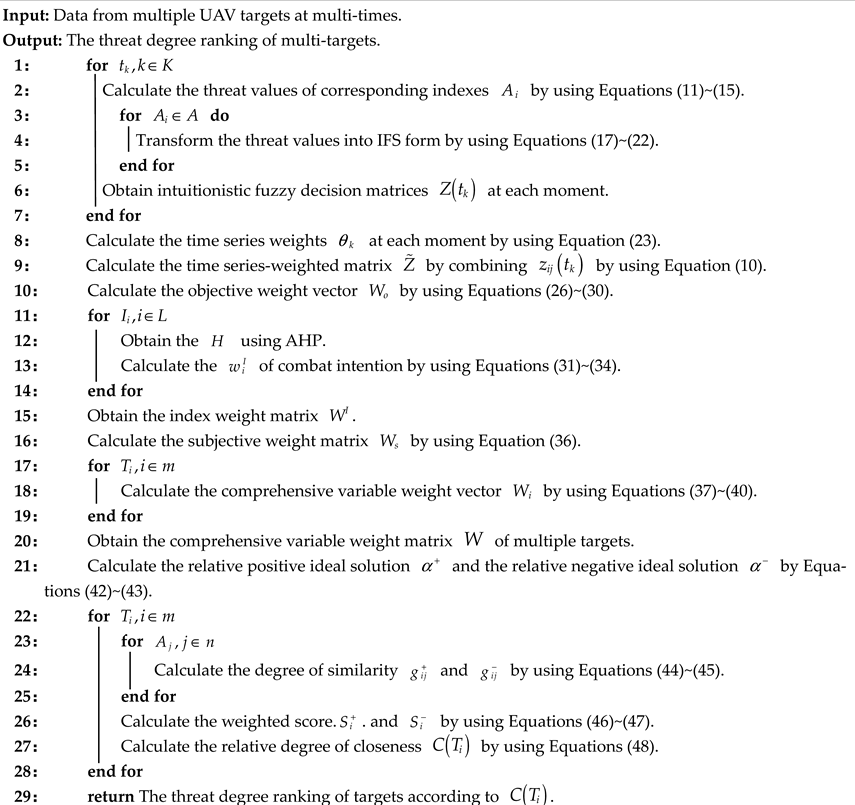
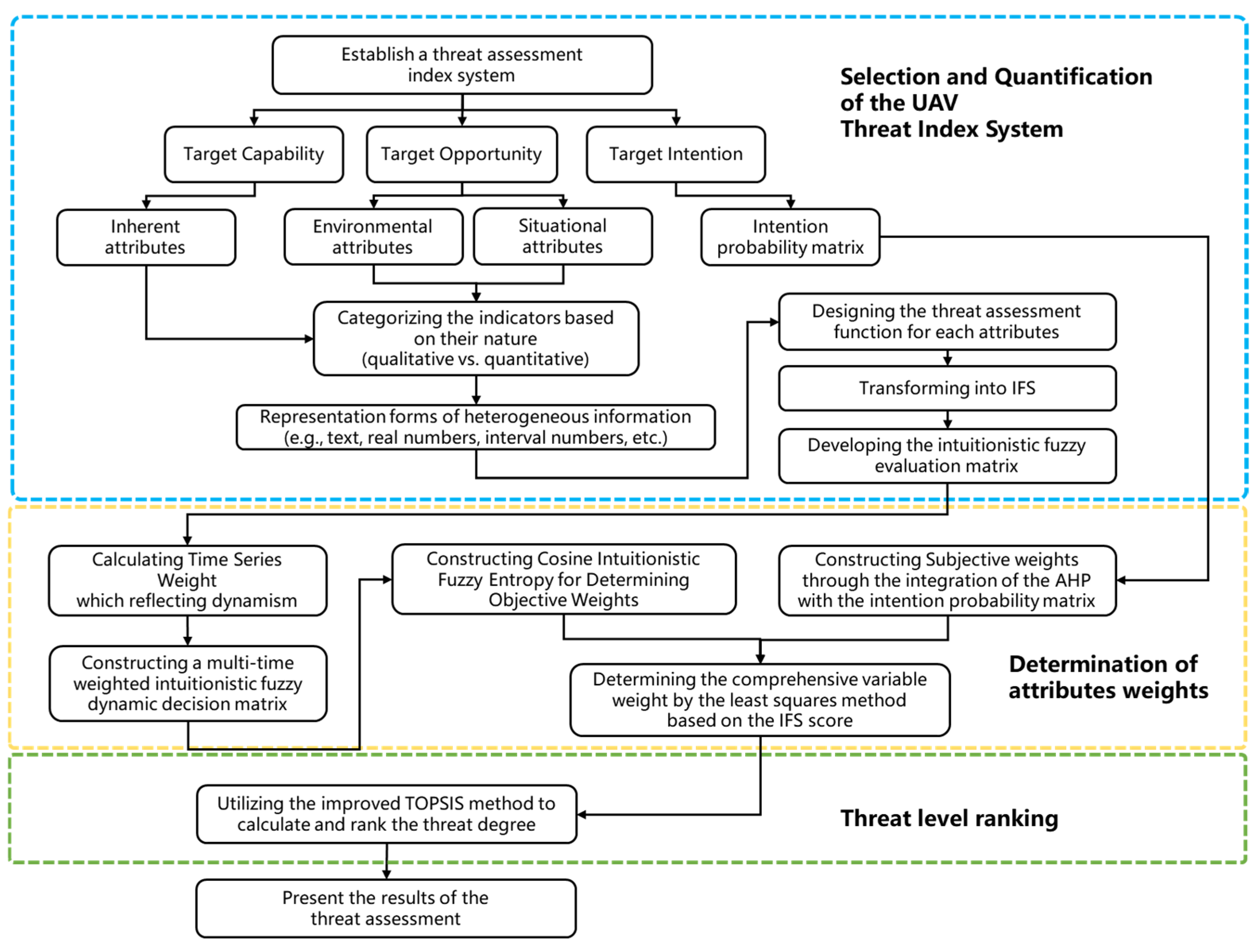
This section presents a detailed description of the proposed threat assessment model based on fuzzy multi-attribute decision making, specifically designed for UAV combat scenarios. The assessment process of the proposed model is illustrated in Figure 1. The entire threat assessment process is implemented using Algorithm 1, with its pseudocode provided in Algorithm 1. The mathematical formulations relevant to the proposed model are described as follows:
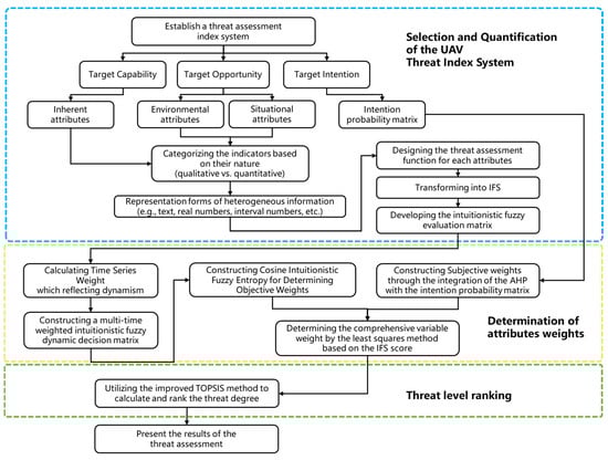
Figure 1.
The proposed dynamic threat assessment model for UAVs.
Suppose the defended assets are A, and the set of enemy UAV targets consists of m targets, with n threat assessment attributes for each UAV. Additionally, represents the set of K evaluation time points, represents the L intention of UAV, and denotes the temporal weights associated with K time points. At time point , , the subjective weight matrix for the UAV target is denoted as , the objective weight vector is represented as , and the comprehensive variable-weighted matrix is defined as . Let the decision evaluation matrix be denoted as , where represents the evaluation value of the attribute of target at time . In this paper, the value of is expressed using an intuitionistic fuzzy number, denoted as .
| Algorithm 1: The dynamic threat assessment algorithm |
 |
3.1. UAV Threat Assessment Index System
3.1.1. Selection of UAV Threat Assessment Indexes
In the context of single-point area air defense, the assets protected by air defense units are clearly defined and fixed. Therefore, in such air defense scenarios, there is no need to consider the importance of the defended assets. Instead, it is sufficient to evaluate the threat levels of air attack targets based on the parameters provided by the air defense reconnaissance system. The general framework for threat assessment involves extracting and quantifying the threat attributes associated with a target and then deriving relevant threat values. Selecting appropriate threat attributes constitutes the first critical step in this process. During target threat assessment, evaluation attributes directly influence the assessment results. Generally, a greater number of attributes implies richer information coverage and more accurate results. However, an excessive number of indicators may lead to redundant information, increased computational complexity, and potential conflicts between indicators. Given the real-time requirements of air defense systems, the selection of target threat attributes should be carefully controlled to avoid unnecessary complexity. Based on an extensive literature review, this paper concludes that the threat posed by UAVs in combat environments should be assessed from three key aspects: target capability, target intention, and target opportunity.
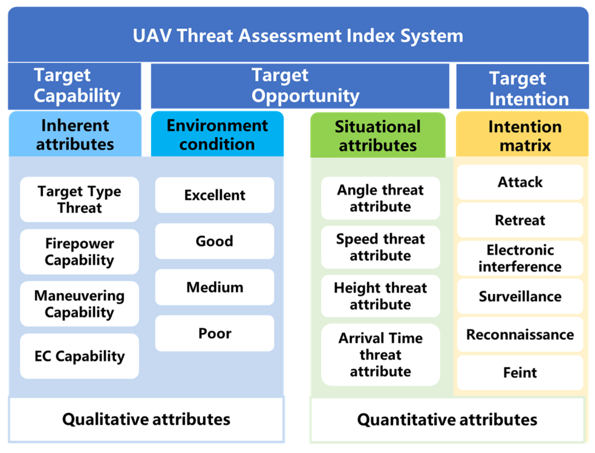
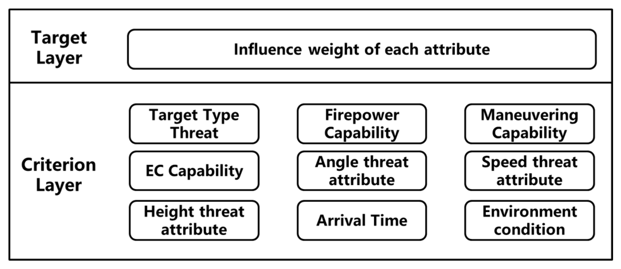
In threat assessment, the inherent attributes determine the capabilities of UAVs. UAV types can be categorized into attack UAVs, jamming UAVs, reconnaissance UAVs, and decoy UAVs. Different types of targets pose varying levels of threat to the defended assets. This paper selects target type threat, firepower strike capability, maneuvering capability, and electronic countermeasure (EC) capability as attributes for qualitatively analyzing the target capability. The actual situational attributes of UAVs determine their potential impact during missions, which reflects the target opportunity. Moreover, the battlefield environment is a critical factor influencing UAV combat effectiveness. Better environmental conditions are more conducive to maximizing UAV performance; therefore, this paper integrates environmental conditions into the target opportunity assessment. The target’s intention focuses on the possible actions that the threat source may take. Similarly, the output of UAV intention recognition at the current moment is used as input for the threat assessment index system. The final constructed UAV threat assessment index system is illustrated in Figure 2.
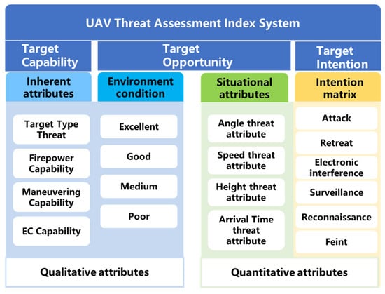
Figure 2.
UAV threat assessment index system.
3.1.2. Quantification of UAV Threat Assessment Indexes
After determining the corresponding threat assessment attributes, it is essential to quantify these attributes to derive the relevant threat values. The motion information associated with the target situation threat reflects the target opportunity and serves as a quantitative indicator that can be precisely acquired through various sensors. In such cases, membership functions are employed to process these indicators. Conversely, target capability and environmental conditions are qualitative indicators. These indicators cannot be directly measured by sensors in a specific numerical form and must instead be assessed by combat personnel based on their expertise. In this paper, human experience information is qualitatively characterized using fuzzy language and triangular fuzzy numbers.
Target Capability
The quantification of target ability attributes is achieved through the application of fuzzy evaluation language. The detailed procedure is outlined below.
- Step 1: Define an appropriate language assessment scale. If the linguistic scale for target capability is divided into L levels, then the fuzzy evaluation linguistic scale set can be expressed as . In this paper, the value of L is determined as 11, corresponding to the following levels: maximal, very large, large, relatively large, slightly large, moderate, slightly small, relatively small, small, very small, and minimal.
- Step 2: Based on the degree of certainty in the decision-makers’ judgment of the results, a result certainty degree vector is constructed. In this study, C is categorized into 5 levels, specifically absolutely certain, fairly certain, moderately certain, slightly certain, and uncertain.
- Step 3: Based on the decision-maker’s judgment, the fuzzy evaluation language reflecting the degree of certainty in the decision-maker’s own judgment is obtained.
Target Opportunity
- 1.
- Angle threat attribute
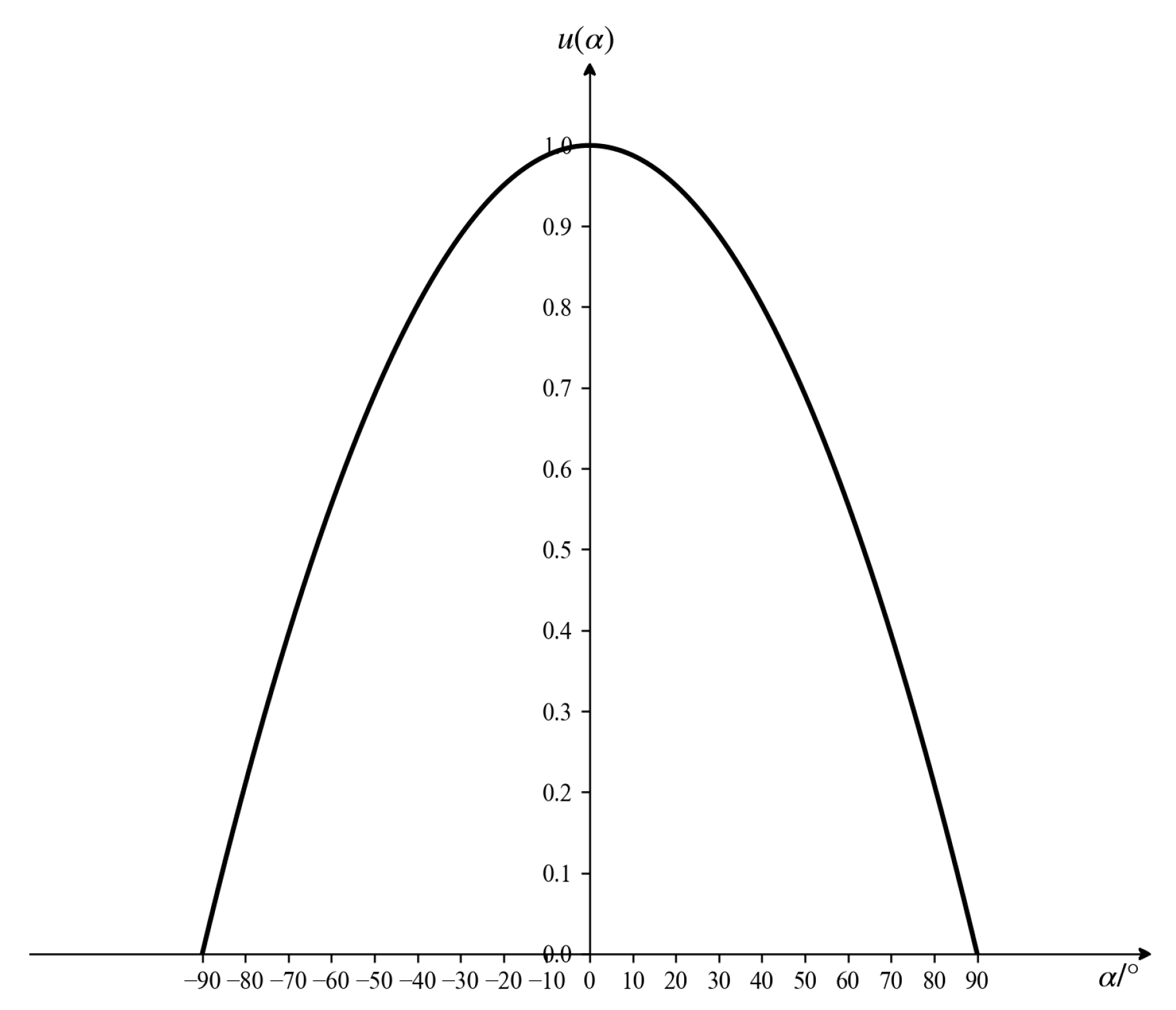
The target’s entry angle reflects its flight direction relative to the defended asset, specifically the angle between the target’s trajectory and the extended line connecting the target to the defended asset. When the target attacks the defended asset, its flight direction must point toward the asset side. A larger entry angle indicates a more evident attack intention; as this angle decreases, the threat level gradually diminishes. When the angle equals 0, it signifies that the target is moving away from the defended asset, at which point the threat value becomes zero. The membership function for the entry-angle-based threat assessment is established as shown in Figure 3, with the corresponding mathematical expression provided below:
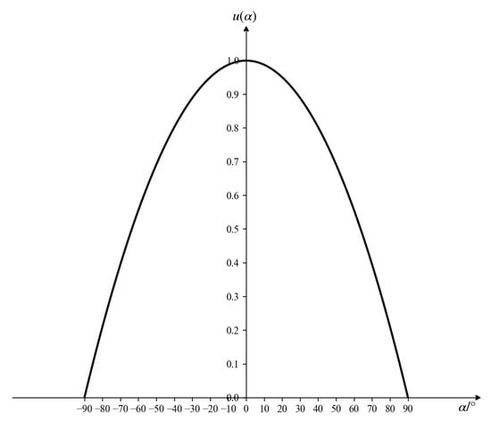
Figure 3.
Angle threat function.
- 2.
- Speed threat attribute
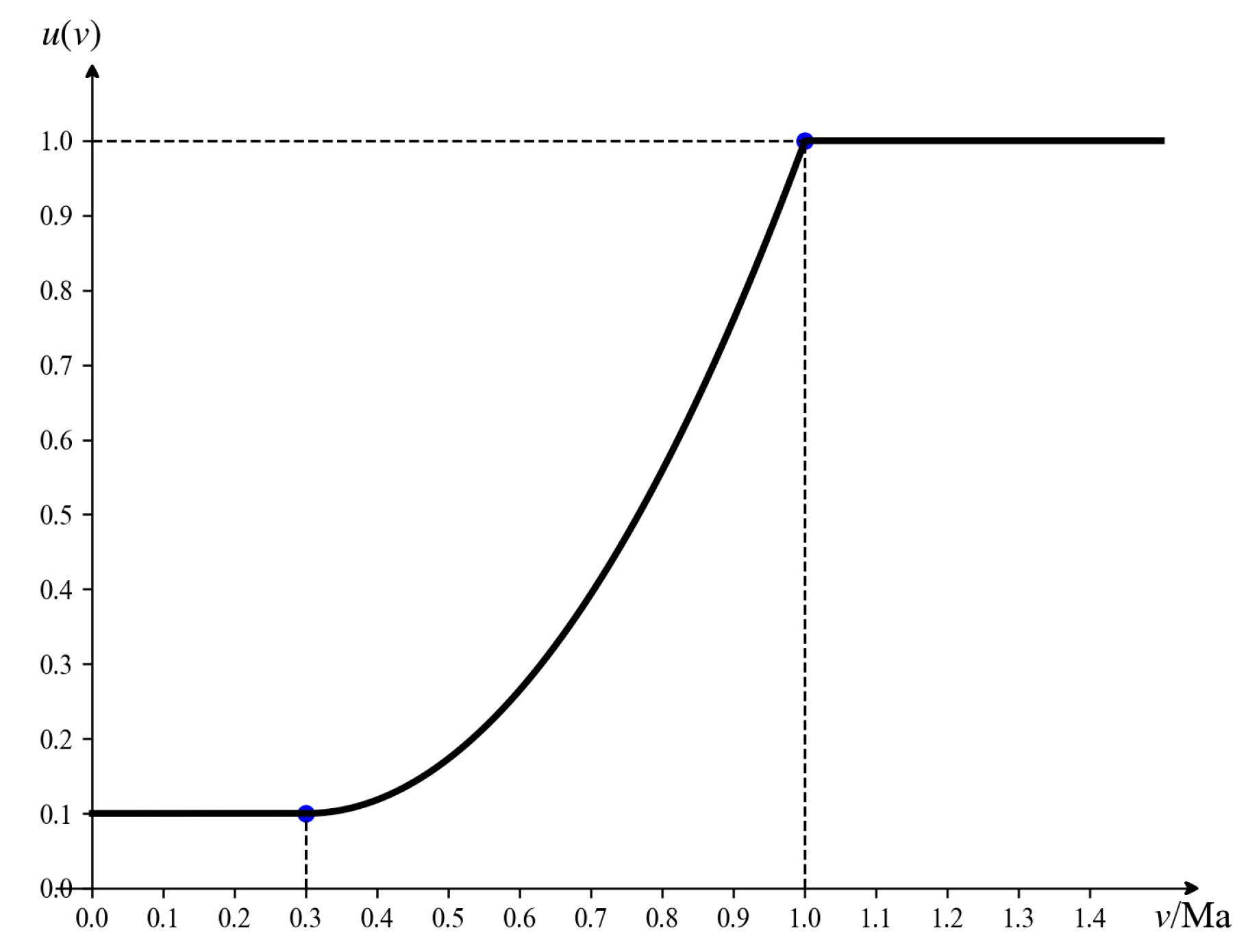
In general, the faster an incoming target flies, the more challenging it becomes to intercept, and the greater the threat posed to the defense position. Focusing solely on target speed, fixed-wing UAVs typically fly faster than rotary-wing UAVs. Currently, operational fixed-wing UAVs can reach speeds of approximately 1 Mach. If a UAV’s speed exceeds 1 Mach, its penetration and high-speed maneuverability are significantly enhanced, posing a substantial threat with a quantified threat value of 1. Conversely, if the UAV’s speed is below 0.3 Mach, it becomes easier for the defense system to detect and intercept it, allowing traditional air defense systems to handle it effectively, resulting in a lower threat level with a quantified threat value of 0.1. Given the fluctuations in the target’s flight state, representing the UAV’s speed using interval numbers improves the robustness and fault tolerance of threat assessment. A rising piecewise function is employed to construct the membership function for speed-related threats, as illustrated in Figure 4. When the input interval is provided, the corresponding mathematical expression of is as follows:
where , and .
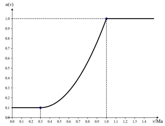
Figure 4.
Speed threat function.
- 3.
- Height threat attribute
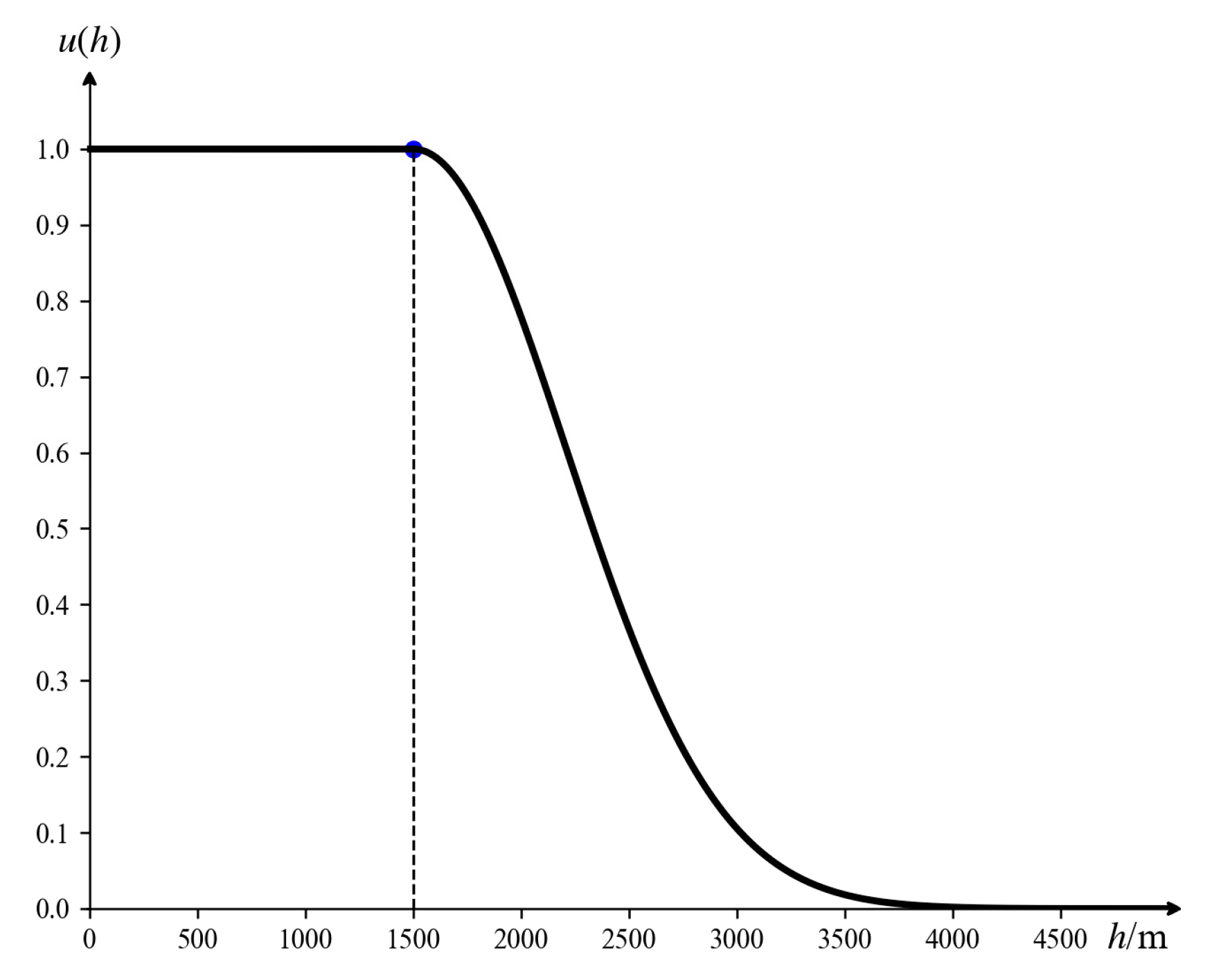
The lower the height of the incoming target, the easier it is to avoid radar detection and the more direct the attack on the defense asset becomes. Consequently, as the target height decreases, its threat level progressively increases. Given potential errors in data collection, interval numbers are employed to represent the uncertainty in height. The membership function for the threat associated with target height is established, as shown in Figure 5. When the input interval is provided, the corresponding mathematical expression of is as follows:
In this article, , , and the unit of h is meters (m).

Figure 5.
Height threat function.
- 4.
- Arrival Time threat attribute
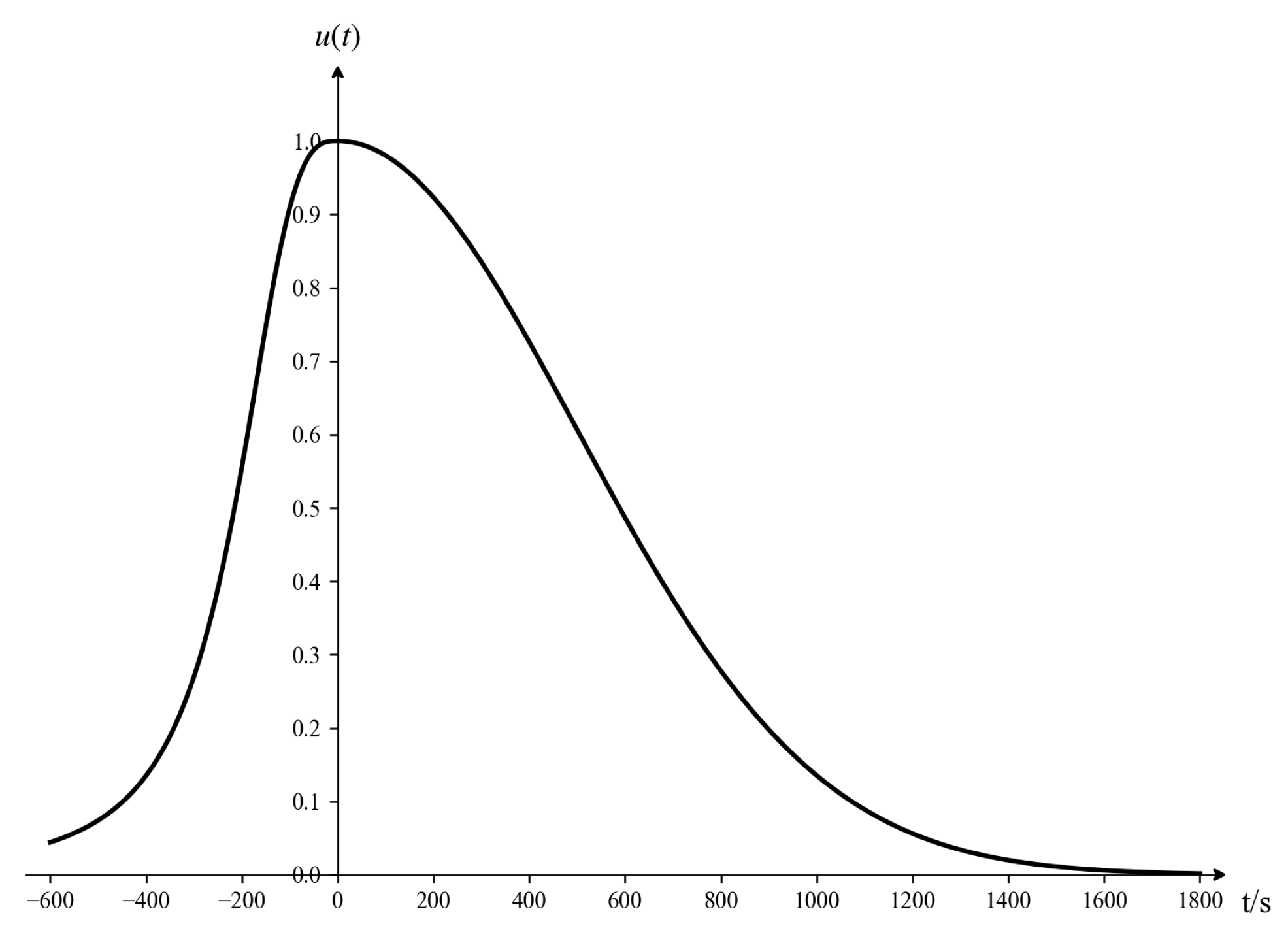
The arrival time is defined as the duration required for a target to reach the near-boundary of the air defense position. Owing to various uncertain factors, the arrival time obtained by sensors is not an exact real number but rather an interval. The calculation of arrival time must account for both the time when the target approaches the defended asset and the negative value representing the time when the target moves away. This consideration arises because the threat posed by the target is not limited to the approach phase; the departure phase may also influence the overall situation. Based on this understanding, the membership function for the threat associated with arrival time is established, as depicted in Figure 6. When the input interval is provided, the corresponding mathematical expression of is as follows:
In this article, = , = , a = 0, and the unit of t is seconds (s).

Figure 6.
Arrival time threat function.
- 5.
- Environment index
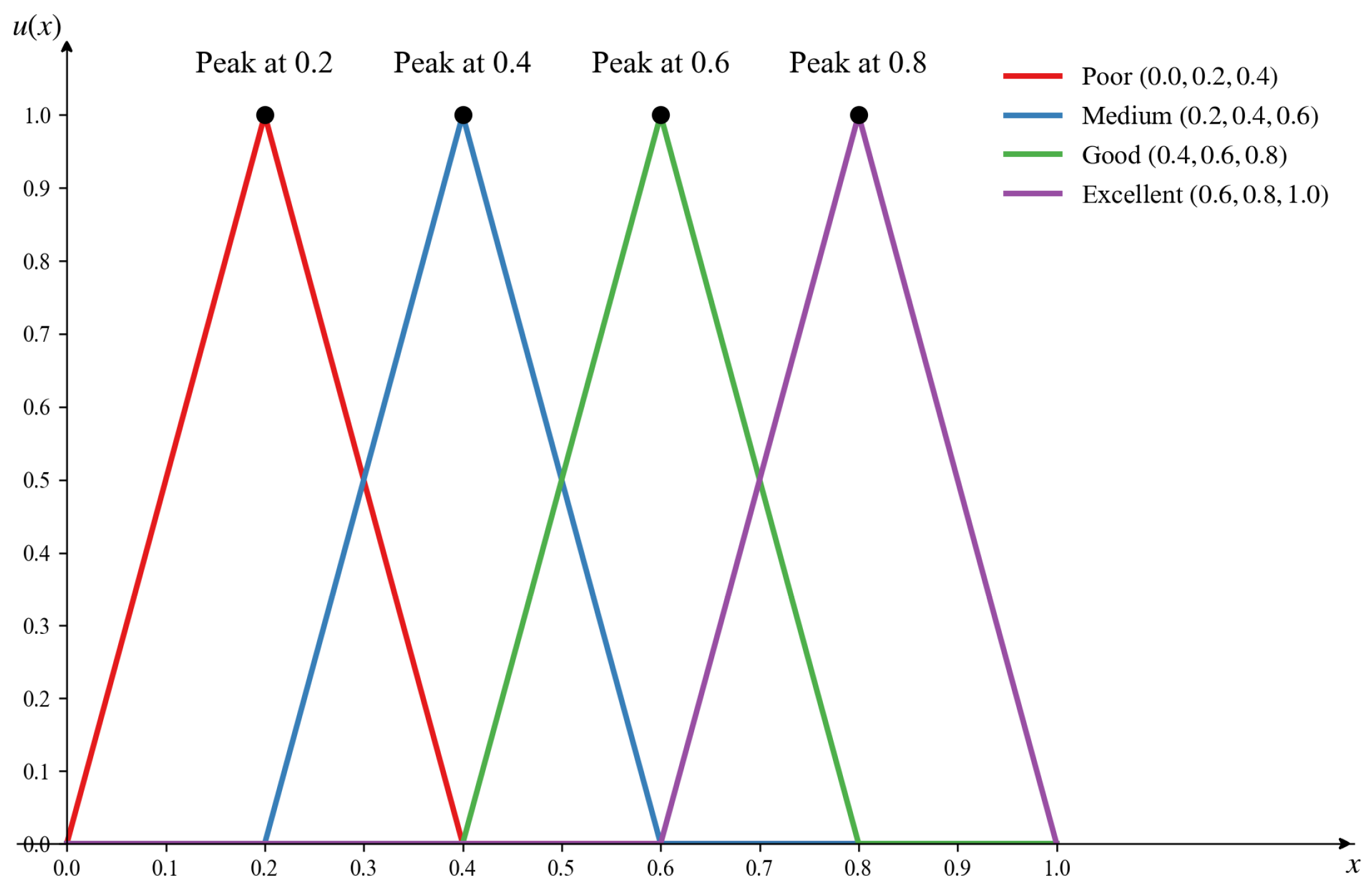
The battlefield environment is one of the critical factors affecting the performance of combat effectiveness. Given its significant complexity, it is challenging to describe the battlefield environment using precise numerical values. However, during specific combat operations, factors such as combat location and meteorological conditions tend to remain relatively stable, allowing for the determination of a relative range for the environmental condition attribute. Consequently, the battlefield environment condition can be categorized into four levels: excellent, good, medium, and poor. To quantify the inherent uncertainty in these environmental indicators, triangular fuzzy numbers are employed. The membership function for environmental threat is established, as depicted in Figure 7. When the environmental condition corresponds to the poor level, the corresponding mathematical expression is provided below, with analogous expressions applicable to the other levels.
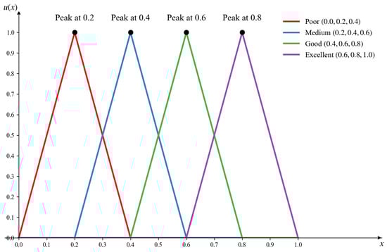
Figure 7.
Environment threat function.
Target Intention
Let the intention space of the UAV be represented as . In this study, the dimension L of the intention space is set to 6, corresponding to the following intentions: attack, retreat, electronic jamming, surveillance, reconnaissance, and feint attack. The matrix consisting of the probabilities of each target under each intention is referred to as the intention probability matrix, denoted as , which can be expanded as follows:
where , , denotes the probability that the i-th target belongs to the j-th intention, as derived from the results of UAV intention recognition.
3.1.3. Transforming Heterogeneous Indexes into a Unified IFS
The above-mentioned attributes exhibit substantial discrepancies in data types and dimensions. To address this, it is essential to transform heterogeneous information into a unified IFS format, thereby eliminating discrepancies among multi-source data and constructing an intuitionistic fuzzy decision matrix for subsequent dynamic weight calculation and threat prioritization.
- 1.
- Transformation of Fuzzy Evaluation Language into IFS
The conversion relationship between the fuzzy evaluation language scale and intuitionistic fuzzy numbers is presented in Table 3, while Table 4 illustrates the interval value relationships corresponding to the decision-maker’s degree of certainty regarding their judgments.
Table 3.
Scale of fuzzy evaluation language and transformation to IFN.
Table 4.
Determination degree corresponding to interval values.
- Step 1: Based on the information provided in Table 3 and Table 4, the i-th fuzzy evaluation language can be represented as follows:where , , and denote the intuitionistic fuzzy number corresponding to the fuzzy evaluation language scale and represents the interval number reflecting the degree of certainty of the fuzzy evaluation language .
- Step 2: Based on Equation (18), the fuzzy evaluation language can be transformed into an intuitionistic fuzzy number .where denotes the intuitionistic fuzzy number associated with the intermediate scale , while indicates the decision-maker’s level of certainty regarding their decision. The function of is to ensure that the decision result converges toward the intermediate decision value as the decision-maker’s degree of certainty diminishes.
- 2.
- Transformation of interval numbers into IFS
Attributes represented by interval numbers can be categorized into benefit and cost types. In this study, all quantified attributes belong to the benefit type and are transformed according to Equation (19).
- 3.
- Transformation of real numbers into IFS
Real numbers can be considered as a special case of interval numbers, and the membership degree and non-membership degree of the target angle threat degree can be calculated using Equation (20).
where is an additional fuzzy factor introduced to prevent the deterministic nature of real numbers from influencing other uncertainty indicators. In this study, it is set to 0.8.
- 4.
- Transformation of triangular fuzzy numbers into IFS
For the triangular fuzzy number , , its membership function can be expressed as follows:
The triangular fuzzy number can be transformed into an intuitionistic fuzzy number using Formula (22).
After the aforementioned calculations, all attribute data obtained at are converted into IFS to construct an intuitionistic fuzzy evaluation matrix ,, which serves as the basis for subsequent computations.
3.2. Weight Determination Method of Indexes
3.2.1. Determination of Time Series Weight
The results of target threat assessment are heavily influenced by the information about the current situation. Typically, the closer the situational information is to the current moment, the greater its contribution to the assessment. Consequently, this paper employs the inverse Poisson distribution method to determine the weights of the time series. The detailed calculation steps are presented as follows:
where the value of typically falls within the range of and is generally set to 1.5 [28].
3.2.2. Determination of Objective Weight Based on IFE
Information entropy can effectively reflect the characteristics of fuzzy data. A higher information entropy indicates that the information provided by an attribute is more uncertain, which in turn reduces the validity of the evaluation data and decreases the attribute weight. Therefore, this paper determines the objective weights of the target attributes by calculating the cosine IFE. By integrating the evaluation matrix at each moment with the time series weight obtained from Formula (23) and performing calculations according to Formula (10), the time series-weighted matrix can be derived:
The detailed calculation procedure for the IFE of each attribute is presented as follows:
- Step 1: Calculating the cosine intuitionistic fuzzy entropy of each attribute based on Equation (26).where denotes the intuitionistic fuzzy entropy of the j-th attribute, while indicates the hesitation degree of the IFS, and its calculation is presented in Equation (4).
- Step 2: Constructing a quadratic nonlinear programming model, with the minimization of IFE serving as the objective function, as presented in Equation (27).
- Step 3: Establishing the Lagrange equation to solve Equation (27).
- Step 4: By taking the derivatives of and in Equation (28), the objective weight of the j-th attribute is obtained by Equation (30).
3.2.3. Determination of Subjective Weight Based on AHP and Target Intention
The combat intentions of air targets are dynamically changeable. Under different combat scenarios, the significance of each attribute varies. In military operations, commanders serve as the decision-making core of the army. Hence, this paper leverages the combat experience of commanders to comparatively evaluate the significance and quantitatively determine the weight of each attribute. The specific steps for calculating the subjective weight fusing intention probability matrix based on the AHP method are as follows:
- Step 1: Constructing the model of the AHP based on the index system for UAV threat assessment, as illustrated in Figure 8.
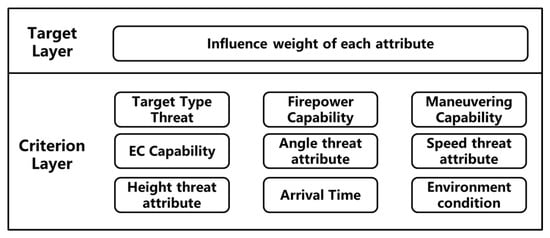 Figure 8. Analytic hierarchy process model diagram.
 - Step 2: Constructing the judgment matrix. The 9-level ratio scale method is employed to perform pairwise comparisons of the attributes and construct the judgment matrix . The evaluation criteria consist of equally important (1), slightly important (3), noticeably important (5), strongly important (7), and extremely important (9) in the 9-level scale. Intermediate values between adjacent scales are represented by 2, 4, 6, and 8.
- Step 3: Calculating the weight vector. The eigenvector method is employed to determine the weight of each judgment matrix.
- (1)
- Solving Equation (31) to compute the maximum eigenvalue .
- (2)
- Solving Equation (32) yields the non-zero eigenvector w.
- (3)
- Normalizing the eigenvector into a weight vector using Equation (33).
- Step 4: Performing a consistency check.
- (1)
- Calculating the consistency index (CI) using Equation (34):
- (2)
- Querying the random consistency index (RI), RI = [0, 0, 0.52, 0.89, 1.12, 1.26, 1.36, 1.41, 1.46, 0.49, 0.52, 1.54, 1.56, 1.58, 1.59].
- (3)
- Calculating the consistency ratio (CR), . If CR < 0.1, the test is passed; otherwise, the judgment matrix needs to be adjusted.
- Step 5: Repeating Steps 2~4 to calculate the weights of each attribute for the six combat intention types and constructing the combat intention attribute weight matrix (35).where denotes the weight of the j-th attribute under the i-th intention, and it satisfies .
- Step 6: Calculating the subjective weights of each attribute. By using matrix (35) and the intention probability matrix (16), the subjective weight matrix can be obtained, and the calculation is as follows:where represents the subjective weight of the j-th attribute for the i-th target.
3.2.4. Determination of Comprehensive Variable Weight Based on the Least Squares Method
To balance expert experience and data information, a least squares method for fusing subjective and objective weights by considering IFS scores was developed. The core principle of IFS scores lies in quantifying the certainty and importance of attributes, enabling dynamic adjustment of the deviation between subjective and objective weights, and thus achieving scientifically integrated results. The specific steps are as follows.
- Step 1: Calculating the IFS scores for each attribute. The calculation equation for the score of the j-th attribute under the i-th target is presented in (37).
- Step 2: Repeating Step 1 to construct the score matrix for the weighted intuitionistic fuzzy evaluation matrix , as presented in (38).
- Step 3: Defining the weighted decision-making bias by using Equation (39).
- Step 4: Developing a least squares weight fusion model based on minimizing the total decision deviation, as presented in (40).where J represents the total decision-making deviation, and is the preference factor between the objective weight and the subjective weight. is a given positive number, which is set according to the actual situation. In this paper, , .
- Step 5: Solving (40), the comprehensive variable weight for the i-th target is obtained.
- Step 6: By repeating Steps 3~5, the comprehensive variable weight matrix for multiple objectives is obtained, as shown in (41).
3.3. Threat Degree Ranking Based on the Improved TOPSIS Method
By integrating the time series-weighted matrix with the comprehensive variable weight matrix W, the ranking is performed using the improved TOPSIS method. The detailed steps are presented below:
- Step 1: Obtaining the relative positive ideal solution and the relative negative ideal solution of the threat assessment attributes. The process for calculating and of each attribute is presented below.where denotes the set of benefit-type indicators, represents the set of cost-type indicators, and .
- Step 2: Calculating the hesitation degrees and relative to the positive ideal solution and the negative ideal solution of each evaluation attribute , where ,, and , .
- Step 3: Calculating the degree of similarity and between the corresponding to each attribute of each target and the relative positive ideal solution and the relative negative ideal solution , respectively, thereby constructing the positive similarity degree matrix and the negative similarity degree matrix . The calculation process for the positive similarity degree is presented in Equation (44), while the process for the negative similarity degree is shown in Equation (45).where . m denotes the total number of targets, while n indicates the total number of threat assessment attributes for UAVs, and , .
- Step 4: Based on the comprehensive variable weight matrix W, the weighted positive scores and weighted negative scores for each target are calculated, respectively, using Equations (46) and (47).where and denote the comprehensive variable weight of the j-th attribute for the i-th target, and , , , and is satisfied.
- Step 5: Calculating the relative degree of closeness for each target .where and . The larger the value of , the higher the threat level of the corresponding target , and the more prioritized its ranking in the threat assessment.
4. Simulation and Analysis
4.1. Simulation Example
In the experimental design section, we selected five UAV targets and three time points to simulate realistic scenarios commonly encountered in military environments. This configuration aligns with the experimental designs presented in numerous related studies [12,18]. By employing this simplified model, we are able to concentrate on the essential aspects of the decision-making process while ensuring that the experimental results remain highly interpretable and practically relevant.
In an air defense operation, five types of air attack targets performed strikes or reconnaissance against the defended asset. Based on the established UAV threat assessment index system, the raw data of the targets at a specific moment, obtained through battlefield reconnaissance, detection, and tracking, are presented in Table 5, Table 6, Table 7 and Table 8. The results of UAV intention recognition, acquired via the command and control system, are shown in Table 9. The experiments were conducted using MATLAB R2024a on a personal computer equipped with an Intel Core i7-9700 CPU operating at 3.60 GHz and with 16 GB of RAM (Intel Corporation, Santa Clara, CA, USA). The system was running a Windows 10 (x86-64) operating system.
Table 5.
Original inherent data information of multi-targets.
Table 6.
Original situation data information of multi-targets at t1.
Table 7.
Original situation data information of multi-targets at t2.
Table 8.
Original situation data information of multi-targets at t3.
Table 9.
Target intention information.
The nine threat attributes, including target type threat, firepower capability, maneuvering capability, electronic countermeasure capability, angle threat, speed threat, height threat, arrival time threat, and environmental conditions, are defined as . Based on the raw target data presented in Table 5, Table 6, Table 7 and Table 8, the threat assessment model illustrated in Figure 1, and the algorithm flow outlined in Algorithm 1, the following steps were conducted for target threat assessment:
- Step 1: Based on Section 3.1.2, the data presented in Table 5, Table 6, Table 7 and Table 8 were quantified to derive the corresponding threat values, which are illustrated in Table 10, Table 11, Table 12 and Table 13.
Table 10. Quantified inherent data information of multi-targets.
Table 11. Quantified situation data information of multi-targets at t1.
Table 12. Quantified situation data information of multi-targets at t2.
Table 13. Quantified situation data information of multi-targets at t3.
- Step 2: According to Section 3.1.3, heterogeneous information was transformed into the same IFS form to form the intuitionistic fuzzy decision matrix , at each moment:
- Step 3: According to Equation (23), the time series weight at each moment K was calculated. Subsequently, by integrating the evaluation matrix at each moment with Equation (10), the time series-weighted matrix was obtained.
- Step 4: The objective weight vector was calculated according to Equations (26)–(30).
- Step 5: By utilizing the data in Table 8, the intention probability matrix was constructed. Subsequently, based on Equations (31)–(36), the weight matrix of combat intention indicators and the subjective weight matrix were calculated.
- Step 6: By integrating the objective weight vector and the subjective weight matrix , the comprehensive variable weight matrix for multi-targets was calculated based on Equations (37)–(40).
- Step 7: By integrating the time series-weighted matrix with the comprehensive variable weight matrix W and applying the improved TOPSIS method for ranking, the relative closeness degrees of the targets and their corresponding threat rankings were derived, as presented in Table 14.
Table 14. The threat ranking results of the proposed model.
4.2. Comparison Analysis
- 1.
- Model 1 [18]: intuitionistic fuzzy TOPSIS method without fuse intention
If the threat assessment method does not integrate intention, it will be similar to the model presented in Reference [18]. The specific calculation steps are outlined as follows:
- Step 1~Step 4: In line with the proposed model, the resulting objective weights are presented as follows:
- Step 5: By integrating the time series-weighted matrix with the comprehensive variable weight matrix W, and applying the improved TOPSIS method for ranking, the relative closeness degrees of the targets and their corresponding threat rankings were derived, as presented in Table 15.
Table 15. The threat ranking results of Model 1.
- 2.
- Model 2 [12]: intuitionistic fuzzy TOPSIS method with single moment
If the threat assessment method fails to integrate information from multiple time points and instead evaluates solely based on single-moment information, it will be analogous to the model presented in [12]. The detailed calculation steps are outlined as follows:
- Step 1~Step 2: In accordance with the proposed model, the intuitionistic fuzzy decision matrix at time t3 was derived:
- Step 3: The objective weight vector was calculated based on Equations (26)–(30):
- Step 4: The subjective weight matrix was calculated according to Equations (31)–(36):
- Step 5: The objective weight vector and the subjective weight matrix were combined, and the comprehensive variable weight matrix of multiple targets was obtained according to Equations (37)–(40):
- Step 6: By integrating the intuitionistic fuzzy matrix with the comprehensive variable weight matrix W, and applying the improved TOPSIS method for ranking, the relative closeness degree of the target and the threat ranking were determined, as presented in Table 16.
Table 16. The threat ranking results of Model 2.
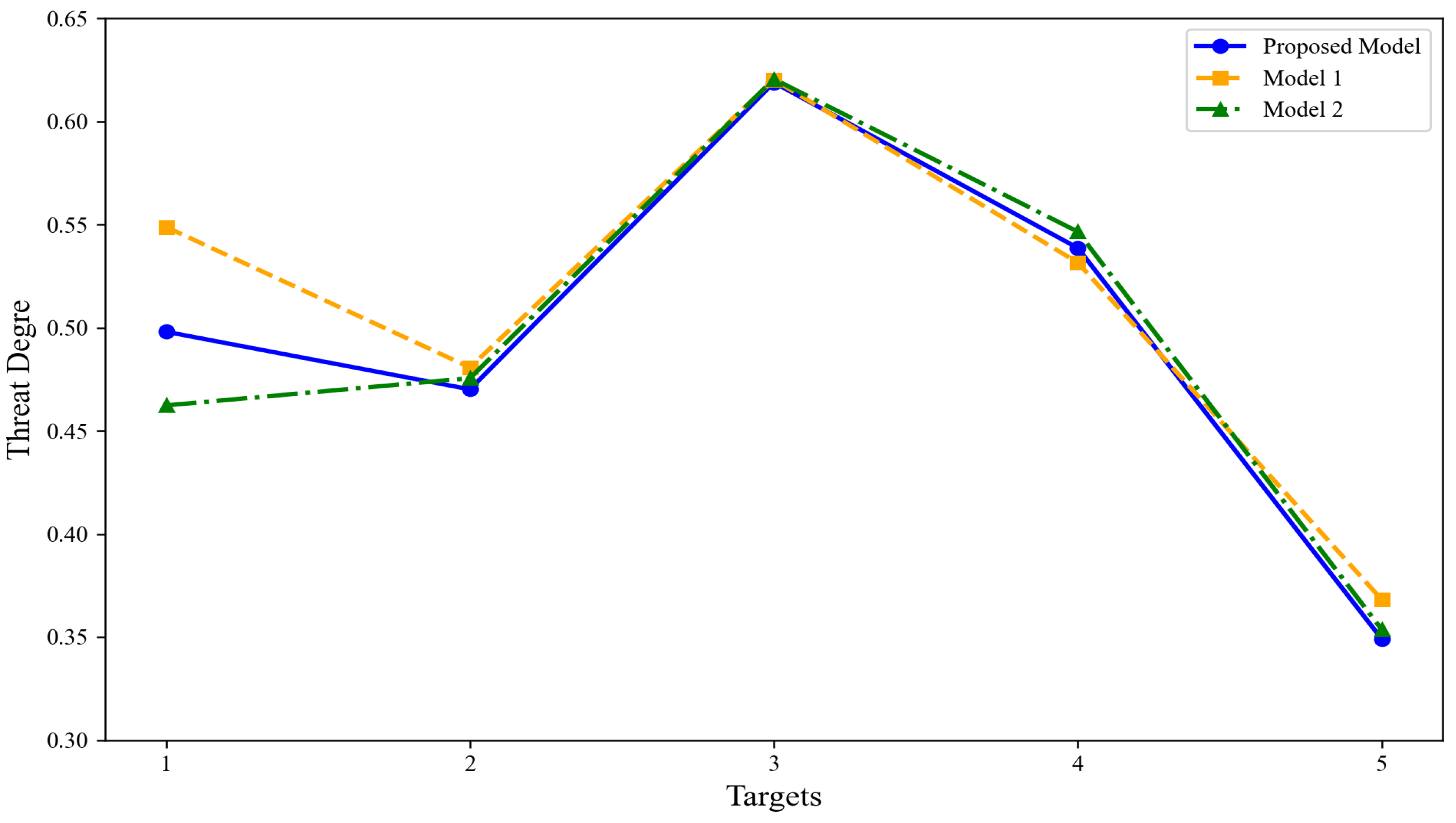
The threat degrees obtained using the model proposed in this paper were compared with Model 1 and Model 2 as described earlier, with the results presented in Figure 9 and Figure 10. From these figures, it can be observed that all three models successfully identify as the target with the highest threat degree and as the target with the lowest threat degree. However, discrepancies exist in the threat assessment rankings of targets , , and . Compared to the proposed model, Model 1 does not account for the target’s intention during the evaluation process, leading to the conclusion that the threat posed by target is higher than that of target . Nevertheless, at the latest moment, there is a 58% probability that the intention of target is “retreat,” whereas target has a 62% probability of being “attack.” Clearly, target should exhibit a higher threat degree than the other target. In contrast to the proposed model, Model 2 fails to incorporate data fusion across multiple time points, relying solely on single-moment data for assessment, which results in the conclusion that the threat of target is greater than that of target . However, when combining data from time point and , it becomes evident that target exhibits a higher threat degree than target at both and . The essence of threat assessment lies in evaluating the continuous impact of a target on battlefield dynamics. Target consistently demonstrates a threat advantage over target during early moments, indicating stronger stability and continuity in its threat profile, along with a more significant cumulative threat effect. Consequently, the potential threat posed by target remains greater than that of target and is more likely to exert long-term influence on the battlefield. Therefore, it is reasonable to conclude that the threat degree of target is greater.
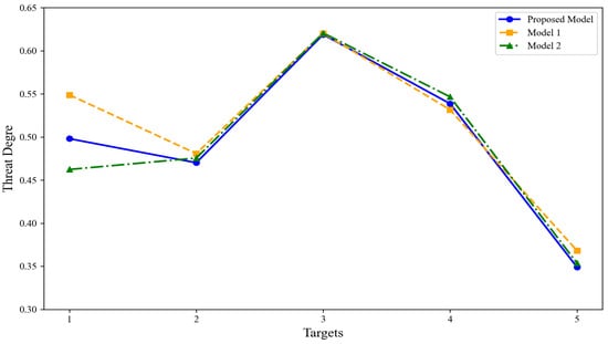
Figure 9.
Comparison of target threat assessment results of three models.

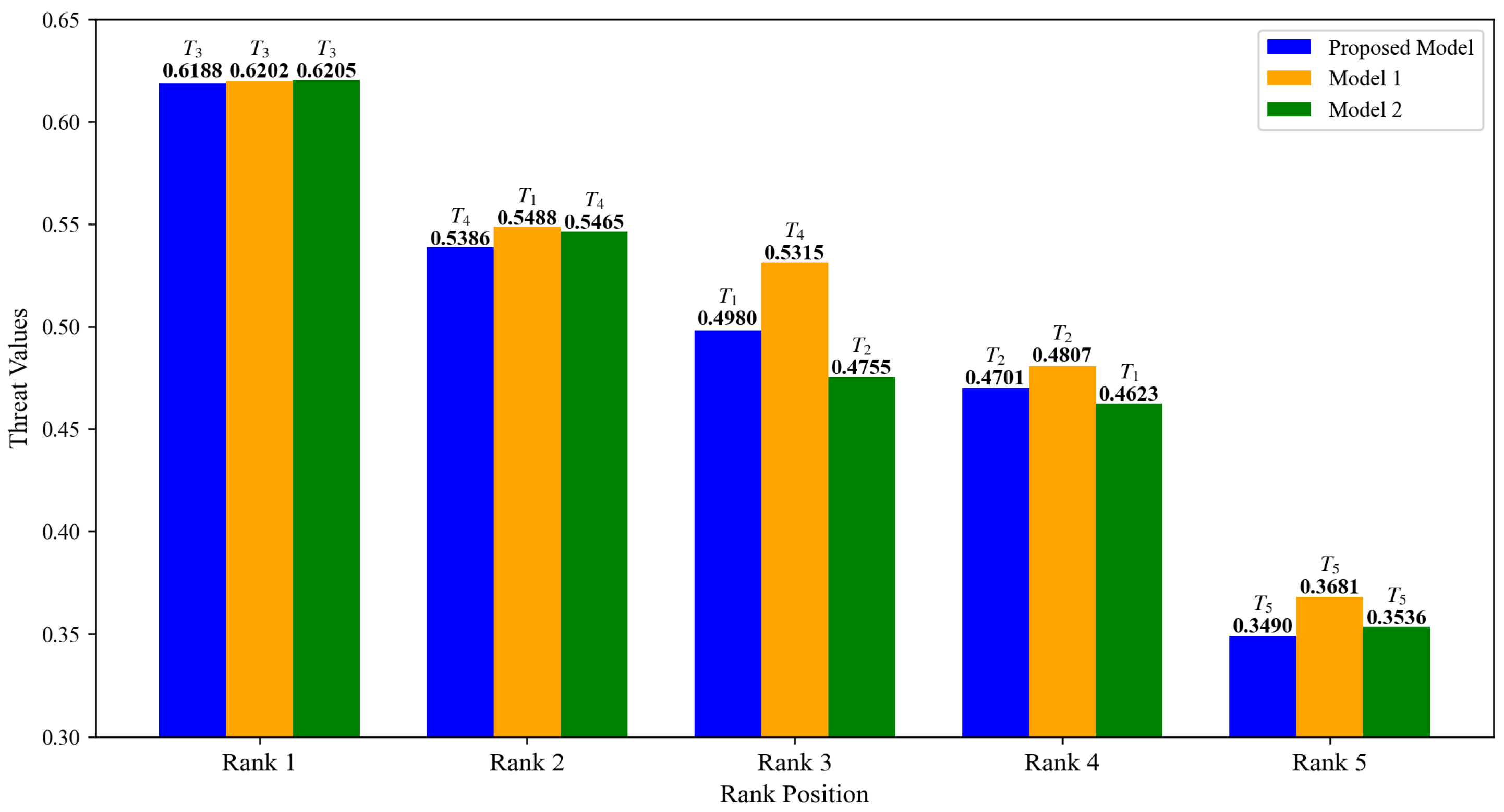
Figure 10.
Comparison of target threat ranking of three models.
Furthermore, analyzing the bar charts in Figure 10 reveals that the threat degrees of the five targets obtained by Model 1, which neglects target intention fusion, are universally higher than the proposed model and Model 2 (which does not integrate multi-time data). We hold that the inflated threat levels in Model 1 arise because it does not dynamically adjust the weights of attributes according to the target’s varying intentions, resulting in an unreasonable assessment. Conversely, models that incorporate the target’s intentions can effectively align with the dynamic nature of the target, fully leverage available information, and produce more accurate and reliable threat level results.
5. Conclusions
Aiming at the threat assessment problem of UAVs in battlefield environments, this paper proposes a dynamic multi-target and multi-time threat assessment method for UAVs based on fuzzy multi-attribute decision making and intention fusion. Firstly, by constructing an effective UAV threat assessment index system, the required attribute data from sensors are extracted and represented in heterogeneous forms. After attribute quantification and unified transformation, an intuitionistic fuzzy evaluation matrix is obtained. Through time-weighted processing, a comprehensive evaluation matrix is derived. On this basis, objective weights are calculated using the cosine intuitionistic fuzzy entropy method, while subjective weights are determined by fusing the probability matrix of intentions to effectively integrate target combat intention information. Simultaneously, a comprehensive variable weight fusion method considering IFS scores is designed to distinguish the comprehensive weights of multiple targets. Finally, the TOPSIS method based on hesitation degree weighted similarity measurement, which is more suitable for the intuitionistic fuzzy environment, is employed to derive the threat ranking of the targets. Simulation analysis and comparative experiments demonstrate that this method can comprehensively consider the capability, opportunity, and intention of multiple UAV targets, accurately providing threat assessment results through multi-time situational information. The proposed approach for UAV threat assessment is directly applicable to real-time military decision support systems. In dynamic and uncertain battlefield environments, commanders are required to rapidly prioritize responses to multiple UAV threats while accounting for incomplete or ambiguous information [9]. Similar applications of fuzzy logic in military systems have demonstrated improved reliability and adaptability in uncertain environments [29]. However, the research presented in this paper has certain limitations: when the expert knowledge base established for each intention is incomplete, the reliability of the evaluation decreases. Moreover, the current model may introduce computational challenges when handling large-scale data. Future work will primarily focus on three key areas: (1) expanding the set of threat assessment attributes to enhance comprehensiveness; (2) further refining the structure of the threat assessment attribute quantification function for improved accuracy; and (3) integrating parallel and distributed computing frameworks while employing incremental computation techniques. This combination will enable dynamic updates of threat assessments in time series data analysis, thereby accelerating complex computations in large-scale data processing.
Author Contributions
Conceptualization, Q.N. and S.R.; methodology, Q.N. and S.R.; software, validation, formal analysis, Q.N.; writing—original draft preparation, Q.N.; writing—review and editing, Q.N. and W.G. and C.W.; supervision, project administration, C.W. All authors have read and agreed to the published version of the manuscript.
Funding
This research received no external funding.
Data Availability Statement
The original contributions presented in this study are included in the article. Further inquiries can be directed to the corresponding author.
Conflicts of Interest
The authors declare no conflicts of interest.
Abbreviations
The following abbreviations are used in this manuscript:
| UAVs | Unmanned aerial vehicles |
| TOPSIS | Technique for order preference by similarity to ideal solution |
| MADM | Multi-attribute decision making |
| IFS | Intuitionistic fuzzy set |
| IFN | Intuitionistic fuzzy number |
| IFWA | Intuitionistic fuzzy weighted averaging |
| IFMADM | Fuzzy multi-attribute decision making |
| AHP | Analytic hierarchy process |
| IF-AHP | Intuitionistic fuzzy analytic hierarchy process |
| GIFSS | Generalized intuitionistic fuzzy soft set |
References
- Benavoli, A.; Ristic, B.; Farina, A.; Oxenham, M.; Chisci, L. An approach to threat assessment based on evidential networks. In Proceedings of the 2007 10th International Conference on Information Fusion, Quebec, QC, Canada, 9–12 July 2007; pp. 1–8. [Google Scholar]
- Wang, Y.; Liu, S.; Niu, W.; Liu, K.; Liao, Y. Threat assessment method based on intuitionistic fuzzy similarity measurement reasoning with orientation. China Commun. 2014, 11, 119–128. [Google Scholar]
- Fan, C.; Fu, Q.; Song, Y.; Lu, Y.; Li, W.; Zhu, X. A new model of interval-valued intuitionistic fuzzy weighted operators and their application in dynamic fusion target threat assessment. Entropy 2022, 24, 1825. [Google Scholar] [CrossRef] [PubMed]
- Di, R.; Gao, X.; Guo, Z.; Wan, K. A threat assessment method for unmanned aerial vehicle based on bayesian networks under the condition of small data sets. Math. Probl. Eng. 2018, 2018, 8484358. [Google Scholar] [CrossRef]
- Zhang, K.; Kong, W.; Liu, P.; Shi, L.; Lei, Y.; Zou, J. Assessment and sequencing of air target threat based on intuitionistic fuzzy entropy and dynamic VIKOR. J. Syst. Eng. Electron. 2018, 29, 305–310. [Google Scholar] [CrossRef]
- Qu, C.; He, Y.; Ma, Q. Threat Assessment Using Multiple Attribute Decision Making. Syst. Eng. Electron. 2000, 22, 26–29. [Google Scholar]
- Ma, S.; Zhang, H.; Yang, G. Target threat level assessment based on cloud model under fuzzy and uncertain conditions in air combat simulation. Aerosp. Sci. Technol. 2017, 67, 49–53. [Google Scholar] [CrossRef]
- Yu, X.; Wei, S.; Fang, Y.; Sheng, J.; Zhang, L. Low-altitude slow small target threat assessment algorithm by exploiting sequential multifeature with long short-term memory. IEEE Sens. J. 2023, 23, 21524–21533. [Google Scholar] [CrossRef]
- Song, Y.; Luo, Z.; Huang, J.; Shi, J. Progress in Military Target Threat Assessment. Syst. Eng. Electron. 2025, 1–23. Available online: https://link.cnki.net/urlid/11.2422.tn.20250305.1103.006 (accessed on 16 April 2025).
- Atanassov, K.T. Intuitionistic fuzzy sets. Fuzzy Sets Syst. 1986, 20, 87–96. [Google Scholar] [CrossRef]
- Xiao, L.; Qi, H.; Qu, J. Air target threat assessment based on intuitionistic fuzzy analytic hierarchy process. J. Detec. Contr 2019, 41, 108–111. [Google Scholar]
- Qi, C.; Sun, J.; Wang, Y.; Cai, P.; Rong, X. Threat comprehensive assessment for air defense targets based on intuitionistic fuzzy TOPSIS and variable weight VIKOR. Syst. Eng. Electron. 2022, 4, 172–180. [Google Scholar]
- Xu, Z.; Yager, R.R. Dynamic intuitionistic fuzzy multi-attribute decision making. Int. J. Approx. Reason. 2008, 48, 246–262. [Google Scholar] [CrossRef]
- Huang, J.; Li, B.; Zhao, Y. Application of Intuitive Fuzzy Sets Choquet Integral in Target Threat Assessment. J. Inf. Eng. Univ. 2014, 15, 6–11. [Google Scholar]
- Azimirad, E.; Haddadnia, J. Target threat assessment using fuzzy sets theory. Int. J. Adv. Intell. Inform. 2015, 1, 57–74. [Google Scholar] [CrossRef]
- Zhang, K.; Wang, X.; Zhang, C.K.; Zhou, D.Y.; Feng, Q. Evaluating and sequencing of air target threat based on IFE and dynamic intuitionistic fuzzy sets. Syst. Eng. Electron. 2014, 36, 697–701. [Google Scholar]
- Feng, J.; Zhang, Q.; Hu, J.; Liu, A. Dynamic assessment method of air target threat based on improved GIFSS. J. Syst. Eng. Electron. 2019, 30, 525–534. [Google Scholar] [CrossRef]
- Gao, Y.; Li, D.; Zhong, H. A novel target threat assessment method based on three-way decisions under intuitionistic fuzzy multi-attribute decision making environment. Eng. Appl. Artif. Intell. 2020, 87, 103276. [Google Scholar] [CrossRef]
- Fu, T.; Wang, J. Threat Assessment of Aerial Targets in Air-Defense. Command. Control. Simul. 2016, 3, 63–69. [Google Scholar]
- Li, Z.; Wang, S.; Chai, H.; Xu, Q. Spatial Target Threat Assessment Based on the Combination of AHP and Entropy Weight Method. J. Inf. Eng. Univ. 2024, 25, 751–756. [Google Scholar]
- Zadeh, L.A. Fuzzy sets. Inf. Control 1965, 8, 338–353. [Google Scholar] [CrossRef]
- Atanassov, K.T. More on intuitionistic fuzzy sets. Fuzzy Sets Syst. 1989, 33, 37–45. [Google Scholar] [CrossRef]
- Xu, Z. Intuitionistic fuzzy aggregation operators. IEEE Trans. Fuzzy Syst. 2007, 15, 1179–1187. [Google Scholar]
- Kumar, K.; Chen, S. Multiattribute decision making based on q-rung orthopair fuzzy Yager prioritized weighted arithmetic aggregation operator of q-rung orthopair fuzzy numbers. Inf. Sci. 2024, 657, 119984. [Google Scholar] [CrossRef]
- Ranjbar, H.R.; Nekooie, M.A. An improved hierarchical fuzzy TOPSIS approach to identify endangered earthquake-induced buildings. Eng. Appl. Artif. Intell. 2018, 76, 21–39. [Google Scholar] [CrossRef]
- Çalı, S.; Balaman, Ş.Y. A novel outranking based multi criteria group decision making methodology integrating ELECTRE and VIKOR under intuitionistic fuzzy environment. Expert Syst. Appl. 2019, 119, 36–50. [Google Scholar] [CrossRef]
- Yoon, K.P.; Hwang, C. Multiple Attribute Decision Making: An Introduction; Sage Publications: New York, NY, USA, 1995. [Google Scholar]
- Pires, H.B.; Guimarães, L.N.F. Dynamic Multi-Target Three-Way Threat Assessment in the Context of Air Defense. IEEE Access 2024, 12, 141397–141413. [Google Scholar] [CrossRef]
- Coskun, M.; Tasdemir, S. Fuzzy Logic-Based Threat Assessment Application in Air Defense Systems. IEEE Trans. Aeros Electron. Syst. 2023, 59, 2245–2251. [Google Scholar] [CrossRef]
Disclaimer/Publisher’s Note: The statements, opinions and data contained in all publications are solely those of the individual author(s) and contributor(s) and not of MDPI and/or the editor(s). MDPI and/or the editor(s) disclaim responsibility for any injury to people or property resulting from any ideas, methods, instructions or products referred to in the content. |
© 2025 by the authors. Licensee MDPI, Basel, Switzerland. This article is an open access article distributed under the terms and conditions of the Creative Commons Attribution (CC BY) license (https://creativecommons.org/licenses/by/4.0/).