End-to-End Predictive Network for Accurate Early Crop Planting Area Estimation

Abstract

Early crop planting area estimation is crucial for achieving effective government resource allocation, optimizing resource distribution planning, and preparation related to food security. Utilizing remote sensing images during the crop growth period for crop planting area estimation has garnered increasing attention. However, area estimation from remote sensing often lags in obtaining image data. Moreover, this method is also influenced by the quality of remote sensing image data and segmentation accuracy. This paper proposes a new method for early area estimation based on multi-year land cover data using a three-dimensional convolutional end-to-end network. This method eliminates the impact of the intermediate process of image segmentation accuracy on area estimation. Additionally, multi-subimage technology is employed to solve the issue of inconsistent input sample size, and label distribution smoothing technology is used to tackle the problem of unbalanced sample distribution. The proposed method was evaluated on U.S. corn and soybean datasets. In comparison to baseline methods, the method achieved relative errors of 0.67% for corn and 3.72% for soybeans at the national level in the United States in 2021. This demonstrates the effectiveness of the proposed method and the potential for early decision-making support. This approach offers a new perspective for area estimation, significantly advancing the timing of planting area prediction and enhancing the accuracy of early area estimation, providing actionable insights for decision-making and resource management.

1. Introduction

The early estimation of crop planting areas [1] aims to predict the crop planting areas in specific regions. Against the international backdrop of frequent extreme weather events, escalating global conflicts, and intensifying economic shocks, food production and supply chain trade are severely threatened, and the importance of food security has become even more prominent [2,3,4,5]. Accurate and timely agricultural production information is crucial for ensuring global food security [6]. As a key link in achieving the effective allocation of government resources, optimizing resource allocation plans and preparations, and formulating import and export strategies related to food security, accurate and timely information on the early estimation of crop planting areas is of great significance for ensuring global food security [7].

With the development of space satellite technology, the estimation of crop planting areas has shifted from labor-intensive methods (such as manual interviews and field surveys) to a traditional approach with remote sensing image processing. This method has become the mainstream approach for estimating large-scale planting areas because it can effectively monitor large areas of land and reduce the reliance on physical labor. It involves two main steps: first, classifying remote sensing images [8,9,10], and then calculating the planting area based on the classification results [11].

This method is limited by remote sensing datasets and the shortcomings of the traditional model, often falling short in high-precision crop area estimation. First, the timing of remote sensing image acquisition and crop germination characteristics limit the availability of images during the early stages of crop growth, resulting in delays in area estimation [12,13]. Second, for the traditional method, the errors arise from both the imperfect classification or segmentation results (e.g., commission, omission) and the limitations of the subsequent area calculation stage (e.g., handling mixed pixels, boundary effects, and the spatial resolution limitations of remote sensing images) [12,14,15,16]. All of the above are the key difficulties that are currently hard to overcome in area estimation work.

In addition, during the estimation of the planting area, there is also a problem of a lack of consistency in different sample inputs. For deep learning models, the unevenness of input sizes can easily plunge the models into training difficulties. In the realm of traditional visual computing, conventional means such as scaling and cropping are generally used to process data. However, since the model input data carry actual geographical information and are restricted by practical factors such as the shapes and sizes of administrative regions, traditional image processing techniques are not applicable in this context, thus adding numerous difficulties to the estimation of the planting area.

Last but not least, the labeled data of the planting area exhibit a markedly uneven distribution. Taking the planting area data at the county level in the United States as an example, influenced by multiple factors including local climate conditions and geographical environment, the data distribution among various county-level units varies greatly and is extremely uneven [17]. This imbalance further exacerbates the difficulty of training deep models.

In this study, the primary motivation and contribution of our approach lie in the early prediction of time. We propose an end-to-end predictive network for an accurate early crop planting area estimation method. This method utilizes the land cover data accumulated over the past several years to predict the planting area of the current year. Theoretically, once the crops are harvested in the previous year, the planting area for the next year can be calculated accordingly. The proposed method is evaluated on county-level corn and soybean planting area estimation in the United States, and the experimental results show the effectiveness of the model.

The contributions of this work are as follows:

• We propose a novel large-scale end-to-end method for early estimation of crop planting areas that avoids the errors of traditional methods as much as possible and completes the prediction before the crops are sown. Moreover, the end-to-end predictive network has potential in capturing complex spatiotemporal dependencies.
• A time-series-based pixel inference method is proposed. Land cover datasets from previous years are used as the data source, instead of relying on remote sensing images from the current year, which addresses data scarcity in early planting area estimation.
• A multi-subimage technique is proposed to effectively resolve the challenge of uneven input sizes in remote sensing images for end-to-end model training. Additionally, a label distribution smoothing technique alleviates data imbalance in crop planting predictions.

2. Related Work

Crop planting area estimation aims to predict the area of a specific crop in a given region. For example, Door County has a soybean planting area of 21,500 acres, and Brown County has a soybean planting area of 13,600 acres, estimated from remote sensing data, shown in Figure 1.

For region $n$ in year $y$, we assume the availability of earth observation data $d_{n,y}ϵR^{H\times W}$ and corresponding specific crop planting area data $a_{n,y}ϵR$, where $H$ and $W$ denote the spatial resolution (height and width) of the data $d$. Let $D=\left\{d_{n,y}\right\}$ and $A=\left\{a_{n,y}\right\}$. We aim to develop a function F(⋅) that maps the input data $D$ to the planting area $A$, capturing the relationship between the spatial features and the crop planting area.

$$F\left(D\right)=A$$

(1)

Currently, area estimation typically employs the two-stage approach to solve the problem $F\left(D\right)=\mathrm{A}$ of classification and area estimation.

In the crop planting area segmentation stage, previous related works have primarily relied on remote sensing images, making the accuracy of crop area extraction heavily dependent on the quality of these images [18]. Bellon et al. [11] addressed the impact of cloud cover on crop area segmentation by combining remote sensing images with various vegetation indices. Several studies [19,20,21,22,23,24,25] have demonstrated the effectiveness of deep learning in handling complex datasets. For example, Gallo et al. [22] proposed a 3D-FPN network utilizing time-series remote sensing images. This method employs a three-dimensional pyramid convolutional neural network to integrate temporal and spatial features of remote sensing data, achieving accurate crop area segmentation. Leveraging temporal complementarity mitigates the impact of low-quality images. Building on this, Yan and Yang et al. [24,25] extended the approach to multi-source satellite datasets, further improving classification performance. Wang et al. [26] proposed a Temporal Memory Attention Network (TMANet) based on the self-attention mechanism, which is capable of adaptively integrating temporal relationships in time series data. Specifically, this method constructs a memory using images from several previous moments to store the temporal information of the current image. On this basis, the researchers further designed a Temporal Memory Attention Module to capture the relationship between the current frame and the memory, thereby enhancing the representation of the current image. Through this approach, the network can achieve pixel-level image classification. However, there are still misclassification and missed classification phenomena in the classification and segmentation results of the above-mentioned methods.

In the crop planting area calculation, errors come from mixed pixels, boundary effects, and the spatial resolution limitations of remote sensing images. Traditional methods estimate areas based on the affine matrix of remote sensing images. Liang et al. [27], for instance, proposed a pixel-statistic-based area calculation method. However, this method treats remote sensing imagery as isolated pixels, neglecting spatial structural information and reducing accuracy. Therefore, Jin et al. [14] proposed an error distribution-based classification method for area calculation. Zhang et al. [12,18] introduced a new definition named “fragmentation” to quantify spatial deviations in crop planting areas. Olofsson et al. [15] effectively reduced the error of area estimation by combining spatial probability sampling and accuracy confidence interval quantization. Recently, Lu et al. [13] proposed a new method using the concept of “mixed pixels” and considering the area calculation errors of different classified crop planting areas.

While these methods have improved area estimation accuracy, several challenges remain. First, the reliance on remote sensing images and crop germination timing makes traditional two-stage methods unsuitable for early estimation, leading to delays. Second, image quality, affected by weather conditions and sensor degradation, directly influences classification accuracy, introducing errors. Third, classification-based area estimation is vulnerable to error accumulation, reducing reliability.

Furthermore, existing models depend on authoritative crop area data, typically released by administrative units of varying sizes. For example, Brown County in the United States spans 1594 square kilometers, whereas Door County covers 6138 square kilometers. This disparity presents two challenges: (1) irregular administrative boundaries, leading to inconsistencies in the input data size and shape; and (2) the labeled data of the planting area exhibits a markedly uneven distribution because major production areas dominate the dataset.

Generally speaking, scaling and cropping techniques are used to solve the inconsistent input image sizes in the traditional field of computer vision [28,29]. For example, He et al. [30] ensured the uniform size of images by employing the spatial pyramid pooling technique. Long et al. [31] addressed the issue of varying input image sizes by combining kernel methods and Global Average Pooling methods. The approach of Mao et al. [32] involved cropping single fixed-size images from the region, yet this may fail to fully cover large or elongated counties, resulting in information loss or sampling bias. However, each pixel point owns actual physical significance in the problem of area estimation, which is different from the tasks of object detection and image segmentation in the traditional field of computer vision. You et al. [33] were inspired by the data statistical approach and transferred remote sensing images of different sizes into histograms with specified intervals. However, this method ignored the geospatial structure of remote sensing images.

With the rapid development of machine learning in data science, a host of techniques, like data normalization and feature engineering, are utilized to process imbalanced datasets [33]. Ahmed et al. [34] used the E-IRFS method to adaptively adjust the balancing strategy and achieved good results in image data. However, the differences in crop planting areas data are significant between the major and minor production areas, which might lead to difficulty in getting the target based on image data decomposition methods.

To address these challenges of early prediction difficulties, error accumulation, input data inconsistencies, and data imbalance, this study proposes an end-to-end predictive network for accurate early crop planting area estimation, based on our previous research [35]. It directly utilizes the land cover layer data for area estimation, which not only avoids the impact of segmentation accuracy on area estimation in the two-stage method but also significantly advances the timeline for crop planting area estimation.

3. Methodology

3.1. Overall Workflow

Our goal is to remove the classification step from the area estimation process in the question of $F\left(D\right)=\mathrm{A}$, and develop a direct method that estimates crop planting areas from data to target without intermediate steps. Accordingly, a novel method called the “End-to-End Predictive Network for Accurate Early Crop Planting Area Estimation” has been proposed. The overall structure and workflow are introduced.

In this section, we use cropland data (CDL) as the input for an end-to-end network and treat crop planting area estimation as the output. The proposed framework is illustrated in Figure 2. First, we organize historical CDL over multiple years into time series at the pixel level. Using multi-subimage technology, the time-series data for the county region is divided into uniformly sized sub-blocks to facilitate model input and feature learning. Subsequently, a three-layer 1 × 1 3D convolutional network is employed to extract features and perform deep learning along the temporal dimension for each pixel. It is worth noting that we assume the planting patterns for a given year can be inferred from historical planting data (see the pixel-based temporal inference theory for details). The network then utilizes fully connected layers to learn latent patterns in the spatial dimension further. Finally, area estimation is achieved through regression, incorporating label distribution smoothing.

3.2. The End-to-End Predictive Network

In recent years, the convolutional neural network has been successfully used for human activity recognition and crop classification tasks. Because the convolution kernel has a controllable receptive field, we used a convolutional neural network and a fully connected network to predict the crop planting area in this paper. Based on the time series-based inference methods (Section 3.3) and the multi-subimage technology (Section 3.4), the CDL data $D$ of the specified area $n$ can be dealt with by $D″$ for the predictive network input, which is organized into time series data on a specific crop type.

The input data for the predictive network, denoted as $D″ϵR^{s\times t\times b\times b}$, are a four-dimensional tensor where $s$ represents the number of region partitions, $t$ is the number of years of historical data, and $b\times b$ defines the height and width of each subimage.

To estimate the planting area of different crops, we propose an area estimation spatiotemporal learning network $M$, whose structure consists of three main components: (1) a temporal inference module with four convolutional layers designed to capture the potential relationship between historical data and the planting area of current year, (2) a feature fusion module with two fully connected layers aimed at extracting spatial relationships related to planting areas, and (3) a crop planting area estimation module with three fully connected layers for performing area regression and obtaining the estimated area $A^{\prime }$, as detailed in

Table 1. The structure of the predictive network.

Layer Name	Operation	In_Channel	Out_Channel	Kernel Size	Stride
Conv_1	Conv2D	8	64	1 × 1	1
Conv_2	Conv2D	64	64	1 × 1	1
Conv_3	Conv2D	64	64	1 × 1	1
Conv_4	Conv2D	64	1	1 × 1	1
view(batch_size, steps, −1)
Fc_5	Linear	9216	512
Fc_6	Linear	512	128
view(batch_size, −1)
Fc_7	Linear	51,200	4800
Fc_8	Linear	4800	256
Fc_9	Linear	256	1

.

The layer “Conv_” means the convolutional layer, and the layer “Fc_” means the fully connected layer. PreLU [36] is used as the activation function in the network, which can effectively mitigate gradient explosion.

$$PreLU=max\left(\vartheta x,x\right)$$

(2)

Furthermore, we also considered the advantages of other network models at the same time and replaced the prediction network in the end-to-end network. The results are shown in the Section 4.4 discussion on prediction networks.

3.3. The Time-Series-Based Pixel Inference Method

Recently, machine learning techniques have been regarded as a practical approach for discovering the implicit patterns and structures in high-dimension datasets, and they have especially been widely utilized in the field of land-use/land-cover studies. Therefore, in this section, the time-series-based pixel inference method is introduced and employed to solve the problem of lacking data in the stage of early crop planting. The time-series-based pixel inference refers to pixels predicted from the historical CDL dataset $D$ with high confidence in the current year crop type.

The time-series-based pixel inference method involves the following. Firstly, the historical CDL dataset $D$ is formatted into a collection of crop types in time-series sequence features for all pixels $D^{\prime }$, and each crop sequence feature is a one-dimensional time-series historical CDL data list at the pixel level, shown in Formula (3). Where, $d_{n,y,t}ϵR^{t\times H\times W}$ means CDL data for last t years, and the reconstruction data $d_{n,y,t}$ is labeled $D^{\prime }$.

$$d_{n,y,t}=\left\{d_{n,y-t},d_{n,y-t+1},\dots d_{n,y-1}\right\}$$

(3)

Then, each time-series crop pixel sequence feature can predict the given pixel crop planting type in the following year. In the time-series-based pixel inference, the training dataset is constructed with recursive subsets and each subset owns eight-year moving windows. This process is defined as $p$ and is detailed as follows. The detailed calculation process of $p$ has been handed over to the network in Section 3.2.

$$p\left(d_{n,y,t}\right)=d_{n,y}^{\prime }$$

(4)

The following year, feature $d_{n,y}^{\prime }$ can be used to estimate the area. This prediction method based on historical information can effectively alleviate the problem of data scarcity in the early stages of crop planting prediction.

3.4. The Multi-Subimage Technology

Due to the different administrative areas of each county image and the inseparability of their planting labels. It is not feasible to directly send images with a hundred times size differences into the network for learning features. Inspired by the image blocking technique, we propose multi-subimage technology. Unlike the traditional scale-patch processing [32] method, this approach places greater emphasis on the role of spatial resolution in area estimation and also has the advantage of consuming fewer training resources. When compared with the histogram [31] method, which calculates individual pixels, the multi-subimage technology demonstrates a stronger consideration for the spatial distribution characteristics between pixels.

The multi-subimage technique primarily involves masking, cropping, deletion, and padding. As previously discussed in Section 3.3 on the time-series-based pixel inference method, the historical CDL dataset $D$ is converted into $D^{\prime }=\left\{d_{n,y,t}\right\}$. In the masking of the multi-subimages method, the crop sequence historical CDL data $d_{n,y,t}ϵR^{t\times H\times W}$ are tailored by the cultivated land mask, which enable the reduction in irrelative data during the model training. After that, the non-cultivated land pixels, such as building, lakes, roads, and forests in the historical CDL data $d_{n,y,t}ϵR^{t\times H\times W}$, will be assigned with the value “zero”; the other pixels of target type in the cultivated land area are also assigned with the ’others’ class, such as being labeled ‘3’. Then, the data labeled $d_{n,y,t}^{\prime }ϵR^{t\times H\times W}$ are denoted by (5).

$$d_{n,y,t}^{\prime }=\left\{\begin{array}{c}0,d_{n,y,t}innon-cultivated;\\ {d_{n,y,t}}_{h,w},d_{n,y,t}incropincultivated;\\ 3,d_{n,y,t}othersincultivated;\end{array}\right.$$

(5)

In image cropping, the masked historical CDL data $d_{n,y,t}^{\prime }ϵR^{t\times H\times W}$ are partitioned into non-overlapping subimages ${sd}_{n,y,t}ϵR^{t\times b\times b}$ of consistent size $t\times b\times b$ by a fixed step $b$ and all zero subimages are dropped to reduce the amount of data. As shown in Figure 3, two kinds of subimages can be observed after cropping: one is non-cultivated land sub-images, characterized by all-zero pixels, which will be discarded in the model training, and other one is cultivated land related subimages, which are used to train the area estimation model, thereby enhancing the capability to identify and predict areas of cultivated land.

However, after dropping the zero subimages, the discrepancies in the number of subimages $S$ across different CDL regions $n$ might bring great challenges in the input dimensions of the model for area estimating. Therefore, after removing the non-cultivated land sub-images, the size-consistent input historical CDL data $\left\{d_{n,y,t}^{″}\right\}ϵR^{s\times t\times b\times b}$ acquired by an innovative approach, which is input size padding by reintroducing sub-images filled with zeros to a specific number of subimages $s$, are shown in Equation (6).

$$d_{n,y,t}^{″}=\left\{\begin{array}{c}\left\{{sd}_{n,y,t}^{\prime }|{sd}_{n,y,t}^{\prime }ϵ{sd}_{n,y,t},{sd}_{n,y,t}^{\prime }\ne 0\right\}\left|{sd}_{n,y,t}\right|\ge InputImageNumber\\ {sd}_{n,y,t}\cup \left\{0|0isfull0image\right\}\left|{sd}_{n,y,t}\right|<InputImageNumber\end{array}\right.$$

(6)

This strategy not only effectively reduced a significant amount of irrelevant data but also ensured the consistency of model input dimensions. Then, the size-consistent input historical CDL data $D^{″}=\left\{d_{n,y,t}^{″}\right\}{,D}^{″}ϵR^{s\times t\times b\times b}$ are ready. Such consistency is crucial for model training as it helps to enhance the stability and predictive accuracy, thereby generating more precise predictions of the cultivated area.

3.5. The Label Distribution Smoothing Technology

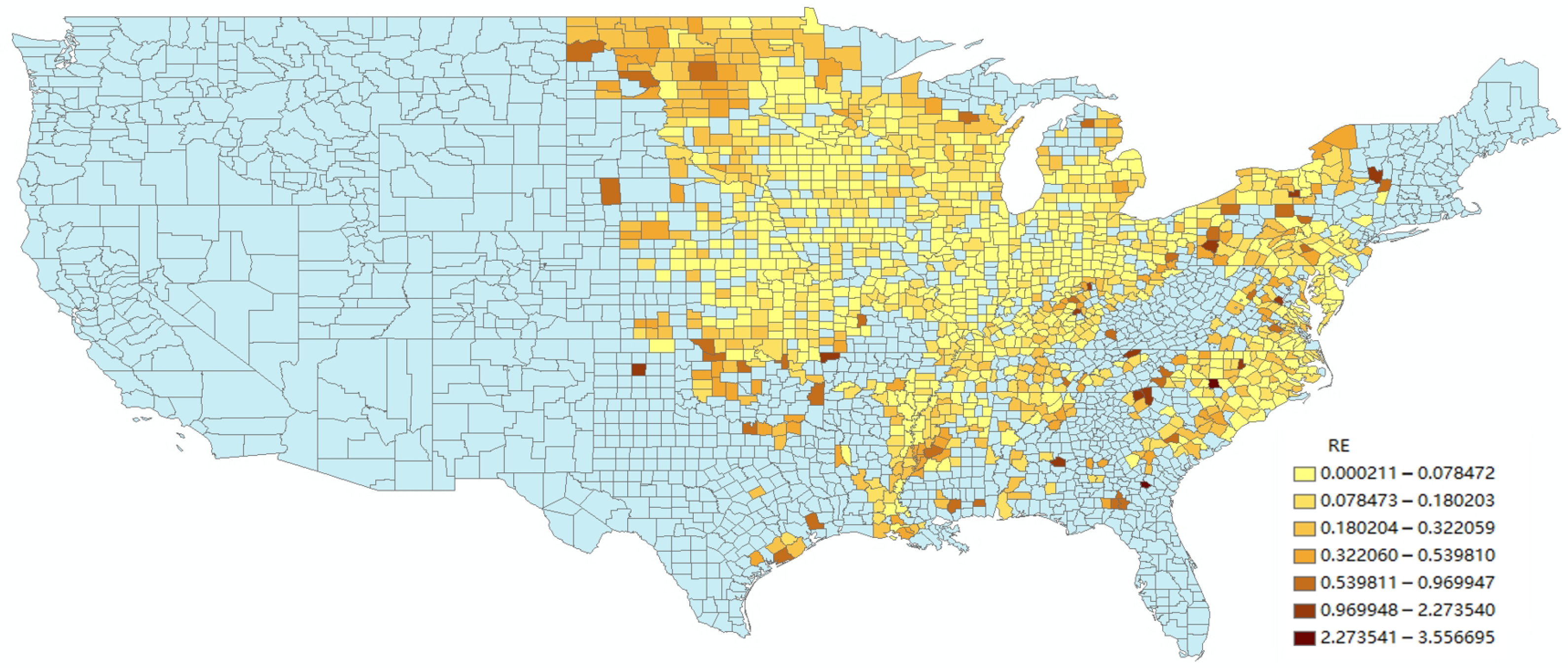
In this section, label distribution smoothing technology (LDST) is proposed to enhance the numerical stability learning ability of the model on imbalanced area data $A$ without changing the true values. When training a network model, accurate area labels are essential for effective training. However, factors such as climate, hydrology, and soil conditions lead to significant variations in crop planting areas across different counties, resulting in unbalanced and long-tailed area data $A$ distributions that complicate the training of planting area estimation models.

From the analysis of the data on soybean planting in the United States in 2020, the data reveal a highly non-uniform distribution, with the value ranging from tens to approximately 10⁵. Therefore, to address the disparity and minimize the influence of significant data variations, a novel function transformation denoted as g(y) is introduced in this study aiming at converting the imbalanced data into a more uniform distribution. This transformation improves the model’s numerical stability and learning ability on imbalanced data while preserving the true values. The function g(y) is defined as (7).

$$\begin{gathered} A^{\prime }=g\left(A\right)=A^{\gamma },\mathrm{s}.\mathrm{t}. \\ \left\{{f_i\cong \left.K\right|f}_i={\sum }_{i=1}^n\mathbb{I}\left(b_j\le a_{n,y}\le b_j+\mathsf{\Delta }\right)\right\} \end{gathered}$$

(7)

where $A=\left\{a_{n,y}\right\}$ and $a_{n,y}$ represent the planting area data of region $n$ in year $y$. And $\mathbb{I}$ is an indicator function. The frequency count in the $i$-th interval of the frequency distribution is denoted as $f_i,\mathrm{a}\mathrm{n}\mathrm{d}K$ represents a constant. The value of γ ranges from 0 to 1, and it is set to 0.4, as determined through pre-experimental analysis.

Based on this transformation, the processed planting area dataset $A^{\prime }$ has mitigated the long-tail effect, with a more balanced distribution pattern ranging from 0 to 250, compared with the original area dataset $A$. After, in the model predicting, it is applied to the original output $\dot{y}$ of the model to obtain the inverse transformation $g^{-1}\left(\dot{y}\right)$ of the final predicted area. This transformation (7) effectively addresses the issue of data imbalance, enhances the model’s interpretability, and enables more robust and insightful crop planting area estimation analyses.

4. Experimental Analysis and Results

This section first introduces the data sources and the dataset construction process. Subsequently, the following five sets of experiments were carried out to validate the accuracy and effectiveness of our proposed planting early area estimation model.

In the accuracy validation experiments, the proposed model was compared with existing advanced techniques (CDL-based and 3D-FPN [22] TMA) to demonstrate that the precision of our approach is among the best in the industry. In practicality validation, predictions were compared with the official forecasts from the USDA to showcase predictive accuracy and effectiveness at both the national and state levels. Additionally, visualizations of the prediction results were utilized to demonstrate their accuracy subjectively. Subsequently, the model’s generalization ability to predict across years was assessed, specifically the capacity to forecast future crop areas without retraining. In the ablation study experiments, the contribution of label smoothing techniques to the convergence of model training and predictive accuracy was examined. In hyper-parameter analysis, the impact of variations in the number of subimages on model predictions was analyzed, highlighting the practical applicability of the method.

4.1. Study Area and Datasets

4.1.1. General Data

The data used in the experiments are CDL data, Crop Area data (county level), Shapefiles of US Administrative regions, and Cropland Mask data. The data range covers the entire United States. As shown in

Table 2. The data used in the end-to-end predictive network.

Data Name	Data Size	Source	Role
CDL	Soybeans	USDA	Input data
Crop Area (county level)	5-3	USDA	Sample label
Shapefiles (county level)	2018	GADM	Units per sample
Cropland Mask	57,500 Acer	GLCLU	Remove useless information

, the CDL is a map of land cover in the United States released by the U.S. Department of Agriculture in January of the following year after planting crops are harvested.

4.1.2. Data Usage

In this study, the training sample is in the county unit.

Table 3. Sample for end-to-end predictive network.

Items	Data Sample	Absolute Error (Acre)
Crop	Soybeans	Type of crop
Region	5-3	The area represented in the sample, (3—Ashley, 5—Arkansas).
Year	2018	The predicted area during training is 2018.
Label	57500 Acer	Training target values for 2018 soybean seeds.
Input Series	2010–2017 CDL	The data used during training. 1855 × 1274 × 8, 18 M.

shows the specific information of the sample of Ashley County, Arkansas, soybean planting area estimation.

In order to increase the richness of the data, in the dataset construction of this paper, the data samples from 2018 to 2020 are used as the training data, 2021 is used as the test data, and 2022 is used as the generalization ability test data. In addition, to verify the different capabilities of the model, the data used in different experiments are shown in

Table 4. Datasets in different experiments for end-to-end predictive network.

Type	Input Series	Label	Accuracy Validation	Practicality Validation	Ablation/Hyper-Parameter Analysis
Training/ Validations	2010–2017 CDL	2018 Area	Ten major producing states	Across America	Illinois
	2011–2018 CDL	2019 Area
	2011–2018 CDL	2020 Area
Testing	2013–2020 CDL	2021 Area
	2014–2021 CDL	2022 Area	------		-------

.

4.2. Metrics

In the early crop planting area estimation experiment, the relative error $RE$ and the absolute error $AE$ are employed as the evaluation metrics to evaluate the accuracy of area estimation. The $AE$ refers to the absolute difference between the predicted area $p\_a$ value and the real area $r\_a$ value, while the $RE$ is the ratio of the $AE$ to the real value. They are both greater than 0, and the computation formula is described as follows. Meanwhile, the lower the error metrics are, the closer the predicted area is to the truth, indicating a better performance of the model.

$$AE=\left|p\_a-r\_a\right|;$$

(8)

$$RE=AE/r\_a$$

(9)

4.3. Results

4.3.1. Model Accuracy Validation

In this part, the proposed model was compared with the mainstream methods to evaluate the differences in predictive accuracy.

As a comparison in model accuracy validation experiments, the CDL-based method adopts USDA CDL data directly as classification data to estimate the planted area, and the 3D-FPN [22,23] method mentioned earlier is the mainstream classical approach method for crop classification. Counting and “Mixed Pixel” [8,13] are selected for the area calculation stage. The counting method directly calculates the number of statistical pixels to determine the area, whereas the “Mixed Pixel” [13] method accounts for area calculation errors associated with different classified crop planting areas. In the experiments, ten main producing states of corn and soybeans were selected for use in 2021. The RE is used in

Table 5. Comparison results of the two-stage method for the main producing states in 2021 (RE).

Types	State Id	State	End-to-End	CDL-Based 1		3D-FPN [22]
				Counting	“Mixed Pixel” [13]	Counting	“Mixed Pixel” [13]
Soybean	5	Arkansas	5.02%	18.77%	3.91%	20.54%	26.56%
	17	Illinois	0.71%	21.86%	4.76%	3.65%	4.54%
	18	Indiana	0.67%	21.83%	1.51%	0.78%	7.78%
	19	Iowa	4.76%	23.15%	8.43%	13.50%	4.77%
	20	Kansas	1.67%	23.88%	1.15%	5.48%	10.02%
	27	Minnesota	3.55%	16.89%	1.69%	3.69%	10.72%
	29	Missouri	0.61%	19.43%	3.73%	13.95%	19.86%
	31	Nebraska	6.89%	23.21%	8.90%	14.91%	6.98%
	39	Ohio	1.08%	21.80%	0.83%	3.52%	10.39%
	46	South Dakota	16.30%	42.42%	69.69%	3.22%	9.99%
Corn	5	Arkansas	17.55%	23.79%	6.54%	58.78%	94.95%
	17	Illinois	0.66%	18.04%	2.69%	15.09%	2.83%
	18	Indiana	1.55%	19.14%	0.12%	13.91%	2.78%
	19	Iowa	3.56%	16.76%	2.92%	11.38%	0.37%
	20	Kansas	6.04%	18.15%	0.40%	21.00%	5.78%
	27	Minnesota	4.36%	14.33%	0.66%	13.16%	6.15%
	29	Missouri	3.03%	25.37%	4.34%	24.92%	9.02%
	31	Nebraska	4.75%	11.04%	2.38%	14.66%	5.69%
	39	Ohio	5.47%	25.41%	5.74%	17.51%	7.43%
	46	South Dakota	7.01%	15.15%	0.10%	10.83%	1.62%
Earliest Acquired Time			March 2021	January 2022		September 2021

¹ Note: CDL is a map of land cover in the United States released by the U.S. Department of Agriculture in January of the following year after planting crops are harvested. The optimal metrics from various methods have been highlighted in bold within the table, with the same converntion maintained for subsequent tables.

and the average error is used in

Table 6. Comparison results of the two-stage method in 2021 (Average Error).

Types	State Id	State	End-to-End	CDL-Based 1	3D-FPN [22]
				“Mixed Pixel” [13]	“Mixed Pixel” [13]
Soybean	5	Arkansas	26.56%	11.67%	35.98%
	17	Illinois	4.54%	6.79%	12.20%
	18	Indiana	7.78%	6.29%	15.77%
	19	Iowa	4.77%	8.37%	7.21%
	20	Kansas	10.02%	9.86%	65.60%
	27	Minnesota	10.72%	8.44%	17.39%
	29	Missouri	19.86%	11.96%	32.16%
	31	Nebraska	6.98%	11.15%	17.79%
	39	Ohio	10.39%	8.09%	18.37%
	46	South Dakota	9.99%	10.38%	13.10%
Corn	5	Arkansas	24.11%	10.21%	100.44%
	17	Illinois	9.76%	4.98%	6.43%
	18	Indiana	6.01%	8.11%	9.81%
	19	Iowa	8.01%	2.99%	4.20%
	20	Kansas	9.54%	5.54%	33.98%
	27	Minnesota	11.14%	4.49%	15.66%
	29	Missouri	14.93%	8.17%	20.32%
	31	Nebraska	7.56%	4.34%	8.42%
	39	Ohio	9.38%	11.21%	9.40%
	46	South Dakota	13.37%	12.87%	9.50%

.

It is evident that there are certain errors in the classification results within the two-stage area estimation methods; consequently, the corrected results are significantly better than those obtained through direct counting. The proposed end-to-end method outperforms the traditional 3D-FPN approach and shows comparable results to the corrected CDL outcomes. This can be attributed to using historical CDL images as input data for the end-to-end method, which also explains the less satisfactory prediction performance observed in South Dakota.

Additionally, to verify the effectiveness of the proposed method compared with the temporal attention-based network, five regions were randomly selected in Illinois in 2021 for validation. The results obtained by the TMA method were directly calculated using the counting method and shown in

Table 7. Comparison results of the two-stage method for five counties in Illinois in 2021 (TMA).

Types	State_County	Standard Area	End-to-End	TMA (Counting)
Soybean	17_117	171,500	1.23%	53.04%
	17_23	98,500	0.97%	58.46%
	17_5	81,700	5.25%	42.03%
	17_105	286,000	3.80%	39.46%
	17_53	135,500	3.69%	59.68%
Average Error			2.99%	50.53%
Corn	17_117	177,000	3.90%	30.93%
	17_23	90,700	0.89%	36.69%
	17_5	72,200	9.77%	13.51%
	17_105	289,000	7.11%	22.34%
	17_53	135,000	5.54%	30.73%
Average Error			5.44%	26.84%

. It can be seen from the table that the error of the proposed method in this paper is one order of magnitude smaller than that of the TMA method, which fully demonstrates the superiority.

Most importantly, the 3D-FPN method and TMA method, which rely on time series remote sensing, can achieve more accurate results after September of the current year, when the corn and soybean crops are booming. In contrast, CDL data for the same year are not released until January of the following year. Therefore, the proposed method can significantly advance the timing of area estimation. Moreover, this method simplifies the area estimation process while still achieving strong performance.

4.3.2. Model Practicality Validation

In this part, predictions were compared with the official forecasts from the USDA to showcase predictive accuracy and effectiveness at both the national and state levels. Additionally, visualizations of the prediction results were utilized to demonstrate their accuracy subjectively.

• Nation Level

This study has selected the authoritative prediction data from the “Monthly Supply and Demand Report” published monthly by the United States Department of Agriculture (USDA) as the benchmark for practicality validation comparison to ensure the accuracy and comparability of the research results. As an official agency of the US government, the USDA is responsible for collecting, analyzing, and releasing predictive data. The prediction data of the USDA is derived through on-site agricultural surveys, the application of statistical models, and comprehensive market analysis. The integrated use of these methods ensures the reliability and practicality of the prediction data.

The experiments conducted on the corn and soybean planting area estimation in 2021 show that the accuracy of our proposed planting area prediction model outperforms the prediction results published by the USDA in terms of RE between the cultivated area and the predicted area. As shown in

Table 8. Nation-level results in 2021.

Types	Methods	Absolute Error (Acre)	Relative Error (RE)
Soybean	End-to-End	3,241,144	3.72%
	USDA	4,000,000	4.70%
Corn	End-to-End	625,639	0.67%
	USDA	2,452,000	2.63%

, the relative error of soybean planting area estimated by our proposed end-to-end predictive network is 3.72%, which is about 1% lower than the USDA predicted data. Similarly, the relative error of corn conducted by the proposed network is 0.67%; however, the relative error of corn predicted by the USDA is 2.63%.

The achievement of our proposed model is attributed to the capability to effectively incorporate information from administrative regions of varying sizes into the network for learning. Moreover, it is crucial to predict current planting areas based on the abundant historical planting datasets. The outperformance experiment results conducted on the national level in the U.S. not only confirm the high efficacy of our multi-subimage technique in addressing the challenge of variable data input sizes in early planting area predictions but also illustrate the feasibility of predicting future planting patterns based on historical planting data. Furthermore, the proposed end-to-end network is capable of avoiding the errors associated with the two-stage area calculation methods and shows high practicality.

• State Level

To research the applicability of our proposed end-to-end predictive network for accurate early crop planting area estimation at the state level, more prediction results at the state level are illustrated in Figure 4. It should be noted that the crop planting area estimation results at the state level have not been included in the supply and demand reports published by the USDA method. Therefore, the errors of planting area estimation results at the state level in this section are computed based on the difference between the prediction result and the real planting area after harvest in the current year.

It can be seen from Figure 4 that the proposed method has good practicality. The prediction accuracy is high not only at the national level but also at the state level for the vast majority of states. Due to the difference in planting patterns between sparse crop areas and common planting patterns, areas with fragmented and sparse planting tend to have greater errors, such as Georgia.

The analysis of crop planting area estimation at the state level reveals that the end-to-end predictive network excels in estimating early planting areas at the main corn and soybean-producing states over non-producing ones. Specifically, the abundance of data in these states enables our model to more accurately detect planting trends and characteristics, thus improving prediction accuracy.

• Visualizing Prediction Results

To show the prediction effect of the model, the relative error of the prediction in 2021 on the soybean dataset is summarized in Figure 5. The figure shows that the relative error is below 7% for most counties in the county-level regions. It meets the needs of most practical applications.

Six regions were randomly selected for the area estimation task of corn and soybean; the prediction ability of the model is visualized in Figure 6. It is an intuitive demonstration of the difficulty of the problem to be solved in this paper, especially between the predicted results, and the label of soybean in Mcleod Minnesota is 227 acres only.

4.3.3. Model Generalization Capability

To research the ability of the end-to-end model to predict across years without retraining, in this section, the trained optimal planting area estimation model is directly utilized to predict the soybean and corn planting area.

Table 9. Nation-level generalization ability results.

Types	Year	Relative Error (RE)
Soybean	2022	1.30%
Corn	2022	6.47%

shows the results of the generalization ability test. The planting area estimation results in 2022 show that the relative errors for the cross-year prediction of the soybean and corn planting areas are 1.3% and 6.47%, respectively.

The results demonstrate the effectiveness of our proposed end-to-end predictive network for accurate early crop planting area estimation. Especially, our proposed planting area estimation method can achieve accurate predictions across a year gap without re-training the prediction model, which presents excellent generalization ability. The outstanding performance is closely related to the long-term historical dataset sequences and the multi-year dataset mixing training strategy used in the training process. It indicates that the model can learn and capture the crop planting patterns across years from the time-series historical planting area dataset, which enables the achievement of higher early predictive results in given years.

4.3.4. Ablation Study

In this part, End-to-End without LDST, End-to-End with LDST, and End-to-End with normalization were designed to validate the contribution of LDST to model training convergence and predictive accuracy.

Table 10. Label smoothing technique validation results for soybean and corn in Illinois.

Types	Methods	Absolute Error (Acre)	Relative Error (RE)
Soybean	End-to-End (-LDST)	Training fails
	End-to-End (LDST)	75,669.25	0.71%
	End-to-End (normalization)	356,710	3.37%
Corn	End-to-End (-LDST)	Training fails
	End-to-End (LDST)	73,038.85	0.66%
	End-to-End (normalization)	608,320	5.53%

illustrates the effectiveness of label smoothing techniques on corn and soybean data from Illinois. The experimental results reveal that when the planting area data are unprocessed, the model struggles to converge due to the wide range of data values and uneven distribution, hindering effective training. In comparison to standard normalization methods, the area relative error (RE) for soybean data decreased by 2.66%, while the area error for corn data dropped to 0.66%.

This analysis indicates that conventional normalization methods merely scale the data to a specified range, which still results in an uneven distribution. In contrast, the proposed label smoothing technique method effectively adjusts the imbalanced area data, creating a more uniform distribution. This adjustment not only reduces the training difficulty for the model but also enhances the accuracy of the predictions.

4.3.5. Hyper-Parameter Analysis

The method proposed has a hyper-parameter that needs to be set, which is the number of subimages for the input model, and it may be difficult to intuitively give a reasonable value. Experiments were conducted based on varying numbers of subimages in the model data, and the results are presented below.

Table 11. Number of subimages validation results for soybean and corn in Illinois (acre).

Types	Methods	Cultivated Area	Predicted Area	RE
Soybean	End-to-End (500)	10,600,000	10,524,330.75	0.71%
	End-to-End (300)	10,600,000	10,287,371.31	2.95%
Corn	End-to-End (500)	11,000,000	10,926,961.15	0.66%
	End-to-End (300)	11,000,000	11,139,742.73	1.27%

presents the area estimation results for corn and soybean data with the number of subimages set to 300 and 500, respectively. The findings indicate that when the number of subimages is set to 500, both experimental groups achieved errors of less than 1%. In contrast, with 300 subimages, the estimation errors increased to 2.95% for corn and 1.27% for soybean. However, these errors remain below 3%, which is acceptable for daily applications. Overall, the experimental results demonstrate that the method is not sensitive to the critical parameter of the number of subimages.

4.3.6. System Optimization for Large-Scale Application Scenarios

To enhance the effectiveness of our methodology in large-scale data applications, we systematically optimized the algorithm execution through four key enhancements. Firstly, we modularized critical components to facilitate code interoperability and eliminate redundant dependencies, enabling flexible implementation. Secondly, we removed non-essential processing steps identified through sensitivity analysis, reducing computational resource consumption by approximately 20%. Thirdly, by restructuring CDL raw data into county-level granular units and converting storage format to int8, we achieved over 70% storage reduction while improving data access efficiency and minimizing training latency. Finally, the implementation of parallelized code execution strategies significantly boosted model processing efficiency.

Compared with previous implementations, these optimizations have yielded remarkable improvements: storage requirements reduced by more than 50%, memory consumption decreased by 30%, and processing throughput increased over threefold. These advancements enable efficient deployment of our end-to-end prediction network for large-scale crop acreage estimation while maintaining comparable accuracy.

4.4. Discussion on Prediction Networks

In this study, the prediction network in the end-to-end prediction network introduces the convolutional network. However, the network structure of this part can be equivalently replaced by other structures. In this part of the research, we verified the VIT model, respectively, in Indiana. The specific results are shown in

Table 12. Comparison of different networks for soybean in Indiana (acres).

Types	Methods	Cultivated Area	Predicted Area	RE
2021	End-to-End (FC)	5,650,000	5,376,210.07	4.8%
	End-to-End (VIT)	5,650,000	5,330,034.75	5.6%
2022	End-to-End (FC)	5,850,000	5,599,580.65	4.3%
	End-to-End (VIT)	5,850,000	5,350,012.12	8.5%

.

The experimental results demonstrate that while multiple algorithmic models exhibit satisfactory predictive performance for the 2021 soybean and corn data forecasting task. This superior performance may be attributed to two key factors: (1) the multi-year Crop Data Layer (CDL) classification dataset presents relatively low learning complexity for cropland area estimation tasks, which can be effectively handled by convolutional neural networks, which is also related to the poor generalization results of the VIT model in 2022; (2) the proposed end-to-end prediction framework features modular architecture that allows flexible network structure adaptation according to specific task requirements.

Notably, the selected CNN architecture demonstrates exceptional computational efficiency and model convergence speed in large-scale cropland area prediction tasks, owing to the streamlined structure and low computational complexity.

5. Conclusions

In this study, an end-to-end predictive network for accurate early crop planting area estimation is proposed, integrating the time-series-based pixel inference method, multi-subimage technology, and label smoothing techniques to address the challenge of early crop planting area estimation. The proposed model not only effectively resolves the area error accumulation issues in the traditional “two-stage” planting area estimation methods but also provides an early planting area estimation before the crops are sown. Furthermore, multi-subimage technology is introduced to tackle the inconsistency in the input sizes of images, and the LDST is employed to mitigate data imbalance in crop planting area estimation.

Our method can obtain the planting area of crops according to the planting trend in the early planting stage, and the accuracy of the model has reached the industry-leading level. At the same time, it has also achieved good results in the practical verification experiment in the United States. However, the error in the area of individual states is slightly larger. Therefore, in future research, it is crucial to develop a high-precision, large-area estimation model that integrates multiple sources of dataset fusion or propose a large model method based on multiple-source datasets to address more challenging problems in agriculture.

References

1. Liu, J.; Wang, L.; Yang, F.; Yang, L.; Wang, X. Remote sensing estimation of crop planting area based on HJ time-series images. Trans. Chin. Soc. Agric. Eng. 2015, 31, 199–206. [Google Scholar]
2. Ben Hassen, T.; El Bilali, H. Impacts of the Russia-Ukraine war on global food security: Towards more sustainable and resilient food systems? Foods 2022, 11, 2301. [Google Scholar] [CrossRef] [PubMed]
3. Yanagi, M. Climate change impacts on wheat production: Reviewing challenges and adaptation strategies. Adv. Resour. Res. 2024, 4, 89–107. [Google Scholar]
4. Aglasan, S.; Roderick; Rejesus, M.; Hagen, S.; Salas, W.; Rejesus, R.M. Cover crops, crop insurance losses, and resilience to extreme weather events. Am. J. Agric. Econ. 2024, 106, 1410–1434. [Google Scholar] [CrossRef]
5. Jiang, W.; Chen, Y. Impact of Russia-Ukraine conflict on the time-frequency and quantile connectedness between energy, metal and agricultural markets. Resour. Policy 2024, 88, 104376. [Google Scholar] [CrossRef]
6. Pandey, D.K.; Mishra, R. Towards sustainable agriculture: Harnessing AI for global food security. Artif. Intell. Agric. 2024, 12, 72–84. [Google Scholar] [CrossRef]
7. Wu, T.T. Analysis on the Influencing Factors of Grain Sown Area in China. Adv. Soc. Sci. 2017, 6, 970–978. [Google Scholar]
8. Chen, K.; Chen, B.; Liu, C.; Li, W.; Zou, Z.; Shi, Z. Rsmamba: Remote sensing image classification with state space model. IEEE Geosci. Remote Sens. Lett. 2024, 21, 8002605. [Google Scholar] [CrossRef]
9. Lv, Z.Y.; Zhang, P.F.; Xie, L.; Benediktsson, J.A.; Lei, T. Iterative sample generation and balance approach for improving hyperspectral remote sensing imagery classification with deep learning network. IEEE Trans. Geosci. Remote Sens. 2024, 62, 5524413. [Google Scholar] [CrossRef]
10. Zheng, Y.; Liu, S.; Chen, H.; Bruzzone, L. Hybrid FusionNet: A hybrid feature fusion framework for multi-source high-resolution remote sensing image classification. IEEE Trans. Geosci. Remote Sens. 2024, 62, 5401714. [Google Scholar] [CrossRef]
11. Bellón, B.; Bégué, A.; Lo Seen, D.; De Almeida, C.A.; Simões, M. A remote sensing approach for regional-scale mapping of agricultural land-use systems based on NDVI time series. Remote Sens. 2017, 9, 600. [Google Scholar] [CrossRef]
12. Zhang, H.; Li, Q.; Wen, N.; Du, X.; Tao, Q.; Tian, Y. Important factors affecting crop acreage estimation based on remote sensing image classification technique. Remote Sens. Land Resour. 2015, 27, 54–61. [Google Scholar]
13. Lu, K.; Ma, Z.; Huo, P.; He, Z.; Zhang, H.; Zheng, X. Mixed Pixel Saturability Based Area Estimation Model on Remote Sensing Image. In Proceedings of the 2023 IEEE 6th International Conference on Pattern Recognition and Artificial Intelligence (PRAI), Haikou, China, 18–20 August 2023; IEEE: New York City, NY, USA, 2023; pp. 751–757. [Google Scholar]
14. Jin, L. Agriculture Area Estimation Based on Classify Error Distribution. Master’s Thesis, Beijing Normal University, Beijing, China, 2012. [Google Scholar]
15. Olofsson, P.; Foody, G.M.; Herold, M.; Stehman, S.V.; Woodcock, C.E.; Wulder, M.A. Good practices for estimating area and assessing accuracy of land change. Remote Sens. Environ. 2014, 148, 42–57. [Google Scholar] [CrossRef]
16. Zhang, H. Research on Crop Landscape Model and Its Effects on Crop Identification and Acreage Estimation. Ph.D. Thesis, The University of Chinese Academy of Sciences, Beijing, China, 2017. [Google Scholar]
17. Zhao, G.; Deng, Z.; Liu, C. Assessment of the Coupling Degree between Agricultural Modernization and the Coordinated Development of Black Soil Protection and Utilization: A Case Study of Heilongjiang Province. Land 2024, 13, 288. [Google Scholar] [CrossRef]
18. Xu, X.; Tang, L.; Kuang, N.; Liu, Y. An image noise reduction and haze removal algorithm based on multi-frame merge. Microelectron. Comput. 2022, 39, 67–74. [Google Scholar]
19. Maxwell, A.E.; Warner, T.A.; Fang, F. Implementation of machine-learning classification in remote sensing: An applied review. Int. J. Remote Sens. 2018, 39, 2784–2817. [Google Scholar] [CrossRef]
20. Tang, B.; Palidan, T.; Bai, J.; Qi, R. Land cover classification method for remote sensing images using CNN and Transformer. Microelectron. Comput. 2024, 41, 64–73. [Google Scholar]
21. Li, C.; Gu, Q.; Cai, Z. Hyperspectral Remote Sensing Image Classification Based on DE and GEP. Microelectron. Comput. 2012, 29, 103–106, 111. [Google Scholar]
22. Gallo, I.; La Grassa, R.; Landro, N.; Boschetti, M. Sentinel 2 time series analysis with 3d feature pyramid network and time domain class activation intervals for crop mapping. ISPRS Int. J. Geo-Inf. 2021, 10, 483. [Google Scholar] [CrossRef]
23. Gallo, I.; Ranghetti, L.; Landro, N.; La Grassa, R.; Boschetti, M. In-season and dynamic crop mapping using 3D convolution neural networks and sentinel-2 time series. ISPRS J. Photogramm. Remote Sens. 2023, 195, 335–352. [Google Scholar] [CrossRef]
24. Yan, S.; Yao, X.; Zhu, D.; Liu, D.; Zhang, L.; Yu, G.; Gao, B.; Yang, J.; Yun, W. Large-scale crop mapping from multi-source optical satellite imageries using machine learning with discrete grids. Int. J. Appl. Earth Obs. Geoinf. 2021, 103, 102485. [Google Scholar] [CrossRef]
25. Yang, L.; Wang, L.; Abubakar, G.A.; Huang, J. High-resolution rice mapping based on SNIC segmentation and multi-source remote sensing images. Remote Sens. 2021, 13, 1148. [Google Scholar] [CrossRef]
26. Wang, H.; Wang, W.; Liu, J. Temporal Memory Attention for Video Semantic Segmentation. In Proceedings of the 2021 IEEE International Conference on Image Processing (ICIP), Anchorage, AK, USA, 19–22 September 2021; pp. 2254–2258. [Google Scholar]
27. Liang, R. Research on Object-Oriented Remote Sensing Image Segmentation and Cornfield Area Estimation Methods. Master’s Thesis, North University of China, Taiyuan, China, 2016. [Google Scholar]
28. Krawczyk, B. Learning from imbalanced data: Open challenges and future directions. Prog. Artif. Intell. 2016, 5, 221–232. [Google Scholar] [CrossRef]
29. Sermanet, P. Overfeat: Integrated Recognition, Localization and Detection Using Convolutional networks. arXiv 2013, arXiv:1312.6229. [Google Scholar]
30. He, K.; Zhang, X.; Ren, S.; Sun, J. Spatial pyramid pooling in deep convolutional networks for visual recognition. IEEE Trans. Pattern Anal. Mach. Intell. 2015, 37, 1904–1916. [Google Scholar] [CrossRef]
31. Long, J.; Shelhamer, E.; Darrell, T. Fully convolutional networks for semantic segmentation. In Proceedings of the IEEE Conference on Computer Vision and Pattern Recognition, Boston, MA, USA, 7–12 June 2015; pp. 3431–3440. [Google Scholar]
32. Mao, H.; Liu, X.; Duffield, N.; Yuan, H.; Ji, S.; Mohanty, B.P. Context-aware deep representation learning for geo-spatiotemporal analysis. In Proceedings of the 2020 IEEE International Conference on Data Mining (ICDM), Sorrento, Italy, 17–20 November 2020; IEEE: New York City, NY, USA, 2020; pp. 392–401. [Google Scholar]
33. You, J.; Li, X.; Low, M.; Lobell, D.; Ermon, S. Deep gaussian process for crop yield prediction based on remote sensing data. In Proceedings of the AAAI Conference on Artificial Intelligence, San Francisco, CA, USA, 4–9 February 2017; Volume 31. [Google Scholar] [CrossRef]
34. Ahmed, T.; Kumar, A.; Casado, C.Á.; Zhang, A.; Hänninen, T.; Loven, L.; López, M.B.; Tarkoma, S. Exponentially Weighted Instance-Aware Repeat Factor Sampling for Long-Tailed Object Detection Model Training in Unmanned Aerial Vehicles Surveillance Scenarios. arXiv 2025, arXiv:2503.21893. [Google Scholar]
35. Lu, K.; Ma, Z.; He, Z.; Huo, P.; Zhang, H. End-to-End Network for Early Crop Planting Area Prediction. In Proceedings of the 2024 7th International Conference on Pattern Recognition and Artificial Intelligence (PRAI), Hangzhou, China, 15–17 August 2024; IEEE: New York City, NY, USA, 2024; pp. 1063–1068. [Google Scholar]
36. He, K.; Zhang, X.; Ren, S.; Sun, J. Delving deep into rectifiers: Surpassing human-level performance on imagenet classification. In Proceedings of the IEEE International Conference on Computer Vision, Santiago, Chile, 7–13 December 2015; pp. 1026–1034. [Google Scholar]
37. Han, W.; Yang, Z.; Di, L.; Mueller, R. CropScape: A Web service based application for exploring and disseminating US conterminous geospatial cropland data products for decision support. Comput. Electron. Agric. 2012, 84, 111–123. [Google Scholar] [CrossRef]
38. Zhang, C.; Di, L.; Yang, Z.; Lin, L.; Yu, E.G.; Yu, Z. Cloud environment for disseminating NASS cropland data layer. In Proceedings of the 2019 8th International Conference on Agro-Geoinformatics (Agro-Geoinformatics), Istanbul, Turkey, 16–19 July 2019; IEEE: New York City, NY, USA, 2019; pp. 1–5. [Google Scholar]
39. USDA-NASS. Cropland Data Layer Metadata. 2022b. Available online: https://www.nass.usda.gov/Research_and_Science/Cropland/Release/ (accessed on 1 January 2009).
Figure 1. Comparison between Brown County and Door County.
Mathematics 13 01656 g001
Figure 2. Overall framework diagram for end-to-end predictive network.
Mathematics 13 01656 g002
Figure 3. Example of processing flow using multi-subimage technology.
Mathematics 13 01656 g003
Figure 4. Comparative analysis of prediction results for soybean and corn. The upper panel illustrates the predicted results for soybean cultivation, presenting the predictions for the cultivated areas in various states in 2021, and the AE is plotted as an orange bar, while the RE is depicted as a blue bar chart. Similarly, the lower panel describes the predictions for corn.
Mathematics 13 01656 g004
Figure 5. RE of 2021 soybean planting area in the United States (part) compared with the data published by USDA. The RE increases as the color gets darker from yellow to brown, shown in the legend at the bottom right. The blue area is the area with missing data at the county level. There are two reasons for the missing: one is the lack of planting situation, and the other is the combination of statistics with neighboring counties in the statistical process. These two cases are not distinguished.
Mathematics 13 01656 g005
Figure 6. Prediction results of soybean and corn planting area at county level (unit: acre).
Mathematics 13 01656 g006