A Modified Phase-Locked Loop with Parameter Self-Tuning Used in the Sensorless Control of Permanent Magnet Synchronous Motors (PMSMs)

Abstract

This paper proposes a sensorless field-oriented control (FOC) strategy for permanent magnet synchronous motors (PMSMs), focusing on rotor flux position estimation based on back-electromotive force (back-EMF) signals. The limitations of conventional phase-locked loop (PLL) techniques for rotor flux position estimation along the motor shaft are analyzed, and an enhanced PLL structure is developed to address these deficiencies.In electric vehicle traction applications, precise flux position estimation alone is insufficient; accurate generation of d–q-axis current commands is equally critical. To address this need, a zero-pole-free PI regulator is designed within the PLL module, enabling more accurate flux estimation. Additionally, a gradient-based self-tuning algorithm is employed to identify system parameters, particularly the stator inductance, enabling the controller to optimize current command generation.Comprehensive system-level simulations have been conducted to validate the effectiveness of the proposed sensorless control scheme. Comparative studies demonstrate that the proposed method significantly improves feasibility and robustness for practical PMSM drive applications.

1. Introduction

Recent advancements in microcontroller technologies have significantly enhanced computational performance while simultaneously reducing system costs, primarily driven by the widespread adoption of high-speed digital signal processing (DSP). These improvements have enabled the implementation of software-based motor control algorithms, reducing the reliance on dedicated hardware components. As a result, the transition from brushed DC motors to AC drives, such as induction motors and permanent magnet synchronous motors (PMSMs), has been accelerated in numerous industrial and consumer applications.

One of the most active research areas in AC motor drives is sensorless field-oriented control (FOC), which eliminates the need for physical sensors to measure rotor speed and position. Instead, rotor position is estimated in real time based solely on voltage and current measurements obtained at the motor terminals.

Rotor position can be estimated at any time by measuring only the stator voltages and currents of the motor. The fundamental structure of sensorless FOC for permanent magnet synchronous motors (PMSMs) was introduced by S. Bolognani et al. in [1].

A comprehensive classification of most estimation schemes for PMSM field-oriented control (FOC) was presented by Lee et al. in [2].

Y. Park et al. [3] classified ${\theta }_{rf}-{\stackrel{⌢}{\theta }}_{rf}$ estimator algorithms into two categories, each specifically designed for operation in either high-speed or low-speed regions.

Conventional estimation techniques become ineffective in the low-speed region, where the back-electromotive force (back-EMF) of the motor is inherently weak and unreliable. To address this issue, high-frequency signals are injected along the d-axis of the rotating reference frame aligned with the rotor flux. The resulting q-axis response contains information that can be utilized to estimate the rotor flux axis angle error, denoted as $\widehat{\epsilon }$. This approach, commonly referred to as high-frequency signal injection, has been extensively investigated in the literature [4,5,6].

On the other hand, when the rotor speed is sufficiently high such that the back-electromotive force (back-EMF) can be reliably observed, it can be utilized to estimate ${\theta }_{rf}-{\stackrel{⌢}{\theta }}_{rf}$ [7,8,9,10,11,12]. Christian [13] provided a rigorous mathematical analysis of the closed-loop system formed by the combination of a PMSM extended state observer and a PI controller.

Based on empirical rules, the threshold for distinguishing low-speed operation is typically set at approximately 5% of the motor’s rated speed. As noted by Bolognani et al. [1], although the algorithms for ${\theta }_{rf}-{\stackrel{⌢}{\theta }}_{rf}$ estimation differ between low-speed and high-speed regions, the underlying operational sequence of speed and position estimators follows the same structure as a phase-locked loop (PLL).

In addition, Guozhong et al. [14] identified that the structure proposed by Bolognani et al. [1] encounters issues during reverse operation. To address this problem, they modified the PLL structure by squaring the sine and cosine signals and processing them at twice the fundamental frequency. This modification effectively resolves the reverse operation issue. Furthermore, the authors introduced an I/F startup control strategy to overcome the limitations of back-EMF-based algorithms in the low-speed region.

Oleg V. Nos [15] proposed a method for estimating back-electromotive force (back-EMF) using a sliding mode observer, which relies on the error between the actual and estimated stator currents. The estimated back-EMF is then processed through a complex coordinate filter (CCF) and a phase angle controller (PAC), with adjustments made based on the difference between the estimated and actual angular velocities. This framework forms the basis of the novel PLL structure proposed by the author. However, it should be noted that the PAC remains based on the conventional PI regulator.

Wu et al. [16] pointed out that conventional phase-locked loop (PLL) structures fail under reverse rotational conditions, leading to positive feedback and eventual loss of control. To address this issue, a generalized PLL (GPLL) architecture was proposed, which combines two PLL structures operating in both the α-β and d-q reference frames. By mutually calibrating the estimated outputs from each frame, the GPLL effectively resolves issues related to reverse rotation and low-speed operation. However, it still relies on the conventional proportional–integral (PI) regulator.

Zdenek [17] pointed out that a fixed bandwidth in phase-locked loop (PLL) structures is insufficient to accommodate the wide speed range requirements of motor applications. To address this limitation, a self-tuning mechanism based on the gradient method was incorporated into the PI regulator within the PLL, allowing the proportional and integral gains to be optimized in real time based on the estimated states and errors.

Because there are many limitations in a phase-locked loop, the above structure may not be realizable. The performance of a PLL may not be satisfactory even if it can be used. The problems induced by a general PLL will be presented, and the modified strategy will be provided in this paper. In addition, a simulation is performed to verify the feasibility of the proposed strategy.

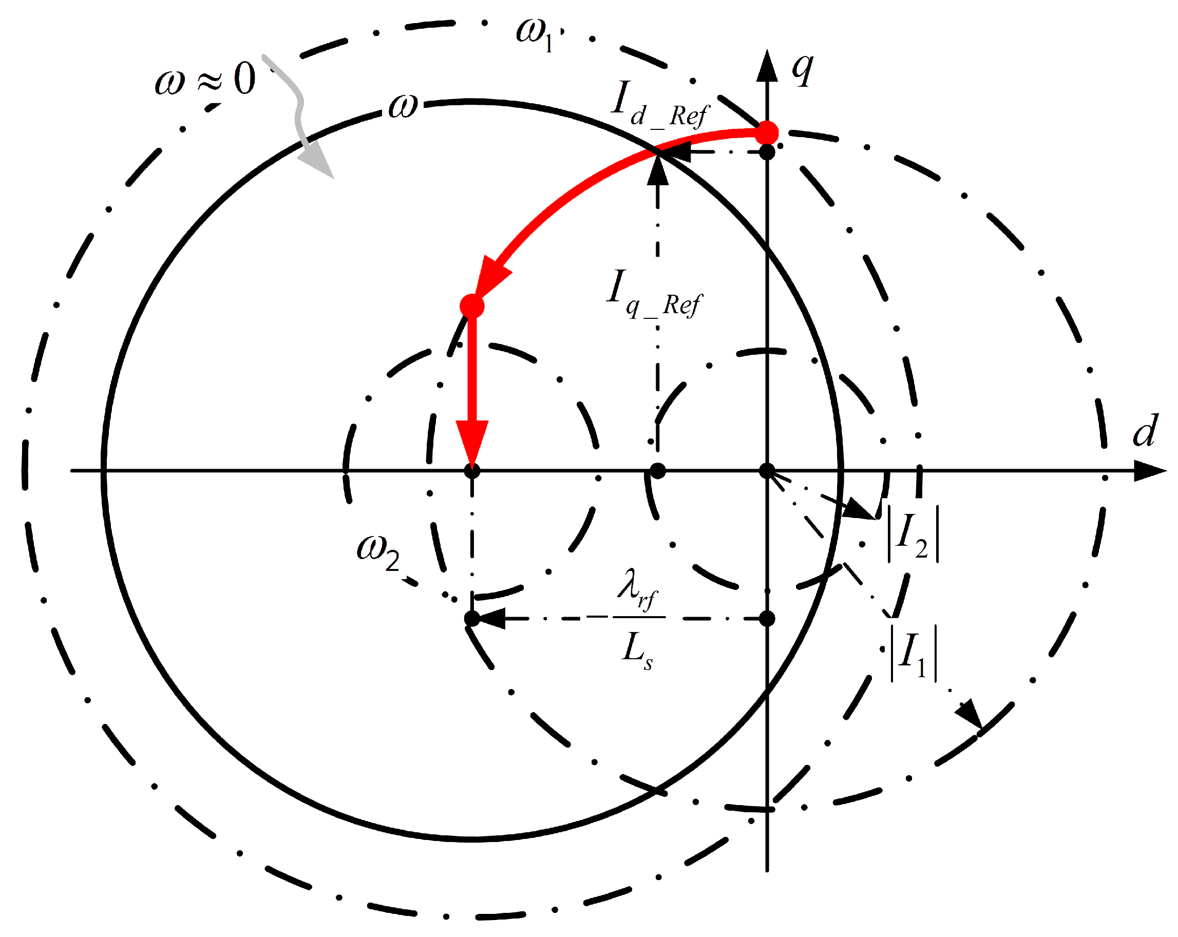
In the operation of field-oriented control (FOC), it is essential not only to accurately lock onto the rotor flux position but also to optimally determine the placement of the stator current vector. This requirement becomes particularly critical in electric vehicle applications, where both the battery voltage and motor output power are limited. The accelerator pedal reflects the driver’s torque demand, and the controller must subsequently determine the appropriate magnitude of the current commands. Before doing so, it is necessary to consider constraints such as the battery voltage and vehicle speed. Interestingly, in high-speed regions, the required torque tends to be inversely proportional to the vehicle speed. As a result, field weakening control becomes an effective means to optimize the power-to-size ratio of the drive unit.

Bimal [18] proposed a formulation for surface-mounted permanent magnet synchronous motors (SPMSMs), as illustrated in Figure 1, satisfying the following:

$${\left(i_d-C\right)}^2+i_q^2={\displaystyle \frac{L_s^2}{{\omega }^2{V}_{DC}^2}},i_d^2+i_q^2={\left|I_x\right|}^2$$

(1)

where $C=-{\displaystyle \raisebox{1ex}{${\lambda }_{rf}$}\!\left/ \!\raisebox{-1ex}{$L_s$}\right.}$ and $\left|I_x\right|$ represent the radii of current command circles, $V_{DC}$ is the DC bus voltage, $\omega$ is the electrical angular velocity, $L_s$ is the stator inductance, and ${\lambda }_{rf}$ is the rotor flux linkage. Based on this relationship, it can be derived that once $\omega$ rises to ${\omega }_1={\displaystyle \frac{V_{DC}}{\sqrt{L_s^2{I}_x^2+{\lambda }_{rf}^2}}}$, the system must enter the field-weakening region where $i_{d\_Ref}$ and $i_{q\_Ref}$ vary with speed, while still satisfying the current circle conditions defined by $i_{d\_Ref}={\displaystyle \frac{1}{2L_s{\lambda }_{rf}}}\left({\displaystyle \frac{V_{DC}^2}{{\omega }^2}}-{\lambda }_{rf}^2-L_s^2{I}_x^2\right)$ and $i_{q\_Ref}=\sqrt{I_x^2-i_{d\_Ref}^2}$. The red curve shown in Figure 1 depicts the trajectory of the current command as a function of rotor speed. Furthermore, in scenarios involving vehicle coasting, regenerative braking, and battery range extension, the planning of the current command trajectory becomes critically dependent on the accurate identification of system parameters. Therefore, the objective of this work is to dynamically adapt system parameters in response to varying operating conditions, while simultaneously maintaining precise rotor flux position estimation.

The remainder of this paper is organized as follows. Section 2 derives the importance and theoretical foundation of back-electromotive force (back-EMF) estimation for sensorless operation based on motor equations. Section 3 reviews the fundamental theory of phase-locked loops (PLLs) from the perspective of communication systems, where PLLs were first utilized, and proposes modifications to enhance stability. Section 4 establishes a comprehensive simulation framework, incorporating both the conventional back-EMF estimation method (integrated with PLL) and the improved structure proposed by Shuo [19], under a predefined power-down restart scenario. Section 5 presents a gradient search method for dynamically tracking the actual stator inductance. Section 6 applies the proposed concepts under identical conditions for further comparative simulations. Finally, Section 7 discusses and evaluates the advantages and limitations of the three investigated architectures.

2. Mathematical Model of PMSM Used for Estimating the Back-EMF

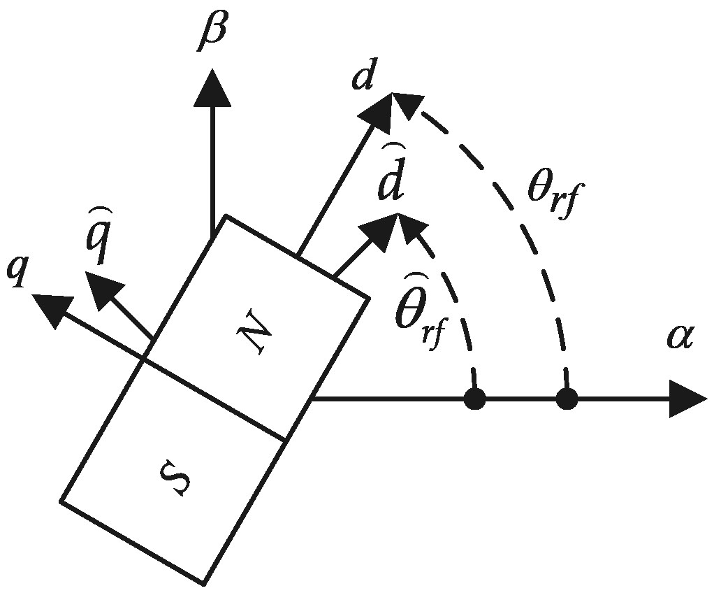
There are two conventional coordinate systems used in the FOC of a motor: the rotating $d-q$ coordinate system, where the $d$-axis aligns with the N pole, and the stationary $\alpha -\beta$ coordinate system, where the $\alpha$ axis aligns with the $a$ phase winding coil of the stator. The relationship between them is shown in Figure 2. Furthermore, there is still another coordinate system, $\stackrel{⌢}{d}-\stackrel{⌢}{q}$, due to the inaccurate estimation.

In PMSMs, the mathematical model of the interior permanentmagnet synchronousmotor (IPMSM) is the most complex. Lee et al. [2] derived its governing equation in the $\alpha -\beta$ reference frame as follows:

$$\left[\begin{array}{c}{v}_{\alpha }\\ v_{\beta }\end{array}\right]=\left[\begin{array}{cc}R+\left(\begin{array}{l}{L}_0+\\ L_1\cos 2{\theta }_{rf}\end{array}\right)D& \left(L_1\sin 2{\theta }_{rf}\right)D\\ \left(L_1\sin 2{\theta }_{rf}\right)D& R+\left(\begin{array}{l}{L}_0-\\ L_1\cos 2{\theta }_{rf}\end{array}\right)D\end{array}\right]\cdot \left[\begin{array}{c}{i}_{\alpha }\\ i_{\beta }\end{array}\right]+{\omega }_{rf}{\lambda }_{PM}\left[\begin{array}{c}-\sin {\theta }_{rf}\\ \cos {\theta }_{rf}\end{array}\right]$$

(2)

where:

• $\begin{array}{cc}{v}_{\alpha },& v_{\beta }\end{array}$: stator voltages in the $\alpha -\beta$ frame.
• $\begin{array}{cc}{i}_{\alpha },& i_{\beta }\end{array}$: stator currents in the $\alpha -\beta$ frame.
• $R$: stator resistance.
• $D$: differential operator.
• ${\lambda }_{PM}$: permanent magnet flux linkage.
• ${\theta }_{rf}$: rotor angular position.
• ${\omega }_{rf}$: rotor angular velocity.

$\begin{array}{cc}{L}_0={\displaystyle \frac{L_d+L_q}{2}},& L_1={\displaystyle \frac{L_d-L_q}{2}}\end{array}$, $L_d$, and $L_q$ are the $d-$ and $q-$axis inductances.

As for the surface-mountedpermanentmagnet synchronousmotor (SPMSM), (2) can be simplified because $L_d=L_q=L_s$ in this type, as follows:

$$\left[\begin{array}{c}{v}_{\alpha }\\ v_{\beta }\end{array}\right]=\left[\begin{array}{cc}R+L_{s}D& 0\\ 0& R+L_{s}D\end{array}\right]\left[\begin{array}{c}{i}_{\alpha }\\ i_{\beta }\end{array}\right]+\left[\begin{array}{c}{e}_{\alpha }\\ e_{\beta }\end{array}\right]$$

(3)

where $\left[\begin{array}{c}{e}_{\alpha }\\ e_{\beta }\end{array}\right]={\omega }_{rf}{\lambda }_{PM}\left[\begin{array}{c}-\sin {\theta }_{rf}\\ \cos {\theta }_{rf}\end{array}\right]$, which are indeed the back-EMF.

The mathematical model of an IPMSM in the $d-q$ reference frame can be described as follows:

$$\left[\begin{array}{c}{v}_d\\ v_q\end{array}\right]=\left[\begin{array}{cc}R+L_{d}D& -{\omega }_{rf}{L}_q\\ {\omega }_{rf}{L}_d& R+L_{q}D\end{array}\right]\left[\begin{array}{c}{i}_d\\ i_q\end{array}\right]+\left[\begin{array}{c}0\\ {\omega }_{rf}{\lambda }_{PM}\end{array}\right]$$

(4)

Equation (4) can be reduced to (5) if SPMSM is presented in the above reference frame:

$$\left[\begin{array}{c}{v}_d\\ v_q\end{array}\right]=\left[\begin{array}{cc}R+L_{s}D& -{\omega }_{rf}{L}_s\\ {\omega }_{rf}{L}_s& R+L_{s}D\end{array}\right]\left[\begin{array}{c}{i}_d\\ i_q\end{array}\right]+\left[\begin{array}{c}0\\ {\omega }_{rf}{\lambda }_{PM}\end{array}\right]$$

(5)

Equation (5) can be split into two scalar equations:

$$\begin{array}{cc}\left(R+L_{s}D\right) i_d=v_d^{\prime }+{\omega }_{rf}{L}_s{i}_q,& \left(R+L_{s}D\right) i_q=v_q^{\prime }-{\omega }_{rf}{L}_s{i}_d-{\omega }_{rf}{\lambda }_{PM}\end{array}$$

(6)

Hence, we constrain the scope of this paper in SPMSM and build the basic FOC according to the proposition by Lee et al. [2]. The decoupling compensation scheme presented in this paper is shown in Figure 3.

In this scheme, if the $v_q^{\prime }$ and $v_d^{\prime }$ in (6) are replaced by $v_q^{*}=v_q^{\prime }+{\stackrel{⌢}{\omega }}_{rf}{L}_s{i}_d+{\stackrel{⌢}{\omega }}_{rf}{\lambda }_{PM}$ and $v_d^{*}=v_d^{\prime }-{\stackrel{⌢}{\omega }}_{rf}{L}_s{i}_q$, thefollowing is implied:

$$\begin{array}{cc}\left(R+L_{s}D\right)i_d=v_d^{\prime },& \left(R+L_{s}D\right)i_q=v_q^{\prime }\end{array}$$

(7)

These two equations are linear and independent of each other. This is the aim of this scheme. In Figure 3, 5% of the rating speed is used as the level of switching between two modes. A high-frequency signal (e.g., $a=5$ and ${\omega }_{hf}=100k$) will be added to the command voltage on the $d$-axis when the rotor speed is lower than this level. Otherwise, the back-EMF method will be used and developed when the speed exceeds the level.

By rewriting (3), one can obtain the following:

$$\begin{array}{cc}{v}_{\alpha }^{*}-e_{\alpha }=\left(R+L_{s}D\right) i_{\alpha },& e_{\alpha }=-{\omega }_{rf}{\lambda }_{PM}\sin {\theta }_{rf}\\ v_{\beta }^{*}-e_{\beta }=\left(R+L_{s}D\right) i_{\beta },& e_{\beta }={\omega }_{rf}{\lambda }_{PM}\cos {\theta }_{rf}\end{array}.$$

(8)

Equation (8) is schematically represented in Figure 4.

It is important to emphasize that although the back-electromotive force (back-EMF) components $e_{\alpha }$ and $e_{\beta }$ represent actual physical quantities, they can be easily measured only when the machine operates in generator mode, with mechanical energy input at the shaft. In practical motor operation, the terminal back-EMF is overwhelmed by the pulse-width modulated (PWM) square-wave voltage applied to the stator, rendering direct measurement infeasible. Consequently, observer-based methods must be employed to estimate the back-EMF in real time.

Because ${\overrightarrow{v}}^{*}=\left[\begin{array}{c}{v}_{\alpha }^{*}\\ v_{\beta }^{*}\end{array}\right]$, $\overrightarrow{i}=\left[\begin{array}{c}{i}_{\alpha }\\ i_{\beta }\end{array}\right]$, and ${\stackrel{⌢}{\theta }}_{rf}$ denote the command voltage, the feedback current and the estimated angle, respectively, and are known. Although (3) is the governing equation, we can rebuild the behavior of the system by numeric algorithms if the system parameters ${\stackrel{⌢}{R}}_s$ and ${\stackrel{⌢}{L}}_s$ are also known. Therefore,${\stackrel{⌢}{X}}_{\alpha }$ and ${\stackrel{⌢}{X}}_{\beta }$ will approach the back-EMF $e_{\alpha }$ and $e_{\beta }$ of the system when the current errors $\Delta i_{\alpha }$ and $\Delta i_{\beta }$ converge to the minimum values, that is, if the correct value for estimating back-EMF can be obtained, we can obtain the following:

$$\left[\begin{array}{c}{\stackrel{⌢}{X}}_{\alpha }\\ {\stackrel{⌢}{X}}_{\beta }\end{array}\right]=A•\left[\begin{array}{c}-\sin {\theta }_{rf}\\ \cos {\theta }_{rf}\end{array}\right],$$

(9)

where $A$ is a positive value. According to Kim et al. [20], although ${\stackrel{⌢}{\theta }}_{rf}$ can be derived from

$${\stackrel{⌢}{\theta }}_{rf}=-{\tan }^{-1}{\displaystyle \frac{{\stackrel{⌢}{X}}_{\alpha }}{{\stackrel{⌢}{X}}_{\beta }}},$$

(10)

the ${\tan }^{-1}\left(•\right)$ is not a well-defined function because the positions satisfied with ${\stackrel{⌢}{\theta }}_{rf}={\displaystyle \frac{2n+1}{2}}\pi$ are all singular points. So, this approach cannot solve this problem completely. Moreover, the calculation of ${\tan }^{-1}\left(•\right)$ is difficult to execute on a fixed point and low-cost processor. In summary, we will propose an approach that evaluates the estimated error of the angular position to produce a valid ${\stackrel{⌢}{\theta }}_{rf}$.

3. The Modified Phase-Locked Loop

In the last process, as shownin Figure 4, the estimated back-EMF (${\stackrel{⌢}{X}}_{\alpha }$ and ${\stackrel{⌢}{X}}_{\beta }$) in (8) is modulated with $\cos {\stackrel{⌢}{\theta }}_{rf}$ and $\sin {\stackrel{⌢}{\theta }}_{rf}$ into the following:

$$-{\stackrel{⌢}{X}}_{\alpha }\cos {\stackrel{⌢}{\theta }}_{rf}-{\stackrel{⌢}{X}}_{\beta }\sin {\stackrel{⌢}{\theta }}_{rf}=A\sin {\theta }_{rf}\cdot \cos {\stackrel{⌢}{\theta }}_{rf}-A\cos {\theta }_{rf}\cdot \sin {\stackrel{⌢}{\theta }}_{rf}=A\sin \left({\theta }_{rf}-{\widehat{\theta }}_{rf}\right)\equiv \stackrel{⌢}{\epsilon }.$$

(11)

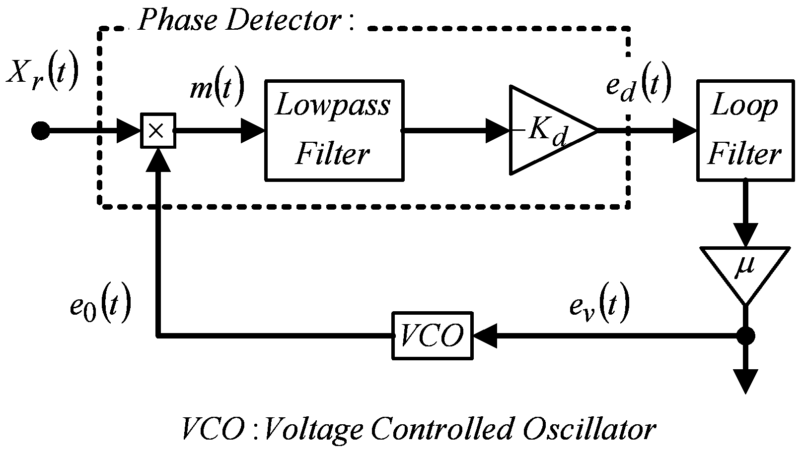
Lee introduced a common communication field technique (i.e.,phase-lockedloop) in this process [4]. The conventional definition of a PLL in this field is shown in Figure 5. Jun Cai [21] summarized the evolution of phase-locked loop (PLL) structures, highlighting the challenges encountered at each stage and the corresponding improvement strategies developed over time. The progression began with conventional PLLs, evolved into modified versions, incorporated built-in filters, and ultimately led to the development of modern PLL architectures. At each stage, enhancements were achieved but often at the cost of certain performance trade-offs.

The signals presented in Figure 5 are described as follows:

$$\begin{array}{c}{X}_r\left(t\right)=A_c\cos \left[{\omega }_{c}t+\theta \left(t\right)\right], e_0\left(t\right)=A_v\sin \left[{\omega }_{c}t+\stackrel{⌢}{\theta }\left(t\right)\right],\\ \Rightarrow m\left(t\right)=A_c{A}_v\cos \left[{\omega }_{c}t+\theta \left(t\right)\right]\sin \left[{\omega }_{c}t+\stackrel{⌢}{\theta }\left(t\right)\right]\\ ={\displaystyle \frac{1}{2}}{A}_c{A}_v\left\{\sin \left[2{\omega }_{c}t+\theta \left(t\right)+\stackrel{⌢}{\theta }\left(t\right)\right]-\sin \left[\theta \left(t\right)-\stackrel{⌢}{\theta }\left(t\right)\right]\right\}\\ \Rightarrow e_d\left(t\right)={\displaystyle \frac{A_c{A}_v{K}_d}{2}}\sin \left[\theta \left(t\right)-\stackrel{⌢}{\theta }\left(t\right)\right], {\displaystyle \frac{d\stackrel{⌢}{\theta }\left(t\right)}{dt}}=K_v{e}_v\left(t\right)\end{array}$$

(12)

As shown in Figure 5, the signal definitions correspond to (12). Figure 5 can be equivalently represented by Figure 6. After simplification, it is observed that $X_r\left(t\right)$ must exhibit stable oscillatory behavior, while the phase component $\theta \left(t\right)$ should vary slowly. Moreover, near-linear system behavior, as illustrated by $\theta \left(t\right)\approx \stackrel{⌢}{\theta }\left(t\right)$, occurs only when the phase is nearly locked. Otherwise, the analysis must consider the nonlinear characteristics depicted in the upper portion of Figure 6. To illustrate the invalidity of $\sin \left[\varphi \left(t\right)\right]\approx \varphi \left(t\right)$, the case where the loop filter exhibits a unity gain (i.e., a special case of $G_{loop}\left(s\right)=1$) is first considered. Based on Figure 6, $\stackrel{⌢}{\theta }\left(t\right)=K_t{\displaystyle {\int }_0^t\sin \left[\theta \left(t\right)-\stackrel{⌢}{\theta }\left(t\right)\right]dt}$ can be derived, resulting in the following:

$$K_t={\displaystyle \frac{1}{2}}{A}_c{A}_v{K}_d{K}_v\Rightarrow {\displaystyle \frac{d\stackrel{⌢}{\theta }\left(t\right)}{dt}}=K_t\sin \left[\theta \left(t\right)-\stackrel{⌢}{\theta }\left(t\right)\right]$$

(13)

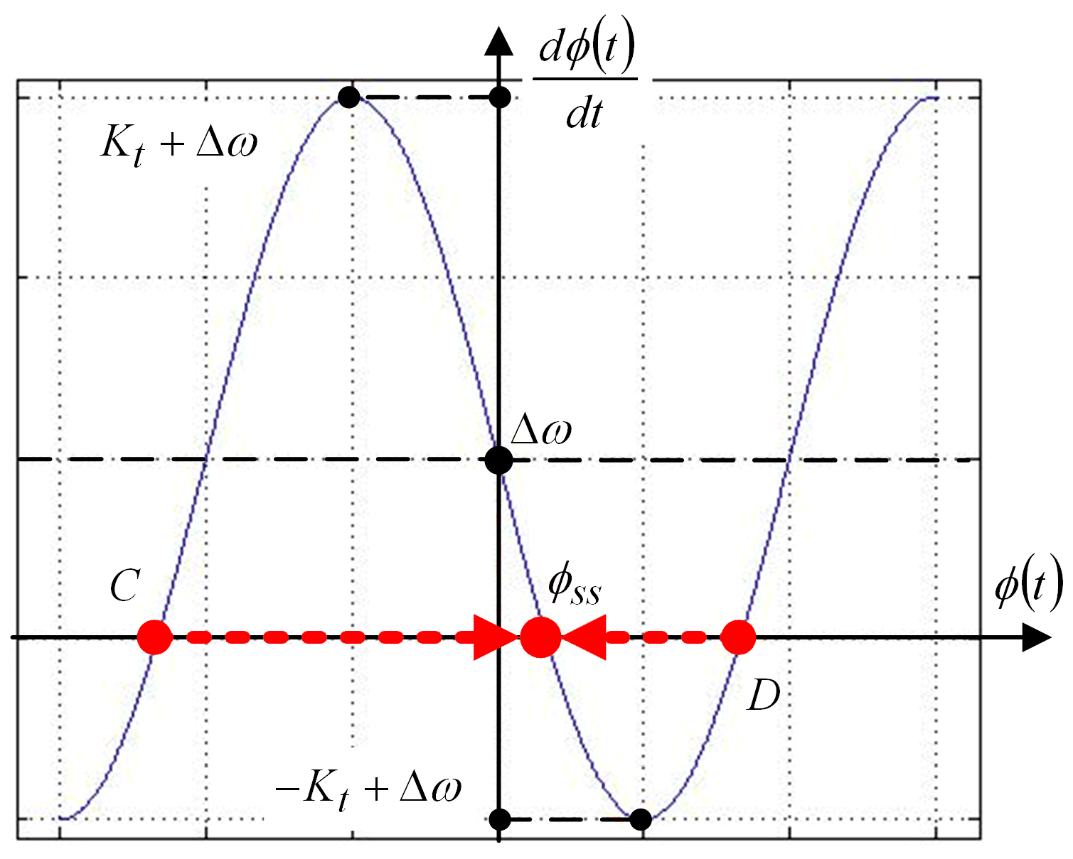
If ${\displaystyle \frac{d\theta }{dt}}=\Delta \omega$ denotes the frequency drift of the original input signal,

$$\Rightarrow {\displaystyle \frac{d\varphi \left(t\right)}{dt}}=-K_t\sin \varphi \left(t\right)+\Delta \omega$$

(14)

holds. According to (14), the corresponding phase trajectory is depicted in Figure 7.

From Figure 7, the error between the actual angle $\theta \left(t\right)$ and the tracking angle $\stackrel{⌢}{\theta }\left(t\right)$ will converge to ${\varphi }_{ss}$ from the right to the left if the initial value (i.e., ${\varphi }_0={\theta }_0-{\stackrel{⌢}{\theta }}_0$) falls to the region between points $D$ and ${\varphi }_{ss}$, where ${\varphi }_{ss}={\sin }^{-1}{\displaystyle \frac{\Delta \omega }{K_t}}$. On the contrary, this error will converge to ${\varphi }_{ss}$ from the left to the right if the initial value falls to the region between points $C$ and ${\varphi }_{ss}$. Therefore, it will converge to ${\varphi }_{ss}+2\pi$ ($\stackrel{⌢}{\theta }$ behind $\theta$ one circle) if ${\varphi }_0$ falls to the right side of point $D$ and ${\phi }_{ss}-2\pi$ ($\stackrel{⌢}{\theta }$ ahead $\theta$ one circle) if ${\varphi }_0$ falls to the left side of point $C$. The ${\varphi }_{ss}$ decreases when $K_t$ increases. In summary, ${\varphi }_{ss}$ is the steady-state error when the phase portrayed intersects with the horizontal axis $\varphi \left(t\right)$, i.e., $K_t\ge \left|\Delta \omega \right|$.

The lower half side of Figure 6 is valid if $\theta \left(t\right)\approx \widehat{\theta }\left(t\right)\Rightarrow \sin \left[\varphi \left(t\right)\right]\approx \varphi \left(t\right)$ and $G_{loop}\left(s\right)=1$. From (13), we get

$$\Rightarrow {\displaystyle \frac{d\stackrel{⌢}{\theta }\left(t\right)}{dt}}+K_t\stackrel{⌢}{\theta }\left(t\right)=K_t\theta \left(t\right)\Rightarrow H\left(s\right)={\displaystyle \frac{\stackrel{⌢}{\theta }\left(s\right)}{\theta \left(s\right)}}={\displaystyle \frac{K_t}{s+K_t}}$$

(15)

Therefore, itis called a“first order” PLL.Therefore, if we choose $G_{loop}\left(s\right)=1+{\displaystyle \frac{a}{s}}$, we obtain the following:

$$H\left(s\right)={\displaystyle \frac{\stackrel{⌢}{\theta }\left(s\right)}{\theta \left(s\right)}}={\displaystyle \frac{K_t{G}_{loop}\left(s\right)}{s+K_t{G}_{loop}\left(s\right)}}={\displaystyle \frac{K_t\left(s+a\right)}{s^2+K_{t}s+K_{t}a}};$$

(16)

This equation is called a “second order” PLL and

$$T\left(s\right)={\displaystyle \frac{\varphi \left(s\right)}{\theta \left(s\right)}}={\displaystyle \frac{\varphi \left(s\right)}{\stackrel{⌢}{\theta }\left(s\right)}}{\displaystyle \frac{\stackrel{⌢}{\theta }\left(s\right)}{\theta \left(s\right)}}={\displaystyle \frac{s}{K_t{G}_{loop}\left(s\right)}}{\displaystyle \frac{K_t{G}_{loop}\left(s\right)}{s+K_t{G}_{loop}\left(s\right)}}={\displaystyle \frac{s}{s+K_t{G}_{loop}\left(s\right)}}={\displaystyle \frac{s^2}{s^2+K_{t}s+K_{t}a}}\equiv {\displaystyle \frac{s^2}{s^2+2\varsigma {\omega }_{n}s+{\omega }_n^2}}$$

(17)

where $\varsigma ={\displaystyle \frac{1}{2}}\sqrt{{\displaystyle \frac{K_t}{a}}}$ is the damping ratio and ${\omega }_n=\sqrt{K_{t}a}$ is the natural frequency. If the input frequency has a step variation, it results in the following:

$${\displaystyle \frac{d\theta \left(t\right)}{dt}}=\Delta \omega \cdot u\left(t\right)$$

(18)

where $u\left(t\right)$ is a unit step function and (18)$\Rightarrow s\theta \left(s\right)={\displaystyle \frac{\Delta \omega }{s}}\Rightarrow \theta \left(s\right)={\displaystyle \frac{\Delta \omega }{s^2}}$. It is substituted into (17), resulting in the following:

$$\begin{gathered} \Rightarrow \varphi \left(s\right)=T\left(s\right)\theta \left(s\right)={\displaystyle \frac{\Delta \omega }{s^2+2\varsigma {\omega }_{n}s+{\omega }_n^2}}\Rightarrow \varphi \left(t\right)=\theta \left(t\right)-\stackrel{⌢}{\theta }\left(t\right) \\ ={\displaystyle \frac{\Delta \omega }{{\omega }_n\sqrt{1-{\varsigma }^2}}}{e}^{-\varsigma {\omega }_{n}t}\sin \left({\omega }_n\sqrt{1-{\varsigma }^2}t\right) \end{gathered}$$

(19)

Hence, $\varphi \left(t\right)=\theta \left(t\right)-\widehat{\theta }\left(t\right)\to 0$ for $\varsigma <1$ when $t\to \infty$, i.e., ${\varphi }_{ss}=0$. Bolognani et al. [1] proposed the estimator of the speed and the position used the structure as shown in Figure 8. Because $K_t=A$ in (16), the result is the following:

$$\Rightarrow H\left(s\right)={\displaystyle \frac{\stackrel{⌢}{\theta }\left(s\right)}{\theta \left(s\right)}}={\displaystyle \frac{A\left(s+a\right)}{s^2+As+Aa}}.$$

(20)

However, there is a zero located on $s=-a$. The transfer function $H\left(s\right)$ has one zero, which may cause the transient behavior to oscillate. We will verify this phenomenon later by simulation. As shown in Figure 4, Shuo et al. [19] interpreted this structure as a back-EMF observer utilizing feedback current as an indicator, thereby motivating the widespread application of sliding mode observer (SMO) theory. However, the introduction of a sign function leads to chattering phenomena, which naturally necessitates the addition of a low-pass filter (LPF), consequently introducing phase delay. Although adaptive LPFs can partially mitigate this issue, their effectiveness remains limited. Subsequently, super-twisting algorithms (STOs) were proposed to achieve stable SMO gains. Nevertheless, due to the fixed nature of the gain, STO-based approaches are unsuitable at low speeds. To address this limitation, Shuo proposed an adaptive STO combined with an improved PLL, thereby enhancing bidirectional applicability and mitigating convergence to incorrect angles.

Bai [22] proposed replacing the conventional LPF with an improved proportional resonant (PR) controller to significantly reduce the phase delay within the back-EMF observer. This approach was further combined with an adaptive position estimator. However, due to the cross-coupling effects introduced by digital implementation, the estimated back-EMF may become inaccurate. To address this issue, a decoupling operation was incorporated into the extended back-EMF model. In addition, the gains of the PI regulator within the PLL were adaptively adjusted based on the estimated back-EMF and rotor position.

This phenomenon will destroy the system built above. Because the back-EMF signal is reliable only under middle or high motor speed, it cannot be used from the motor’s starting time. We must start the motor by an open-loop approach and use the high-frequency injection at a steady low speed. Finally, the control system must be switched to the back-EMF-based method when the motor reaches a steady high speed. Due to having to switch many times, the transient behavior of the system will be induced. This means that the system is in a transient state when switching to the back-EMF-based method. But since the phase-locked loop is only working in a steadystate, the zero of the transfer function in (20) cannot keep the system stable and induces oscillation. This is why the above approach is not realizable.

A modified PLL is proposed to replace the PI regular in Figure 8 where $G_{loop}\left(s\right)={\displaystyle \frac{K_1}{s+K_2}}$, as shown in Figure 9. From (16), we can obtain the following:

$$\Rightarrow H\left(s\right)={\displaystyle \frac{\stackrel{⌢}{\theta }\left(s\right)}{\theta \left(s\right)}}={\displaystyle \frac{K_t{G}_{loop}\left(s\right)}{s+K_t{G}_{loop}\left(s\right)}}={\displaystyle \frac{A{K}_1}{s^2+K_{2}s+A{K}_1}}$$

(21)

From (21), the zero of the transfer function disappears, and the oscillation phenomenon does not arise. In addition, the estimated angle ${\stackrel{⌢}{\theta }}_{rf}$ after the integrator is fed into a low-pass filter to take advantage of the filtering capacity of an integrator. In the end, the estimated speed ${\stackrel{⌢}{\omega }}_{rf}$ is obtained from the output of a differentiator. This proposed method can substantially reduce the transient effect on PLL and tune the dynamic of the estimator through the gains $K_1$ and $K_2$. The function of the modified PLL can have the whole sensorless system working well.

4. Stage I of the Simulation

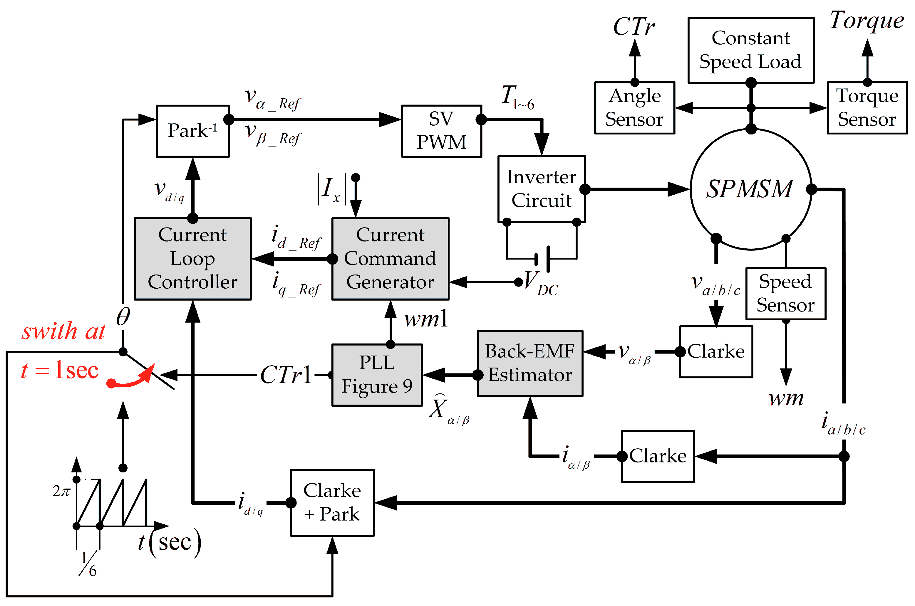
Figure 1 illustrates the proposed controller architecture, which is evaluated under a critical condition relevant to electric vehicle applications: power interruption during operation followed by system reboot, resulting in controller disconnection. Upon restarting, although the motor speed is at 300 rpm, sensorless operation necessitates an initial open-loop control at 360 rpm. After 1 s, the estimated output is injected into the system.

The estimation methods sequentially employed include the conventional sensorless scheme, the adaptive structure proposed by Shuo et al. [19], and the novel approach recommended in this paper. In this section (Stage I), only the first two methods are simulated to observe their behavior under such conditions. Stage II, detailed in Section 6, implements the proposed method to evaluate its potential contribution in addressing this application scenario.

It is important to note that, in the motor parameter settings listed in

Table 1. The list of the motor’s parameters used in the simulation.

$\mathrm{Stator} \mathrm{resistance},R_s$	$0.022 \mathrm{\Omega }$
Stator inductance on d- and q-axis, $L_d=L_q=L_s$	$0.22 \mathrm{mH}$
Number of poles, $P$	$8$
Peak line-to-line back EMF constant, $v$	$13.573{\displaystyle \frac{\mathrm{volts}}{\mathrm{krpm}}};$ Flux linkage, ${\lambda }_{PM}={\displaystyle \frac{60\cdot v}{\sqrt{3}\pi \cdot 1000P}}$
Moment of inertia, $J$	$1.79\times {10}^{-3} \mathrm{kg}\cdot {\mathrm{m}}^2$
Rating speed	$10 \mathrm{Krpm}$

, the instantaneous actual value of the stator inductance is denoted as $L_s=0.22 \mathrm{mH}$, whereas the controller algorithm utilizes a perturbed value of $0.23 \mathrm{mH}$. Furthermore, the simulation system is equipped with speed, position, and torque sensors to facilitate performance comparison.

During the simulation, the nomenclature is defined as follows: the actual motor speed and rotor position are represented by wm and CTr, respectively, while the corresponding estimated values from the control algorithm are denoted as wm1 and CTr1. The shaft torque is referred to as Torque.

To validate the proposed structure under practical conditions, PowerSIM 2023, a widely recognized simulation tool in the power electronics community, was employed. This platform enables system verification through piecewise mathematical modeling and facilitates the simulation of a complete sensorless control system within a unified environment.

As shown in Figure 10, the overall architecture shared by the three methods is presented. The differences lie in the shaded blocks, which are replaced according to the specific method being tested, while all other blocks utilize the built-in components of the simulation software.

The conventional back-EMF estimation combined with a PLL structure, as well as the adaptive super-twisting observer with an improved PLL proposed by Shuo et al. [19], were reconstructed for simulation purposes. The objective was to observe the behaviors of these two schemes under electric vehicle power interruption and reboot scenarios.

It is important to note that the reconstruction strictly adhered to the structural designs and parameter selections reported in [19].

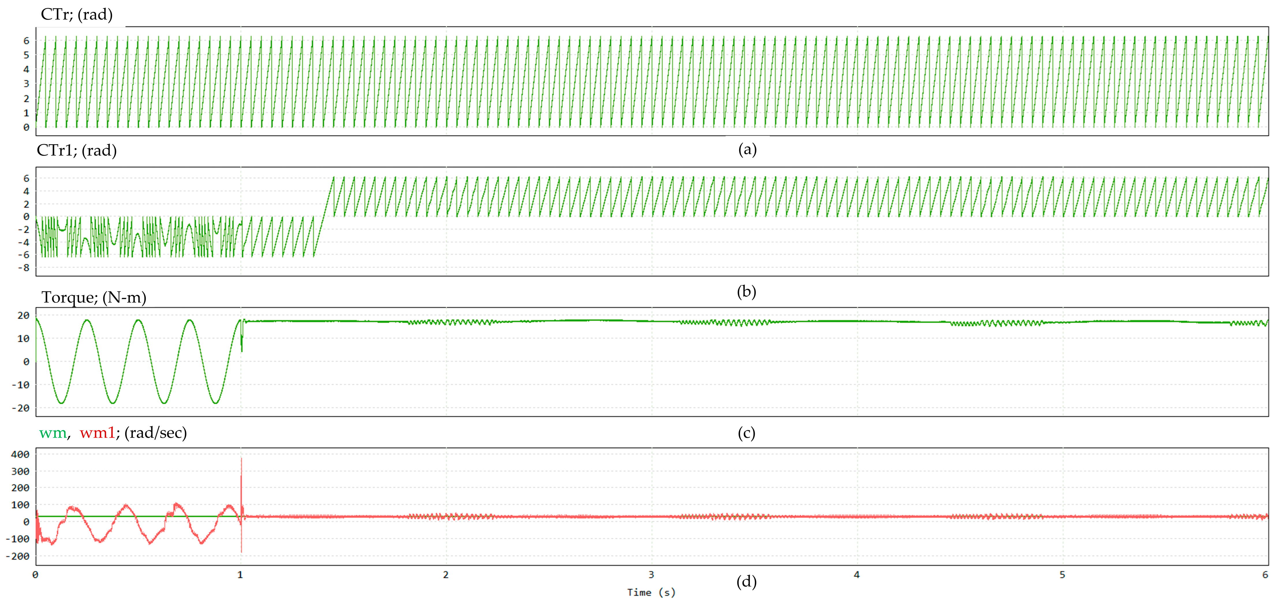
Figure 11 presents the simulation results of the conventional method. Subfigure (a) shows the actual rotor flux angle provided by the sensor, while (b) illustrates the estimated rotor flux angle obtained from the conventional algorithm. Subfigure (c) displays the shaft torque measured by the sensor, and (d) compares the actual rotor speed wm and the estimated rotor speed wm1.

As observed in Figure 11a, the rotor initially rotates at a constant speed. However, Figure 11b reveals that the estimated angle CTr1 not only fails to synchronize with the actual angle CTr but also exhibits an incorrect rotational direction. Injecting the estimated output into the system at 1 s does not improve the estimation accuracy. Simultaneously, persistent oscillations in the shaft torque are observed, as shown in Figure 11c. Although Figure 11d indicates that wm maintains a stable rotation at 31.4 rad/s, wm1 initially exhibits significant oscillations and ultimately converges to an incorrect rotational direction.

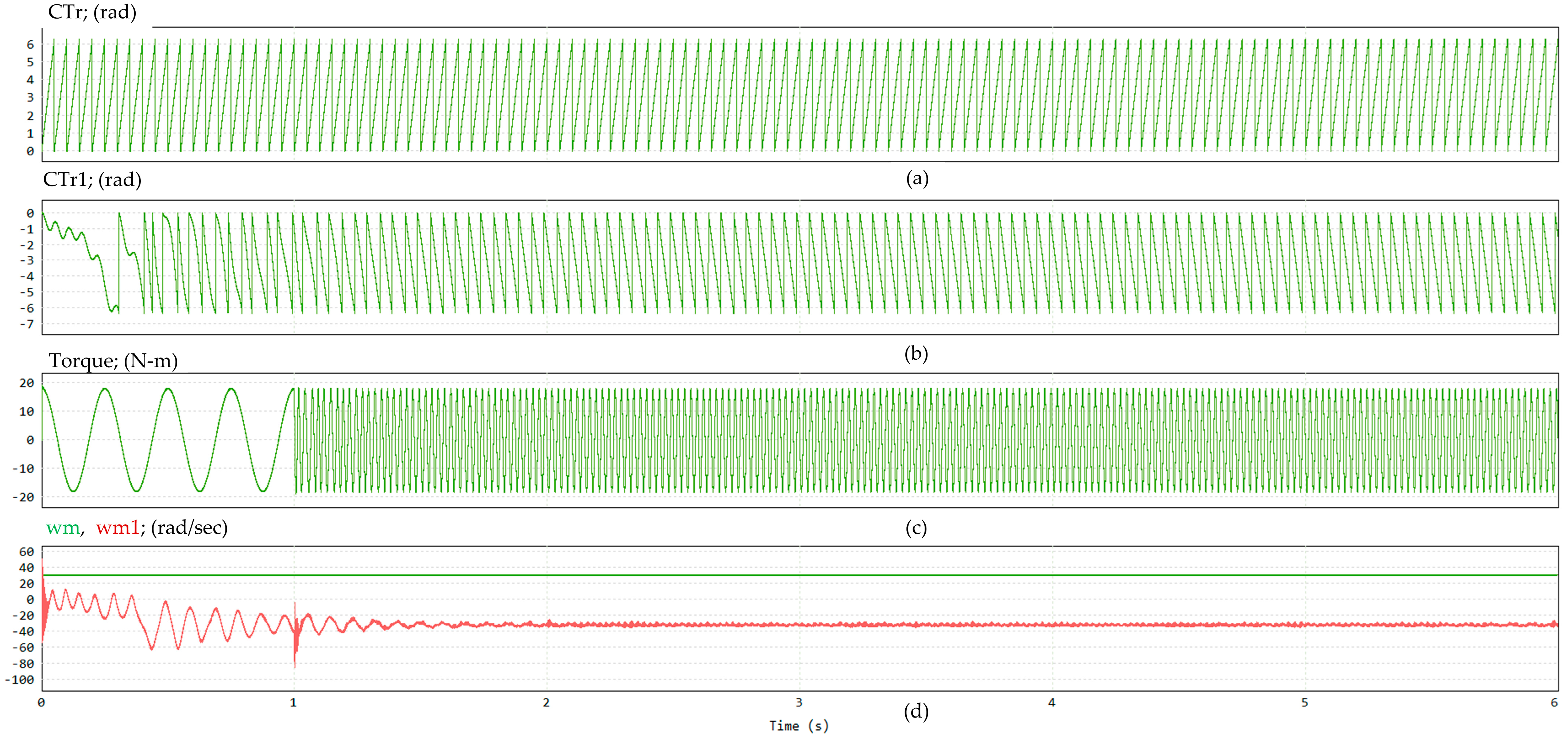
Figure 12 presents the simulation results based on the adaptive structure proposed by Shuo et al. [19]. Under the same testing scenario, the performance is significantly improved compared to the conventional method. From the beginning of the process, the estimated rotor flux angle CTr1 gradually converges toward the actual angle CTr. After injecting the estimated output into the system at 1 s, noticeable tracking behavior is observed, although the convergence progresses slowly.

During the tracking phase, the shaft torque continues to exhibit oscillations until the estimated angle and speed synchronize with their actual counterparts. Torque stabilization is achieved approximately 5 s after the estimated values are injected. As shown in Figure 12c, the peak torque initially reaches nearly 20 N·m, but the final steady-state torque falls below 10 N·m, indicating a significant underestimation.

5. The Parameter Self-Tuning Algorithm

The results obtained thus far still indicate considerable room for improvement, particularly for electric vehicle applications. Therefore, beyond the first-stage enhancement involving modifications to the PI regulator within the PLL, a second-stage improvement is proposed in this work, namely a gradient-based self-tuning algorithm.

In sensorless control, by definition, no feedback other than voltage and current measurements is available; thus, no information regarding shaft dynamics can be directly obtained. Inspired by the analysis shown in Figure 4, it is observed that $\Delta i_{\alpha }$ and $\Delta i_{\beta }$ are known quantities, both influenced by the estimated inductance parameter ${\stackrel{⌢}{L}}_s$.

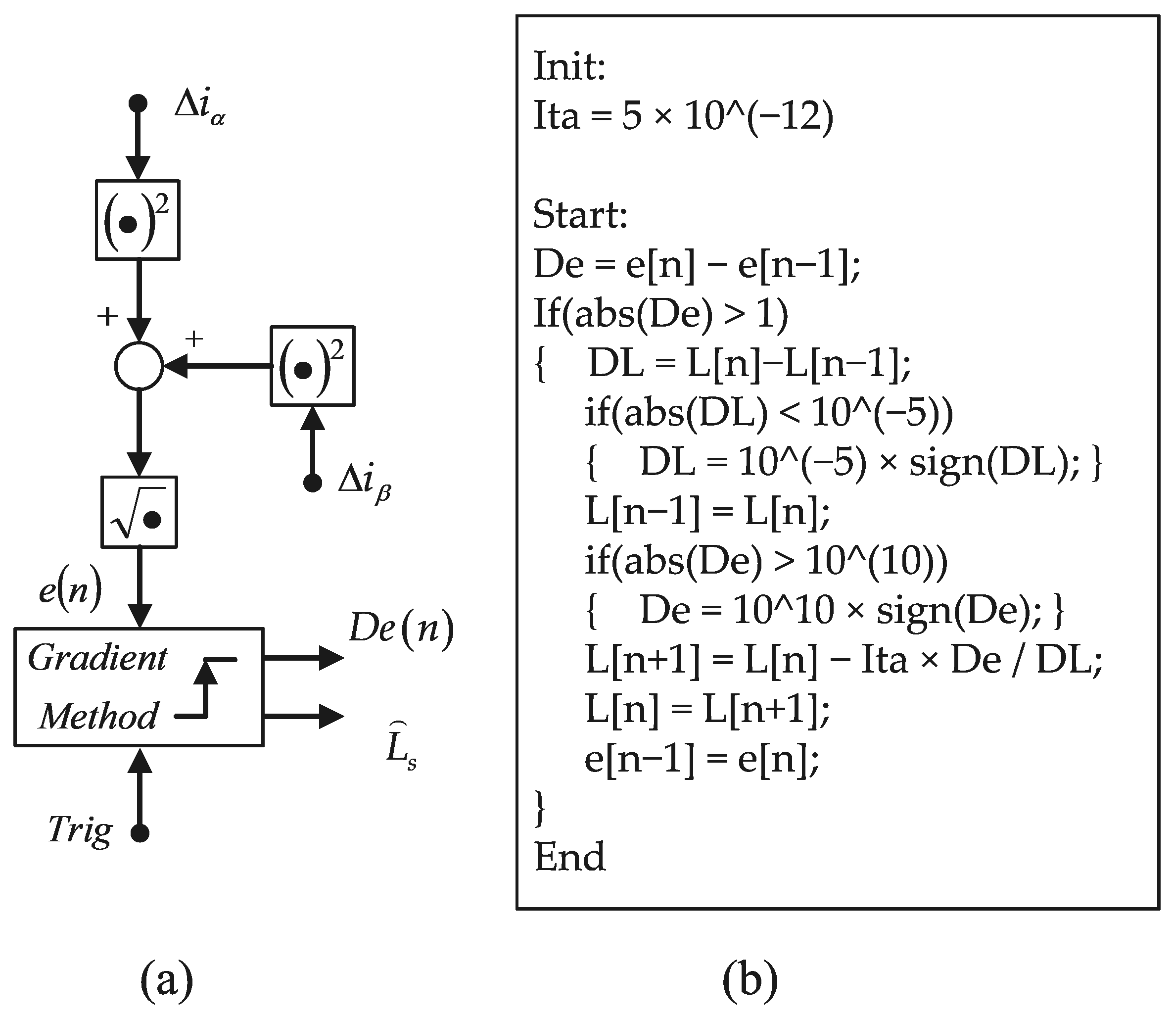
Based on this observation, Figure 13 illustrates a constructed structure wherein the magnitude of the vector sum of $\Delta i_{\alpha }$ and $\Delta i_{\beta }$ is indicated as follows:

$$e=\sqrt{\Delta i_{\alpha }^2+\Delta i_{\beta }^2}$$

(22)

serving as an indicator of the consistency between the actual and estimated inductance values. This relation subsequently triggers the activation of the gradient-based adjustment mechanism.

The detailed operation of the gradient adjustment mechanism is described as follows. Upon the rising edge of the trigger signal (Trig), the gradient adjustment process is initiated. The Trig period is set to approximately 1/1000 of the system control period to avoid frequent parameter updates, which could otherwise destabilize the system and increase computational burden. The detailed implementation can be referred to in the code example shown in Figure 13b.

Specifically, this adjustment follows:

$${\stackrel{⌢}{L}}_s\left(n+1\right)={\stackrel{⌢}{L}}_s\left(n\right)-\eta {\displaystyle \frac{e\left(n\right)-e\left(n-1\right)}{{\stackrel{⌢}{L}}_s\left(n\right)-{\stackrel{⌢}{L}}_s\left(n-1\right)}},$$

(23)

where $\eta$ denotes the step size, also referred to as the learning rate. This parameter plays a critical role in determining the convergence behavior of the algorithm. If $\eta$ is set too small, convergence becomes excessively slow, prolonging the adaptation time. Conversely, if $\eta$ is too large, the iteration may become unstable and even diverge due to overshooting. Therefore, careful selection of the step size is essential and should be based on the specific characteristics of the application.

In addition, attention must be given to the conditions associated with $\left|De\right|$ and $\left|DL\right|$. If $\left|De\right|$ becomes sufficiently small, indicating convergence, the self-adjustment process can be suspended. Conversely, if $\left|DL\right|$ falls below a certain minimum threshold, indicating potential divergence, a safeguard mechanism must be activated to prevent instability.

6. Stage II of the Simulation

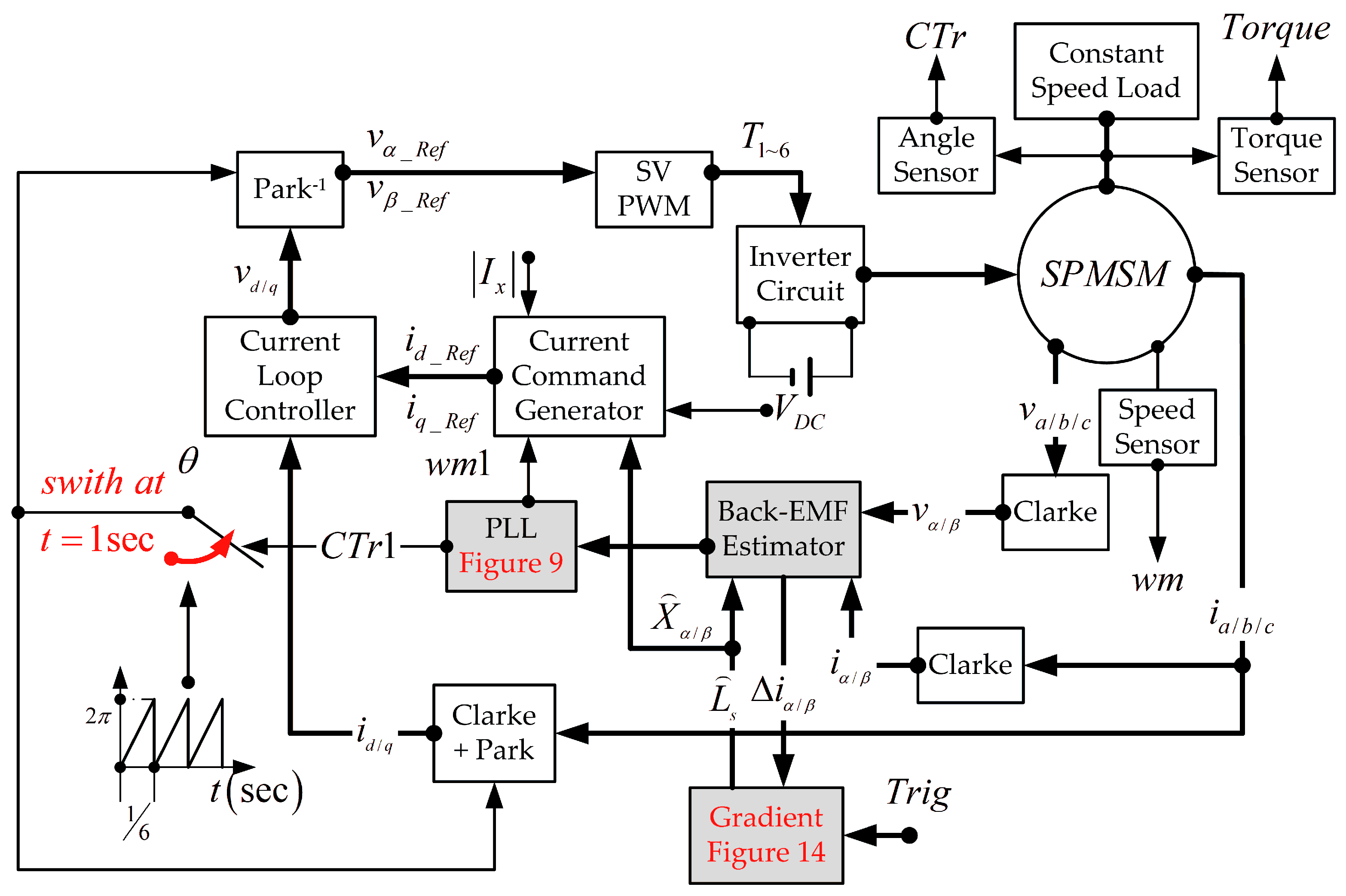
The proposed improvement scheme has been integrated into the original control framework, as illustrated in Figure 14. Specifically, the gradient computation block utilizes the intermediate signals $\Delta i_{\alpha }$ and $\Delta i_{\beta }$ from the back-EMF estimator. Upon the triggering of the Trig signal, the block generates the updated estimate ${\stackrel{⌢}{L}}_s$, which is immediately iteratively fed back into the system.

Furthermore, the update interval for adjusting ${\stackrel{⌢}{L}}_s$ using the gradient method must be sufficiently long. This requirement arises because the system response inherently lags behind the instantaneous variation in ${\stackrel{⌢}{L}}_s$. If the parameter updates are performed too frequently, the estimation process may respond to transient effects rather than the actual steady-state behavior, resulting in erroneous adjustments based on $e\left(n\right)$. Therefore, an appropriate update period must be selected to allow the system sufficient time to reflect the impact of each parameter modification before subsequent updates are applied.

The pseudocode presented below illustrates the sensorless control algorithm for the permanent magnet synchronous motor (PMSM) proposed in this paper, incorporating back-EMF estimation, parameter self-tuning, and an enhanced phase-locked loop (PLL):

• Inputs: initial parameters, including the estimated stator inductance (${\stackrel{⌢}{L}}_{s0}$) and stator resistance ($R_s$).
• Outputs: estimated rotor speed (${\stackrel{⌢}{\omega }}_{rf}$), rotor position (${\stackrel{⌢}{\theta }}_{rf}$), and updated parameters (${\stackrel{⌢}{L}}_s$).
• Initialization:

  ⚬

  Set the initial motor parameters: $R_s$ (stator inductance estimate) and ${\stackrel{⌢}{L}}_{s0}$ (initial inductance estimation).

  ⚬

  Define the PLL parameters, including the loop gain ($\begin{array}{cc}{K}_1,& K_2\end{array}$).

  ⚬

  Define the adaptive parameters, including the learning rate ($\eta$) and the update interval ($T_s$).

  ⚬

  Start the motor using open-loop control.

• Main Loop (executed at each control cycle; $T_s$):

  ⚬

  Measure the stator voltages $\begin{array}{cc}{v}_{\alpha },& v_{\beta }\end{array}$ and currents $\begin{array}{cc}{i}_{\alpha },& i_{\beta }\end{array}$.

  ⚬

  Estimate the back-EMF signals based on the measured quantities.

  $$\begin{gathered} {\stackrel{⌢}{X}}_{\alpha }\left(n\right)=v_{\alpha }\left(n\right)-R_s{i}_{\alpha }\left(n\right)-{\stackrel{⌢}{L}}_s\left(n\right)\left[i_{\alpha }\left(n\right)-i_{\alpha }\left(n-1\right)\right]{\displaystyle \raisebox{1ex}{$1$}\!\left/ \!\raisebox{-1ex}{$T_s$}\right.}, \\ {\stackrel{⌢}{X}}_{\beta }\left(n\right)=v_{\beta }\left(n\right)-R_s{i}_{\beta }\left(n\right)-{\stackrel{⌢}{L}}_s\left(n\right)\left[i_{\beta }\left(n\right)-i_{\beta }\left(n-1\right)\right]{\displaystyle \raisebox{1ex}{$1$}\!\left/ \!\raisebox{-1ex}{$T_s$}\right.} \end{gathered}$$

  ⚬

  Rotor Flux Angle Estimation Error Calculation:

  $$\stackrel{⌢}{\epsilon }\left(n\right)={\stackrel{⌢}{X}}_{\alpha }\left(n\right)\sin \left[{\stackrel{⌢}{\theta }}_{rf}\left(n\right)\right]-{\stackrel{⌢}{X}}_{\beta }\left(n\right)\cos \left[{\stackrel{⌢}{\theta }}_{rf}\left(n\right)\right]$$

  ⚬

  Rotor Position ${\stackrel{⌢}{\theta }}_{rf}$ and Speed ${\stackrel{⌢}{\omega }}_{rf}$ Update Using Enhanced PLL:

  $$\begin{gathered} y\left(n\right)=K_1\stackrel{⌢}{\epsilon }\left(n\right)-K_{2}x\left(n-1\right), x\left(n\right)=x\left(n-1\right)+\left[y\left(n\right)+y\left(n-1\right)\right]{\displaystyle \raisebox{1ex}{$T_s$}\!\left/ \!\raisebox{-1ex}{$2$}\right.}, \\ {\stackrel{⌢}{\theta }}_{rf}\left(n\right)={\stackrel{⌢}{\theta }}_{rf}\left(n-1\right)+\left[x\left(n\right)+x\left(n-1\right)\right]{\displaystyle \raisebox{1ex}{$T_s$}\!\left/ \!\raisebox{-1ex}{$2$}\right.}. \end{gathered}$$

The signal ${\displaystyle \frac{1}{T_s}}\left[{\stackrel{⌢}{\theta }}_{rf}\left(n\right)-{\stackrel{⌢}{\theta }}_{rf}\left(n-1\right)\right]$ is processed through a low-pass filter to obtain the filtered output $\to {\stackrel{⌢}{\omega }}_{rf}\left(n\right)$.

• Parameter ${\stackrel{⌢}{L}}_s$ Self-Tuning Loop (triggered every $1000\times T_s$ cycles):

  ⚬

  Current Estimation Error Variation Calculation: $De=e\left(n\right)-e\left(n-1\right)$.

  ⚬

  If $\left|De\right|>1$, update inductance; otherwise, exit the adaptation process.

  ⚬

  If $\left|DL\right|<{10}^{-5}$, $\left|DL\right|={10}^{-5}\times \mathrm{sgn}\left(DL\right)$.

  ⚬

  If $\left|De\right|>{10}^{10}$, $\left|De\right|={10}^{10}\times \mathrm{sgn}\left(De\right)$.

  ⚬

  Update the inductance parameter using the gradient descent method based on (23).

  ⚬

  State update for next iteration.

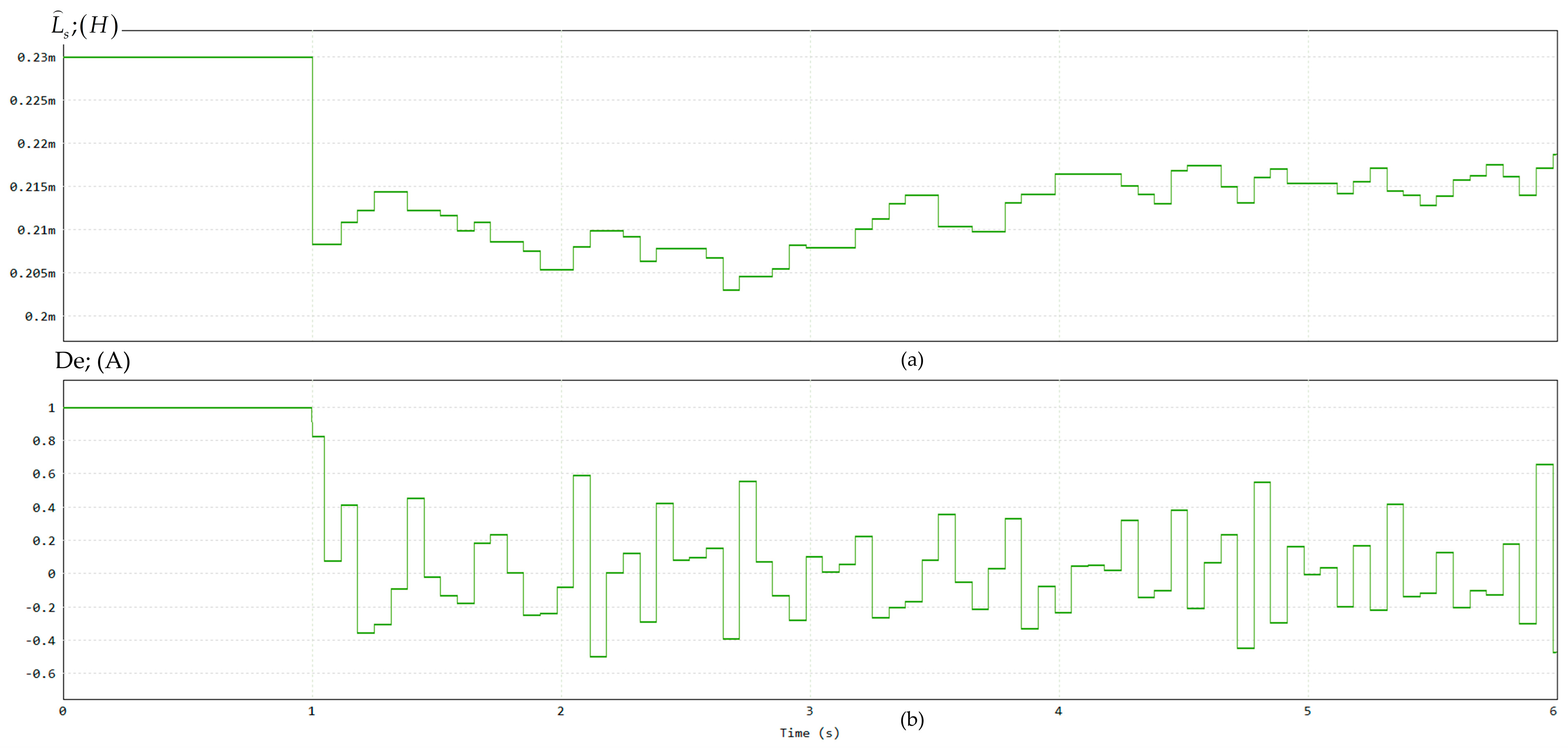
Based on the same simulation procedure, Figure 15a illustrates that the originally distorted system parameter (stator inductance ${\stackrel{⌢}{L}}_s$) can be adaptively tuned from 0.23 mH to 0.22 mH. The current estimation error (De) plays a critical role in this adaptation process. After the estimation is applied, De remains consistently at a low level throughout the operation, as shown in Figure 15b.

Figure 16 demonstrates the superior performance of the proposed method. After feeding back the estimated outputs into the control computation, the speed tracking rapidly converges, and the shaft torque stabilizes immediately. Within approximately 0.5 s, the rotor flux angle tracking is completed. Moreover, as shown in Figure 16c, the stabilized shaft torque almost recovers to its peak value, indicating effective disturbance rejection and dynamic performance restoration.

7. Conclusions

This paper proposes replacing the traditional PI controller within the PLL structure with a zero-free PI regulator, coupled with a gradient-based parameter self-tuning module. After conducting simulations under three different computational frameworks, it was observed that non-steady-state starting conditions, such as power-off restart scenarios, can cause the conventional sensorless operation (Figure 11) to fail. Furthermore, although the improved method proposed by Shuo [19] provided noticeable enhancements under the same conditions (Figure 12), the performance was still not fully satisfactory for demanding applications.

To address this issue, this paper proposes replacing the traditional PI controller within the PLL structure with a zero-free PI regulator, coupled with a gradient-based parameter self-tuning module. Simulation results demonstrate that the proposed method significantly improves robustness, effectively suppresses signal oscillations, and maintains stable operation even under challenging dynamic conditions.

It is worth emphasizing that the proposed gradient-based self-tuning module effectively utilizes intermediate variables from the back-EMF observer to tightly track the variations in the actual stator inductance (${\stackrel{⌢}{L}}_s$). Importantly, this approach maintains the sensorless constraint, requiring only the terminal voltages and currents of the motor without the need for any shaft-based motion feedback.

The simulation results validate the effectiveness of combining the proposed PLL structure with the recommended parameter self-tuning scheme. This approach not only enhances the stability of the sensorless control system but also improves estimation accuracy and dynamic performance, demonstrating its suitability for practical permanent magnet synchronous motor (PMSM) drive applications.

Furthermore, the combined computational framework has been verified on actual electric vehicles, where enhanced robustness, stability, and accuracy were consistently observed under various operating conditions, confirming the practical viability of the proposed method.