Abstract
Virtual coupling (VC) technology, which determines the safe interval between trains based on relative braking distance, offers a promising solution by enabling tighter yet safe train-following intervals through advanced communication and control strategies. This paper focuses on addressing the virtually coupled train set (VCTS) control problem within the framework of distributed model predictive control (DMPC), in which train dynamics model incorporates uncertainties in basic resistance and control inputs, with an adaptive mechanism (ADM) designed to limit errors caused by external disturbances. A multi-objective cost function is established, considering position error, speed error, and ride comfort, while constraints such as actuator saturation, speed limits, and safe tracking distance are enforced. Particle swarm optimization (PSO) is employed to solve the non-convex optimization problem globally. Simulation experiments validate the effectiveness of the proposed method, demonstrating stable operation of VCTS under various initial conditions and the ability to handle uncertainties through the adaptive mechanism. The results show that the proposed DMPC approach significantly reduces tracking errors and improves ride comfort, highlighting its potential for enhancing railway capacity and operational efficiency.
Keywords:
virtual coupling; virtually coupled train set; distributed model predictive control; adaptive control; particle swarm optimization MSC:
93B45
1. Introduction
With the rapid growth of railway transportation demand, how to further enhance line capacity and operational efficiency while ensuring safety remains an enduring pursuit for railway operators. One of the critical bottlenecks restricting line capacity is the signaling system, as its protection mechanism directly determines the spacing between trains [1]. Currently, the most advanced signaling system in practical engineering applications is the moving block system, which determines the safe interval between two trains based on the absolute braking distance of the following train [2]. This mechanism does not consider the speed of the leading train, assuming instead that the leading train could come to an instantaneous stop. However, during train-following operations, the position of the leading train continuously moves forward, leaving room for further compression of the tracking interval between adjacent trains. Optimizing this interval through advanced control strategies and dynamic signaling adjustments could unlock significant potential for improving line capacity and operational efficiency [3].
Virtual coupling (VC) [4] technology further enhances line capacity by determining the safe interval between adjacent trains based on relative braking distance, building upon the foundation of the moving block system [5]. Unlike traditional mechanical coupling, virtual coupling employs train-to-train (T2T) communication to establish a virtual connection between trains in a virtually coupled train set (VCTS). By dynamically adjusting the spacing between trains in real time and leveraging advanced communication and control strategies, virtual coupling enables tighter yet safe train-following intervals, thereby maximizing line capacity and operational efficiency while maintaining high safety standards.
With the advancement of communication and computer technologies, the practical implementation of virtual coupling has become feasible, and virtual coupling train control technology has emerged as a prominent research focus in recent years. Xun et al. [6], Wu et al. [7], and Felez et al. [8] provided a comprehensive review of virtual coupling train control technologies, highlighting that numerous advanced control methodologies, such as intelligent control [9], stochastic control [10], model predictive control [11], optimal control [12], sliding mode control [13], and consensus-based control [14], have been successfully employed to tackle the VCTS control. This paper focuses on addressing the VCTS control problem within the framework of model predictive control, owing to its advantages in predicting system behavior, interference resistance, and its ease of extensibility.
Model predictive control (MPC) is an advanced control strategy based on the dynamic model, rolling-horizon optimization, and feedback correction. Its core principle lies in utilizing a mathematical model of the system to predict its behavior over a future time horizon and optimizing the control inputs accordingly, ensuring that the system achieves optimal performance while satisfying constraints [15].
Felez et al. [16] proposed a nominal MPC framework for each train in a VCTS. The control strategy was compared to the traditional moving block train control system. The study focused on a metro line scenario, demonstrating that virtual coupling significantly reduces the headway and distance between trains. Based on this work, Felez et al. [17] developed a robust MPC approach that incorporates two types of uncertainties in the controller, i.e., train positioning errors and adhesion losses. In addition, more undetermined disturbances, such as resistive modeling errors and communication delays, were considered in reference [18]. Liu et al. [19] presented a distributed MPC framework for VCTS, where a terminal constraint set and terminal controller are explicitly designed to ensure both feasibility and stability of the control system. A comparative evaluation of cooperative distributed MPC, serial distributed MPC, and decentralized MPC in addressing the control performance of VCTS was conducted in reference [20], taking into account the heterogeneous characteristics of trains. The stability of the proposed control methods was analyzed using the relaxed dynamic programming approach. Luo et al. [21] addressed the control challenges of VCTS in dynamic environments by proposing an adaptive model predictive control method. A train dynamics model estimator incorporating a variable-step descent algorithm was designed to acquire accurate parameters in time-varying environments. Furthermore, Luo et al. [22] introduced a serial distributed robust MPC approach to achieve close-following operation for VCTS. A controller-tuning algorithm based on semi-definite programming was developed, and a terminal constraint set was created to ensure the recursive feasibility in closed-loop implementation.
In summary, most of the previous studies have considered model uncertainties, but few have simultaneously accounted for uncertainties in both resistance and control inputs. This gap is critical because resistance forces and actuator limitations jointly constrain the train dynamic model [23]. Furthermore, the cost functions in the literature predominantly focus on single objectives such as tracking error or tracking distance, with limited consideration of other performance in virtual coupling train control, such as ride comfort. Regarding the solution of optimization problems, existing research primarily relies on numerical optimization methods, e.g., sequential quadratic programming. However, for nonlinear, non-convex, or high-dimensional problems, these methods may suffer from local optima or low computational efficiency. Compared to the existing literature, a novel distributed model predictive control (DMPC) approach for VCTS control is presented. The contributions of this paper can be summarized as follows:
- The train dynamics model incorporates uncertainties in basic resistance and disturbances in control inputs. Specifically, an adaptive mechanism (ADM) is constructed to limit errors caused by external unknown disturbances, bringing the model closer to the real state.
- For the rolling optimization problem within the DMPC framework, a multi-objective cost function is established, considering position error, speed error, and ride comfort. Constraints such as actuator saturation, speed limits, and the nonlinear coupled constraint of safe tracking distance are also taken into account.
- Particle swarm optimization (PSO) is integrated into the DMPC framework to search for the optimal control input sequence, enabling global optimization of the formulated non-convex problem.
The rest of this paper is organized as follows. Section 2 provides a detailed description of the VCTS control problem from three aspects: the train dynamics model, system constraints, and state-space representation. Section 3 elaborates on the designed control method, including an ADM for handling uncertainties and a PSO-based global optimization solver, along with a theoretical stability analysis of the controller. Section 4 validates the performance and effectiveness of the proposed method through simulation experiments. Finally, Section 5 concludes the paper by summarizing the research findings and outlining potential directions for future work.
2. Problem Description
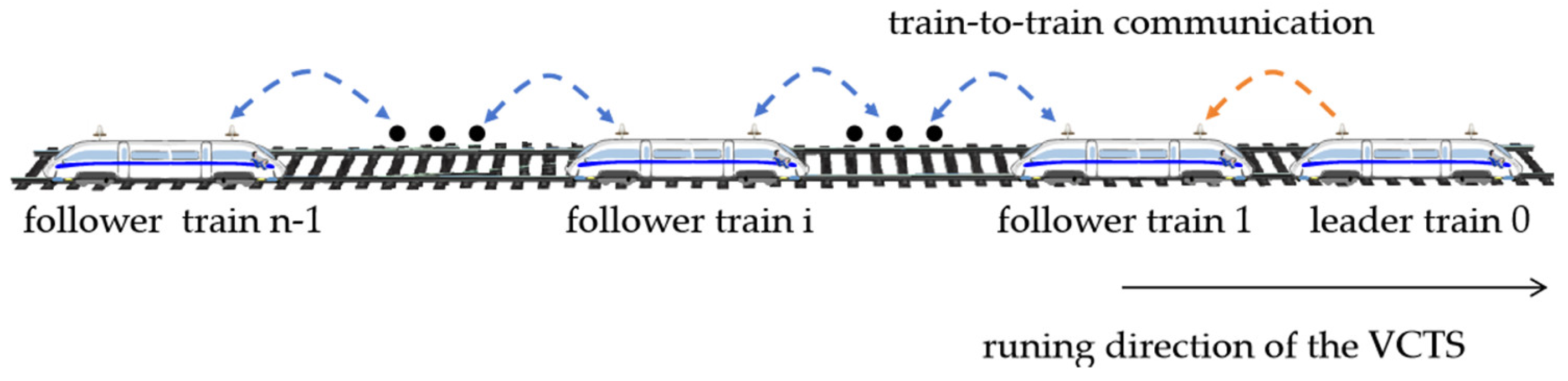
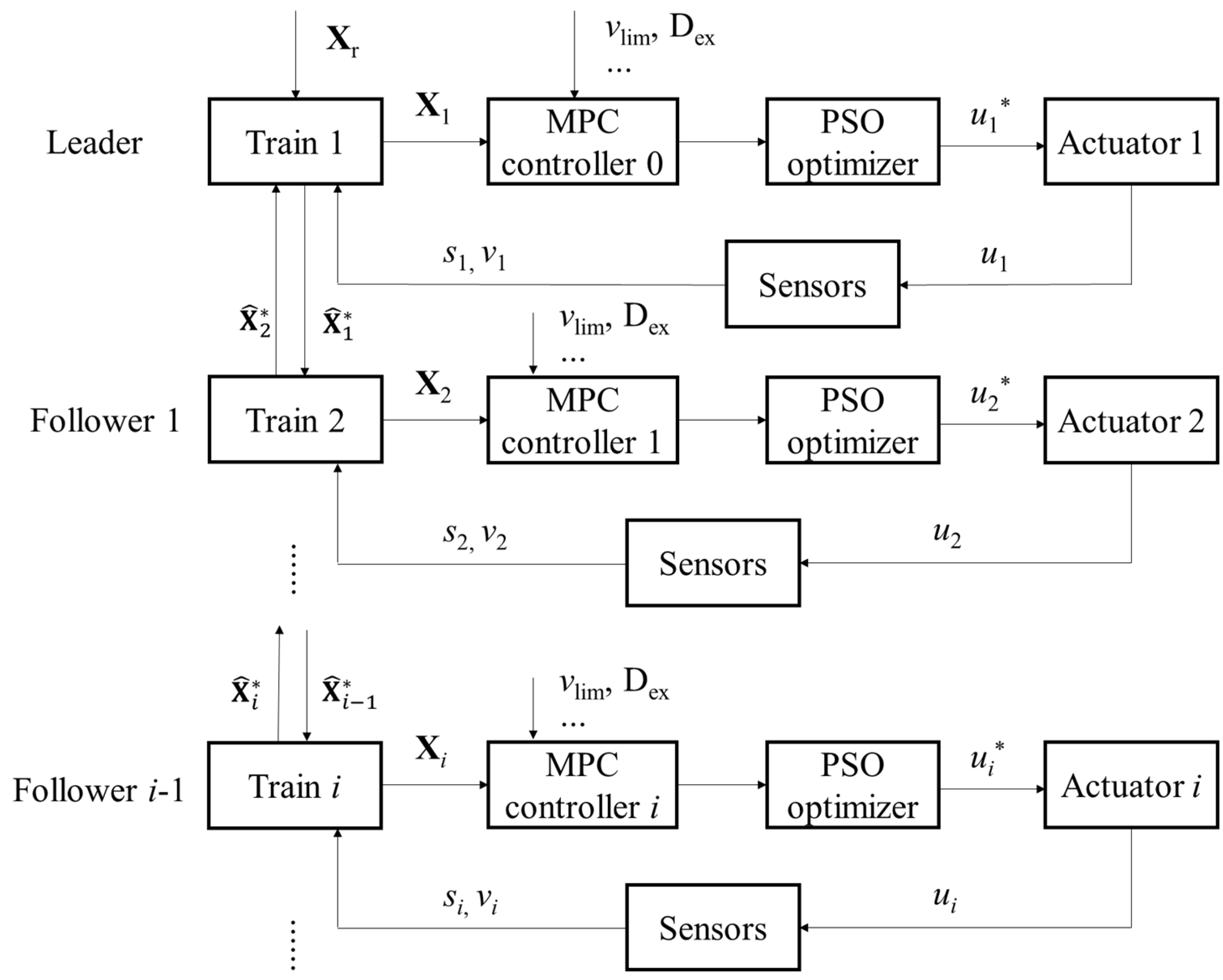
Let us define a VCTS with T2T communication, consisting of trains and adopting a distributed control architecture. Its structural composition and communication topology are illustrated in Figure 1. The coordination within the VCTS is achieved through a leader–follower relationship, where the first train in the direction of the train running is regarded as the leader, with the index , while the remaining trains act as followers, with the index . Each train is equipped with its own controller, which obtains information such as position, velocity, and acceleration through onboard devices and shares its state with adjacent trains. The leader train tracks the predefined reference trajectory and unidirectionally transmits its state information to its follower train. Meanwhile, bidirectional communication among follower trains enables adaptive cooperative control through mutual state exchange.
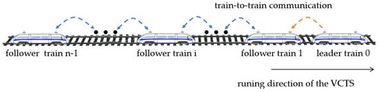
Figure 1.
Structural composition and communication topology of the VCTS.
2.1. Train Dynamics Model
The train dynamic model serves as the fundamental basis for the design and optimization of train control systems, particularly in complex operational scenarios such as virtual coupling. The longitudinal motion of a train is influenced by multiple factors, including traction and braking forces, basic resistance (rolling and bearing resistances, aerodynamic drag), and additional resistance (external forces due to track grade, curvature, and tunnel). Based on the longitudinal dynamics of the train, a single-point mass model is established, such model not only incorporating the fundamental equations of motion, but also accounting for system uncertainties.
The train dynamics model is described as follows:
where , , and represent the position, velocity, and traction/braking force of train at timestamp , respectively. The term denotes the mass of train . represents the basic resistance per unit mass of the train which is dependent on the train’s structure and operating speed, and signifies the additional resistance per unit mass of the train which is influenced by the conditions of the railway line.
The basic running resistance can be calculated using the Davis formula, which is given in Equation (2):
where , , and are Davis coefficients, which are empirically derived based on practical experience.
The additional resistance, , consists of resistances due to the track grade (), track curves (), and tunnels () [7], and it can be denoted as follows:
where , , and represent the track grade, the radius of track curves, and the length of tunnels, respectively.
The aforementioned train dynamic model serves merely as a nominal representation, wherein the basic running resistance parameters and control inputs are derived from experimental and testing procedures under specific conditions. However, these parameters are subject to external and internal disturbances under varying operational conditions of the train, such as adverse weather conditions (e.g., strong winds) and performance degradation in electrical motors. Consequently, the actual train dynamic model exhibits inherent uncertainties due to these perturbations. In such cases, the basic running resistance and control input can be rewritten as follows:
where , , and represent the disturbances in the respective components of the Davis equation, while denotes the disturbance in the control input.
2.2. Independent and Coupled Constraints
The operational performance of VCTS is constrained by a variety of complex factors, including variations in operating conditions, the inherent dynamic characteristics of the trains, and stringent requirements for safe spacing. These factors impose strict limitations on the state variables and control inputs of the trains. To ensure that VCTS operates efficiently while meeting safety and comfort requirements, it is essential to thoroughly incorporate these constraints into the train dynamic model.
Constraints 1.
The control inputs of the traction and braking systems of trains must satisfy the limitations imposed by hardware and actuators, such limitations can be denoted as follows:
where and represent the maximum breaking force and maximum traction force, respectively.
Constraints 2.
The train speed must not exceed the fixed line speed limits or the temporary speed limits issued by the dispatcher and can be expressed as follows:
where is the speed limit at the current position of the train.
Constraints 3.
During the operation of a VCTS, adjacent trains maintain an expected spacing based on the principle of relative braking distance. The coupling constraints between the trains are described as follows:
where is the length of the preceding train and is the expected spacing between adjacent trains, such spacing being related to the braking distance of the trains and the safety margin redundancy. It can be expressed as follows:
where
is a user-defined safety margin redundancy and
is the distance required for the train to brake to a complete stop from its current speed, a parameter that can be denoted as follows:
where denotes the emergency braking acceleration of the train.
2.3. State–Space Representation
The state of train in the VCTS is defined as follows:
To better express the train state transition process, we transfer Equation (1) to the train state–space transition equation as follows:
where
Actually, it is difficult to estimate every parameter in . Therefore, we consider the train model as a whole for the convenience of modeling establishment and simulation test execution. Furthermore, the state transition equation of the train is derived by substituting Equation (4) into Equation (12) and simplifying, as follows:
where
3. DMPC Framework
In the proposed DMPC framework, both the leader train and each follower train are equipped with independent controllers, and the state information is exchanged in real-time through T2T communication to dynamically optimize control strategies. The controller solves an optimal control problem over a finite time horizon based on a known train dynamics model, generating an optimal control input sequence over time. To adapt to the changes in the operating environment and meet real-time control requirements, the controller only applies the first control input in each optimization cycle. It is worth noting that the optimization objectives of the leader train and the follower trains are different: the controller of the leader train aims to track a predefined reference trajectory, minimizing speed and distance tracking errors to zero, while the follower trains aim to synchronize their speed with the preceding train and maintain a relatively safe following distance.
3.1. Controller Design
In the DMPC architecture, the running state of train over a prediction horizon is defined as follows:
where denotes the predicted train state information of t + 1 at time t.
Combining Equations (13) and (14), the state–space transition equation in DMPC can be expressed as follows:
where
Due to the influence of external disturbances, the train model matrix becomes time-varying. Therefore, this paper proposes an ADM, expressed as follows:
where represents the deviation between the real train model and the nominal one.
In this study, the tracking error of train states and ride comfort are taken as optimization objectives of VCTS control, and the cost function is defined as follows:
where represents the state vector of train in terms of distance and velocity, a variable that can be expressed as follows:
where , , and are weight matrices, which can be expressed as follows:
, , , , , are weight values of the tracking speed error, tracking distance error, and comfort, respectively. and are weight values of the tracking speed error and tracking distance error of train (i + 1), respectively.
For the leader train, denotes the reference running trajectory, while for the follower trains, represents the state vector of adjacent trains which can be expressed as follows:
Comfort is reflected by the jerk of the train and can be expressed as follows:
where represents the acceleration of train I and denotes the time step.
The optimal control sequence within the prediction horizon that the DMPC controller obtains can be expressed as follows:
The control input for train at time is as follows:
MPC adopts a rolling horizon strategy, meaning that, within each control cycle, only the first control input obtained from optimization is executed within each control cycle. Thus, the proposed control scheme with the ADM in a rolling horizon is shown in Figure 2.
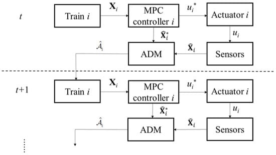
Figure 2.
The control scheme with the ADM in a rolling horizon.
3.2. Controller Convergence Analysis
The convergence analysis of the controller is a critical step to ensure that the designed control method can achieve a stable state within a finite time. The goal of the controller is to optimize the control input such that the systematic model converges to the actual one, while satisfying the system constraints.
Remark 1.
During the execution of the controller for train at time , the estimated parameter matrix
, remains constant within each prediction horizon.
The objective of the ADM for train is to minimize the deviation between the predicted state and the actual state at time , and can be expressed as follows:
where , then Equation (24) can be rewritten as follows:
By calculating the gradient of the above formula with respect to the estimated parameter matrix , the following equation is obtained:
We expect the estimated train state to gradually converge to the true state through the gradient descent direction. Therefore, the update strategy for the train model matrix can be described as follows:
Theorem 1.
There exists a step size, , such that the estimated train model matrix,
, of the train dynamic model converges to a bounded matrix
, after a finite amount of time.
Proof of Theorem 1.
A Lyapunov function related to the estimated train model matrix of the train model is designed as follows:
By combining Equation (28) with Equation (27), we obtain the following equation:
Furthermore, the above equation can be rewritten as follows:
Due to , as long as the step size, , satisfies
can be achieved, thereby ensuring the asymptotic convergence of the train model parameters. If the initial value , of the aforementioned Lyapunov function is bounded, then as time approaches infinity , is also bounded. □
Therefore, based on Equation (31), the update step size for the train model matrix is designed as follows:
where .
Lemma 1.
As time approaches , the prediction error of the train state tends to zero, i.e., .
Proof.
Substituting Equation (32) into Equation (30), starting from , the expression can be written sequentially as follows:
By summing the left-hand side and the right-hand side of the above equations separately, we obtain the following:
After substituting Equation (32) into Equation (34), we obtain the following:
Since , the following is true:
Then, we obtain the following:
From Theorem 1, it is known that, as time approaches infinity , is bounded, and thus is also bounded. According to Equations (6)–(8), it can be concluded that the train state is always bounded. Therefore, is also bounded, and as time approaches infinity, tends to zero. □
3.3. Algorithm Design
MPC determines the optimal control input sequence by solving an optimization problem. Since Equation (17) is a high-dimensional cost function for multi-objective optimization, there may exist multiple local optima, and traditional methods such as the interior point method and sequential quadratic programming may converge to a suboptimal solution. Particle swarm optimization, a powerful swarm intelligence optimization algorithm, is characterized by its simple structure, fast convergence, and high precision, making it widely used for online parameter optimization. Furthermore, several studies have demonstrated that applying the PSO algorithm to solve MPC problems can yield favorable results [24,25,26]. Therefore, in the proposed DMPC-based virtual coupling train controller, the PSO algorithm is employed to perform global optimization of the cost function.
The velocity and position of particle are updated according to the following equation:
where denotes the inertia coefficient, and are preset learning parameters, and and are the m-th individual best value and global best value of the population at r-th iteration, respectively.
To expand the global searching scope of PSO in the early iteration time, while increasing the local optimizing speed later, is designed dynamically as follows:
where and are the preset maximum and minimum inertia coefficient, respectively.
To retain a reasonable searching speed and scope at each period, we design a bound mechanism for and as follows:
where and represent the minimum and maximum searching speed, respectively, while and are the minimum and maximum updating range, respectively.
According to Equation (17), the cost function represents the tracking error and jerk error, meaning that a lower value is the better individual. Thus, we design the individual and global best value selection mechanism in a PSO iteration range as follows:
where and are the minimum cost values of the m-th individual and the whole population, respectively.
The PSO-based DMPC framework is illustrated in Figure 3, and the steps of the proposed VCTS control method are detailed in Algorithm 1.
| Algorithm 1 Algorithm for the VCTS control |
| Input: train state–space
, , , estimated train model line conditions (slope, curve, tunnel), speed limit, and other necessary parameters for the MPC controller and the PSO optimizer. Output: train state–space , estimated train model . Procedures: 1. Agent and environment initialization: initialize train model parameters , line conditions, line speed limit distribution, reference profile, and PSO optimizer parameters. 2. MPC controller process: (a) Controller initialization: set the horizon Np, the population Ng, the learning rates c1 and c2 for personal best value and global best value, respectively, and the inertial coefficient . (b) State prediction: utilize to generate a series of control inputs and predict a predicted a series of train state for all individuals. (c) PSO process: (1) Cost calculation: calculate the cost values for all individuals according to Equation (17). (2) Best choosing: update the personal best values and global best value according to Equations (41) and (42). (3) Coefficient update: calculate the updated control input for all individu-als in the next iteration time according to Equations (38) and (40). (4) Back to step (b) until the optimization process reaches the maximum it-eration time, Nr. (d) State update: utilize and the optimal predicted control input to calculate the predicted train state information at time (t + 1). 3. Train model update: compare the predicted train state information and the theoretical train state information and update the train model to a new one at time (t + 1), according to Equation (27). 4. Back to step 2 until the train reaches the destination of the simulation process. 5. Result output: record the train state information of every time step and generate the train operating profile. |
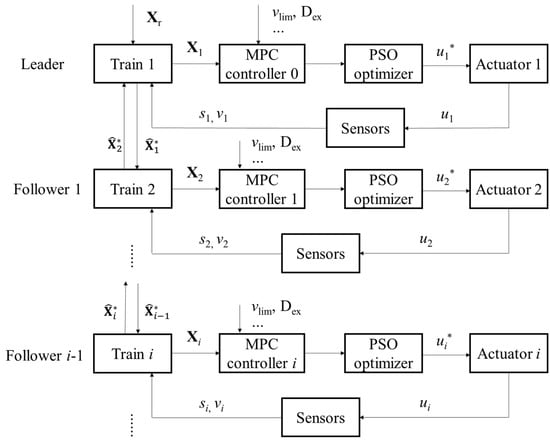
Figure 3.
The PSO-based DMPC framework, where the superscript sign ‘*’ represents the actual value of the parameter.
4. Result
The simulation experiments consist of two parts: validation of algorithm effectiveness and analysis of the adaptive mechanism. The first part of the experiments verifies that the proposed method can ensure the stable operation of the VCTS from multiple perspectives, including different initial tracking speeds, speed and distance differences between adjacent trains, tracking speed, and position errors. The second part analyzes the performance of Algorithm 1, comparing the ability of controllers with and without the ADM to handle uncertainties of the train dynamic model.
4.1. Experiment Setup
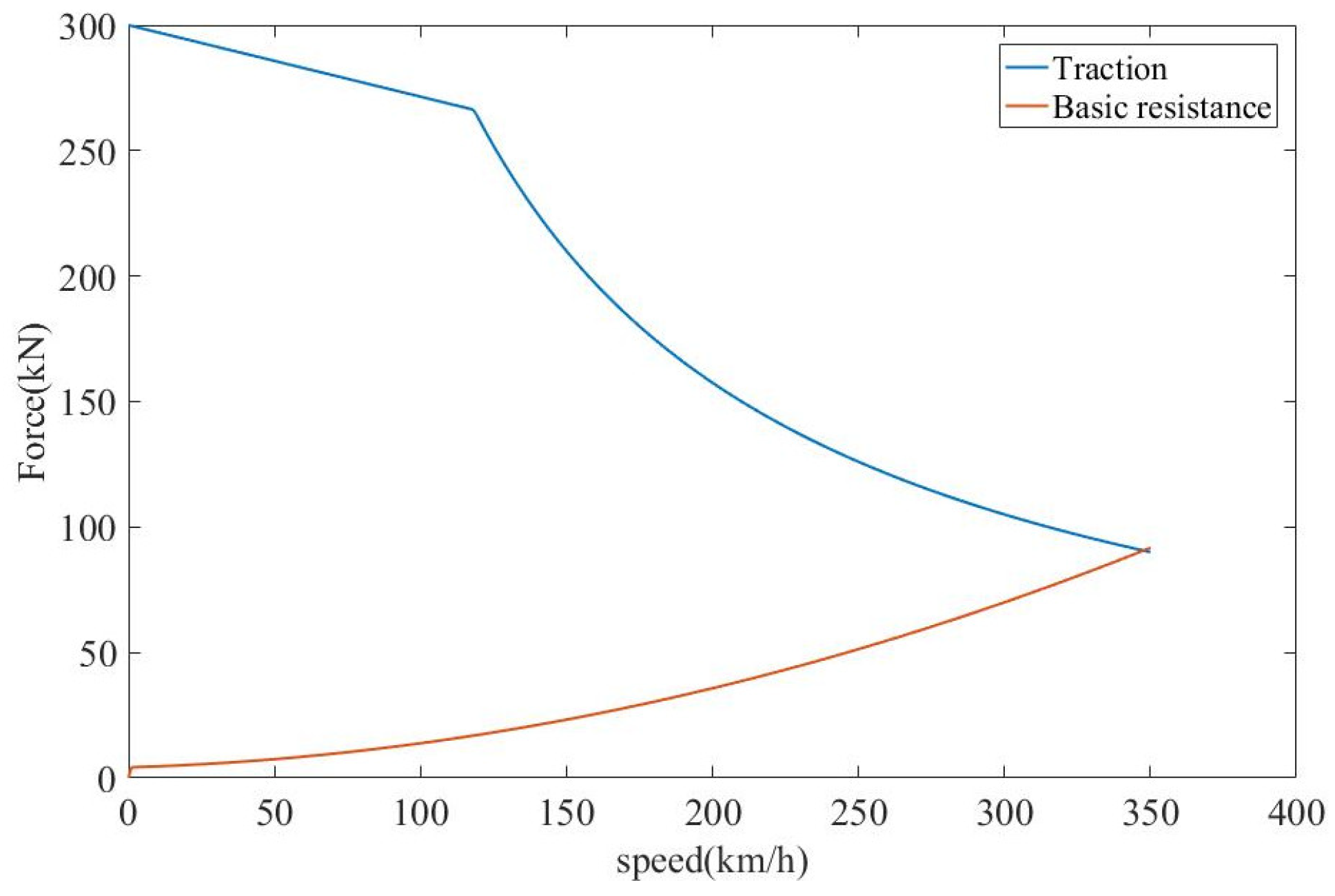
The length of the railway line in the simulation is set as 80 km and the gradient of the line is shown in Table 1. The VCTS consists of four trains, e.g., one leader train and three follower trains. The reference trajectory is a cruising profile along the line at a speed of 288 km/h, which the leader train needs to track accurately. Four CRH-3 trains are used in the simulation. The traction characteristic curve and the basic resistance profile of the CRH-3 train are shown in Figure 4. The parameters of the CRH-3 train and the proposed controller are listed in Table 2 and Table 3, respectively. Experiments are conducted on a PC (2.6 GHz processor speed and 4 GB memory size) with the OS of Windows 11. The simulation software is Matlab2016b.

Table 1.
The gradient of the simulation line.
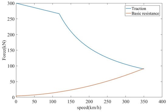
Figure 4.
The traction characteristic curve and the basic resistance profile of the CRH-3 train.
Table 2.
Parameters of the CRH-3 train.
Table 3.
Parameters of the proposed controller.
4.2. Method Effectiveness Validation
The effectiveness of the proposed algorithm is analyzed from two aspects, including tracking performance and convergence performance.
First, we introduce the simulation parameters of this experiment. The speeds of the leader train and the three follower trains are set to 288 km/h, 284.4 km/h, 280.8 km/h, and 277.2 km/h, respectively. The tracking distances between the leader train and follower train 1, between follower train 1 and follower train 2, and between follower train 2 and follower train 3 are all set to 350 m. The initial train basic resistance is selected according to Table 2 and Equation (2). Because of the exterior disturbances, we set the actual train basic resistance as , where .
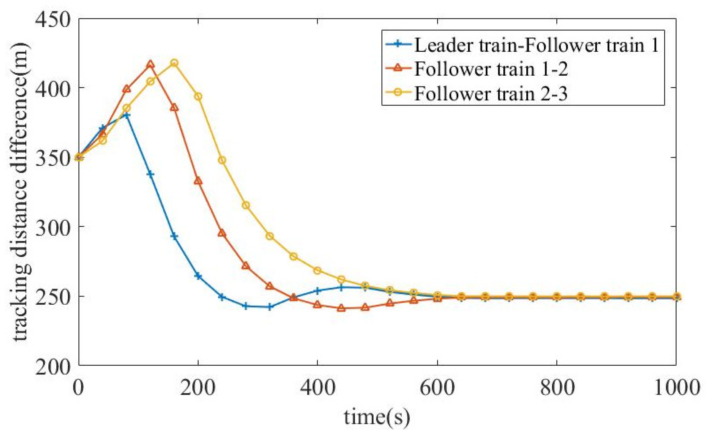
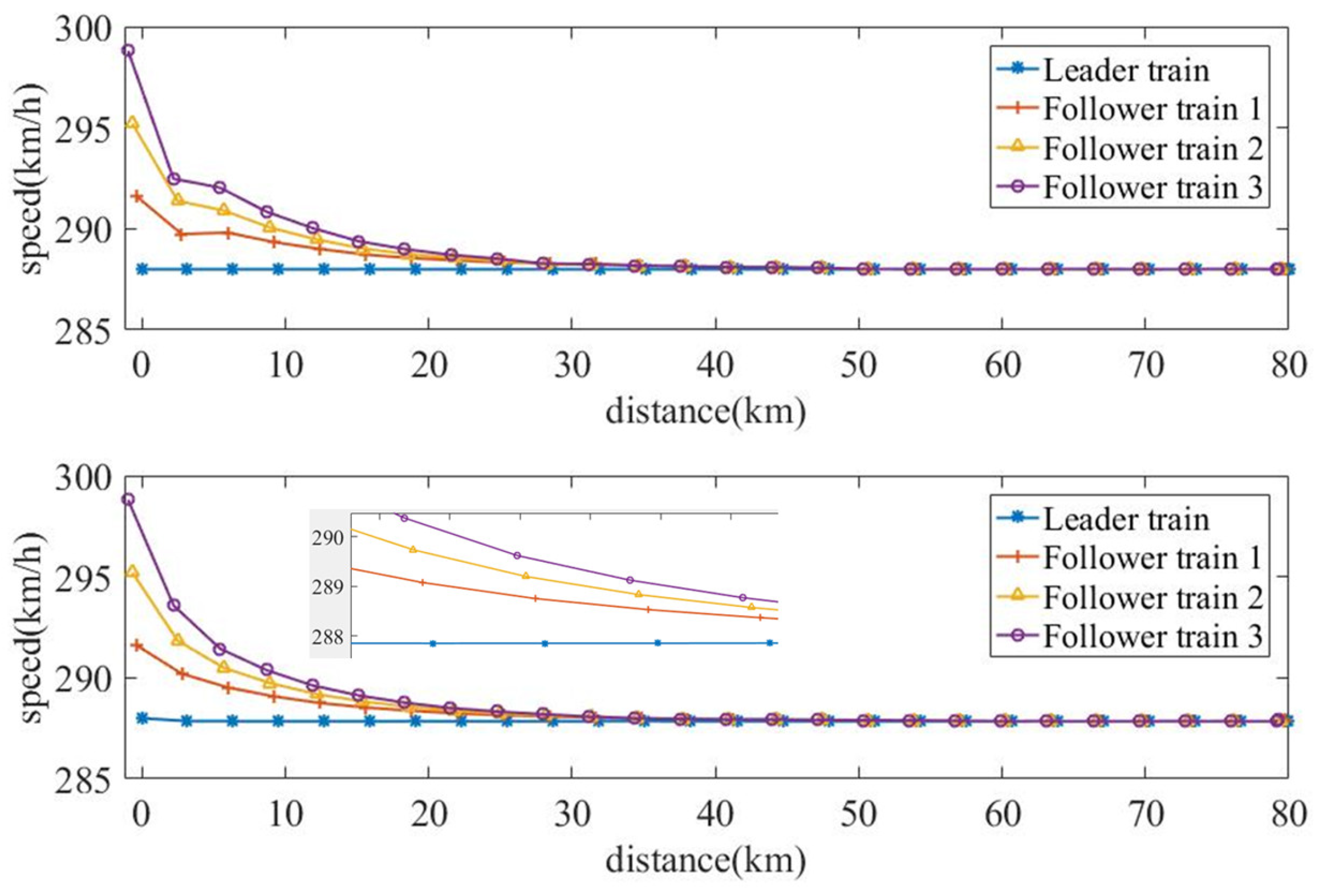
The tracking performance of trains in the VCTS at different initial speeds is shown in Figure 5, Figure 6 and Figure 7. The leader train precisely tracks the expected profile at a constant speed of 288 km/h. Due to the initial tracking speed and the distance between adjacent trains, the control strategy for the three follower trains first requires acceleration. This causes the tracking distance between neighboring trains to increase further. When the follower trains reach 292 km/h, 296 km/h, and 298 km/h, respectively, they begin to decelerate to balance the speed and distance tracking performance.
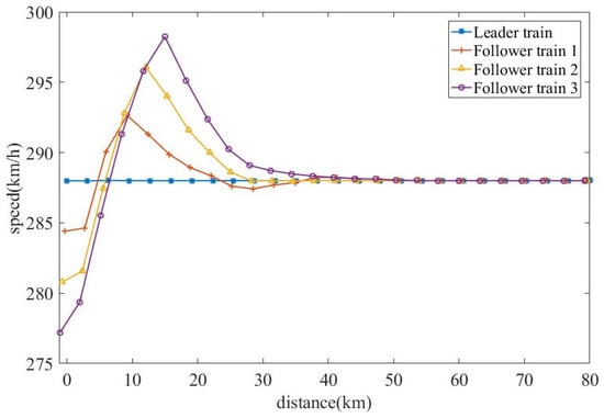
Figure 5.
The speed profiles of trains in the VCTS at different initial speeds.
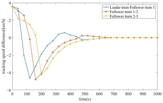
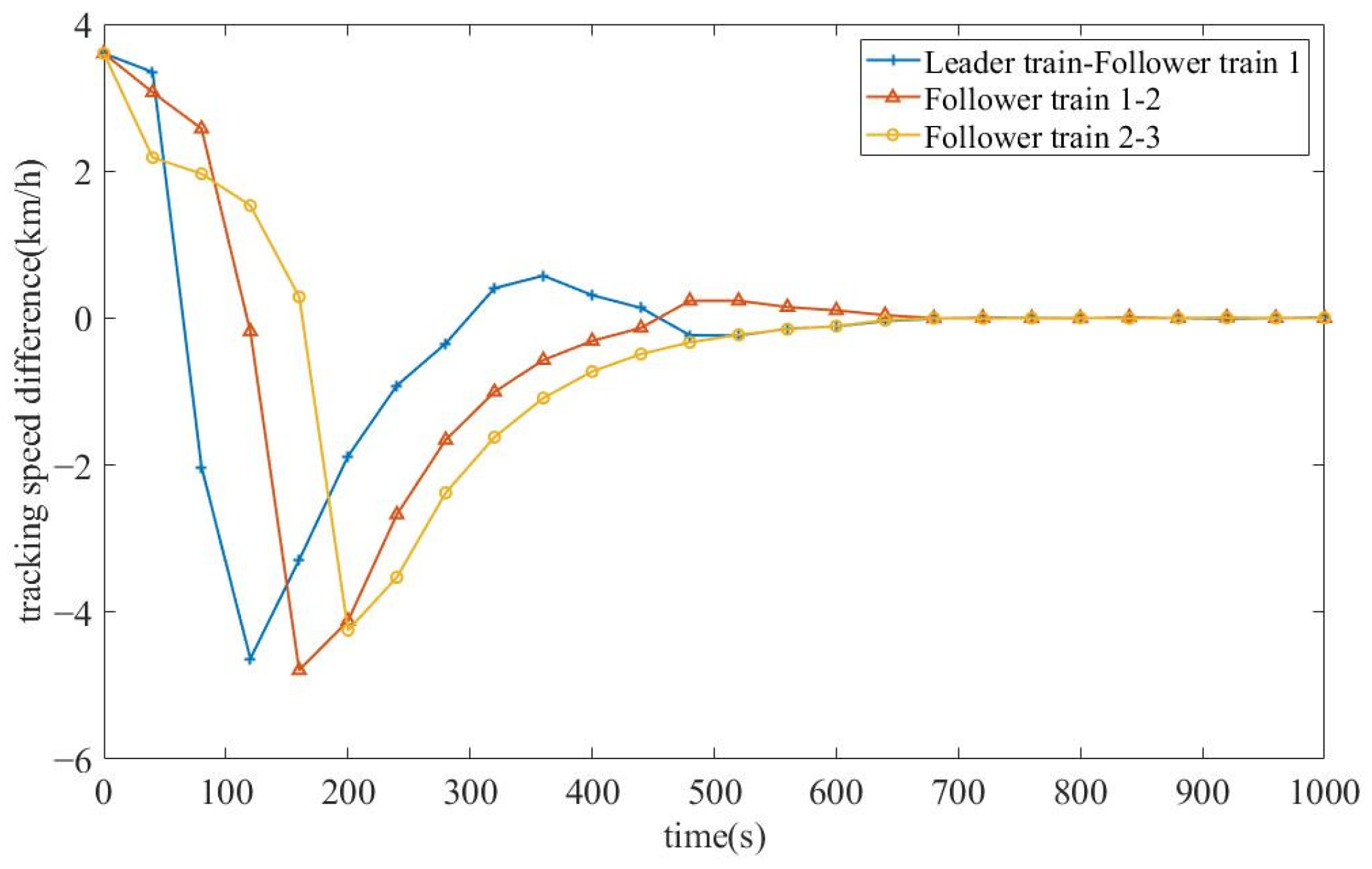
Figure 6.
The tracking speed difference profiles of each neighboring train.
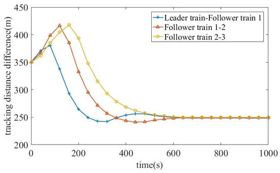
Figure 7.
The tracking distance difference profiles of each neighboring train.
Since follower trains 1 and 2 have bidirectional T2T communication, their tracking speeds fluctuate around the expected cruising speed. In contrast, follower train 3 only receives state information and predicted state information within a horizon from follower train 2, resulting in larger variations in tracking speed and distance that require regulation. Consequently, the speed profile of follower train 3 gradually converges to the desired value. Finally, the VCTS reaches stable operation at 51 km.
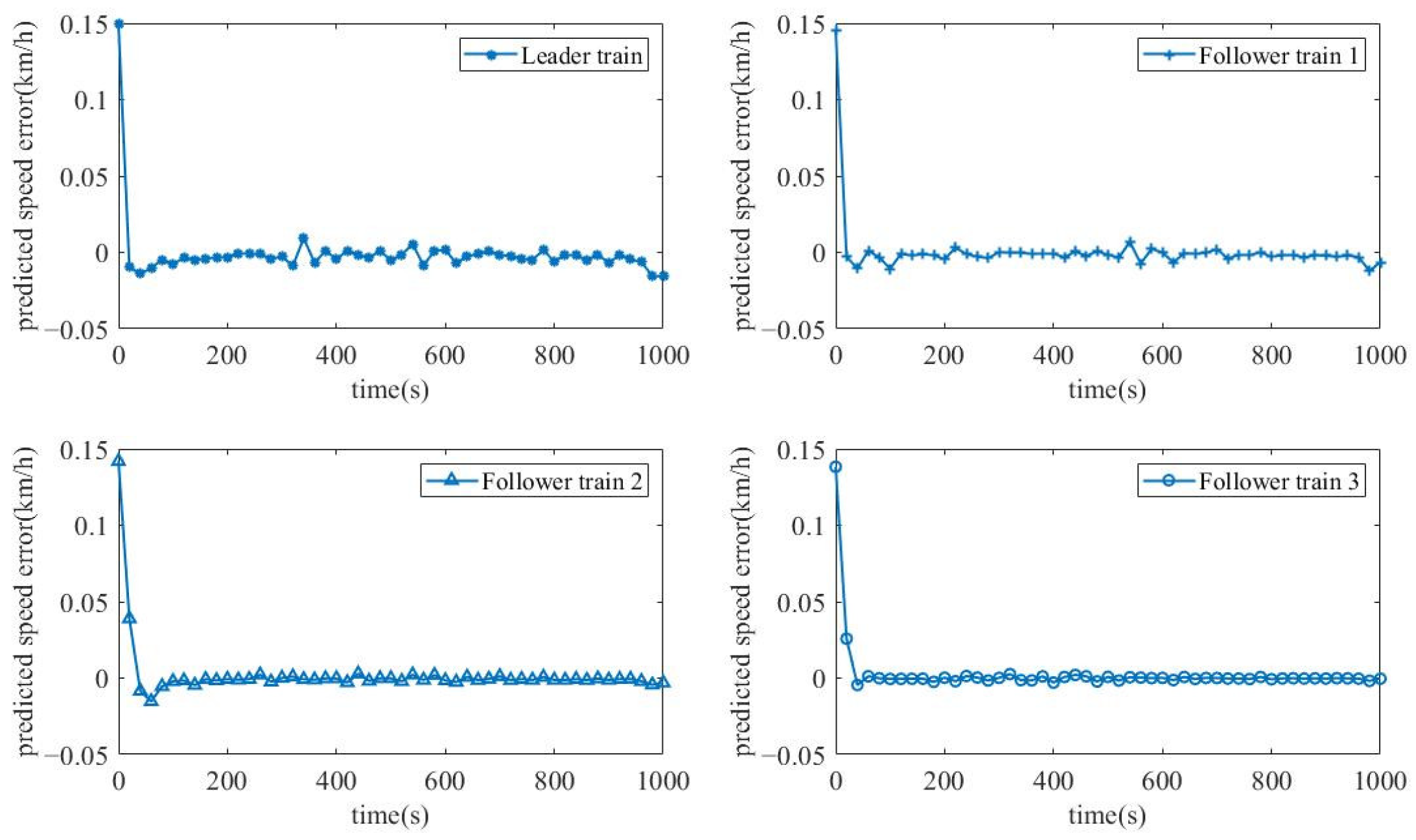
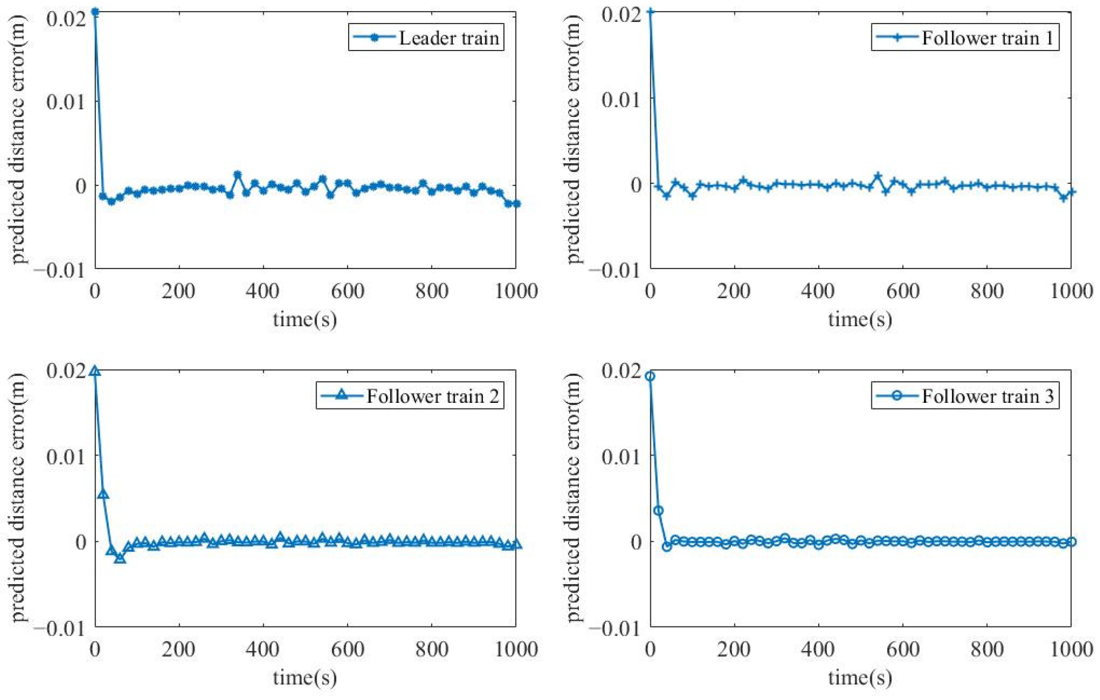
Figure 8 and Figure 9 show the predicted speed error and distance error for each train in the VCTS using the proposed algorithm. This experiment aims to verify whether the designed adaptive mechanism is able to adjust the train model to the real value. In actuality, it is difficult to calculate every single value in the train model matrix . Therefore, we choose to estimate the systematic model as a whole instead of conducting parameter identification. Due to the influence of train model bias, the initial predicted speed error is 0.15 km/h, and the initial predicted distance error is 0.02 m. The adaptive mechanism can adjust according to the system tracking error, meaning that it will optimize the train model parameters to match the real one. After approximately 80 s, the predicted speed and distance errors converge to zero.
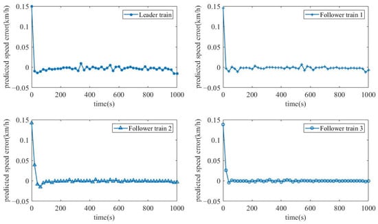
Figure 8.
The predicted speed error profiles of trains in the VCTS.
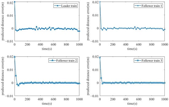
Figure 9.
The predicted distance error profiles of trains in the VCTS.
Additionally, we use the rate of change in acceleration, called jerk, to represent the train control comfort index. From the simulation results, the maximum jerk values are 0.205 m/s3 for the leader train, 0.208 m/s3 for follower train 1, and 0.210 m/s3 for follower trains 2 and 3. The average values of jerk for the trains in the VCTS are 0.00004 m/s3, 0.00015 m/s3, 0.00015 m/s3, and 0.00006 m/s3, respectively.
4.3. Adaptive Mechanism Analysis
This experiment aims to compare the tracking performance and train state prediction performance with and without the adaptive mechanism (ADM) under multiple disturbance conditions.
The simulation parameters are set as follows. The speed of the leader train is set to 288 km/h, while three follower trains operate at 291.6 km/h, 295.2 km/h, and 298.8 km/h, respectively. The tracking distances are configured as follows: 350 m between the leader train and follower train 1, and 300 m each between follower trains 1 and 2 and between follower trains 2 and 3. The actual train basic resistance is set as , where and . Additionally, we consider the input perturbation of the catenary and traction system, and follows the Gaussian distribution, .
Figure 10 shows the tracking performance comparison of trains in the VCTS with and without the ADM. We can observe that the trends of the profiles in Figure 10 differs from those in Figure 5. This is because the speed of follower trains 1–3 exceeds the desired cruising speed, even though the initial tracking distance remains constant at around 300 m. Thus, the controller in this simulation adjusts the control input to balance tracking speed and distance directly. From Figure 10, we see that both groups of profiles converge to a cruising speed, though the final speeds differ. The VCTS with the ADM converges to 288 km/h, while the one without the ADM converges to 287.8 km/h. This discrepancy occurs because the MPC controller, based on the nominal train model, cannot fully eliminate the bias relative to the real model.
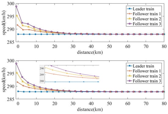
Figure 10.
The speed profiles of the trains in the VCTS with and without the ADM.
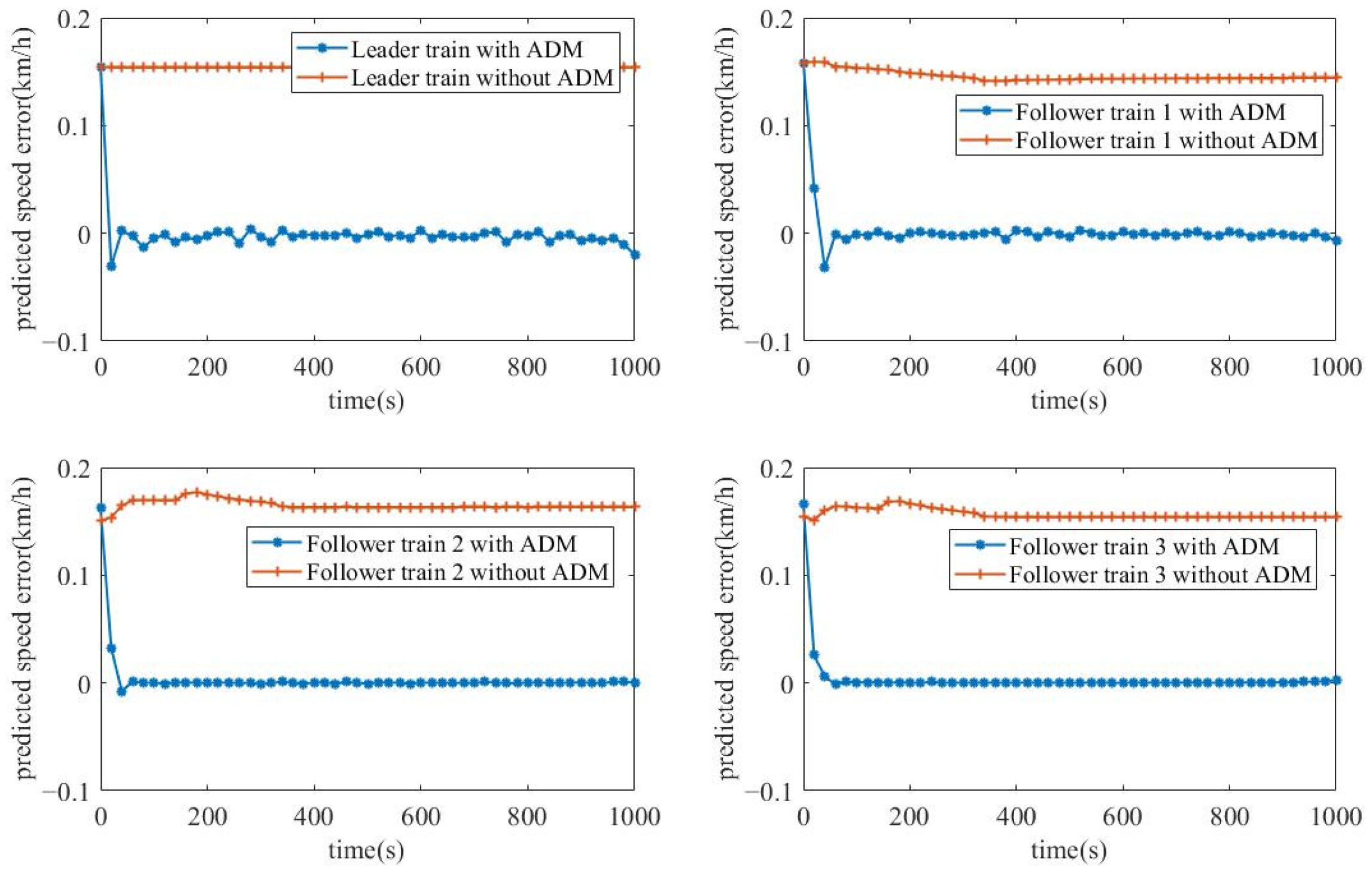
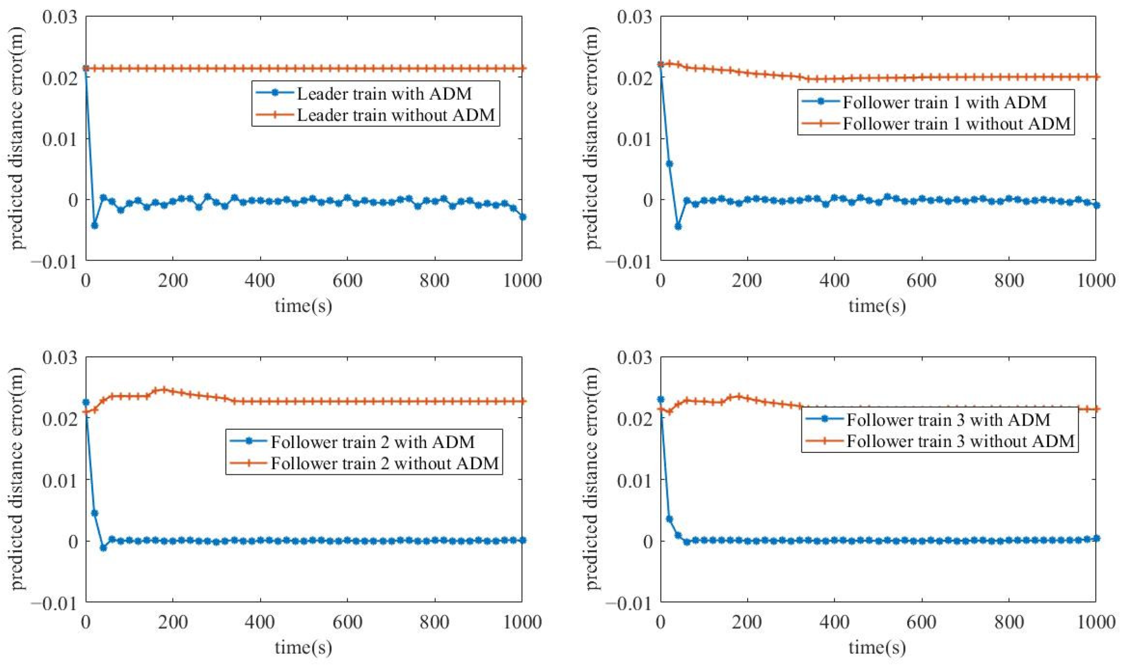
Figure 11 and Figure 12 illustrate the predicted speed and distance error profiles of trains in the VCTS with and without the ADM. We observe that the predicted state values of the controller with the ADM converge to zero after 40 s, indicating that the predicted train model has aligned with the actual model. In contrast, the predicted state values of the controller without the ADM exhibit fluctuations until 400 s, as the VCTS had not yet reached a stable condition.

Figure 11.
The predicted speed error profiles of trains in the VCTS with and without the ADM.
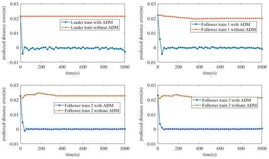
Figure 12.
The predicted distance error profiles of trains in the VCTS with and without the ADM.
Within the DMPC optimization horizon, the controller consistently uses the nominal model for planning. Although DMPC inherently provides robustness against disturbances, a persistent error exists between the nominal model and the actual model. As a result, the predicted speed error and distance error converge to 0.17 km/h and 0.021 m, respectively.
To evaluate the passenger comfort under multi-disturbance conditions, we analyze the jerk performance of the proposed algorithm. The maximum jerk of the leader train is 0.205 m/s3, that of follower train 1 is 0.203 m/s3, and that of follower trains 2 and 3 is 0.202 m/s3. The average values of jerk for trains in the VCTS are 0.00004 m/s3, 0.00017 m/s3, 0.00017 m/s3, and 0.00018 m/s3, respectively.
Since MPC is an online controller, the calculation time of each horizon is recorded accordingly. The average computation times for the two experiments were 50.38 ms and 50.21 ms, respectively. Given that the control period of actual ATO actuator in China is 200 ms, the proposed algorithm satisfies real-time requirements for the operation of the VCTS.
5. Conclusions
This paper presents a DMPC approach for the control of VCTS which incorporates uncertainties in basic resistance and control inputs, utilizing an ADM to mitigate errors caused by external disturbances. A multi-objective optimization model was established, considering position error, speed error, and ride comfort, while enforcing constraints such as actuator saturation, speed limits, and safe tracking distance. The PSO algorithm was employed to solve the non-convex optimization problem globally, ensuring robust and efficient control.
Simulation experiments demonstrated the effectiveness of the proposed method in achieving stable operation of VCTS under various initial conditions. The performance of the adaptive mechanism was compared with that of a non-adaptive controller, revealing that the ADM effectively handled uncertainties in the train dynamics model and achieved the reduction of tracking errors while improving ride comfort.
In conclusion, the proposed DMPC approach, combined with ADM and PSO optimization, offers a promising solution for the control of VCTS. Future work could explore the integration of additional real-world constraints and further validation in diverse operational environments to enhance the practical applicability of the proposed method.
Author Contributions
Conceptualization, Z.H. (Zhiyu He), Z.H. (Zhuopu Hou) and N.X.; methodology, Z.H. (Zhiyu He), Z.H. (Zhuopu Hou) and D.L.; software, Z.H. (Zhiyu He); investigation, Z.H. (Zhuopu Hou); writing—original draft preparation, Z.H. (Zhuopu Hou) and Z.H. (Zhiyu He); writing—review and editing, N.X., D.L. and M.Z.; supervision, N.X., D.L. and M.Z. All authors have read and agreed to the published version of the manuscript.
Funding
This research was funded by the National Nature Science Foundation of China (grant number 12473072), the Science and Technology Research Project of China Railway (grant number L2024G004), and the Major Project of China Academy of Railway Sciences Co., Ltd. (grant number 2023YJ312).
Data Availability Statement
The original contributions presented in this study are included in the article. Further inquiries can be directed to the corresponding author.
Conflicts of Interest
Authors Zhiyu He, Zhuopu Hou, Ning Xu, Dechao Liu were employed by the China Academy of Railway Sciences Corporation Limited. The remaining authors declare that the research was conducted in the absence of any commercial or financial relationships that could be construed as a potential conflict of interest.
References
- Dong, H.; Ning, B.; Cai, B.; Hou, Z. Automatic train control system development and simulation for high-speed railways. IEEE Circuits Syst. Mag. 2010, 10, 6–18. [Google Scholar] [CrossRef]
- Ning, B.; Tang, T.; Qiu, K.; Gao, C. CBTC (Communication Based Train Control): System and development. WIT Transactions on State of the art in Science and Engineering. WIT Trans. State Art Sci. Eng. 2010, 46, 37–44. [Google Scholar]
- Mo, Z. Prospect on Technical Development of Intelligent Railway Train Control System. Railw. Signal. Commun. 2022, 58, 1–7. [Google Scholar]
- Ning, B. Absolute braking and relative distance braking—Train operation control modes in moving block systems. WIT Trans. Built Environ. 1998, 34, 991–1001. [Google Scholar]
- Bock, U.; Varchmin, J.U. Enhancement of the Occupancy of Railroads Using Virtually Coupled Train Formations. In Proceedings of the World Congress on Railway Research (WCRR), Tokyo, Japan, 16–20 November 1999. [Google Scholar]
- Xun, J.; Li, Y.; Liu, R.; Li, R.; Liu, Y. A Survey on Control Methods for Virtual Coupling in Railway Operation. IEEE Open J. Intell. Transp. Syst. 2022, 3, 838–855. [Google Scholar] [CrossRef]
- Wu, Q.; Ge, X.; Han, Q.L.; Liu, Y. Railway Virtual Coupling: A Survey of Emerging Control Techniques. IEEE Trans. Intell. Veh. 2023, 8, 3239–3255. [Google Scholar] [CrossRef]
- Felez, J.; Vaquero-Serrano, M.A. Virtual Coupling in Railways: A Comprehensive Review. Machines 2023, 11, 521. [Google Scholar] [CrossRef]
- Su, H.; Chai, M.; Chen, L.; Lv, J. Deep learning-based model predictive control for virtual coupling railways operation. In Proceedings of the 2021 IEEE International Intelligent Transportation Systems Conference (ITSC), Indianapolis, IN, USA, 19–22 September 2021; pp. 3490–3495. [Google Scholar]
- Tang, H.; Wang, Q.; Feng, X. Robust stochastic control for high-speed trains with nonlinearity, parametric uncertainty, and multiple time-varying delays. IEEE Trans. Intell. Transp. Syst. 2017, 19, 1027–1037. [Google Scholar] [CrossRef]
- Ding, Y.; Lyu, J.; Liu, C.; Gao, J.; Lyu, J. Research on Train Collaborative Control Method for Urban Rail Transit Based on Distributed Model Predictive Control. Railw. Signal. Commun. 2024, 60, 11–19. [Google Scholar]
- Felez, J.; Kim, Y.; Borrelli, F. A model predictive control approach for virtual coupling in railways. IEEE Trans. Intell. Transp. Syst. 2019, 20, 2728–2739. [Google Scholar] [CrossRef]
- Wang, P.; Zhu, Y.; Zhu, W. Robust cooperative train trajectory optimization with stochastic delays under virtual coupling. IET Intell. Transp. Syst. 2023, 17, 1415–1433. [Google Scholar] [CrossRef]
- Park, J.; Lee, B.-H.; Eun, Y. Virtual coupling of railway vehicles: Gap reference for merge and separation, robust control, and position measurement. IEEE Trans. Intell. Transp. Syst. 2020, 23, 1085–1096. [Google Scholar] [CrossRef]
- Muniandi, G. Blockchain-enabled virtual coupling of automatic train operation fitted mainline trains for railway traffic conflict control. IET Intell. Transp. Syst. 2020, 14, 611–619. [Google Scholar] [CrossRef]
- Mayne, D.Q.; Rawlings, J.B.; Rao, C.V.; Scokaert, P.O.M. Constrained model predictive control: Stability and optimality. Automatica 2000, 36, 789–814. [Google Scholar] [CrossRef]
- Felez, J.; Vaquero-Serrano, M.A.; de Dios Sanz, J. A Robust Model Predictive Control for Virtual Coupling in Train Sets. Actuators 2022, 11, 372. [Google Scholar] [CrossRef]
- Vaquero-Serrano, M.A.; Felez, J. A decentralized robust control approach for virtually coupled train sets. Comput.-Aided Civ. Infrastruct. Eng. 2023, 38, 1896–1915. [Google Scholar] [CrossRef]
- Liu, Y.; Liu, R.; Wei, C.; Xun, J.; Tang, J. Distributed Model Predictive Control Strategy for Constrained High-Speed Virtually Coupled Train Set. IEEE Trans. Veh. Technol. 2022, 71, 171–183. [Google Scholar] [CrossRef]
- Liu, X.; Dabiri, A.; Wang, Y.; Xun, J.; De Schutter, B. Distributed Model Predictive Control for Virtually Coupled Heterogeneous Trains: Comparison and Assessment. IEEE Trans. Intell. Transp. Syst. 2024, 25, 20753–20766. [Google Scholar] [CrossRef]
- Luo, X.; Tang, T.; Liu, H.; Zhang, L.; Li, K. An Adaptive Model Predictive Control System for Virtual Coupling in Metros. Actuators 2021, 10, 178. [Google Scholar] [CrossRef]
- Luo, X.; Tang, T.; Yin, J.; Liu, H. A robust MPC approach with controller tuning for close following operation of virtually coupled train set. Transp. Res. Part C Emerg. Technol. 2023, 151, 104116. [Google Scholar] [CrossRef]
- Bai, W.; Lin, Z.; Dong, H.R.; Ning, B. Distributed cooperative cruise control of multiple high-speed trains under a state-dependent information transmission topology. IEEE Trans. Intell. Transp. Syst. 2019, 20, 2750–2763. [Google Scholar] [CrossRef]
- Diwan, S.P.; Deshpande, S.S. Fast nonlinear model predictive controller using parallel PSO based on divide and conquer approach. Int. J. Control 2022, 96, 2230–2239. [Google Scholar] [CrossRef]
- Hong, S.H.; Ou, J.; Wang, Y. Physics-guided neural network and GPU-accelerated nonlinear model predictive control for quadcopter. Neural Comput. Appl. 2022, 35, 393–413. [Google Scholar] [CrossRef]
- Fan, W.; Hu, Z.; Veerasamy, V. PSO-Based Model Predictive Control for Load Frequency Regulation with Wind Turbines. Energies 2022, 15, 8219. [Google Scholar] [CrossRef]


Disclaimer/Publisher’s Note: The statements, opinions and data contained in all publications are solely those of the individual author(s) and contributor(s) and not of MDPI and/or the editor(s). MDPI and/or the editor(s) disclaim responsibility for any injury to people or property resulting from any ideas, methods, instructions or products referred to in the content. |
© 2025 by the authors. Licensee MDPI, Basel, Switzerland. This article is an open access article distributed under the terms and conditions of the Creative Commons Attribution (CC BY) license (https://creativecommons.org/licenses/by/4.0/).