Enhanced CO₂ Emissions Prediction Using Temporal Fusion Transformer Optimized by Football Optimization Algorithm

Abstract

The accurate prediction of carbon dioxide (CO₂) emissions from light-duty vehicles is critical for mitigating environmental impacts and enhancing regulatory compliance in the automotive industry. However, challenges such as high-dimensional feature spaces, feature redundancy, and hyperparameter sensitivity limit the efficiency of machine learning (ML) models in CO₂ emissions forecasting. This study systematically investigates the efficacy of ML models for CO₂ emissions prediction using the Fuel Consumption Ratings 2023 dataset, with a particular focus on optimizing feature selection and hyperparameter tuning through metaheuristic techniques. The performance of various ML models, including the Temporal Fusion Transformer (TFT), is evaluated before and after optimization. Initially, the TFT model achieved a root mean squared error (RMSE) of 0.082723421 in the baseline scenario. Feature selection using the Football Optimization Algorithm (FbOA) significantly improved its performance, reducing the RMSE to 0.018798774. Further enhancement through metaheuristic optimization using FbOA resulted in an exceptionally low RMSE of 0.000923, demonstrating substantial gains in predictive accuracy. The findings underscore the impact of metaheuristic-driven feature selection and hyperparameter tuning in optimizing ML models for environmental sustainability applications. This work provides a framework for integrating advanced ML methodologies with optimization techniques, offering policymakers and automotive manufacturers a robust tool for assessing and reducing vehicle emissions.

1. Introduction

The unprecedented rate of climate change resulting from increasing concentrations of greenhouse gases in the atmosphere has led to urgent calls for policy and technological intervention [1]. However, the carbon dioxide (CO₂) emissions from the transportation sector are one of the highest GHG contributors among all sectors, contributing substantially to global emissions. In particular, a reasonable fraction of fossil fuel consumption and carbon emissions relates to light-duty vehicles, which most people and firms use as their means of personal and commercial transportation, respectively, worldwide. As towns and cities grow, personal and commercial transport is becoming more necessary, and the curtailment of vehicular emissions is an absolute necessity [2].

Regulations for minimizing vehicle emissions have been enforced by making vehicle efficiency standards and encouraging the usage of cleaner energy sources worldwide by governments and environmental agencies. Among such regulations are CAFE (corporate average fuel economy) standards, emissions trading schemes, and tax incentives for lower emissions vehicles [3]. Simultaneously, auto manufacturers must develop energy-efficient vehicles with the lowest possible carbon footprint. Designing such vehicles demands in-depth knowledge about the emission patterns and capable predictive models that are able to predict emissions accurately using vehicle specifications [4].

CO₂ emissions prediction is a central problem for manufacturers when designing more fuel-efficient vehicles and has critical implications in policymaking and environmental planning. Policymakers, in turn, must establish better regulations for vehicle emissions control, enabling consumers to choose the vehicle they want based on the more knowledgeable decisions. Since emissions often involve many interacting factors, including vehicle engine size, type of transmission, type of fuel, and vehicle aerodynamics, devoping reliable prediction models is difficult [5]. The complex nonlinear relationships in vehicular attributes make it difficult for traditional emissions estimation models primarily based on physical and statistical regression techniques. Most of these methods are based on predefined assumptions, which generalize poorly across different vehicle types and driving conditions, and therefore, they do not have tremendous practical applicability [6].

Therefore, machine learning (ML) techniques present a revolutionary way of predicting emissions by using data-driven methodologies to learn the complex relationships in the massive datasets that are adapted. However, ML models have been shown to perform significantly better than conventional models in capturing intricate patterns on high dimensional spaces and, hence, outperform them in prediction accuracy [7]. Advances in the field of ML, most notably in the realm of deep learning and ensemble modeling, have allowed these models to outperform other such models in a state-of-the-art way in various applications, including emissions forecasting. ML algorithms differ from traditional methods in that they do not require any assumptions regarding the feature dependencies; instead, they complete the learning from the data themselves and are naturally flexible, with the ability to accommodate a wide range of vehicle specifications. In addition, real-world driving patterns and contextual information can be integrated into ML-based emissions modeling to make it predictive, robust, and reliable [8].

While there already exist ML-based approaches for CO₂ emissions prediction, there remain several fundamental challenges that need to be addressed for accurate and efficient forecasting. The primary challenge stems from vehicular datasets being of high dimensionality [9]. For example, emissions data will likely contain several features, including vehicle engine characteristics, fuel consumption variables, aerodynamic properties, etc. A large number of variables increases computational complexity, which necessitates the use of advanced feature selection algorithms to select only a few essential variables that are most relevant and to relegate those that are not similar to irrelevant or redundant attributes. Similarly, the curse of dimensionality can also arise from long geodesic distances in high dimensional spaces due to the sparsity of data in the high dimensional space [10].

Feature redundancy is another big issue—this relates to multiple features among vehicle attributes showing strong correlations. For example, metric fuel consumption measured out through city, highway, and combined driving conditions can be highly collinear, providing additional redundant information, which sometimes negatively influences the model generalization [11]. Specifically, redundant features add noise to the learning problem and confuse the model, increasing its complexity and impeding the ability to interpret the underlying factors that influence emissions. In the case of graphs, feature selection techniques are required to identify and keep only the most informative variables so that the model is not prevented from becoming computationally efficient and interpretable [12].

One of the additional challenges of ML-based emissions prediction is the sensitivity of hyperparameters. The ability of ML models to perform well is hugely dependent on hyperparameter tuning, which entails selecting the best values for parameters such as the learning rate, regularization coefficient, and especially model depth [13]. Suboptimal hyperparameter configuration results in overfitting, where the model learns the noise over a meaningful pattern, or underfitting, where the model does not fit the underlying data structure well. Due to the ample search space of possible hyperparameter values, manual tuning is generally infeasible; thus, various robust optimization techniques are used in order to automate and improve the process of selecting hyperparameters [13].

The difficulties in emissions prediction tasks are further generalization and overfitting. ML models are very accurate if they can predict the training data; however, their performance worsens when deployed onto new and unseen vehicle data. A model that overfits relates to one that excessively adapts to the training data by memorizing certain noises and idiosyncrasies rather than learnable patterns [14]. To address the issue, some network methods such as cross-validation, dropout regularization, and feature selection are used to keep the complexity of the model balanced and to maintain the generalization performance. In addition, black box models generally need to remain interpretable and explainable, although, particularly in the context of regulations or policymaking, black box models may not be readily adopted [15].

This study aims to design and validate the performance of ML-based approaches that predict CO₂ emissions in light-duty vehicles from the Fuel Consumption Ratings 2023 dataset. In this research, many ML models are evaluated systematically concerning their success in emissions forecasting, overcoming the main challenges of feature selection, dimensionality reduction, and hyperparameter optimization [16]. This study will determine the most effective prediction framework with the necessary accuracy and computational efficiency with state-of-the-art ML techniques [17].

This work views feature selection and hyperparameter tuning as methods to enhance emissions prediction accuracy using metaheuristic optimization techniques as a core focus of this work [18]. The reduction in dataset dimensionality with the retention of the most relevant attributes is achieved by feature selection. The goal is also to improve the models’ interpretability and computational performance. At the same time, we ensure that ML models are trained in optimal conditions through hyperparameter optimization to avoid underfitting and overfitting [19].

This research also intends to establish a computationally efficient and scalable framework to generate an emissions model. One study decreased the complexity of ML models and eased the feature selection and hyperparameter tuning process, producing a robust methodology that can be further expanded into more general environmental modeling issues [20]. This research has value not only in the context of academia but also as a means to discover valuable insights for use in governmental compliance monitoring, eco-friendly vehicle design, and the integration of intelligence for operational control in the intelligent transportation system.

The study helps improve the development of intelligent decision support systems that will benefit automotive manufacturers, policymakers, and even consumers. The aim is to create a sound and data-driven way of approaching the trade-off analysis and mitigation of vehicular CO₂ emissions with the ultimate goal of contributing to a more sustainable transportation sector.

2. Literature Review

Climate change and global warming are very pressing environmental concerns, mainly attributed to the emission of greenhouse gases (GHGs), particularly carbon dioxide (CO₂). Due to its high output of CO₂ emissions, changing the transport sector so that based on efficient monitoring and predictive modeling techniques is a must. There has been a rise in the application of machine learning (ML) and optimization algorithms to predict CO₂ emissions and which of its factors are key. The present work explores methodologies used in recent research for CO₂ emissions estimation and analysis using ML and metaheuristic techniques.

A couple of studies have proposed innovative ways of predicting CO₂ emissions through the use of an RNN-based Long Short Term Memory (LSTM) approach from On-Board Diagnostics (OBD-II) data [21]. This method offers an easy means of emissions monitoring in real-time. Using the same type of predictive emission monitoring system, ref. [22] used their predictive emission monitoring system with feature engineering and a hyperparameter tuning of workflows, achieving better accuracy with Deep Forest Regression (DFR).

In their study, ref. [23] propose a UPGO updated grey multivariable convolution model for provincial carbon emissions forecasting in China—the model with an MAPE less than 4% obtained good prediction accuracy for sample periods. Additionally, ref. [24] exploited a BPNN in conjunction with PSO to further analyze the CO₂ emission prediction and more effectively determine energy consumption management policies.

An interpretable multi-stage forecasting framework coupled with SHAP-based explanations was used in [25] for predicting the CO₂ emissions of the UK transportation sector, thereby making another important contribution. As stated in their findings, road carbon intensity was the most important influencing factor.

One study, ref. [26], combined a multi-objective mathematical model with ML algorithms to predict energy demand and CO₂ emissions in Canada’s transportation sector. Sensitivity analyses were run to indicate how varying energy sources impacted the emissions trend. As in [27], the MRFO-ELM hybrid model was proposed to forecast China’s transport CO₂ emissions and it was found that vehicle electrification is important for emission trends.

Ref. [28] used a novel Random Forest (RF) approach to predict diesel engine emissions with applied SHAP-based interpretability techniques for emissions from internal combustion engines. For most engine parameters, R² values above 0.98 were achieved for the results. Additionally, ref. [29] also used an optimized wavelet transform Hausdorff multivariate grey model (OWTHGM(1, N)) for forecasting CO₂ emission in Cameroon with an MAPE of 1.27%.

Ref. [30] has adopted the Marine Predators Algorithm (MPA)- and Lightning Search Algorithm (LSA)-based metaheuristic algorithms to produce greenhouse gas trajectories in India from a global perspective. The results project that CO₂ emissions would increase by 2.5 to 2.87 times by 2050. In addition, ref. [31] enhanced prediction accuracy by implementing hybrid RF and support vector regression (SVR) models known to result in better prediction, and they optimized them using seven different optimizers. The best-performing model is RF-SMA with an R² of 0.9641.

Lastly, ref. [32] suggested using novel DPRNNs based on NiOA optimization for CO₂ emission forecasting. The results obtained via a statistical analysis of WILCOX and ANOVA tests validated the accuracy of the prediction achieved through their findings.

This literature review encapsulates the recent advancements in the field, highlighting diverse methodologies and their outcomes. The following

Table 1. Detailed summary of literature on CO₂ emissions prediction using ML and optimization algorithms.

Reference	Focus Area	Methodology	Key Findings and Contributions
[21]	Real-time emissions monitoring through OBD-II data	RNN-based LSTM approach, leveraging the capabilities of neural networks for sequential data processing	Demonstrated effective real-time monitoring capabilities, offering a novel approach to vehicular emissions monitoring
[22]	Enhancement of emissions prediction accuracy	Application of Deep Forest Regression (DFR) combined with comprehensive feature engineering and rigorous hyperparameter tuning	Achieved superior accuracy in emissions predictions, illustrating the benefits of deep learning combined with meticulous model tuning
[23]	Forecasting provincial CO2 emissions in China	Updated Grey Multivariable Convolution model (UPGO) that integrates grey system theory with convolutional techniques	Achieved a Mean Absolute Percentage Error (MAPE) of less than 4%, indicating high prediction accuracy over sample periods
[24]	Analysis of CO2 emissions and energy consumption for policymaking support	Integration of Back Propagation Neural Network (BPNN) with Particle Swarm Optimization (PSO) to refine predictions	Enhanced the decision-making process for energy policy by providing accurate predictions and effective policy analysis tools
[25]	Predicting CO2 emissions in the UK transportation sector	Multi-stage forecasting framework coupled with SHAP-based explanations for interpretability	Identified road carbon intensity as the most significant influencing factor on emissions, adding valuable insights for policy interventions
[26]	Predicting energy demand and CO2 emissions in Canada’s transportation sector	Employed a multi-objective mathematical model along with machine learning algorithms, conducting sensitivity analyses	Highlighted how different energy sources impact emissions trends, providing a foundational tool for understanding sector dynamics
[27]	Forecasting transport CO2 emissions in China	MRFO-ELM hybrid model employing Moth-Flame Optimization and Extreme Learning Machine techniques	Pointed out the crucial role of vehicle electrification in managing emissions trends, suggesting strategic focus areas for reducing environmental impact
[28]	Predictive analysis of diesel engine emissions	Utilized a Random Forest approach enhanced with SHAP-based interpretability techniques for deeper insights into variable importance	Achieved exemplary predictive performance with R2 values above 0.98 for most engine parameters, setting a benchmark in emission analytics
[29]	Forecasting CO2 emissions in Cameroon using advanced grey models	Optimized Wavelet Transform Hausdorff Multivariate Grey Model (OWTHGM(1, N)) for accurate forecasting	Exceptionally low MAPE of 1.27%, showcasing the effectiveness of combining wavelet transforms with grey modeling for emissions forecasting
[30]	Projection of greenhouse gas trajectories in India from a global perspective	Application of Marine Predators Algorithm (MPA) and Lightning Search Algorithm (LSA) for scenario analysis	Predicted a substantial increase in CO2 emissions, urging the need for strategic planning and international cooperation in climate policy
[31]	Enhancing prediction models for greenhouse gas emissions using hybrid approaches	Hybrid model combining Random Forest and Support Vector Regression optimized with various algorithms, including the Sine Cosine Algorithm	Achieved an R2 of 0.9641 with the RF-SMA model, demonstrating the strength of hybrid approaches in environmental modeling
[32]	Advanced prediction of CO2 emissions using deep learning and optimization techniques	Novel DPRNNs (Deep Polynomial Recurrent Neural Networks) based on NiOA (Niche-based Invasive Optimization Algorithm)	Statistical analysis via WILCOX and ANOVA tests validated the high accuracy of the predictions, affirming the robustness of the approach

provides a detailed summary of key studies that have leveraged ML and metaheuristic techniques for predicting CO₂ emissions. Each entry in the table elaborates on the focus area, methodologies employed, and significant findings, offering a comprehensive overview of current trends and methodologies in emissions modeling.

In this literature review, significant advances were made in the models developed to predict CO₂ emission based on ML and optimization techniques. LSTM, RF, BPNN, and metaheuristic optimization have all been highly accurate in prediction, where multiple approaches would have been used. Methods such as SHAP also allow integration for increased model transparency. Future research would benefit from real-time tracking systems, a hybrid deep learning approach, and policy-driven optimization strategies to achieve sustainable emission reductions.

The research gap that this paper addresses revolves around the limitations of traditional CO₂ emissions prediction models, which are primarily based on physical and statistical regression techniques. These conventional methods often suffer from poor generalizability across different vehicle types and driving conditions due to their reliance on predefined assumptions. This limitation is critical as it impacts the practical applicability of emissions estimation models in real-world scenarios, where the interactions between numerous vehicular attributes (like engine size, type of transmission, and fuel type) are complex and nonlinear.

In response, this paper introduces a machine learning-based approach utilizing metaheuristic algorithms to enhance feature selection and hyperparameter tuning. This approach aims to overcome the challenges of high-dimensional feature spaces, feature redundancy, and the sensitivity of machine learning models to hyperparameter settings. By leveraging advanced machine learning techniques, the study seeks to develop more robust and accurate predictive models that are not only more adaptable to varying data characteristics but also capable of capturing intricate interactions within the data without the need for explicit assumptions about the underlying relationships.

The integration of machine learning with metaheuristic optimization represents a significant shift towards data-driven methodologies, which are inherently more flexible and suited for managing the complexity and variability inherent in vehicle emissions data. Thus, this paper fills an essential research gap by proposing a framework that potentially increases the accuracy and efficiency of CO₂ emissions predictions, supporting better regulatory compliance and more informed policymaking in the automotive sector.

3. Materials and Methods

3.1. Dataset Description

In the present study, we use the Fuel Consumption Ratings 2023 dataset [33], a distribution of model-specific fuel consumption rating and estimated CO₂ emissions from newly manufactured light-duty vehicles for sale in Canada. This dataset constitutes a much-needed resource for examining the fuel efficiency of the vehicles across manufacturers, drivetrain technology, and engine configurations. Researchers, policymakers, automotive manufacturers, and the industry use it to analyze emissions, assess regulatory compliance, and optimize eco-friendly vehicle design. The dataset is obtained using standardized fuel consumption testing procedures that ensure consistency and comparability on a model evaluation basis. These ratings serve as an essential basis for emissions forecasting and help build predictive models supporting sustainability across the automotive industry.

Estimated emissions reflect the results of controlled laboratory tests with a cycle test methodology. They have embraced this standardized approach of city, highway, and combined driving conditions with the real world, like air conditioning usage, cold start emissions, etc. Establishing the proper operational characteristics of vehicles and considering their applications enables accurate emissions estimation using the dataset, as the emissions values reported for the given CO₂ are not theoretical approximations but rather reflect realistic driving situations. Therefore, the dataset enables robust modeling based on ML by collecting the vehicle’s attributes that play a role in the variability of emissions.

The dataset contains multiple vehicular attributes that describe each vehicle’s engine, transmission system, fuel consumption rates, and emissions profile.

Table 2. Description of features in the Fuel Consumption Ratings 2023 dataset.

Feature	Description	Unit/Value Type
Year	Model year of the vehicle	Year
Make	Manufacturer or brand of the vehicle	Company Name
Model	Specific vehicle model under analysis	Alphanumeric
Vehicle Class	Classification based on weight and size	Category (e.g., Sedan, SUV, Truck)
Engine Size (L)	Displacement volume of the engine	Liters (L)
Cylinders	Number of cylinders in the engine	Integer
Transmission	Type of transmission system	Category (e.g., Automatic, Manual, CVT)
Fuel Type	Type of fuel used	Category (e.g., Gasoline, Diesel, Hybrid)
Fuel Consumption (L/100 km)	Fuel efficiency (liters per 100 km)	L/100 km
Hwy (L/100 km)	Highway fuel consumption	L/100 km
Comb (L/100 km)	Combined fuel consumption across conditions	L/100 km
Comb (mpg)	Combined fuel economy	Miles per gallon (MPG)
CO2 Emissions (g/km)	Amount of CO2 released per kilometer	g/km
CO2 Rating	Ordinal ranking of CO2 emissions performance	Rating Scale
Smog Rating	Classification of vehicle’s smog-forming emissions	Rating Scale

systematically describes the main attributes, their descriptions, and the units of measurement for these features.

The primary aim of this study is to achieve the prediction of the CO₂ emission (g/km), a significant appraisal measure of the vehicle’s environmental impact. The CO₂ emissions are subject to the combined effect of multiple interdependent attributes that vary to include engine size, fuel type, and transmission type; hence, the accurate modeling of CO₂ emissions requires advanced predictive modeling techniques that can handle complex nonlinear relationships.

The dataset consists of 856 samples, with 600 used for training, 128 for validation, and 128 for testing. The dataset is partitioned into three subsets of training, validation, and testing for model evaluation and to prevent overfitting. Our ML models are trained based on the training dataset and validated on the validation set for hyperparameter tuning and performance evaluation. The developed models are evaluated for their generalization by the test dataset, which acts as an independent test set. The partitioning follows a 70%–15%–15% split for training, validation, and testing, respectively. This structure differs from the simplified two-way split shown in Figure 1, which has now been updated to reflect the full three-way partitioning. The partitioning uses an optimal stratified sampling strategy to maintain class balance and data distribution. This stratification ensures that key features such as vehicle class and fuel type are proportionally represented across all subsets. The structure of this partitioning guarantees that the prediction models developed in this study can generalize to new vehicle data, enabling compliance assessment and policy-related decisions in the automotive industry.

3.2. Machine Learning Models

3.2.1. Model Selection Criteria

Machine learning (ML) models for predicting carbon dioxide (CO₂) emissions in light-duty vehicles require selecting ML models with strong predictive capability, robustness against different vehicular attributes, and adaptability to working with different data distributions [34,35]. The selection criteria of the models for this study are primarily based on the predictive accuracy, the computational efficiency, and the interpretability and the generalization performance on unseen vehicle data. Since vehicle attributes like engine size, transmission type, and fuel efficiency are interrelated with a high degree of complexity, the chosen models should be able to capture nonlinear relations and prevent overfitting. They also have to effectively handle high-dimensional feature spaces to make robust, high-dimensional feature space emissions forecasting with a minimal loss of predictive power [36].

Because analyses of thousands of vehicle entries should be performed over scalable and computationally efficient models, the models used in this study must be suitable. Lastly, with regulatory policies and industry standards changing over time, the selected models should show robustness when changing with new vehicle designs and fuel efficiency trends [34,37]. Moreover, an ability to interpret model predictions is also required, as the ntransparency of model emissions allows policymakers, automobile manufacturers, and researchers to know how different vehicle attributes contribute to CO₂ emissions.

Based on these requirements, this work has decided to use a combination of deep learning architectures, automated machine learning (AutoML) frameworks, and statistical time series models. They are very well suited for the problem of emissions forecasting since they can model sequential dependence and high dimensional feature interactions and optimize predictive performance. A description and the key characteristics of each model used in this study are provided in

Table 3. Overview of machine learning models used for CO₂ emissions prediction.

Model	Description	Key Features
TFT	Neural network-based deep learning model with attention mechanisms	Captures short-term and long-term dependencies; interpretable feature importance; handles static and dynamic covariates
PyCaret	Automated ML framework integrating multiple time series forecasting models	Supports ensemble learning, hyperparameter tuning, and automated feature engineering
N-BEATS	Deep learning-based model for univariate and multivariate time series forecasting	Learns trend and seasonality patterns without manual feature engineering; high forecasting accuracy
Prophet	Additive regression-based time series forecasting model	Automatically detects changepoints; incorporates trend and seasonality adjustments
AutoTS	AutoML framework for time series forecasting	Evaluates multiple models (ARIMA, Prophet, ML models) and selects the optimal approach
TBATS	Advanced statistical model for complex seasonality time series forecasting	Handles multiple seasonalities better than classical time series models

[38].

3.2.2. Description of Models

Each of these models has its benefits regarding predictions of emissions. As a deep learning-based sequence modeling framework, attention mechanisms are used to dynamically weight the input features.

The Temporal Fusion Transformer (TFT). This performs very well in the context of learning short-term and long-term dependencies in emissions data [39]. Also, TFT is interpretable in finding out the most influential predictors in a dataset, facilitating feature selection and strategies to reduce emissions. In contrast to conventional deep learning systems that are black boxes, TFT yields explainable predictions, enabling the researcher to determine the auguring order of vehicle parameters relative to emissions.

The PyCaret’s Time Series is a compelling AutoML framework that can simplify the model selection, feature engineering, and hyperparameter tuning aspect of time series. It supports many ML architectures: tree-based such as XGBoost and LightGBM, along with classical forecastings like ARIMA and SARIMA. PyCaret automates the whole ML pipeline and ensures that the best emissions forecasting models are optimally configured without much manual intervention. The ensemble learning capability to combine several models and give its performance predictive stability makes it suitable for emissions modeling.

N-BEATS (Neural Basis Expansion Analysis for Time Series) is a deep learning-based method tailored for forecast applications [40]. However, N-BEATS differs from traditional models that require data to be engineered with explicit features because N-BEATS learns directly from the data what the trend and seasonality patterns are. Flexible architecture enables it to be a better forecaster than conventional models in many real-world applications, thus making it a good candidate for emissions prediction. For forecasting vehicle emissions, N-BEATS is more beneficial because it can determine long-term trends in CO₂ production, allowing researchers to predict what configurations will have the most environmental impact.

Facebook’s Prophet is a time series forecasting model extensively used for trend analysis [41]. It is particularly effective in structured forecasting, where the data exhibit seasonality and consist of many potentially related series with different regularities. It uses an additive regression framework that automatically detects changepoints and implicitly handles seasonality. Because fuel efficiency improvements and regulatory changes can lead to significant variations in emissions levels with time, Prophet is well suited for emission prediction. Additionally, Prophet has a nice handling of missing data and outlier robustness, which are must-haves in real-world vehicular datasets where data inconsistencies are typical due to various testing conditions.

AutoTS is an automated model selection framework that examines multiple forecasting algorithms and evaluates them according to which one is most suitable for a given dataset [42]. Through extensive testing over multiple models, including ARIMA and Prophet, and gradient boosting the model, AutoTS offers a scalable mechanism for emissions forecasting that does not demand domain knowledge. The adaptability factor of AutoTS is another advantage as it can decide the best-performing model, maximizing the key performance metrics and allowing less manual intervention in the model selection.

TBATS (Trigonometric, Box–Cox Transformation, ARMA Errors, Trend and Seasonal Components) is a more advanced statistical model to handle complicated seasonal patterns of time series data [43]. Unlike traditional models such as SARIMA, TBATS can accommodate multiple seasonalities and is thus especially useful for emissions data that show seasonality in fuel consumption and vehicle operation. Integrating trigonometric seasonal components in TBATS allows for capturing elaborate variations in emissions data induced by driving conditions, vehicle usage patterns, or environmental factors.

Predictive accuracy, computational efficiency and their ability to generalize across different vehicle types are used to evaluate each one of these models. The further improvement of the performance of these models is achieved by performing feature selection and choosing the optimal hyperparameters for the final predictive framework with the best accuracy and robustness. Using a comparative analysis of these models, this paper offers essential considerations on the most productive investigative means for the emissions prediction of CO₂, enabling data-based emissions reduction strategies and regulatory compliance.

3.3. Metaheuristic Algorithms

When applied to carbon dioxide (CO₂) emissions prediction, feature selection and hyperparameter tuning are critical in making the best ML model run. As the dimensionality and complexity of the emissions dataset are high, the conventional feature selection methods and manual hyperparameter tuning techniques are usually inefficient in finding the best model configurations. To overcome these limitations of the ML model, metaheuristic algorithms inspired by the natural and evolutionary processes have emerged as powerful tools that aid ML models by automating feature selection and hyperparameter tuning. The key to guaranteeing the accuracy of an ML model with sufficient computation efficiency is to employ a systematic framework that can explore a vast search space for a solution; this comes in the form of metaheuristics.

Metaheuristic algorithms are conducive to global search in addition to exploitation techniques that are used iteratively to refine candidate solutions; their solutions converge to optimal or near-optimal solutions. This feature makes them appropriate for the problems’ stochastic nature, allowing them to avoid the local optima plaguing traditional deterministic algorithms. In emissions prediction, two of the most critical roles that metaheuristic algorithms can play are (1) discovering which vehicle attributes are the most relevant to emissions estimation through feature selection and (2) fine-tuning ML model hyperparameters to maximize prediction accuracy.

3.3.1. Role of Metaheuristics in Feature Selection

Feature selection is a decisive step in ML’s CO₂ emissions modeling because it directly affects the model’s predictive performance and computational efficiency. In high-dimensional datasets, features that could be relevant or redundant are combined, and those that are redundant may introduce noise and impede model generalization. Choosing the most informative features makes the model more interpretable, more accurate in predictions, and less prone to overfit. In particular, as the problem is combinatorial, it is impossible to explore all possible feature subsets exhaustively. The use of metaheuristic optimization algorithms is required in this challenge to efficiently search for the optimal subset of features through an interplay between the exploration and exploitation strategies.

In the mathematical vein, feature selection is an optimization problem that minimizes model error subject to the feature selection constraint. The number of possible feature subsets for a dataset with N features is $2^N$, but it becomes impractical for large datasets. This problem is solved by metaheuristic algorithms, represented by candidate feature subsets as solution vectors, that iteratively refine them using fitness evaluations.

Let $\mathcal{D}$ represent the dataset, where each instance $x_i$ is described by a feature vector $\mathbf{X}=[x_1,x_2,\dots ,x_N]$. The feature selection problem aims to find an optimal subset ${\mathbf{X}}^{*}\subseteq \mathbf{X}$ that minimizes a given objective function:

$${\mathbf{X}}^{*}=arg\underset{{\mathbf{X}}_s\subseteq \mathbf{X}}{min}\mathcal{L}\left(\mathcal{M}\left({\mathbf{X}}_s\right)\right),$$

(1)

where $\mathcal{M}\left({\mathbf{X}}_s\right)$ represents the predictive model trained on the selected feature subset ${\mathbf{X}}_s$, and $\mathcal{L}$ denotes the loss function (e.g., mean squared error).

Metaheuristic algorithms, including binary Grey Wolf Optimizer (bGWO) along with binary Particle Swarm Optimization (bPSO) [44], binary Genetic Algorithm (bGA), and the binary Al-Biruni Earth Radius optimizer (bBER) [45], efficiently determine the most significant vehicle attributes for emissions prediction. The feature subsets of these algorithms test out, evaluate the performance of, and iteratively refine the selection to improve model accuracy. The implementation of metaheuristic methods brings the following advantages to the feature selection task:

• Reduction of dataset dimensionality with little or no loss of predictive performance.
• Reduces the number of irrelevant or redundant attributes to aid in model interpretability.
• Reduces computational complexity, i.e., saving both time for training the model and inference.
• Improvement in the generalization ability, i.e., reducing the risk of overfitting, which is common in deep learning models.

Metaheuristic optimization techniques are integrated into the feature selection in the ML models. They pay attention only to the most influential variables and thus result in more accurate and computationally efficient CO₂ emissions predictions.

3.3.2. Role of Metaheuristics in Hyperparameter Optimization

Another problematic challenge in ML-based emissions forecasting is hyperparameter tuning. How ML models converge, balance between bias and variance, and achieve optimal performance all rely on hyperparameters, which describe the shape of the ML model and how it trains. Unlike model parameters, which are learned during training, hyperparameters must be set beforehand, and choosing ill-configured ones can result in poor predictive accuracy. Grid search and random search are generally inefficient for large datasets and complex model architectures, making metaheuristic optimization a strong choice. These methods can explore the vast hyperparameter search space in an automated manner, optimizing performance simultaneously.

The goal of hyperparameter optimization is mathematically defined by minimizing the model loss function by identifying the optimal hyperparameters ${\Theta }^{*}$:

$${\Theta }^{*}=arg\underset{\Theta \in \mathbb{H}}{min}\mathcal{L}\left({\mathcal{M}}_{\Theta }\left(\mathbf{X}\right)\right),$$

(2)

where $\mathbb{H}$ represents the hyperparameter search space, ${\mathcal{M}}_{\Theta }$ is the ML model with hyperparameters $\Theta$, and $\mathcal{L}$ denotes the loss function.

Emissions modeling hyperparameter tuning has also been extensively carried out using metaheuristic algorithms such as the binary Firefly Algorithm (bFA), binary Whale Optimization Algorithm (bWOA), and binary Jaya Algorithm (bJAYA). These algorithms adaptively explore the hyperparameter space to identify the best configurations that achieve the highest model accuracy with minimal computational overhead. The main advantages of hyperparameter tuning using metaheuristics include the following:

• Automated hyperparameter selection, eliminating the need for manual tuning.
• Improved convergence across various tree depths, learning rates, and regularization hyperparameters.
• Balancing the bias and variance by optimizing hyperparameter values for better predictive performance.
• Scalability to high-dimensional search spaces, making them robust across different ML architectures.

Thus, the predictive performance of ML models is significantly improved when metaheuristic optimization is used for hyperparameter tuning, allowing them to adapt dynamically to the emissions dataset’s characteristics. Metaheuristic algorithms are integrated into both feature selection and hyperparameter tuning to build a comprehensive optimization framework for CO₂ emissions forecasting models.

Combining metaheuristic optimization methodologies with ML-based emissions prediction frameworks enhances both feature selection and hyperparameter tuning simultaneously. Metaheuristics systematically identify the best features and hyperparameter configurations, creating efficient, accurate, and generalizable models for complex emissions prediction tasks. These algorithms ensure that predictive frameworks remain computationally tractable while achieving state-of-the-art performance in CO₂ emissions forecasting.

3.3.3. Representative Metaheuristic Algorithms

Despite clear evidence for its importance in improving the ML model performance in high dimensional and large datasets such as CO₂ emissions prediction, optimization remains an underutilized technique. Inspired by natural, biological, and physical phenomena, metaheuristic optimization algorithms have been successfully applied to solve complex optimization problems that conventional optimization algorithms, i.e., gradient-based methods, cannot solve. The applications of these algorithms rely on the balanced exploration/exploitation that they provide to successfully search the large, non-convex, discontinuous solution spaces to solve feature selection and hyperparameter tuning problems in the area of ML.

Because of the importance of optimizing ML models for emissions forecasting, the variety of the state-of-the-art metaheuristic optimization algorithms is maximized in this study. Finally, to improve the predictive accuracy, computational efficiency, and model interpretability of models, these algorithms are applied to improve feature selection and hyperparameter tuning. This study uses metaheuristics from different categories, including swarm intelligence-based, evolutionary, and physics-inspired optimizers. A description of the selected metaheuristic algorithms applied is given in

Table 4. Overview of applied metaheuristic optimization algorithms.

Algorithm	Inspiration	Key Characteristics
FbOA (Football Optimization Algorithm)	Football team dynamics	Exploits teamwork-based strategy for global and local search
HHO (Harris Hawks Optimization)	Cooperative hunting of Harris Hawks	Employs surprise pounce strategy for balanced exploration and exploitation
GWO (Grey Wolf Optimizer)	Leadership hierarchy and hunting mechanism of grey wolves	Models leadership-based exploration with social hierarchy
SCA (Sine Cosine Algorithm)	Mathematical sine and cosine functions	Uses adaptive oscillatory search mechanisms for global optimization
FA (Firefly Algorithm)	Bioluminescent attraction of fireflies	Implements attraction-based search with intensity-dependent movement
GA (Genetic Algorithm)	Principles of natural selection and genetic inheritance	Employs crossover, mutation, and selection for evolutionary search
WAO (Whale Optimization Algorithm)	Inspired by humpback whales’ bubble-net feeding behavior	Based on exploration (encircling prey) and exploitation (spiral movement)
TSH (Tunicate Swarm Algorithm)	Jet propulsion mechanism of tunicate organisms	Integrates pulsation and propulsion dynamics for search optimization
SAO (Smell Agent Optimization)	Inspired by the sensory mechanisms of smell used by animals to navigate their environment and locate food.	SAO uses agents that move through the search space based on "smell" or fitness of solutions, with the aim of converging to optimal regions
JAYA (Jaya Algorithm)	“Victory without failure” principle	Minimizes solution distance from the best candidate while avoiding the worst

with their inspirations, mechanisms, and leading strategies for optimization.

The Football Optimization Algorithm (FbOA) is a reasonably new metaheuristic optimization technique inspired by team approach-based football (soccer) strategies [46]. First, it models global exploration in offensive team strategies and local refinement in the search space using defensive maneuvers. The algorithm then defines a solution transition mechanism, which endows players with the ability to create solutions, represent candidate solutions, and generate team collaboration mechanisms that define transition rules between these solutions. FbOA is highly effective in ML hyperparameter tuning and feature selection because it adaptively shifts between search diversification and intensification.

The Harris Hawks Optimization (HHO) algorithm employs the cooperative hunting strategy of Harris Hawks. The optimization process is dynamic due to surprise pounce strategies [47], and the dynamic switching between soft and hard siege tactics allows for balanced exploration and exploitation. The versatility in switching between these strategies for the HHO makes it more capable of overcoming local optima in high-dimensional feature selection problems.

Grey Wolf Optimizer (GWO), which elongates the hunting behavior and trait hierarchy of grey wolves by alpha, beta, and delta wolves that serve as a guiding signal for the search process [48]. GWO effectively encloses and hunts toward optimal values, thanks to which it finds broad applicability in feature selection for ML. Being simple, with low parameter dependencies and strong global search ability, it is a widely used optimizer for emissions prediction.

The Sine Cosine Algorithm (SCA) for creating adaptive search patterns is based on mathematical sine and cosine functions [49]. Trigonometric functions used to modify step sizes enable effective shifts between the algorithm’s exploitation and exploration phases. This unique aspect of SCA makes it very useful for feature selection and hyperparameter optimization, as it allows fine-tuning solution movement within the search space.

The Firefly Algorithm (FA) is motivated by the bioluminescent attractiveness mechanism adopted by fireflies [50]. Solution quality is measured with the brightness of each firefly, and the attraction mechanisms determine the dynamics of the search. When the problem of interest is a continuous optimization problem, FA is highly effective; thus, it makes a good candidate for the ML hyperparameter tuning of the problem itself as well as acting as an operator and optimizing the emissions models.

The Genetic Algorithm (GA) is an evolutionary optimization technique miming natural selection. It uses genetic operators, for example, crossover, mutation, and selection, to evolve solution populations through multiple generations [51]. Together with its ability to search through very high dimensional feature spaces, GA is extremely interesting for optimizing the settings of the ML model configurations for CO₂ emissions forecasting.

The Whale Optimization Algorithm (WOA) is inspired by the hunting behavior of humpback whales, particularly their bubble-net feeding strategy. This behavior involves using spiral movements to encircle and trap prey, which is mimicked by WOA for optimization tasks [52]. When applied to feature selection in machine learning models with nonlinear relationships, WOA effectively simulates whale behavior’s exploration and exploitation mechanisms, making it highly suitable for such tasks.

The Tunicate Swarm Algorithm (TSH), as in this optimizer, employs the jet propulsion movement of marine organisms called tunicates using pulsation. TSH applies search mechanisms based on pulsation to refine solutions in complex optimization landscapes [53]. It is a very effective algorithm for emissions modeling in that it requires dynamic search adaptability.

The Smell Agent Optimization (SAO) mimics the sensory search behavior of animals using their sense of smell to navigate and locate food. The algorithm uses a leader–follower dynamic, where agents move through the solution space based on the “smell” or fitness of neighboring solutions. This approach enhances the global search capability of the algorithm [54], making it particularly effective for solving optimization problems such as attribute selection, including those related to CO₂ emissions.

Jaya Algorithm (JAYA) is an advanced heuristic optimization algorithm based on the principle of ‘victory without failure [55]’. It iterates a sequence of steps over the solutions, refining the candidate solutions progressively closer to the best solution but avoiding solutions with the worst performance. JAYA possesses simplicity and strong convergence, and it is excellent as an optimizer of ML hyperparameter tuning.

Each of these metaheuristic algorithms brings its own optimization strategies, improving ML models’ efficiency for predicting CO₂ emissions. These algorithms help integrate nature-inspired search mechanisms that considerably improve feature selection and hyperparameter tuning, resulting in positive predictive accuracy by easing computational complexity and outperforming the generalization performance. With the help of a comparative evaluation of these algorithms, the relative strengths and applicability in the emissions modeling process are demonstrated, and a robust optimization framework for sustainability-enabled analytics in the context of transportation is developed.

3.4. Evaluation Metrics

Predictive systems’ reliability, accuracy, and efficiency using ML models and feature selection techniques are critical in applications such as CO₂ emissions estimation. Hence, such models and feature selection techniques should be assessed. An evaluation framework that includes model effectiveness can aid in a complete analysis of the model effectiveness and fair comparison among different algorithms and solving strategies. In this work, the evaluation process is made up of two principal elements: first, (1) the performance evaluation of ML models, considering predictive accuracy, error magnitude, and agreement with observed data; second, (2) feature selection techniques assessment, as measured according to how much they improve model performance, computing speed, and stability for different experimental runs.

The model evaluation framework is organized to evaluate several different model performance dimensions. Error-based metrics like deviation from the predicted and actual reults will be the standard way of measuring these metrics that measure how much the model is different in the data; predictive performance metrics will measure how much the model can explain the variances in the data and how accurate the model is for generalizing on unseen samples. Domain-specific performance indicators were also utilized to account for the agreement of predicted and observed values, such as the Nash–Sutcliffe Efficiency (NSE) and Willmott Index (WI). At the same time, the dimensionality reduction, the consistency of selected feature subsets, and the trade-off between the prediction accuracy and computational complexity of feature selection algorithms are assessed.

The performance of trained ML models is tested using statistical and mathematical performance metrics. The goal is to evaluate how well the model applies to the data it has not seen before, as measuring prediction errors. Error-based measures are the main category of evaluation metrics that quantify the discrepancy between model predictions the actual observations. In particular, these include mean squared error (MSE), root mean squared error (RMSE), and mean absolute error (MAE), which provide different insights into how accurate a model has rendered its predictions.

MSE is considered a principal accuracy metric, punishing more significant errors harshly; therefore, greater prediction deviations are penalized more. Nevertheless, RMSE is widespread in practice since it brings MSE results back into the original measurement scale, the squared value of the target variable. On the other hand, MAE is a more interpretable measure of model errors as it averages the absolute differences between predicted and actual values: errors are treated equally regardless of whether they are small or large.

Apart from the absolute error measures, the evaluation framework also considers the statistical correlation-based metrics such as a coefficient of determination ($R^2$), which is used to measure the percentage of variance in the target variable explained by the model; high values of $R^2$ indicate a strong correlation (between the target variable with its predicted value). Additionally, the metrics of NSE and WI have been used to demonstrate prediction agreement. NSE is a measure of the quality of predictive performance as measured by the ratio of the residual variance to the variance of the observed data. WI is similarly an index that quantifies the level of agreement between the predicted value and the actual value, and using an intuitive measure of 1 means the closer WI is to 1 then the greater the agreement between model output and observed data.

The relative root mean squared error (RRMSE) is introduced as a relative error metric for cross-dataset comparisons. As RRMSE normalizes error values with a range of observed data features, it is more robust to compare performance metrics across datasets of different scales.

Table 5. Machine learning prediction metrics.

Metric	Description
Mean Squared Error (MSE)	Measures the average squared difference between predicted and actual values, penalizing larger errors more than smaller ones.
	$\mathrm{MSE}={\displaystyle \frac{1}{n}}{\sum }_{i=1}^n{(y_i-{\widehat{y}}_i)}^2$
Root Mean Squared Error (RMSE)	The square root of MSE, representing the standard deviation of prediction errors and giving a sense of the magnitude of prediction errors in the same units as the target variable.
	$\mathrm{RMSE}=\sqrt{{\displaystyle \frac{1}{n}}{\sum }_{i=1}^n{(y_i-{\widehat{y}}_i)}^2}$
Mean Absolute Error (MAE)	Measures the average of the absolute errors between predicted and actual values, offering an intuitive and direct understanding of prediction accuracy.
	$\mathrm{MAE}={\displaystyle \frac{1}{n}}{\sum }_{i=1}^n|y_i-{\widehat{y}}_i|$
Mean Bias Error (MBE)	Measures the average bias in the predictions, indicating whether the model tends to underestimate or overestimate the target variable. A negative value indicates underestimation, while a positive value indicates overestimation.
	$\mathrm{MBE}={\displaystyle \frac{1}{n}}{\sum }_{i=1}^n(y_i-{\widehat{y}}_i)$
Pearson’s Correlation Coefficient (r)	Measures the linear relationship between predicted and actual values. A value of 1 indicates a perfect positive correlation, −1 indicates a perfect negative correlation, and 0 indicates no correlation.
	$\mathrm{r}={\displaystyle \frac{\sum (y_i-\overline{y})({\widehat{y}}_i-\overline{\widehat{y}})}{\sqrt{\sum {(y_i-\overline{y})}^2}\sqrt{\sum {({\widehat{y}}_i-\overline{\widehat{y}})}^2}}}$
R-squared (${\mathit{R}}^{\mathbf{2}}$)	Represents the proportion of variance in the target variable explained by the model, with higher values indicating better model fit. A value of 1 indicates perfect predictions.
	$R^2=1-{\displaystyle \frac{{\sum }_{i=1}^n{(y_i-{\widehat{y}}_i)}^2}{{\sum }_{i=1}^n{(y_i-\overline{y})}^2}}$
Relative Root Mean Squared Error (RRMSE)	A normalized version of RMSE compares RMSE with the range of observed values, making it easier to compare errors across datasets with different scales.
	$\mathrm{RRMSE}={\displaystyle \frac{\mathrm{RMSE}}{max\left(y\right)-min\left(y\right)}}$
Nash–Sutcliffe Efficiency (NSE)	Measures the model’s predictive power by comparing the model’s variance to the variance of observed data. A value of 1 indicates a perfect fit, while values below 0 suggest poor predictive ability.
	$\mathrm{NSE}=1-{\displaystyle \frac{{\sum }_{i=1}^n{(y_i-{\widehat{y}}_i)}^2}{{\sum }_{i=1}^n{(y_i-\overline{y})}^2}}$
Willmott Index (WI)	Measures the agreement between predicted and observed values, with a value of 1 indicating perfect agreement. WI values closer to 1 suggest better model performance.
	$\mathrm{WI}=1-{\displaystyle \frac{{\sum }_{i=1}^n|y_i-{\widehat{y}}_i|}{{\sum }_{i=1}^n\left(\right|y_i-\overline{y}|+|{\widehat{y}}_i-\overline{y}\left|\right)}}$

provides a structured summary of the ML model evaluation metrics employed in this study.

In addition to evaluating the predictive ability, the study investigates the effect of feature selection on model performance. Feature selection is essential in ML applications since the redundant and unimportant features may cause additional noise, increase computational complexity, and possibly lead to overfitting. This enables the improvment of the interpretability of the model and generalizing to unseen data by selecting only the most relevant attributes.

To achieve a trade-off between dimensionality reduction and predictive accuracy, a set of evaluation metrics is used to evaluate the performance of the feature selection technique. The feature reduction rate is the ratio of the removed features to the original set. A high reduction rate measures the efficiency (whether or not) of eliminating redundant attributes, but too much reduction may also lead to information loss and this has to be carefully balanced against the prescriptive power.

The features with the best fitness score are those with the highest value to the maximum objective function when selecting the best subset. Furthermore, the average fitness score is used to show the overall effectiveness of feature selection through average fitness value for multiple iterations. Another essential evaluation metric is the stability of the selected feature subsets; they will always choose highly informative attributes using multiple runs of the algorithm.

Also, the fitness score is computed with a standard deviation to assess the variability of the selected feature subsets. The lower the standard deviation of a feature selection process, the more consistent and reliable it is. At the same time, the higher it is, the more sensitive it is to minor perturbations in the dataset.

By comprehensively evaluating all the feature selection algorithms, selected feature subsets are guaranteed to contribute significantly to the model’s accuracy with minimal computational overhead. The key feature selection metrics used in this study are summarized in

Table 6. Feature selection metrics.

Metric	Description
Average Error	Measures the average prediction error across all selected features during the feature selection process, helping to assess the overall effectiveness of the selected features.
	$\mathrm{Average}\mathrm{Error}={\displaystyle \frac{1}{n}}{\sum }_{i=1}^n|y_i-{\widehat{y}}_i|$
Average Select Size	Represents the mean number of features selected across multiple iterations or runs of the feature selection process. This helps evaluate the tendency of the algorithm to retain features.
	$\mathrm{Average}\mathrm{Select}\mathrm{Size}={\displaystyle \frac{1}{n}}{\sum }_{i=1}^n{S}_i$
	where $S_i$ is the number of selected features in the i-th iteration.
Best Fitness Score	The optimal fitness function value achieved during the feature selection process, indicating the highest model performance when the best feature subset is selected.
	$\mathrm{Best}\mathrm{Fitness}\mathrm{Score}=max\left(\mathrm{Fitness}\mathrm{Function}\right)$
Worst Fitness Score	The lowest value of the fitness function, reflecting the least effective feature set selected by the algorithm.
	$\mathrm{Worst}\mathrm{Fitness}\mathrm{Score}=min\left(\mathrm{Fitness}\mathrm{Function}\right)$
Average Fitness Score	Represents the mean fitness function value across all evaluated feature subsets, helping assess the algorithm’s overall performance.
	$\mathrm{Average}\mathrm{Fitness}={\displaystyle \frac{1}{n}}{\sum }_{i=1}^n{\mathrm{Fitness}}_i$
Standard Deviation of Fitness	Measures the variability of the fitness function across different feature subsets, assessing the stability and consistency of the feature selection algorithm. A lower standard deviation indicates a more stable feature selection process.
	$\mathrm{Standard}\mathrm{Deviation}\mathrm{of}\mathrm{Fitness}=\sqrt{{\displaystyle \frac{1}{n}}{\sum }_{i=1}^n{({\mathrm{Fitness}}_i-\overline{\mathrm{Fitness}})}^2}$
	where $\overline{\mathrm{Fitness}}$ is the average fitness score across all subsets.

.

This study integrates these evaluation metrics to ensure a rigorous model performance assessment leading to the selection of the ML architectures and feature subsets that will maximize CO₂ emissions prediction at high computational efficiency.

4. The Proposed Methodology

There is a growing concern over carbon dioxide (CO₂) in the transportation sector. This highlights the need to develop reliable and efficient predictive modeling schemes for estimating vehicular emissions with high precision. Although traditional machine learning models have been widely used, they are further challenged by high dimensional feature spaces, redundancy characteristics of the variables, and suboptimal hyperparameters that will have consequences on predictive performance. Further, CO₂ emissions data also contain strong temporal dependencies related to several factors like vehicle specifications, fuel type, engine size, and transmission systems. Consequently, complex interactions need to be captured with the help of an advanced modeling framework, and reliable yet efficient forecasts are required. This study proposes a new machine learning framework based on a time series predictive model and metaheuristic optimization to achieve good accuracy, robustness, and computational efficiency in predicting CO₂ emissions of light-duty vehicles.

The proposed framework integrates the Temporal Fusion Transformer (TFT), a powerful time series model, with some state-of-the-art metaheuristic optimization algorithms. In contrast to the conventional regression-based models, TFT is better at modeling temporal behavior, nonlinear dependency, and dynamic interaction within the emissions data. By using an attention mechanism, TFT uses deep feature representations of emissions variations to extract and exploit short- and long-term dependencies to improve forecasting accuracy. However, the performance of TFT in predicting relies on having an effectual feature selection and the tuning of hyperparameters; doing these manually is computationally expensive and suboptimal. To solve this issue, metaheuristic algorithms are applied to automatically find the best features and hyperparameters over the general population, which reduces computational overhead and improves model generalization. The proposed framework combines time series modeling with evolutionary optimization to ensure that (1) emissions forecasts are accurate while (2) being adaptable to changes in vehicular attributes and regulatory requirements.

The Football Optimization Algorithm (FbOA) is a crucial part of this framework to be used as both a feature selection and hyperparameter tuner. The importance of dimensionality reduction lies in that it removes redundant and irrelevant features and retains the most informative ones to compute emissions prediction. Based on the dynamics of strategic teamwork in football, FbOA quickly explores the feature space, allowing only the most relevant variables to enter the predictive model. Furthermore, in the hyperparameter tuning, FbOA optimizes some key TFT model parameters, including learning rate, dropout rate, and attention mechanism, to achieve the best prediction performance. The proposed metaheuristic search strategy effectively explores the complex optimization landscape to avoid local optima and adaptively choose search strategies to accelerate feature selection and model tuning. The FbOA-driven optimization in the time series forecasting pipeline effectively resolves the issues with high dimensional datasets and suboptimal model configurations. It thus provides a scalable and reliable way to perform CO₂ emissions prediction.

Figure 1 depicts the architecture of the proposed framework, which is designed for integration with multiple advanced methods, e.g., (a) data preprocessing, (b) feature selection by performing metaheuristic algorithms, (c) model training, and (d) performance measurement. It unrolls the ecosystem to systematically improve the predictive capability of machine learning models by dealing with high dimensional emissions datasets with deep learning and evolutionary optimization to robust forecasts. The primary data source of the data pipeline is a Fuel Consumption Dataset containing such features as engine size, fuel type, and transmission type. The module in charge of preprocessing data ensures that the data are consistent and deals with missing values, correlation analysis, feature scaling, the encoding of categorical variables, etc., to prepare the dataset for model training.

The dataset is preprocessed and split into the training and testing subsets to have robust generalization. The feature selection stage is performed using several metaheuristic algorithms so that our model extracts the essential features that can predict CO₂ emissions. As you can see, this step is significant for making the model interpretable, the computation simpler, and to have better prediction accuracy. FbOA is one of the applied metaheuristic techniques that has proven to be very useful in optimizing both feature selection and hyperparameter tuning, resulting in better predictive performance and more compact model configurations.

After determining an optimal feature subset, the model training phase uses several baseline models, such as TFT, PyCaret’s Time Series Module, N-BEATS, Prophet, AutoTS, Trigonometric, Box–Cox Transformation, ARMA Errors, Trend, and Seasonal Components (TBATS). Finally, these models are evaluated based on various statistical and domain-specific performance metrics, i.e., MSE, RMSE, MAE, NSE, and WI. The performance evaluation module is developed to systematically evaluate model accuracy, generalization ability, and computational efficiency for CO₂ emissions forecasting to choose the most appropriate predictive strategy.

The proposed framework is accomplished by integrating metaheuristic-driven feature selection, deep learning-based forecasting, and overall performance evaluation for an ideal relationship between accuracy, interpretability, and computational feasibility. This structured approach promises accuracy in CO₂ emissions estimation, which is fundamental for complying with regulations, creating sustainable vehicles, and supporting intelligent transportation systems.

4.1. Data Preprocessing

Such machine learning (ML) models of (CO₂) emissions prediction result from extremely sensitive predictors to the quality of input data, and their accuracy and robustness depend on it. There are such trends as missing values, different feature scales, and categorical attributes to be converted to numerical form on the raw datasets. If no internal sampling or preprocessing is performed, biased estimations, numerical instability, and undermined generalization prediction are possible. We employ a rigorous data preprocessing pipeline to remove the noise from data, ensuring that ML algorithms can learn some meaningful patterns from the data, i.e., missing value imputation, feature scaling, categorical encoding, and dataset partition.

Any dataset integrity still requires that missing data are managed correctly. With missing data in the dataset, distribution issues can occur, which can impact the model’s performance in terms of predictions. There are many ways to resolve this issue. One of the broadest spread techniques that can be used in place of the missing values is called statistical interpolation, which is able to impute them based on the measures of central tendency, which can be defined from the $\mu$ or $\tilde{x}$ shown below:

$$x_{\mathrm{missing}}={\displaystyle \frac{1}{N}}\sum _{i=1}^N{x}_i,\mathrm{or}{x}_{\mathrm{missing}}=\mathrm{median}\left(X\right).$$

(3)

Mean imputation is suitable for normally distributed features, but in the case of skewed data, median imputation is favored, as it is more robust to outliers. Near Neighbors Imputation is a technique that estimates missing values based upon a weighted distance-based interpolation, i.e., it predicts the missing values based on the closest available data points.

$$x_{\mathrm{missing}}=\sum _{i=1}^k{w}_i{x}_i,\mathrm{where}{w}_i={\displaystyle \frac{1}{d(x_{\mathrm{missing}},x_i)}}$$

(4)

The Euclidean distance (or Manhattan) used to find the k nearest known values for imputation is represented by $d(x_{\mathrm{missing}},x_i)$. In this method, missing values are estimated using weighted interpolation while keeping the local consistency of the dataset.

Numerical stability, as well as some features dominating ML models, are not be avoided without feature scaling. Min–max normalization and Z-score standardization are the two most well-known and used methods for scaling the numerical attributes. Min–max normalization rescales the values in the [0,1] range.

$$x^{\prime }={\displaystyle \frac{x-x_{min}}{x_{max}-x_{min}}}.$$

(5)

This is very useful for grad-based learning like neural networks, which will restrict values to make it safe. However, Z score standardization is a process of centering the data on zero mean and unit variance.

$$x^{\prime }={\displaystyle \frac{x-\mu }{\sigma }},$$

(6)

The mean and standard deviation of the feature are the same things, and here, $\mu$ and $\sigma$ are the mean and standard deviation of the feature, respectively. Standardization is preferable because an algorithm that uses distance-based calculations like Support Vector Machines (SVMs) or Principal Components Analysis (PCA) will perform better if the variable distribution is zero at a centroid.

There are also categorical vehicular attributes, like fuel and transmission types which would need to be converted as they are also compatible with ML models. Two mainstream methods used to deal with categorical variables are hot encoding and ordinal encoding. One hot encoding eliminates categorical variables and expands them to binary vectors.

$$x_{\mathrm{encoded},i}=\left\{\begin{array}{cc}1,\hfill & \mathrm{if}{x}_i\mathrm{belongs}\mathrm{to}\mathrm{category}j,\hfill \\ 0,\hfill & \mathrm{otherwise}.\hfill \end{array}\right.$$

(7)

However, this manifold is such that categorical variables will not create any artificial orderings, and the dimensionality of the dataset is kept down. At the same time, ordinal encoding assigns numerical values once to categorical levels, giving an inherent ranking instead of expanding the dataset’s dimensions.

$$x_{\mathrm{encoded}}=\mathrm{rank}\left(x\right).$$

(8)

Ordinal encoding helps preserve computational efficiency; however, if categorical features are represented in order of meaning to each other, as in the fuel efficiency of different grades, data encoding should be used.

Partitioning a dataset is also necessary for ML models to generalize to unseen data. We adopt a stratified splitting approach based on a feature since key features of vehicle class and fuel type should be in the proportions of the training, validation, and testing subsets. It should be noted that $p_{\mathrm{train}}$, $p_{\mathrm{val}}$, and $p_{\mathrm{test}}$ are the proportions given to training, validation, and test data, respectively, of the order of 70–80%, 10–15%, and 10–20%. The key to this is the use of stratification that again guarantees the statistical properties of the original dataset for each subset and therefore reduces the risk of biased learning and increases the model credibility.

By systematically applying missing data imputation, feature scaling, categorical encoding, and structured dataset partitioning as a preprocessing pipeline, the missing data are imputed to be missing at random assumption; the feature scaling is used to bring data to standardize, and then the features are encoded in the structure using one-hot encoding. Finally, by partitioning the dataset into train and test, ML models have high-quality standardized input data. It develops a solid first step toward further (CO₂) emissions forecasts by taking a comprehensive approach to help make predictive consistency more consistent, reduce bias, and make learning more effective.

4.2. Exploratory Data Analysis (EDA)

It is necessary to understand this relationship to generate machine learning (ML) models that predict emissions. This analysis delves into the dynamics between various vehicular attributes, such as engine size and fuel consumption, and their impact on emissions. These relationships are valuable data visualizations for finding, eliminating redundancy in, and improving the predictability of ML prediction in the data pipeline.

Figure 2 compares fuel intake across vehicle producers with extremely different fuel efficiencies. Among the chosen brands, Porsche was marked as having the highest fuel consumption while Mercedes-Benz was marked the lowest; Chevrolet, Ford, BMW, and GMC are almost equal at this mark with a slight difference. These differences are due to each manufacturer’s vehicle lineups and engine setups. Error bars indicate variability inside each manufacturer’s portfolio so that different models with different engine types can potentially result in different fuel consumption. The analysis presented is critical for understanding patterns that might support the advancement of energy-efficient vehicle design.

Figure 3 presents the vehicular attributes with pairwise correlations as indicated by the heatmap in the correlation matrix. The higher the positive correlation (close to 1), the greater the direct relationship, and the higher the negative correlation (close to −1), the greater the inverse relationship. Interestingly, CO₂ emissions metrics show a strong positive correlation with highway and combined fuel consumption, meaning that vehicles having higher fuel consumption are expected to emit more CO₂. On the contrary, fuel efficiency metrics like miles per gallon (mpg) demonstrate a negative correlation with a robust negative correlation, indicating that mpg is positively correlated with a reduction in emissions and fuel consumption. Such correlation analysis is crucial for reducing feature inputs for ML models, mainly when metaheuristic optimization is employed for redundancy elimination.

Figure 4 also further explores the relationship of fuel consumption and CO₂ emissions for different kinds of vehicles (as shown by the apparent positive correlation). This makes it appear as a scatter plot, categorizing vehicles by class, and color coding them to show emission trends. For example, according to general experience, SUVs and pickup trucks consume more fuel and generate more emissions than smaller, more fuel-efficient, compact and subcompact cars. Additional factors contributing to variations in each class include engine efficiency and hybridization, affecting emissions performance. It is essential to analyze this as it helps in fuel efficiency modeling and formulating regulations for emissions; policymakers and manufacturers obtain a good insight from this study to improve their vehicle design and cut their carbon footprints.

Finally, the detailed investigation of these relationships improves our knowledge of vehicular impact on emissions and helps build more sensible and practical predictive models. Through strong data analytics and visualization tools, this study establishes a base for vehicle technology improvements and strategies to minimize emissions, and significantly contributes to environmental sustainability efforts.

4.3. Temporal Fusion Transformer (TFT)

In time series forecasting, TFT represents a novel and breakthrough way to handle tasks wherein future event prediction is essential, and the inputs are compound data and dynamic. The model presented here has been developed to deal with multi-horizon forecasting problems where dependencies happen across different time horizons, exploring time-variant and static covariates.

4.3.1. Architectural Overview

The extremely sophisticated architecture of TFT synergistically integrates various neural network mechanisms aiming to improve the model’s ability to learn from multivariate time series with inherent complexity.

$$\mathrm{TFT}=\mathrm{RNN}(\mathrm{Conv}\left({\mathbf{X}}_t\right),\mathrm{Attention}\left({\mathbf{X}}_{t-1:t-T}\right)),$$

(9)

where ${\mathbf{X}}_t$ represents the input features at time t, and T denotes the historical time window considered. This architecture facilitates a robust encoding of input data, capturing temporal relationships at different granularities through a combination of convolutional and recurrent layers, augmented with attention mechanisms that focus the model’s learning on the most salient features.

4.3.2. Gated Residual Network

An integral part of TFT is the gated residual network, which introduces the capacity of the model to intelligently control information flow and circumvent the vanishing gradient problem common in deep neural networks.

$$\mathrm{GRN}\left(\mathbf{x}\right)=\mathrm{LayerNorm}(\mathbf{x}+\mathrm{GLU}({\mathbf{W}}_1\mathbf{x}+{\mathbf{b}}_1)),$$

(10)

in which GLU is the Gated Linear Unit, ${\mathbf{W}}_1$ is a weight matrix, ${\mathbf{b}}_1$ is a bias vector, and LayerNorm is layer normalization. By introducing weighted information flows, the GLU allows the model to learn a gate to govern the information that flows into the output, which improves the capacity to concentrate on relevant features rather than losing itself in noise.

4.3.3. Variable Selection Networks

Another critical component of TFT is that the Variable Selection Network (VSN) is used at each forecasting step to identify and emphasize the most predictive features to improve forecasting.

$${\mathbf{s}}_t=\mathrm{softmax}({\mathbf{W}}_3\mathrm{ReLU}({\mathbf{W}}_2{\mathbf{h}}_{t-1}+{\mathbf{b}}_2)+{\mathbf{b}}_3),$$

(11)

$${\mathbf{x}}_t^{\prime }={\mathbf{s}}_t\odot {\mathbf{x}}_t,$$

(12)

where ${\mathbf{h}}_{t-1}$ is the previous hidden state, ${\mathbf{W}}_2,{\mathbf{W}}_3$ are weight matrices, and ${\mathbf{b}}_2,{\mathbf{b}}_3$ are bias vectors. The output ${\mathbf{s}}_t$ acts as a soft selection mechanism, enabling the model to adjust its focus on different input features adaptively.

4.3.4. Self-Attention Mechanism

For capturing the long-term dependencies and interactions of inputs across the time series without the constraint that classic recurrent architectures have, the self-attention mechanism in TFT plays an important role:

$$\mathrm{Attention}(\mathbf{Q},\mathbf{K},\mathbf{V})=\mathrm{softmax}\left({\displaystyle \frac{\mathbf{Q}{\mathbf{K}}^T}{\sqrt{d_k}}}\right)\mathbf{V},$$

(13)

where $\mathbf{Q}$, $\mathbf{K}$, and $\mathbf{V}$ represent the query, key, and value matrices derived from the inputs, and $d_k$ is the dimensionality of the keys. This component of TFT allows it to selectively emphasize information from different parts of the input sequence, enhancing the model’s predictive accuracy.

By solving complex, real-world forecasting tasks with high accuracy and interpretability, the Temporal Fusion Transformer revolutionizes the field of time series forecasting with a versatile, powerful model. It addresses the key needs of modern forecasting applications: variability in temporal dynamics of data and feature importance, and extensive volume data. More refinements to the TFT model should consider real-time learning, wherein the model would learn to predict the next state for a given action, at least partially in real time. In addition, the model’s architecture can be further validated and refined by scalability tests on larger datasets and in more diverse domains to further validate the model as cutting edge in the time series forecasting technology.

4.4. Football Optimization Algorithm (FbOA)

The Football Optimization Algorithm (FbOA) is a novel approach of a metaheuristic algorithm that draws its inspiration from the strategic and tactical gameplay of the game of football (soccer). This algorithm aims to solve high-dimensional optimization problems using a simulated decision-making process, e.g., player positioning, passing strategies, and the adaptation of the playing state within the simulation.

4.4.1. Background and Inspiration

The conceptual foundation for FbOA is based on observing a football team adapting its strategies on the fly to outwit foes and maximize its derivative goal chances. Teams in a regular football game use a combination of short passing to maintain possession, long passing to change the focus of the play quickly, and direct shots on goal whenever they can. These are very similar to exploration and exploitation optimization, where exploration tries to find new potential solutions in the search space, and exploitation is about refining already known reasonable solutions.

4.4.2. FbOA Mathematical Formulation

These football strategies are mathematically formulated as algorithmic steps for iteratively updating the positions of potential solutions (players) in the search space, according to FbOA. It dynamically adjusts the players’ movements by considering their positions with respect to the ball, representing the best solution.

Exploration Phase

FbOA is designed to perform long passes during the exploration phase and explore the distant portions of a search space to escape from local optima and discover new regions of a search space. This is mathematically given by the following:

$${\mathbf{x}}_i^{t+1}={\mathbf{x}}_i^t+\alpha ·\mathrm{rand}\left(\right)·({\mathbf{p}}_{best}-{\mathbf{x}}_i^t),$$

(14)

where ${\mathbf{x}}_i^t$ denotes the position of the i-th player at iteration t, ${\mathbf{p}}_{best}$ is the position representing the best current solution (akin to the ball’s position), $\alpha$ is a scaling factor that modulates the step size, and $\mathrm{rand}\left(\right)$ is a random number generator function that introduces stochasticity, mimicking the unpredictable nature of football plays.

Exploitation Phase

FbOA then shifts into the exploitation phase and tries refining the best solutions using short-passing tactics. This phase is of smaller, calculated movements towards a bit of incrementation in the place of players close to the ball.

$${\mathbf{x}}_i^{t+1}={\mathbf{x}}_i^t+\beta ·({\mathbf{p}}_{best}-{\mathbf{x}}_i^t),$$

(15)

with $\beta$ representing a smaller scaling factor than $\alpha$, emphasizing precise, localized adjustments. This phase is critical for fine-tuning solutions and converging towards the global optimum.

Velocity and Position Updates

FbOA also accounts for velocity changes of players on the go, such that they can adapt dynamically to the changeable status of a game:

$${\mathbf{v}}_i^{t+1}=\omega ·{\mathbf{v}}_i^t+{\varphi }_1·\mathrm{rand}\left(\right)·({\mathbf{p}}_{best}-{\mathbf{x}}_i^t)+{\varphi }_2·\mathrm{rand}\left(\right)·({\mathbf{g}}_{best}-{\mathbf{x}}_i^t),$$

(16)

In particular, ${\mathbf{v}}_i^t$ is the velocity of i-th player, $\omega$ is the inertia coefficient, ${\varphi }_1$ is the coefficient for best local solution influence, ${\varphi }_2$ is the coefficient for the influence of the best global solution found by any player, and ${\mathbf{g}}_{best}$ is the best global solution obtained by any player. The updated rule for this is to make sure the player follows the ball but also adapts to the paths based on experiences that they have had and along with their teammates, in the sense that it is cooperative.

4.4.3. Hyperparameter Optimization

A typical component is hyperparameter optimization, which sets up machine learning models to reach a high enough performance. To tackle this challenge, FbOA simulates football game strategy where different team configurations and tactics correspond to different sets of hyperparameters.

Mathematical Formulation for Hyperparameter Optimization

Our goal is to find the best (with regards to the desired loss function L) set of hyperparameters $\Theta$ over the training data. In particular, FbOA iteratively updates the hyperparameters by imitating football players’ movements towards the goal.

$${\Theta }_i^{t+1}={\Theta }_i^t+\alpha ·\mathrm{rand}\left(\right)·({\Theta }_{best}-{\Theta }_i^t),$$

(17)

${\Theta }_i^t$ represents the current hyperparameters of the i-th solution at iteration t, ${\Theta }_{best}$ is the best solution found so far, and $\alpha$ is a kind of learning rate factor that relates to the iteration count and performance metric. This resembles players changing their positions according to the ball’s (the best solution’s) position to tweak the strategy (model configuration) to respond better.

In Algorithm 1, the Football Optimization Algorithm (FbOA) is formally described. The algorithm starts with initializing the population of agents, each of which is a candidate solution in the search space. Selectively, we set the number of agents, the maximum number of iterations, and the initial positions for each agent. An objective function and iteration counter, along with essential parameters for the algorithm’s operation, are defined, e.g., the iteration counter is initialized to zero.

4.4.4. Feature Selection

Another feature of FbOA is to facilitate the selection of features in which models concentrate on the most relevant ones, reducing the dimensionality and avoiding overfitting.

Mathematical Formulation for Feature Selection

For the context of feature selection, FbOA sees every feature set as a team formation to determine its effectiveness by the model’s performance with each specific subset. The contribution of a feature to predictive accuracy is used to adjust the inclusion of that feature.

$${\mathbf{x}}_{i,j}^{t+1}=\left\{\begin{array}{cc}{\mathbf{x}}_{i,j}^t\hfill & \mathrm{if}{p}_j<\sigma (\mathrm{rand}\left(\right),\gamma ),\hfill \\ \mathrm{flip}\left({\mathbf{x}}_{i,j}^t\right)\hfill & \mathrm{otherwise},\hfill \end{array}\right.$$

(18)

${\mathbf{x}}_{i,j}^t$ is the j-th feature from the i-th solution at time t, and $p_j$ is the impact of the j-th feature; $\sigma$ is a sigmoid toning down the probability of feature inclusion depending on a randomness factor $\mathrm{rand}\left(\right)$ and a temperature parameter $\gamma$; and $\mathrm{flip}\left(\right)$ is a way to toggle which features are included or not. This approach facilitates the algorithm to experiment with different combinations of features to find out the best-performing lineup and how a team might test different strategies and find the best-performing combo.

The binary Football Optimization Algorithm (bFbOA) is devised for binary decision-making problems, including feature selection and network design from its natural counterpart, the Football Optimization Algorithm (FbOA). This allows us to manage binary search spaces where binary or categorical variables form the decision variables.

The algorithm is based on the dynamic cooperation of agents playing football in a search space by alternate exploration and exploitation phases. The regulation of these phases is through a sigmoid function that allows an adaptive balance between an intensive search for promising solutions and the diversification of the search to avoid local minima.

Algorithm 1 Proposed Football Optimization Algorithm (FbOA)

1: Initialize Population: number of agents n, number of iterations $max\_iter$, positions $S\left(t\right)$ for each agent 2: Parameters: $\alpha$, $\theta$, $\pi$, objective function f, iteration counter $t=0$ 3: calculate Initial Objective Function: $f\left(S\right(t\left)\right)$ 4: for each agent i do 5:       calculate $f\left(S_i\left(t\right)\right)$ for i 6:       Identify $f_{min}$ as the minimum value of f among all agents 7:       Set P as position of the agent with $f_{min}$ 8: end for 9: while $t<max\_iter$ do 10:     for each agent i do 11:           Determine Exploration Performance: 12:           Generate a random number r between 0 and 1 13:           if $r<\alpha$ then 14:                 calculate new position $S_i^{\prime }\left(t\right)$ for agent i: 15:                 Set $S_i(t+1)=S_i^{\prime }\left(t\right)$ 16:           else if $r<\theta$ then 17:                  calculate new position $S_i^{\prime }\left(t\right)$ for agent i: 18:                  Set $S_i(t+1)=S_i^{\prime }\left(t\right)$ 19:           else 20:                  Set $S_i(t+1)=S_i\left(t\right)$ 21:           end if 22:           Update Football Velocity $V_i\left(t\right)$ for Agent i: 23:           calculate velocity for agent i: $V_i\left(t\right)=\dots$ 24:           Determine Exploitation Performance: 25:           calculate exploitation performance … 26:           Apply Mutation to Avoid Local Optima: 27:           calculate mutation adjustment for $S\left(t\right)$: … 28:       end for 29:       Recalculate Objective Function for Each Agent: 30:       for each agent i do 31:             calculate $f\left(S_i(t+1)\right)$ for the new position 32:             if any agent’s new $f\left(S_i(t+1)\right)$ is better than $f_{min}$ then 33:                  Update $f_{min}$ to the new minimum value 34:                  Set $P=position$ of the agent with the new $f_{min}$ 35:             end if 36:       end for 37:       Adjust Strategy for Exploration and Exploitation: 38:       if P has not changed for several iterations then 39:             Increase # of agents in the exploration group 40:             Decrease # agents in the exploitation group 41:       else 42:             Continue with the current balance 43:       end if 44:       Increment Iteration Counter: 45:       Set $t=t+1$ 46: end while 47: Return Best Solution P

The bFbOA is outlined in the subsequent pseudo code of Algorithm 2, which details the binary conversion mechanism, the evaluation of the objective function, and dynamic strategy adjustment to optimize performance in binary domains.

The Football Optimization Algorithm has been used to solve two more challenging aspects of machine learning model training: hyperparameter optimization and feature selection; the implementation is illustrated. FbOA was able to improve performance in predictive models, and it helped move towards the development of more efficient and interpretable machine learning systems based on strategies borrowed from football gameplay. Future research may be concerned with the integration of FbOA with other metaheuristic techniques to further improve the robustness and efficiency of FbOA for solving problems in different application settings.

Algorithm 2 Binary Football Optimization Algorithm (bFbOA)

1: Initialize FbOA population, objective function, and FbOA parameters 2: Convert solution to binary [0 or 1] 3: Calculate objective function for each agent and get best agent position 4: Update Solutions in exploration group and exploitation group 5: while condition do 6:       for each agent n do 7:             Generate random number 8:             if $\mathrm{random}\mathrm{number}\le 0.5$ then 9:                   Set $x_n=1$ if $\mathrm{Sigmoid}\left(x_n\right)\ge 0.5$, else 0 10:           else 11:                 Set $x_n=1$ if $\mathrm{Sigmoid}\left(x_n\right)\ge 0.5$, else 0 12:           end if 13:           Calculate $\Delta x$ and update $x_n$ using sigmoid function 14:           Update $x_n$ using exploitation equation and mutation 15:     end for 16:     for each agent i from 1 to n do 17:           Calculate $\Delta x$ for $S\left(i\right)$, update x and P 18:     end for 19:     if solution has not changed for several iterations then 20:            Adjust exploration/exploitation balance 21:     end if 22:     Increment t 23: end while 24: return best agent

5. Empirical Results

This study conducts experimental analysis to evaluate the performance of machine learning (ML) models used for predicting carbon dioxide (CO₂) emissions for light-duty vehicles in terms of predicting carbon dioxide (CO₂) emissions. The findings in this section are empirical results of the ML models’ baseline performance before using feature selection and metaheuristic optimization techniques. This is evaluated as a benchmark against which other improvements with feature selection and hyperparameter tuning may be measured. Multiple statistical and domain-specific metrics are used to evaluate the models, and a robust evaluation framework that provides all combined indicators of predictive accuracy, model generalization, and computational efficiency is provided.

It starts with evaluating ML models on a baseline where all the vehicular attributes are used without feature selection. The first step serves as an initial reference point to evaluate the impact of different ML architectures on capturing complex relationships between vehicle specifications near CO₂ emissions. The models are trained and tested on the Fuel Consumption Ratings 2023 dataset, and their performance is evaluated with error-based, correlation-based, and relative efficiency metrics. The key performance indicators consist of mean squared error (MSE), root mean squared error (RMSE), mean absolute error (MAE), mean bias error (MBE), Pearson’s correlation coefficient (r), the coefficient of determination ($R^2$), the relative root mean squared error (RRMSE), Nash–Sutcliffe Efficiency (NSE), and the Willmott Efficiency Index (WI). Together, these metrics give a much more detailed story of how well the models predict CO₂ emissions and how well extensible they are outside the seen data.

The performance of optimization algorithms is highly dependent on their parameter settings, which play a crucial role in balancing exploration and exploitation. The selection of appropriate parameters directly influences the convergence speed, solution accuracy, and robustness of the optimization process. In this study, a diverse set of metaheuristic algorithms is utilized, each with its own specific parameter configuration to optimize search performance.

Table 7. Optimization algorithm parameters and their values.

Algorithm	Parameter	Value
All Algorithms	Population size	30
	Number of iterations	500
	Number of runs	30
FbOA	$a_1,a_2,b_1,b_2$	[0, 1]
	$r_1,z$	[0, 2]
	$\Theta$	[0, 12π]
	a	[−8, 8]
HHO	Exploration parameter (X)	Equation (1) from HHO model
	Escaping energy (E)	$E=2E_0(1-{\displaystyle \frac{t}{T}})$
	Hard/soft besiege	Adaptive based on E value
GWO	a	2 to 0
SCA	Mutation ratio	0.1
	Crossover	0.9
	Selection mechanism	Roulette wheel
FA	Wormhole existence probability	[0.2, 1]
	Step size	0.94
GA	Mutation probability	0.05
	Crossover	0.02
	# Fireflies	10
WOA	b (spiral shape)	Linearly decreased from 2 to 0
TSH	$X_{\min ,\mathrm{Abbott}}$	0.01–100 mIU/L
	$X_{\min ,\mathrm{Siemens}}$	0.01–150 mIU/L
	$X_{\mathrm{Abbott},1}$	0.01 mIU/L
	$X_{\mathrm{Abbott},2}$	4.62–3.51 mIU/L
	$X_{\mathrm{Abbott},3}$	19.85–22.48 mIU/L
	$X_{\mathrm{Abbott},4}$	51.58–54.89 mIU/L
	$X_{\mathrm{Abbott},5}$	99.87–96.98 mIU/L
	$X_{\mathrm{Siemens},1}$	0.01 mIU/L
	$X_{\mathrm{Siemens},2}$	0.09–0.06 mIU/L
	$X_{\mathrm{Siemens},3}$	17.68–17.55 mIU/L
	$X_{\mathrm{Siemens},4}$	98.42–103.84 mIU/L
	$X_{\mathrm{Siemens},5}$	150.00–148.97 mIU/L
	TEa	24.60%
	1/2TEa	12.30%
	d	10%
SAO	Initial temperature ($T_0$)	User-defined
	Cooling rate ($\alpha$)	$0<\alpha <1$
	Fitness function	Overshoot, Rise-time, Settling-time
	Stochastic acceptance probability	$e^{-\Delta f/T}$
JAYA	Variable range ($x_i$)	[−100,100]
	Random numbers ($r_1,r_2$)	[0,1]

provides a comprehensive summary of the parameter values used for different optimization algorithms, ensuring consistency and fair comparison across all tested methods.

For all algorithms, the population size is set to 30, and each algorithm is executed for 500 iterations over 30 independent runs to ensure statistical reliability. The specific parameters for each optimization algorithm are presented in Table 7. The parameters for the Fibonacci-Based Optimization Algorithm (FbOA) include constants $a_1,a_2,b_1,b_2$ in the range of [0,1], parameters $r_1$ and z within [0,2], an angular parameter $\Theta$ ranging from 0 to $12\pi$, and another control parameter a within [−8,8]. For the Harris Hawks Optimization (HHO) algorithm, the exploration parameter (X) follows the equation defined in the original HHO model, while the escaping energy (E) is dynamically adjusted as $E=2E_0(1-{\displaystyle \frac{t}{T}})$, and the besiege strategy is adaptively selected based on the value of E.

The Grey Wolf Optimizer (GWO) employs a linearly decreasing control parameter a, starting from 2 and reducing to 0. The Sine Cosine Algorithm (SCA) is configured with a mutation ratio of 0.1, a crossover probability of 0.9, and a selection mechanism based on the roulette wheel approach. The Firefly Algorithm (FA) includes a wormhole existence probability in the range [0.2,1] and a step size of 0.94. The Genetic Algorithm (GA) parameters are set with a mutation probability of 0.05, a crossover rate of 0.02, and a population size of 10 fireflies.

For the Whale Optimization Algorithm (WOA), the spiral shape parameter b is linearly decreased from 2 to 0 to enhance the balance between exploration and exploitation. The parameters for the Thyroid-Stimulating Hormone (TSH) model include multiple settings for both Abbott and Siemens measurement systems, covering various concentration levels with defined limits, while additional parameters like TEa, 1/2TEa, and d are specified. The Simulated Annealing Optimization (SAO) method is initialized with a user-defined temperature $T_0$, a cooling rate $\alpha$ constrained between 0 and 1, and a fitness function incorporating overshoot, rise-time, and settling-time. The acceptance probability follows the exponential function $e^{-\Delta f/T}$. Finally, the JAYA algorithm utilizes a variable range $x_i$ in [−100,100] and generates two random numbers $r_1,r_2$ from a uniform distribution in [0,1].

The parameter settings in Table 7 ensure that each optimization algorithm is configured optimally while maintaining consistency across experiments. These configurations facilitate a fair comparative evaluation of different metaheuristic techniques in solving complex optimization problems.

5.1. Baseline Machine Learning Performance (Before Feature Selection)

The complete set of vehicular features is used for the initial performance evaluation of the ML models and before the use of feature selection techniques. Such an assessment is essential to set up the models’ predictive capacity when all available attributes are considered. A model can then be built upon the baseline results to understand the efficacy of different ML models in emissions prediction. Additionally, redundant or less informative features are revealed in this evaluation that could impair predictive accuracy and computation efficiency.

The performance results using the remaining baseline ML models used in the study are presented in

Table 8. Baseline machine learning performance (before feature selection).

Model	RMSE	MAE	R2
TFT	0.082723421	0.007456181	0.843090751
PyCaret	0.150045043	0.027989203	0.815114896
N-BEATS	0.188115082	0.041558127	0.776270896
Prophet	0.228620513	0.055927251	0.758057408
AutoTS	0.256809193	0.076505334	0.741364278
TBATS	0.392334055	0.094331513	0.700646682

. The Temporal Fusion Transformer (TFT), PyCaret’s Time Series Module, Neural Basis Expansion Analysis for Time Series (N-BEATS), Prophet, AutoTS, Trigonometric, Box–Cox Transformation, ARMA errors, and Trend and Seasonal Components (TBATS) are the tested models. This paper evaluates the performance of each model using the previously mentioned metrics to compare predictive accuracy, error distribution, and model efficiency.

As presented in Table 8, the ML model results are valuable for prediction. It is shown that the Temporal Fusion Transformer (TFT) achieves below or the performance level with all metrics ($R^2$, RMSE, MAE), resulting in the lowest values for all, which implicates a fuller predictive accuracy. Additionally, TFT performs well in capturing complex dependencies in the dataset given by the coefficient of determination ($R^2$).

TBATS and AutoTS have relatively more extensive error metrics for comparison, which may indicate difficulties in using these models to model nonlinear relationships in the emissions data. The prediction variance and stable performance of the other models are much better than those of TBATS, as indicated by the RMSE value of the latter. Similarly, Prophet provides competitive correlation-based metrics; however, Prophet’s high error magnitudes may restrict its use in precision critical emissions forecasting.

Overall, the baseline performance results set the baseline whereby we know how well different ML models perform at predicting CO₂ emissions without applying any feature selection or optimization techniques. The remaining sections examine the effect of these feature selection algorithms on these models where the dimensionality is reduced, computational efficiency improved, and predictive performance enhanced. Finally, a further metaheuristic optimization technique is used for tuning the model’s hyperparameters to achieve the best predictive power while balancing the predictive power and computational complexity. Predictive models need to be evaluated through specific statistical metrics that measure both prediction errors and overall model accuracy. A pair plot with regression lines showing the relationships between root mean square error (RMSE), mean absolute error (MAE), and coefficient of determination $R^2$ appears in Figure 5. Individual distribution patterns appear on diagonal and off-diagonal panels, showing bivariate scatter plots containing fitted linear regression lines and confidence intervals.

The data show a robust direct relationship between the RMSE and MAE metrics since they equally measure prediction deviation from actual values but possess different outlier sensitivity. The figures show that RMSE and $R^2$ values exhibit a direct negative relationship, as do MAE and $R^2$. According to these negative correlations, lower error values produce better model explanatory power through the $R^2$ measurement technique. Such visual diagnostic methods enhance the numerical results by helping researchers track performance measure tendencies across different experimental approaches and algorithmic conditions.

A smooth approximation of mean squared error shows that prediction errors increase in a steady line from the Temporal Fusion Transformer (TFT) to TBATS in the presented chart. The original MSE data points use red markers, yet the blue curve illustrates the interpolated trend. The results indicate that the Temporal Fusion Transformer produces the least MSE, but TBATS demonstrates the highest error value, indicating it cannot predict accurately. The spline interpolation curve shows that the error progression becomes steadily more significant when models move from PyCaret and Prophet into AutoTS and then reach the peak with TBATS. The selection process for predictive models must focus on those with minimal MSE scores because this practice improves forecasting accuracy and reduces (CO₂) emission prediction deviations.

Assessing different machine learning models’ performance for forecasting (CO₂) emissions is vital. Under the concept of statistical error metrics, we gain model reliability comprehension through values that represent the divergence between forecasting values and actual outcomes. Root mean squared error (RMSE), coefficient of determination ($R^2$), and mean absolute error (MAE) are popular statistical evaluation metrics that assess predictive performance aspects. MSE fails to incorporate large error values; RMSE establishes an error scale that matches the units of the target variable, while MAE determines the average absolute magnitude of prediction deviations. Different ML models are evaluated through the metrics presented in Figure 6.

An error distribution visualization includes Temporal Fusion Transformer (TFT), PyCaret’s Time Series Module, Neural Basis Expansion Analysis for Time Series (N-BEATS), Prophet, AutoTS, Trigonometric, Box–Cox Transformation, ARMA Errors, Trend, and Seasonal Components (TBATS) among the tested models. The performance evaluation through RMSE (blue), MAE (brown), and ($R^2$) (green) reveals significant variation between the plotted results. TFT demonstrates the most effective performance regarding low error rates, while TBATS presents the highest error values, suggesting a poor fit for future data. The evaluation framework demonstrates robustness through a stable model ranking system using MSE, RMSE, and MAE measures that require decreasing error values to achieve better forecasting accuracy. An evaluation assessment enables researchers to determine which model works best for (CO₂) emission predictions, thus ensuring optimal output in practical scenarios.

The presented figure combines box plots and violin plots to display distributions of RMSE alongside MAE with $R^2$ coefficient values. Each subplot shows a green violin distribution to display the entire metric value distribution and a black box plot representing central tendency along with the interquartile range. The simultaneous presentation of boxes alongside violins delivers an advanced view that combines measurement details regarding range and distribution shape.

Several prediction error magnitude variations appear across models as displayed through Figure 7. RMSE distribution spreads widely because one value exists outside the principal distributions, indicating that model performance might be unstable. The $R^2$ metric demonstrates both mathematical symmetry and compactness, representing the stability of model explanatory power. This visualization demonstrates how metrics change between models, which enables a solid statistical approach for selecting predictions with low error variation while preserving high accuracy in uses such as CO₂ emission forecasting.

5.2. Feature Selection Results

Feature selection is a crucial step in building a robust and efficient machine learning (ML) model, thereby eliminating irrelevant or redundancy and keeping the features that contain the most information. For the prediction of CO₂ emissions, the selection of an optimal subset of features helps reduce computational complexity, improving model interpretability and avoiding overfitting. The study evaluates the impact of using different feature selection algorithms on the ML model performance by a metaheuristic optimization technique. Then, each algorithm is measured as to how well it can minimize the average prediction error. Hence, the selected feature subset has maximum predictive power, and the rest has the least information.

The results presented in

Table 9. Performance metrics of various binary optimizers.

Metric	bFbOA	bHHO	bGWO	bSCA	bFA	bGA	bWAO	bTSH	bSAO	bJAYA
Average Error	0.42919	0.45399	0.49329	0.47439	0.58519	0.56659	0.58659	0.49019	0.49979	0.48999
Average Select Size	0.38199	0.58959	0.72289	0.51269	0.72309	0.63099	0.85199	0.59199	0.73139	0.75539
Average Fitness	0.49239	0.51619	0.52449	0.52259	0.66549	0.62659	0.62139	0.51699	0.53989	0.52479
Best Fitness	0.39419	0.43649	0.47799	0.50039	0.58419	0.52989	0.58549	0.49729	0.42959	0.48889
Worst Fitness	0.49269	0.50339	0.58799	0.57659	0.68179	0.64499	0.66159	0.56499	0.53119	0.56499
Standard Deviation Fitness	0.31469	0.32699	0.34519	0.32789	0.46219	0.42759	0.42759	0.32879	0.33869	0.33099

show significant variations in performance across the different binary optimizers. The bWAO exhibited the highest average select size, indicating a broader exploration capability, which might be beneficial for complex landscapes but could also lead to premature convergence in simpler problems. In contrast, bFbOA demonstrated the lowest average error, suggesting higher accuracy in finding near-optimal solutions.

The average fitness results highlight the strengths and weaknesses of each optimizer in maintaining balance between exploration and exploitation. The bFA, while showing high values in worst fitness and standard deviation, suggests inconsistency, possibly due to its sensitivity to parameter settings. Meanwhile, bJAYA and bGWO showcased moderate performance across all metrics, indicating a well-rounded approach to optimization that could be preferable in scenarios requiring reliability over multiple runs.

Interestingly, the best fitness metric underscores the potential of bHHO and bSCA in reaching closer to optimal solutions in specific instances, which can be critical in applications where the quality of the solution is paramount. However, the higher standard deviation in fitness for some algorithms like bFA and bGA indicates variability in performance, which might require the further tuning of parameters or adaptation of the algorithm to specific problem characteristics.

In conclusion, the choice of binary optimizer should be guided by the specific requirements of the application, including the complexity of the problem, the desired balance between exploration and exploitation, and the acceptable variability in results. Future work should focus on hybridizing these algorithms to enhance their strengths and mitigate weaknesses, potentially leading to more robust and universally applicable optimization tools.

A complete feature selection algorithm effectiveness analysis depends on performance metric assessment through error rates, fitness scores, and stability measurements. Feature selection metrics gain deeper analysis through visual representation because this provides necessary information about both the spread and variability of metric values across different metaheuristic algorithms. Combining box plots with kernel density estimation through violin plots presents distribution probability and value spread for metric quantities. Feature selection metrics are shown in Figure 8 to present a visual comparison that enables direct performance evaluation during the analysis.

The presented figure displays six vital metrics: Average Error, Average Select Size, Average Fitness, Best Fitness, Worst Fitness, and Standard Deviation of Fitness. The violin plots show density distributions of metric values, while the feature selection algorithm width represents probability density frequency. The Average Select Size metric demonstrates the most significant value dispersion, which indicates that different selection patterns exist between algorithms. The compact distribution of Standard Deviation of Fitness shows that most algorithms demonstrate steady performance regarding fitness levels. Analysis between Best and Worst Fitness measurements shows wide disparities in optimization outcomes because the Best Fitness group concentrates most frequently on upper-performance areas, indicating outstanding feature subsets for specific algorithms. The visualization gives a detailed analysis of how algorithms perform regarding feature selection for CO₂ emission prediction.

The evaluation of metaheuristic-based feature selection methods must study their effectiveness when measuring various performance criteria. Traditional numerical methods fail to detect complex connections between various evaluation metrics in the evaluation process. Radar charts create a simple multi-regional display for the performance assessments of algorithms that enables simultaneous metric evaluation. Figure 9 depicts ten feature selection methods in a radar format that evaluate their performance using six critical metrics: Average Error, Average Select Size, Average Fitness, Best Fitness, Worst Fitness, and Standard Deviation of Fitness.

The chart displays a radar diagram with separate axes depicting each evaluation standard, which shows the positioned feature selection algorithms through their assessed values. This analysis includes binary versions of Football Optimization Algorithm (bFbOA), Harris Hawks Optimization (bHHO), Grey Wolf Optimizer (bGWO), Sine Cosine Algorithm (bSCA), Firefly Algorithm (bFA), Genetic Algorithm (bGA), Whale Optimization Algorithm (bWAO), Tunicate Swarm Algorithm (bTSH), Smell Agent Optimization (bBSA), and Jaya Algorithm (bJAYA). The size of the enclosed area directly relates to performance achievements in multiple evaluation parameters. The feature selection performances of bWAO and bFA stand out because they show the widest coverage in different areas of the dimensional space. The bFbOA’s compact area in the radar diagram shows that it compromises selection performance for stability against other approaches. The radar chart shows a unified overview of feature selection efficiency, which supports experts in identifying the best algorithms for CO₂ emissions forecasting.

A comprehensive evaluation of feature selection algorithms necessitates the simultaneous consideration of multiple performance indicators. Single-metric evaluation techniques show limitations because they lack a complete view of the relationship between feature subset trades. A stacked bar chart visualization in Figure 10 combines six essential evaluation metrics to offer an easier way to assess the effectiveness of different metaheuristic-based feature selection techniques.

The figure compares ten feature selection algorithms: binary Football Optimization Algorithm (bFbOA), binary Harris Hawks Optimization (bHHO), binary Grey Wolf Optimizer (bGWO), binary Sine Cosine Algorithm (bSCA), binary Firefly Algorithm (bFA), binary Genetic Algorithm (bGA), binary Whale Optimization Algorithm (bWAO), binary Tunicate Swarm Algorithm (bTSH), binary Smell Agent Algorithm (bSAO), and binary Jaya Algorithm (bJAYA). Six evaluation metrics determine the evaluation: Average Error, Average Select Size, Average Fitness, Best Fitness, and Worst Fitness together with Standard Deviation of Fitness. The stacked chart utilizes individual bar sections to show the total results of the examined algorithms through their metric-based contributions. The performance of bWAO and bFA exhibits balanced metrics across evaluations, and bFbOA stands out with its minimal cumulative error but competes well as a feature selection candidate. The visualization presents a practical breakdown of algorithm competencies and deficiencies to support better choices when selecting features for CO₂ emissions prediction.

5.3. Machine Learning Performance After Feature Selection

In the performance of machine learning (ML) models, feature selection as a step between data collection and model building is a pivotal step that eliminates redundant and statistically irrelevant attributes, helps improve predictive accuracy and computational efficiency, and prevents the overfitting of the ML model. Having refined the feature set using metaheuristic-based feature selection methods, the ML models are reassessed to measure optimized feature sets’ influence on their predictive performance. Feature selection is executed by reducing the dimensionality of a dataset, thereby maintaining the most valuable features that correlate most with CO₂ emissions, keeping them away from overfitting and enhancing interpretability.

The key aim is to showcase how the feature selection that selects the best variable set in the ML model’s input improves the ML model’s performance before and after feature selection. Root mean squared error (RMSE), mean absolute error (MAE), coefficient of determination ($R^2$), and relative root mean squared error (RRMSE) are used to evaluate the predictive power of each model. Feature selection results in higher correlation-based metrics and lower error values, which indicate that it helps with the predictive capability.

Table 10. Machine learning performance after feature selection.

Model	RMSE	MAE	R2
TFT	0.018798774	0.000587997	0.916329567
PyCaret	0.034097513	0.00220724	0.878353712
N-BEATS	0.042748873	0.00327729	0.882783972
Prophet	0.051953672	0.004410445	0.864570484
AutoTS	0.058359508	0.006033241	0.847877354
TBATS	0.089157331	0.00743902	0.81581461

presents the comparative results of ML models after feature selection, highlighting their performance improvements relative to the baseline evaluation.

From Table 10, it can be seen that feature selection dramatically improves all ML models’ performance. It is noted that Temporal Fusion Transformer (TFT) achieves RMSE (0.018798774), which indicates effective improvement in predictive accuracy compared to its baseline performance. Furthermore, TFT attains the highest correlation coefficient (0.903729567) and a coefficient of determination (0.916329567), which validates its capability to exhibit complex relationships in the dataset with further accuracy.

PyCaret also performs well regarding RMSE and MSE value reduction, which indicates how feature subsets are optimized for increased accuracy in emissions prediction. Likewise, N-BEATS provides a MAE value as low as possible, implying increased generalization and lower prediction bias.

Among traditional statistical models, Prophet and AutoTS demonstrate moderate performance enhancements, though their error values remain higher relative to deep learning-based models. While Prophet exhibits improvements in $R^2$, its RMSE value remains comparatively higher, suggesting that while feature selection enhances performance, the model still faces challenges in accurately modeling emissions variability.

Finally, the TBATS model still has the highest error values, whose RMSE is 0.089157331. Consequently, feature selection cuts down on computational overhead and removes extra attributes, while TBATS may not be good at detecting nonlinear dependencies of emissions.

Overall, the empirical results show that feature selection plays a vital role in the predictive performance of ML models and significantly increases the predictive performance by eliminating irrelevant features and providing better data representation. Optimized feature subsets lead to a reduction in error metrics as well as increased correlation-based performance indicators, indicating the effectiveness of CO₂ emissions forecasting. Later, the performance of the next model is affected by the metaheuristic optimization of the hyperparameter and attempts to reinforce the model’s performance through computational efficiency.

To comprehensively assess the predictive performance of various machine learning models in the context of CO₂ emissions forecasting, a parallel coordinates plot is employed. This visualization effectively captures the relative performance of each model across multiple evaluation metrics, including root mean squared error (RMSE), mean absolute error (MAE), and the coefficient of determination ($R^2$). The parallel coordinates plot, shown in Figure 11, provides a compact representation of model accuracy, making it easier to identify models that achieve superior performance across these metrics.

As each line in the plot corresponds to a distinct model (e.g., TFT, PyCaret, N-BEATS, Prophet, AutoTS, TBATS), the convergence and divergence patterns across the different metrics reveal the consistency and reliability of each model. This approach facilitates a straightforward comparison, highlighting models with balanced predictive performance and those exhibiting significant variability across the selected metrics, thereby supporting the identification of the most robust modeling approach for emissions forecasting.

Error metrics and predictive accuracy visualization are essential to fully evaluate machine learning model performance because summary statistics are insufficient—the effectiveness of box plots in showing distribution values combined with violin plots that display complete data probabilities. Combining violin plots with swarm plots allows users to identify the separate model evaluation results while showing distribution characteristics. A joint visualization combining root mean squared error (RMSE), mean absolute error (MAE), and the coefficient of determination ($R^2$) appears in Figure 12.

The distributional details and range of metrics from different forecasting models appear in individual violin plots that display specific values through overlaid swarm plots. Model error magnitude distributions exist in both RMSE and MAE plots with moderate levels of dispersion. The $R^2$ values demonstrate a clustered distribution pattern since models maintain uniform explanatory capabilities. Swarm plots added to the visualization provide specific value points from individual models, enabling anomaly detection and model reliability comparison. The combination of statistical context with model-specific performance makes this approach highly effective for forecasting model evaluation and selecting optimal models because it enhances interpretability.

Evaluating multiple machine learning models across essential performance metrics must follow a standardized process for complete model assessment. Figure 13 presents a visualization through facet grids that demonstrates performance evaluation based on three key metrics, including RMSE and MAE together with R squared values, while assessing six forecasting models, namely TFT, PyCaret, N-BEATS, Prophet, AutoTS, and TBATS.

Every plot area in this facet grid shows performance statistics for all included models so that viewers can easily compare them. Considerable data visualization demonstrates that the Temporal Fusion Transformer (TFT) remains superior to other models since it creates the smallest RMSE and MAE scores with the highest $R^2$ benchmark. TBATS performs poorly in all metrics because its error values reach their maximum point. At the same time, its $R^2$ score falls to its minimum, indicating that it exhibits low predictive power and poor generalizability.

The graphic displays the fundamental trade-offs between models because their errors remain low, but their ability to explain relationships through $R^2$ varies. The facet grid framework allows users to monitor algorithm predictions alongside their weaknesses to make the best picks for time series forecasting operations like CO₂ emission projection.

5.4. Optimized Support Vector Machine

One of the main important applications of hyperparameter optimization is the improvment of ML model performance by finding the best values for algorithmic parameters contributing to better predictive accuracy. In this study, the Support Vector Machine (SVM) model is optimized along with the TFT framework with metaheuristic optimization techniques to predict CO₂ emissions forecasting better. The metaheuristic algorithms, on the other hand, guarantee the application of the systemic adjustment of SVM hyperparameters towards maximizing predictive accuracy while minimizing computational cost.

Finally, the optimized SVM model is tested in various metaheuristic optimization algorithms such as Football Optimization Algorithm (FbOA), Harris Hawks Optimization (HHO), Grey Wolf Optimizer (GWO), Sine Cosine Algorithm (SCA), Firefly Algorithm (FA), Genetic Algorithm (GA), Whale Optimization Algorithm (WAO), Tunicate Swarm Algorithm (TSH), Smell Agent Algorithm (SAO), and Jaya Algorithm (JAYA). Each algorithm optimizes the hyperparameters of the SVM model with kernel function, regularization parameters, and margin constraints to enhance the prediction accuracy.

The performance of the optimized models is analyzed using key evaluation metrics: mean squared error (MSE), root mean squared error (RMSE), mean absolute error (MAE), coefficient of determination ($R^2$), and relative root mean squared error (RRMSE). The combined lower error with higher correlation-based metrics means that they can better predict CO₂ emissions more accurately.

Table 11. Optimized Support Vector Machine (SVM) performance after metaheuristic hyperparameter tuning.

Model	RMSE	MAE	R2
FbOA + TFT	9.23 $\times {10}^{-4}$	3.13 $\times {10}^{-5}$	0.974686541
HHO + TFT	0.004449512	5.46 $\times {10}^{-5}$	0.957888898
GWO + TFT	0.006527169	5.79 $\times {10}^{-5}$	0.955996565
SCA + TFT	0.008742628	6.39 $\times {10}^{-5}$	0.954374967
FA + TFT	0.009166496	6.47 $\times {10}^{-5}$	0.953517736
GA + TFT	0.009571611	7.14 $\times {10}^{-5}$	0.951331735
WAO + TFT	0.009814038	0.000165713	0.947188962
TSH + TFT	0.010200574	0.000279505	0.943046189
SAO + TFT	0.010645741	0.00031956	0.941931524
JAYA + TFT	0.011081624	0.000335119	0.94071669

presents the empirical results obtained from the optimized SVM models after metaheuristic hyperparameter tuning.

According to Table 11, the metaheuristic optimization significantly improves prediction accuracy and the computational efficiency of the empirical results. On an applied optimization level, the Football Optimization Algorithm (FbOA) achieves the lowest RMSE (9.23 $\times {\mathbf{10}}^{-\mathbf{4}}$), which is shown as the best predictive performance. Additionally, FbOA has the highest correlation coefficient (0.968497295) and coefficient of determination (0.974686541) and can fine-tune the hyperparameters for better emissions forecasting.

The analysis of forecasting models requires a complete understanding of diverse error metrics because they influence each other during the evaluation process. The distributions of individual metrics allow for the standalone inspection of individual performance indicators, yet distributions of two metrics enable researchers to understand joint relationships between performance indicators. A scatter plot overlay shows trend patterns between mean absolute error (MAE) and root mean squared error (RMSE) in Figure 14.

The picture represents a two-dimensional space where the density of MAE and RMSE values and color lines indicate point accumulation levels. Using scatter plot overlay, we can locate individual data points, which lets us easily detect both solitary data points along recurring patterns between error magnitudes. According to the plot, a positive relationship links high MAE figures to elevated RMSE outcomes in the evaluated models. This visualization method helps users balance competing error metrics while checking the stability of their models when dealing with multiple evaluation measurements.

Overall, the results indicate that using metaheuristics for hyperparameter tuning leads to a better computational efficiency and accuracy of the SVM model. The models are optimized to have considerably decreased error rates, better generalization capability, and better agreement with observed CO₂ emissions data. The following section will explore other optimization techniques to bring the models closer to their optimal level concerning their computational feasibility and predictive performance.

Understanding the independent impact of each feature on model outputs stands crucial to both machine learning prediction interpretation and explanation. SHAP (Shapley Additive exPlanations) values create a common metric to calculate feature importance because they evaluate how specific features influence model prediction results. Figure 15 demonstrates the SHAP summary plot that illustrates how various important features affect the model predictions.

The SHAP value plot represents features through the y-axis values but shows instance values through the x-axis. Each feature value appears within the gradient spectrum as blue for low values and red for high ones. This visualization method lets us understand the trend and strength of feature impacts throughout all available instances. The model’s predictions demonstrate substantial changes based on the variations in the essential features “COMB (L/100 km)” and “ENGINE SIZE”, indicating their relevance to prediction results. The density of points along the SHAP values axis reveals the amount of influence each feature exercises across every sample in the dataset. The visualization technique helps explain model decision patterns to provide transparent interpretation during predictive modeling situations.

6. Discussion

For the prediction of CO₂ from light-duty vehicles, the Temporal Fusion Transformer (TFT) performs well with the Football Optimization Algorithm (FbOA), as shown in this study. Using these novel advanced techniques improves predictive accuracy, significantly improves computational efficiency, and the model is better able to fit the complex data structures that are characteristic of environmental data.

FbOA was demonstrated to be a cornerstone in predicting high-precision emissions; as a result, FbOA was applied to hyperparameter tuning and feature selection, with a substantial impact on its performance. The selection of the model parameters and the features has been successfully refined. In this way, the problem of overfitting and redundancy has been minimized, typical in machine learning models for dealing with high dimensional data. An optimized TFT model is ideal to represent temporal dependencies and nonlinear interactions among variables, which are crucial to make accurate emissions forecasts. This capability ensures that environmental science applications that utilize machine learning are further enhanced by integrating metaheuristic algorithms.

Overall, the results suggest that the TFT model outperforms traditional linear regression models and several machine learning models, which typically suffer from the inherently hyperactive dynamics of emissions data. In contrast to those traditional approaches, the TFT model augmented with FbOA can automatically adapt to the underlying data structure and efficiently deal with the nonlinear relationship and temporal variations. Indeed, such a comparison not only shows the innovations introduced by the TFT but also demonstrates how metaheuristic optimization demolishes the shortcomings of past forecasting methods regarding scalability, especially adaptability to different types of data environments.

However, the limitations of the study’s approach lie in data diversity and model generalization. The predictive accuracy of the current model relies on a representation of the dataset relevant to the operational and environmental variables that affect emissions which may not be fully encompassed in the current dataset. For future research, it is worthwhile to broaden the dataset to include additional variables—such as ambient environmental conditions and real-time vehicle operational data—to obtain more hints about the emission dynamics. Furthermore, this model can also be applied to other vehicle categories, such as heavy-duty trucks, electric vehicles and more, thus moving this application out towards more automotive industry sectors.

This has significant practical consequences, especially for automotive manufacturers and regulatory bodies. The model plays an essential role in designing vehicles that meet the rising environmental standard while being minimally footprinted in the ecological sense, enabling more accurate emissions estimates. In addition, this predictive capability will play a role in formulating future environmental policies and standards based on science, serving as a basis for decisions in efforts to control pollution and sustainable development.

Integrating the Temporal Fusion Transformer with the Football Optimization Algorithm demonstrates conclusively that such a combination can significantly help forecast CO₂ emissions. Apart from refining predictions regarding accuracy and efficiency, models are better fitted to complex, varied datasets with this approach. This study does not exist within the confines of academia but also provides tangible, scalable solutions to environmental problems, thus providing the possibility of innovative applications of machine learning in sustainable practice or policymaking.

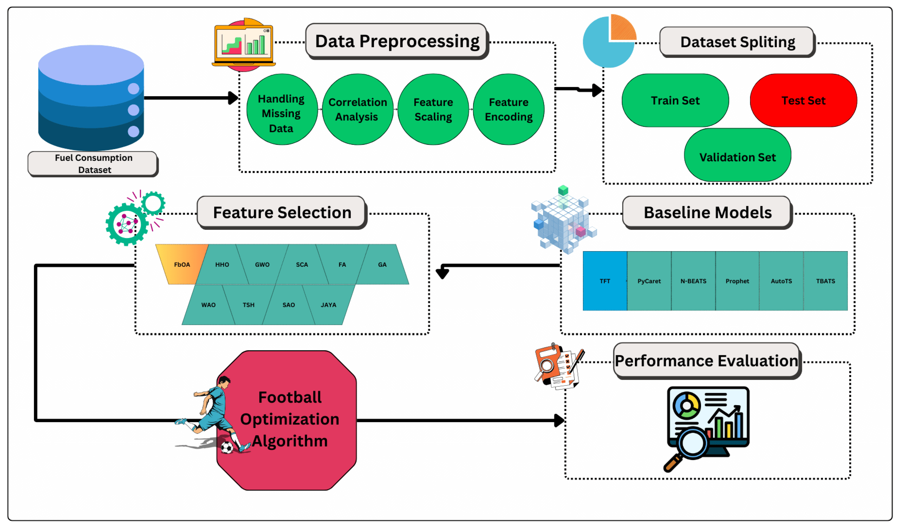
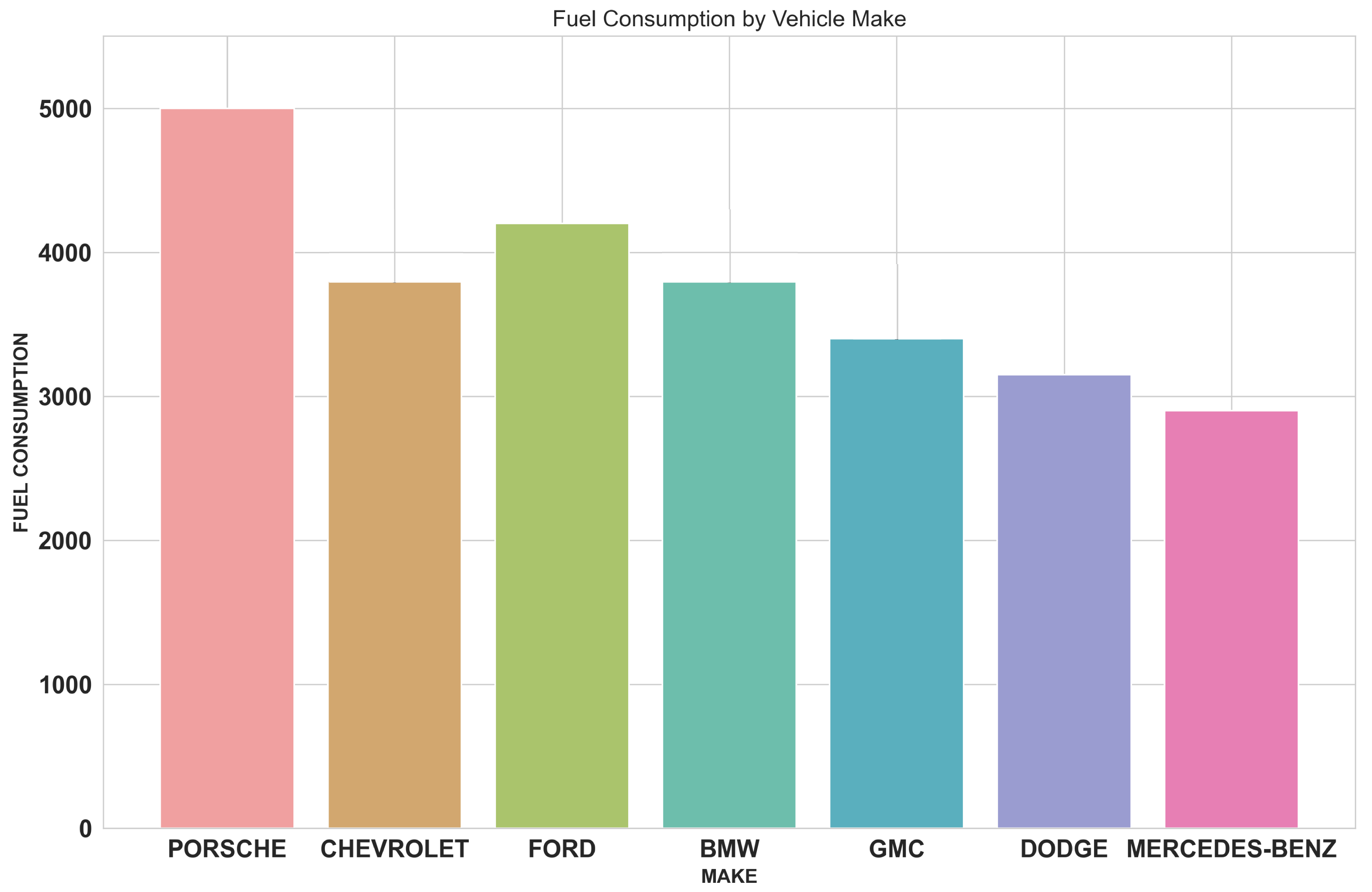
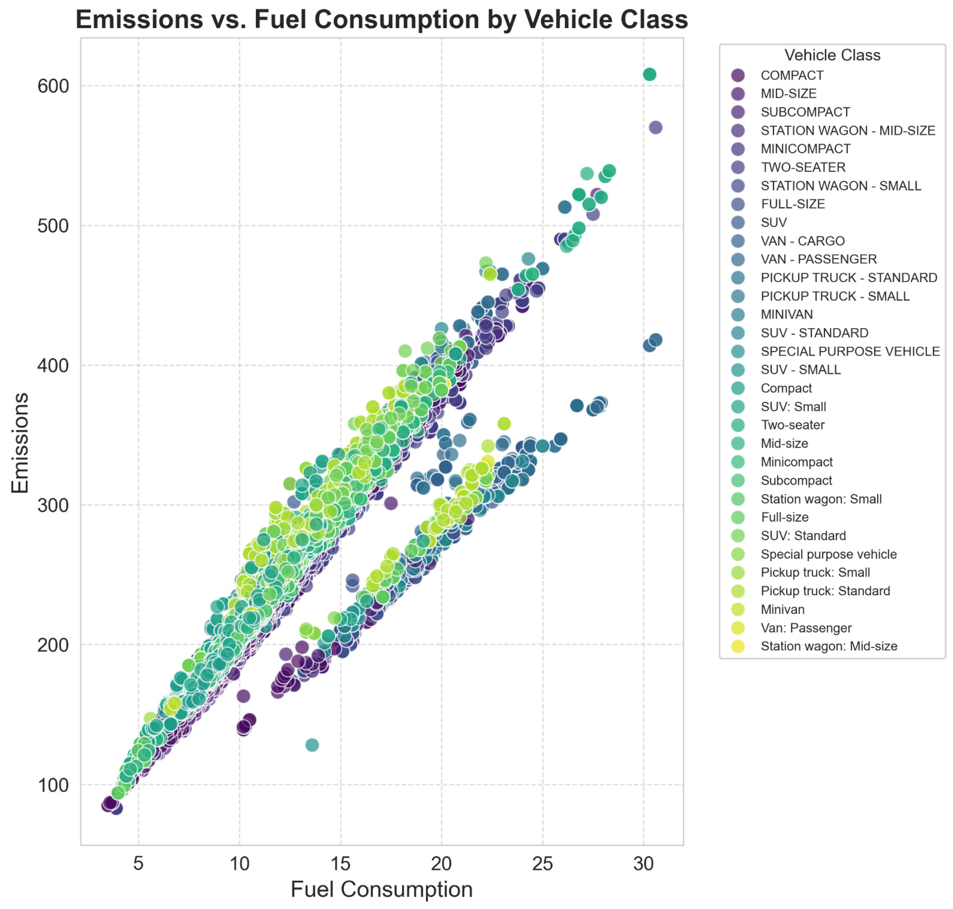
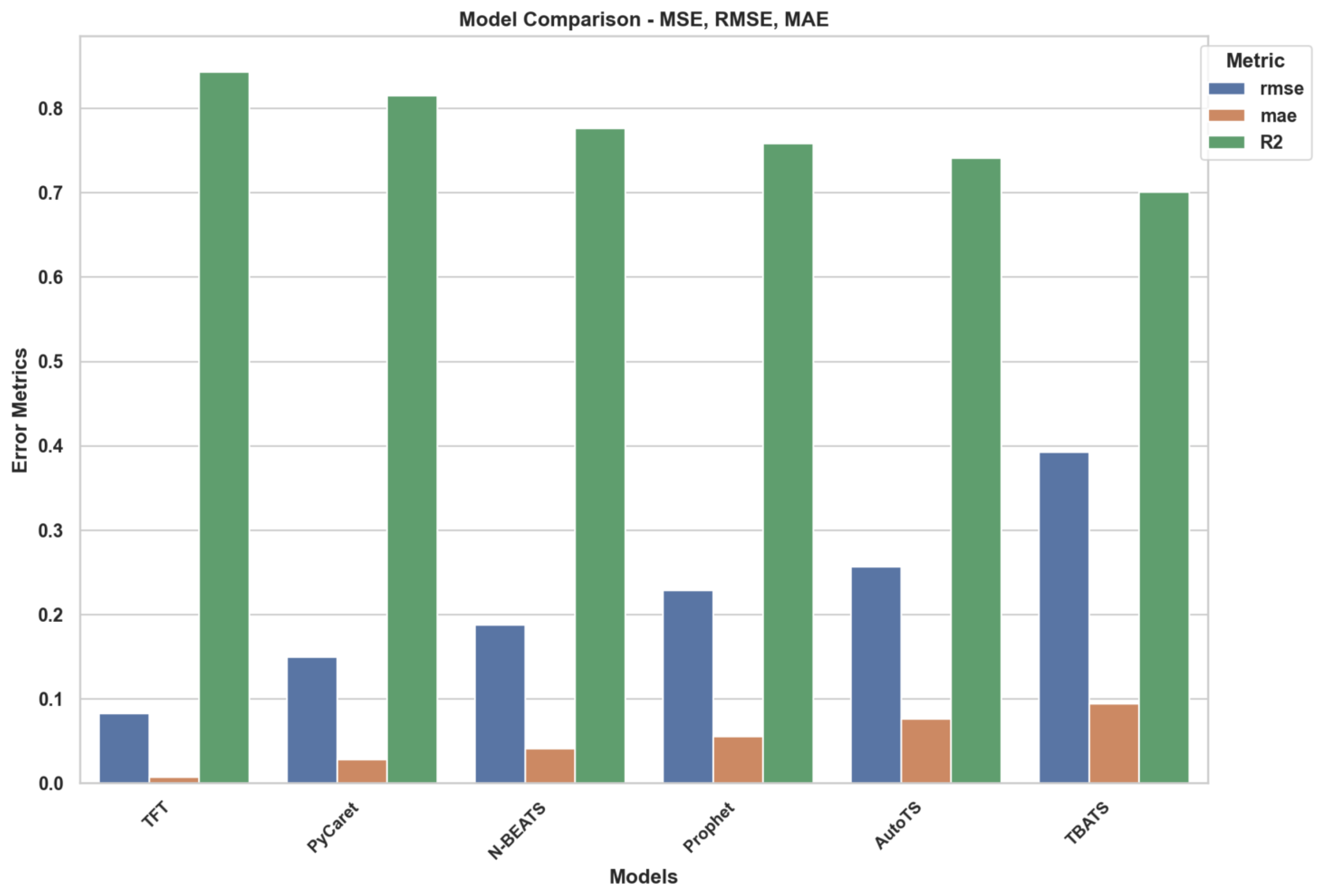
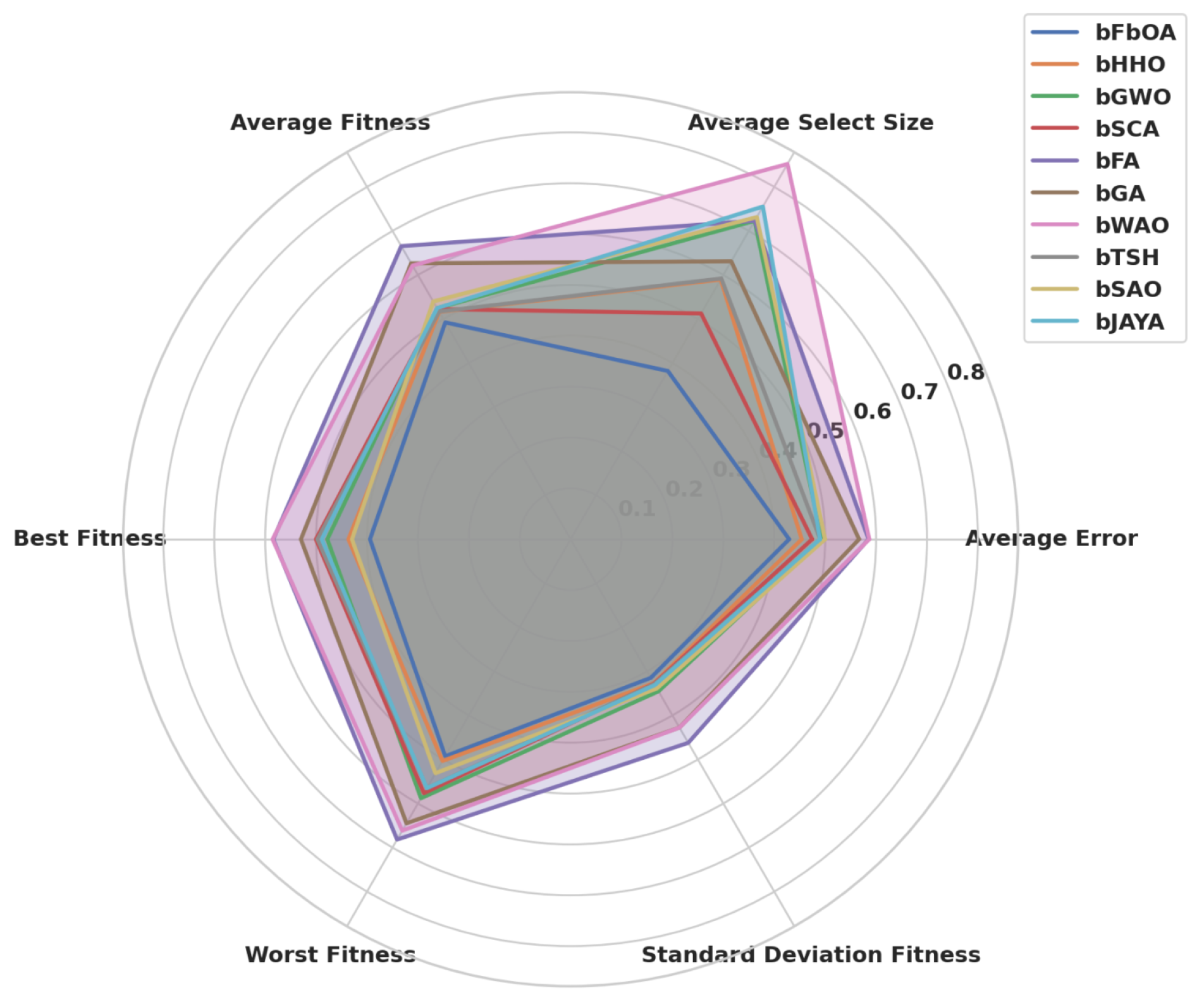
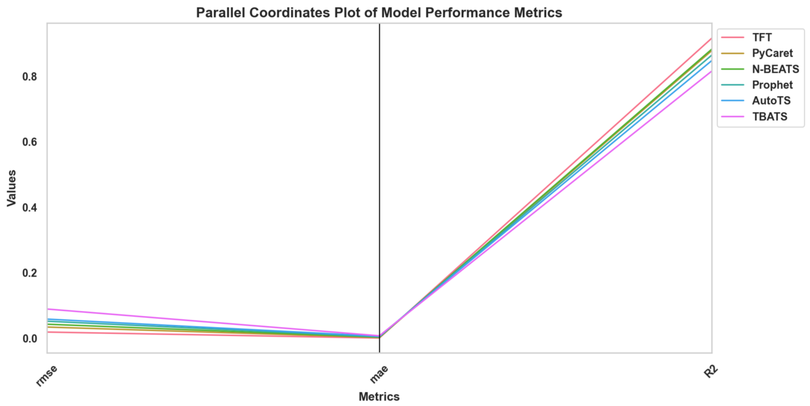
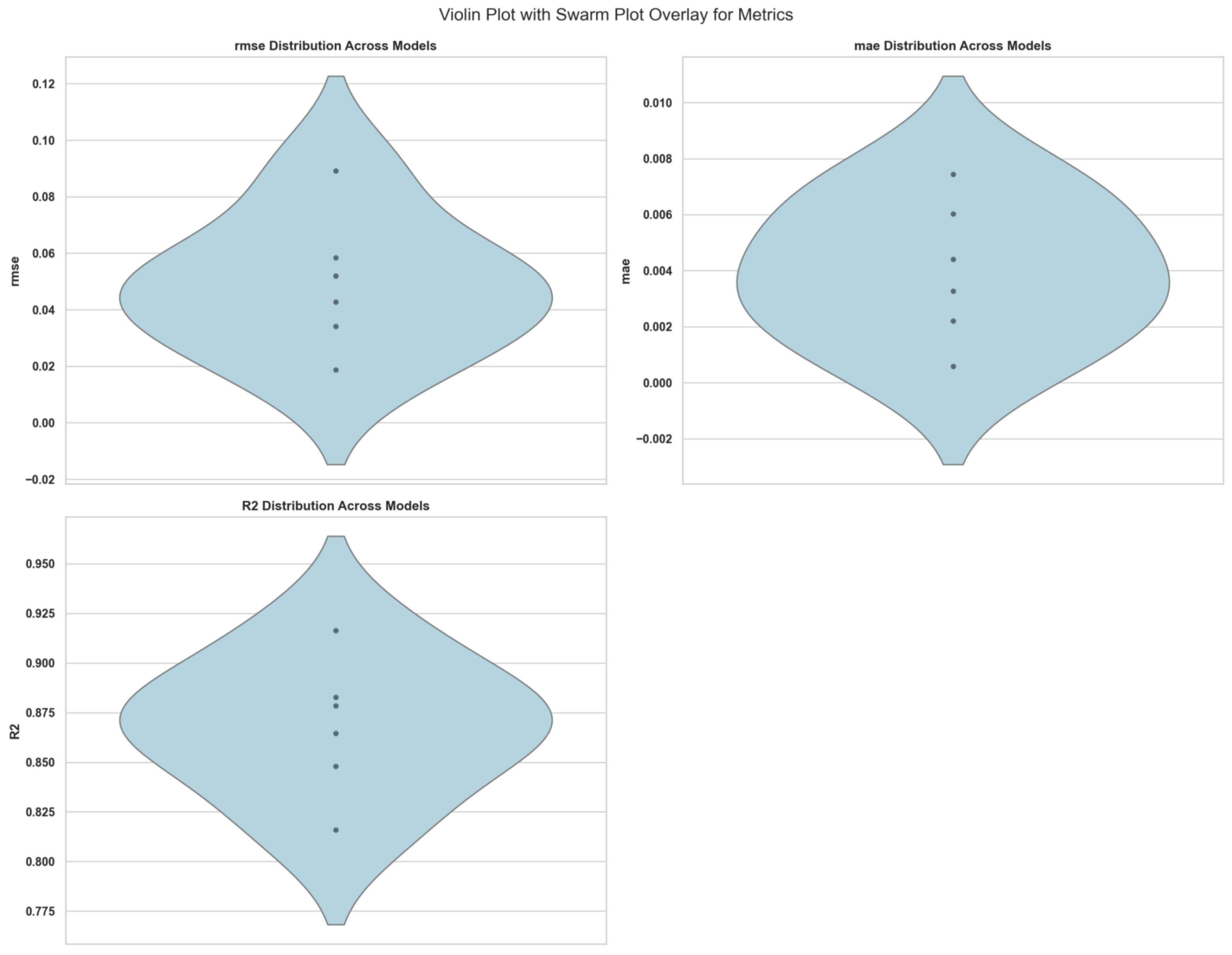
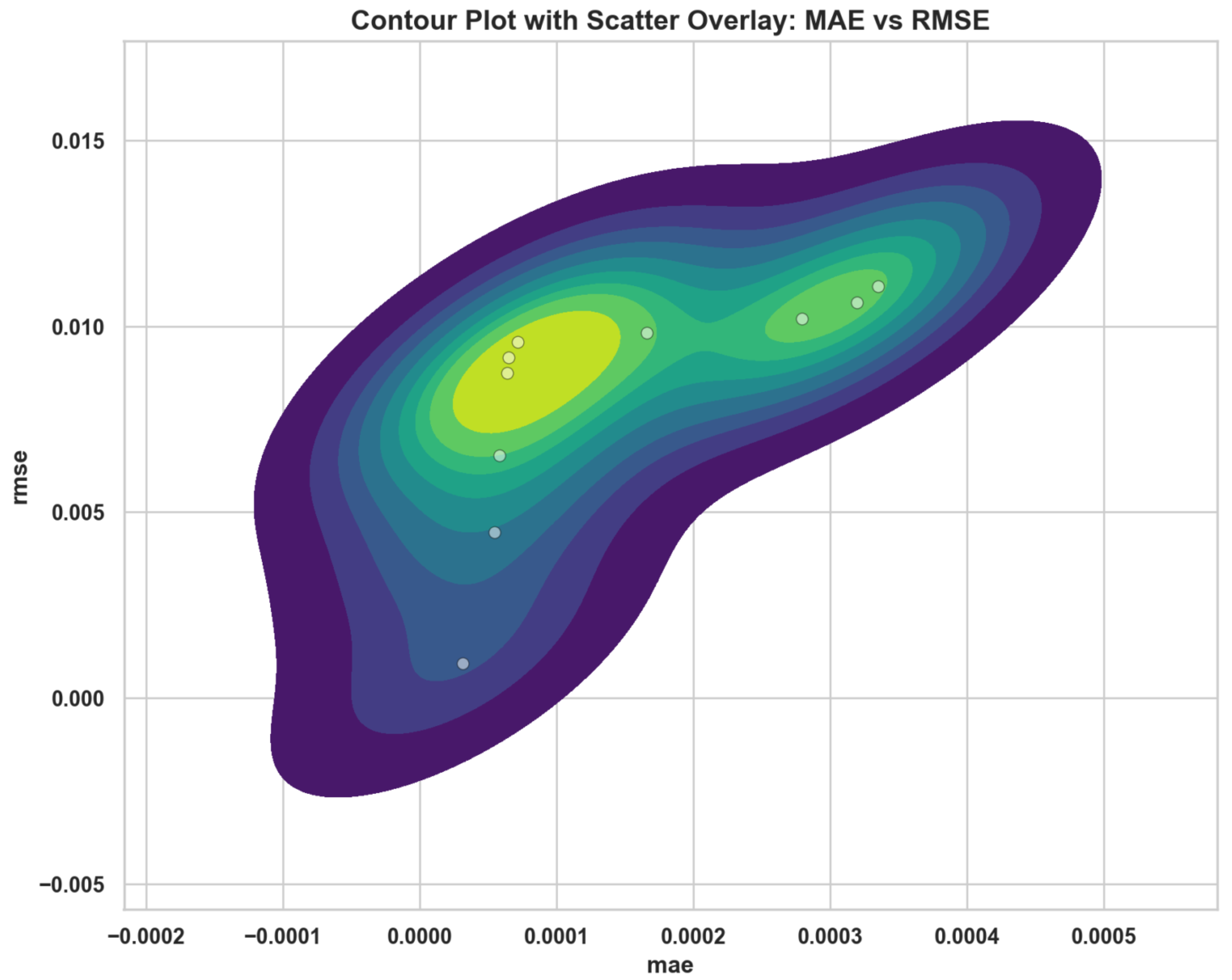
7. Conclusions

The contribution of this study was an advanced framework for predicting CO₂ emissions in light-duty vehicles through ML models trained using feature selection and hyperparameter optimization using a metaheuristic-based approach. The empirical results showed substantial reductions in root mean squared error (RMSE) for all optimized models, and hence the predicted accuracy was significantly improved. It is noticeable that the Football Optimization Algorithm (FbOA) yielded the best overall performance regarding the error rates and the correlation coefficient. Integrating metaheuristic optimization methods further increased model reliability by reducing overfitting, selecting better features, and increasing the generalization capabilities of ML models. These findings place a stronger emphasis on the impact of advanced optimization techniques on emissions forecasting and their application in environmental analytics.

The optimized models significantly increase predictive accuracy and computational efficiency and can be used for real-world implementation in transportation policy, automotive engineering, and environmental sustainability. The proposed framework offers more precise emissions forecasts, which policymakers can use to draft stricter laws regarding emission regulations, help automotive manufacturers design fuel-efficient cars, and help consumers make a judicious buying choice by taking account of the car’s emission rating. In addition, by including ML models with optimized features in intelligent transportation systems, they will be able to engage in real-time emissions monitoring which can further help in carrying out sustainable urban mobility programs and contribute to alleviating the issue of climate change at the global level.

There are many avenues to take in the future as a result of this study. One other possible direction explores developing the hybrid metaheuristic optimization techniques by utilizing many evolutionary algorithms to enhance the feature selection and hyperparameter resolution. Additionally, the real-time implementation of the optimized models in vehicular emissions monitoring systems can yield dynamic insights into the emissions trends in an adaptive regulatory measure in real-time. Next, after discussing the performance evaluation, scalability analysis is carried out to assess the performance of the proposed framework when deployed on large-scale datasets as it explores the framework’s scalability and applicability across a wide range of transportation systems. These future research aims will strengthen the adaptability and usefulness of the emissions prediction models to the extent that they will contribute to the timely development of sustainable transportation solutions.