Abstract
In this paper, we consider a modified Benjamin–Bona–Mahony (BBM) equation, which, for example, arises in shallow-water models. We discuss the well-posedness of the Dirichlet initial-boundary-value problem for the BBM equation. Our focus is on identifying a time-dependent source based on integral observation. First, we reformulate this inverse problem as an equivalent direct (forward) problem for a nonlinear loaded pseudoparabolic equation. Next, we develop and implement two efficient numerical methods for solving the resulting loaded equation problem. Finally, we analyze and discuss computational test examples.
Keywords:
Benjamin–Bona–Mahony equation; inverse source problem; integral observation; pseudoparabolic loaded equation; finite difference scheme MSC:
65M06; 65M22
1. Introduction
The Benjamin–Bona–Mahony (BBM) equation is a fundamental model in nonlinear wave theory, particularly for describing long waves in dispersive media. It was originally introduced as an improvement to the Korteweg–de Vries equation [1], offering better well-posedness properties while still capturing essential wave dynamics, such as surface waves in shallow water and internal waves in stratified fluids [2]. Beyond fluid dynamics, the BBM equation is also applied in plasma physics and nonlinear acoustics, where it models wave propagation in dispersive media with greater stability [3].
The BBM equation belongs to the class of nonlinear pseudoparabolic equations of the Sobolev type. This equation and its various modifications have been extensively studied by numerous authors. For example, the decay of solutions of the generalized BBM equation is investigated in [4], while the unique continuation for a linearized BBM equation is defined and analyzed in [5]. The authors of [6] apply Rothe’s fixed point theorem to establish the interior approximate controllability of a BBM-type equation with impulses and delay. The approximate controllability of the impulsive functional BBM equation with a nonlinear term involving a spatial derivative is proven in [7]. Properties related to control and energy dissipation for the BBM equation are discussed in [8].
Many numerical methods have been developed for solving both 1D and 2D BBM-type equations [9,10,11,12,13]. The finite volume-difference method is constructed in [9]. A fully discrete finite difference scheme with efficient convolution-based artificial boundary conditions for solving the Cauchy problem for the 1D linearized BBM equation is derived and theoretically analyzed in [13]. High-order accurate finite difference approximation, for a modified BBM equation is constructed in [11]. The approach is based on the use of high-order accurate summation-by-parts finite difference operators for the spatial discretization and explicit fourth-order accurate Runge–Kutta method in time. In [12], an explicit asymmetric three-layer second-order difference scheme is proposed for solving the BBM problem. A three-level conservative finite difference scheme is constructed and analyzed in [10] for solving a generalized BBM equation. A fully discrete finite difference scheme with efficient convolution-based artificial boundary conditions for solving the Cauchy problem associated with the 1D linearized BBM equation is derived and theoretically analyzed in [13]. High-order finite difference approximation for a modified BBM equation is constructed in [11]. In [12], an explicit asymmetric three-layer second-order difference scheme is proposed for solving the BBM problem. A three-level conservative finite difference scheme is constructed and analyzed in [10] for solving a generalized BBM equation.
One of the well-studied modifications of the BBM equation is the Benjamin–Bona–Mahony–Burgers (BBMB) equation, which incorporates viscous dissipation. Numerical methods are presented to solve the BBMB equation, for instance, in [14,15,16]. The authors of [14] develop a three-layer fourth-order implicit finite difference scheme that preserves energy dissipation for solving the 2D BBMB. In [15], a Crank–Nicolson-type finite difference scheme is constructed for the 1D BBMB equation. In [16], a second-order linearized finite difference scheme is developed to solve the 1D BBMB equation. The authors of [17] develop a spectral scheme, applying the transformed generalized Jacobi polynomial combined with the explicit fourth-order Runge–Kutta method for time integration.
Problems for differential equations in which both the solution and certain unknown parameters of the mathematical model must be determined are known as inverse problems; see, e.g., [18,19,20,21,22,23]. In this study, the unknown parameter is a time-dependent source in a modified BBM equation. Similar problems, though for linear or nonlinear parabolic, elliptic, or hyperbolic equations, have been extensively investigated; see, e.g., [18,19,20,21,22,23,24]. Notably, a considerable number of studies have focused on inverse problems for parabolic equations using an integral condition as additional information; see, e.g., [21,24,25,26,27]. The integral condition can represent total energy, average temperature, total mass of impurities, total flux, moments, and other physical quantities.
Currently, there are no known publications specifically addressing the solution of inverse source problems with integral observation for the BBM-type equation. Our goal in this paper is to partially fill this gap. However, there are studies on similar inverse problems for pseudoparabolic equations, which are closely related to the BBM equation. For instance, in [28], the authors discuss recovering the time-dependent source coefficient in a semilinear pseudoparabolic equation with a Neumann boundary condition from integral measurements. Using Rothe’s method, they prove the existence and uniqueness of a weak solution and construct a numerical time-discrete scheme, which is also analyzed. In [29], the inverse problem for determining an unknown time-dependent potential coefficient in a linear pseudoparabolic equation from nonlocal overdetermination conditions is considered. The authors establish uniqueness and the Lipschitz conditional stability of the inverse problem and develop an iterative algorithm for its solution. In [30], the authors investigate an inverse source pseudoparabolic problem with a p-Laplacian and integral observation. They prove the global and local in-time existence of solutions using the Galerkin method. Sufficient conditions for blow-up of the local solutions are derived, and the asymptotic behavior of the solutions to the inverse problem is explored.
In our previous papers [31,32], numerical methods are proposed for recovering a time-dependent boundary function in a two-dimensional linear pseudoparabolic equation using integral observations. In [32], the integral observation is imposed only on the part of the domain boundary. The well-posedness of both direct and inverse problems is also discussed.
Existence and uniqueness results for the direct and inverse time-dependent source problems for a time-fractional pseudo-parabolic equation with final time data are presented in [33]. The solvability of the inverse problem for the identification of a space-dependent source in a linear pseudoparabolic equation with final time measurements is studied in [34]. The authors of [35] investigate the well-posedness of an inverse space-dependent source problem for linear pseudoparabolic equations with a memory term and additional measurements at the final time. The problem is solved numerically by applying extended cubic B-spline functions and formulating it as a nonlinear least-squares minimization with Tikhonov regularization.
The paper [36] focuses on the identification of unknown parameters in a quasi-linear pseudoparabolic equation with periodic boundary conditions. The authors prove the existence and uniqueness of the solution and construct an implicit finite difference scheme.
The main contributions of this paper are as follows:
- -
- Proving the well-posedness of the Dirichlet initial-boundary-value problem for a modified BBM equation.
- -
- Formulating the inverse problem for identifying a time-dependent source based on integral measurements and establishing its well-posedness.
- -
- Reformulating the inverse source problem as a direct Dirichlet initial-boundary-value problem for a nonlinear loaded pseudoparabolic equation.
- -
- Developing and comparing two numerical methods for solving the inverse source problem.
Our motivation for the present study arises from both the practical applicability of the considered model and the mathematical challenge it poses—both theoretically and numerically.
The remainder of this paper is organized as follows. In the next section, we introduce the direct problem for the BBM equation and study its well-posedness. Section 3 formulates the source identification inverse problem and discusses its solution by reducing it to the direct problem. In Section 4, we develop two numerical methods for solving the inverse problem. The numerical results from test examples are presented in Section 5. Finally, the paper concludes with remarks and future research directions.
2. The BBM Model
In this section, we introduce the model problem and establish its well-posedness.
2.1. Problem Formulation
We consider the modified BBM equation [2,37].
with the initial condition
and the boundary conditions
The BBM equation appears in various physical models and plays a significant role in the theory and applications of long waves in nonlinear dispersive processes. It describes various physical phenomena, including long-wavelength surface oscillations in liquids, wave propagation in cold plasma environments (hydromagnetic waves), compressible fluid dynamics involving acoustic-gravity modes, and lattice vibrations (acoustic waves) in idealized harmonic crystal structures [38].
When the constant is known and the functions , , , , and are given, the problem (1)–(3) is well defined; see, e.g., [18,20,21,22].
This initial-boundary-value problem, referred to as the direct (or forward) problem, has been extensively studied in the literature. For instance, the existence of solutions for the modified BBM equation has been established in [3,39,40,41].
2.2. Well-Posedness
In this subsection, we discuss the existence and uniqueness of regular solutions to the problem (1)–(3). We apply the Galerkin method following the investigations in [39] and the results presented in [3] (Chapter 4).
Let denote the Sobolev space of order s, where s is a non-negative integer. In particular, corresponds to the standard space, equipped with the inner product and the norm .
Furthermore, we define as the Banach space of integrable functions , such that belongs to , with the norm
and
For later use, we require the following inequality: [3,18]
where , denotes the usual norm in , and the constant C is independent of v.
Additionally, we require the Agmon inequality
We now apply the Galerkin method to establish the existence and uniqueness of a solution to (1)–(3).
Proof.
We adopt the proof of Theorem 1.1 from [39], where the Cauchy problem with compact support is studied.
First, we consider the case of homogeneous Dirichlet boundary conditions, i.e., . We seek an approximate solution to Equation (1) in the form outlined in Step (i) of [39]:
where we assume that are linearly independent and that their finite linear combinations are dense in .
The functions are determined from the system of ordinary differential equations (ODEs)
where
The ODE system (7), solved with the initial conditions converges to strongly in as m goes to infinity, and are constants.
Since the coefficient matrix of is invertible, we can prove the local existence and uniqueness of the ODE system (7) in the same manner as in [39]. Step (ii) provides a priori estimates, which guarantee the global solution on .
To derive a priori estimates for the problem (1)–(3), it is convenient to rewrite them with zero boundary conditions:
where
We solve this equation with the initial condition
and the boundary conditions
The unknown functions are the same as in (6) and can be determined from the system ODEs
Now, as an a priory estimate in [39] (Step (ii)), we derive the estimate
3. The Inverse Problem
In this section, we discuss the solution to the time-dependent source identification inverse problem. We consider Equation (1), assuming that the function is unknown, and the integral observation is given by
3.1. Reformulation of the Inverse Problem to a Direct One
We reduce the the inverse problem (1)–(3), (9) into a direct problem, assuming the existence of all necessary continuous derivatives. We differentiate Equation (9) with respect to t and use (1) to express in the resulting equation. This leads to the following expression:
Now, we replace on the right-hand side of (1) with formula (10) to obtain the new equation for the unknown function .
So, we transform the inverse problem (1)–(3) and (9) to the loaded nonlinear pseudoparabolic Equation (11), subject the initial conditions (2) and boundary conditions (3).
In contrast to various studies on linear loaded parabolic and pseudoparabolic equations (see, e.g., [20,21,23,25,42,43,44,45,46,47]), the differential operator incorporates internal or boundary values of the solution or its first derivatives, while Equation (11) includes a mixed second-order derivative. Specifically, in [25,42,43,45,46,47] the linear loaded operator involves the solution values at the interior points of the domain, while in [44], both the solution and the temporal derivative of the solution are involved in the differential operator.
The work [28] examines a semilinear pseudoparabolic problem (including the BBM equation), where the differential operator involves an integral of the solution.
The loaded Equation (11) differs from those studied in the existing literature.
3.2. The Well-Posedness of the Reduced Problem
In this subsection, we study the existence, uniqueness, and regularity of the solution to (11), subject to the initial conditions (2) and the boundary conditions (3), using the Galerkin method. The following assertion holds.
Theorem 2.
Proof.
The proof follows the line of reasoning in [39]. We seek a solution to (11), that satisfies the following system of ODEs:
Now, we choose the system , in such a way that the coefficient matrix of is invertible. We then proceed as in Theorem 1, following the approach outlined in [39]. □
4. Numerical Solution to the Direct Problem
In this section, we develop second-order-in-space-and-time finite difference schemes for solving (1)–(3) assuming that the differential problem solution is sufficiently smooth for performing the corresponding operations.
We consider the uniform spatial and temporal meshes
and denote and .
Let }. We use the inner product and norm
Further, we introduce the difference approximation [48] of continuously differential functions up to the second order
the discrete seminorm and norm , , and -norm
Let be the bilinear form
We approximate the nonlinear term in (1) on the basis of the representation
where .
Thus, using (12), the initial-boundary-value problem (1)–(3) is discretized with the Crank–Nicolson finite difference scheme
Here, , where .
We use some results from [15] to prove the following assertion.
Theorem 3.
Proof.
For simplicity, without loss of generality, we take zero boundary conditions for (13). Next, fixing n, we express Equation (13) in the following form:
which requires the continuous mapping :
We perform the inner product of Equation (14) with U and use Lemma 1 in [15] to find
Applying the Cauchy inequality to the last term, we obtain
where C is a generic constant depending on and .
Furthermore, using a discrete Sobolev embedding inequality, we find
Therefore, for
we have , and from Lemma 2 in [15] follows the existence of an approximate solution to the scheme (13).
Now, applying the Cauchy inequality and then the Sobolev embedding discrete inequality to the last term, we obtain
Then, as in [15], the discrete Gronwall inequality and the discrete Sobolev inequality give the global boundness of the discrete solution
where is a constant that may depend only on the input data.
In order to solve the nonlinear system of difference Equation (13), avoiding the iteration process, we use the quasi-linearization
5. Numerical Solution to the Inverse Problem
In this section, we develop two algorithms for solving the inverse problem (1)–(3), (9). Both methods are based on second-order linearized discretization (16). The first algorithm employs an iterative procedure for g, which is common for solving non-local problems. The second approach is an iteration-free approach.
First, we approximate in (10) at . Applying second-order discretizations for the derivatives, we obtain
where
and the quantity is obtained exactly or numerically, depending on the function :
Numerical method 1 (NM1). At each time layer, we solve (16) for , obtained from (17) at the corresponding iteration k. Specifically, we determine iteratively, starting with an initial guess . Assume that . At each time layer, for , we compute
Then, we update the value of g at time layer
For , we set . The iteration process continues until the desired accuracy is achieved, i.e.,
Note that if an iterative procedure is used to solve the nonlinear system of difference Equation (13), such as Newton’s or Picard’s method, then solving the corresponding system (18) will involve two nested iterations—an outer and an inner loop.
Proposition 1.
Proof.
The coefficient matrix of (18) is the same as that of the direct problem (16). Under restriction (19), it is a tridiagonal, diagonally dominant matrix. Indeed, let and . Then, we have
Taking into account (15) and the boundary conditions, we conclude that the coefficient matrix of (18) is a diagonally dominant matrix and, therefore, invertible. This ensures the solvability of the inverse problem using MN1. □
- Numerical method 2 (NM2). This approach is based on the discretization of (11). We approximate this differential equation in the same way as (16), avoiding an iterative procedure, and apply discretization (17) to approximate . The resulting finite difference scheme iswhereThe coefficient matrix of (21) is sparse, but not tridiagonal; see Figure 1. Moreover, the diagonal domination cannot be guaranteed only for a large-space step size . For example, for , we have
 Figure 1. Coefficient matrix structure of (21), I = 20.
In order to overcome this computational disadvantage, we apply the decomposition technique [43]. We rewrite the system (21) in the form
where
Next, we represent the solution in the form
6. Computational Results
In this section, we assess the accuracy and efficiency of both numerical methods, NM1 and NM2, for solving the inverse problem (1)–(3), (9). We provide the results for exact and noisy measurements (9). For comparison, we also present the computational results for the direct problem (1)–(3), solved by the finite difference scheme (16).
The errors and order of convergence are presented in maximum and discrete norms:
All computations are performed for a fixed ratio , i.e., , and for the stopping criteria of the iteration process in NM1, we set .
Example 1 (Direct problem).

In this example, we present the computational results for the direct problem (1)–(3), as they will serve as a benchmark for evaluating the numerical accuracy of the inverse problem solution. Table 1 displays the errors and corresponding orders of convergence. The numerical experiments confirm that the accuracy of the finite difference scheme (16) is .
Table 1.
Errors and convergence rates of solution u, direct problem, Example 1.
Example 2 (Inverse problem problem: exact data).
In the numerical experiments, the measured function in (9) is derived directly from the exact solution. The results presented in Table 1 and Table 2 show both the accuracy and convergence rates for the reconstructed data and the computed solution u, obtained using MN1 and NM2, respectively.
Table 2.
Errors and convergence rates of the recovered function g and solution u, NM1, Example 2.
Additionally, we provide the CPU time and the average number of iterations () required by NM1 to achieve the desired accuracy . The results indicate that the recovered source and the solution u exhibit second-order accuracy in both time and space, in both the maximum and norms. The precision of the restored and solution u is comparable for both methods; however, NM1 requires significantly more CPU time than NM2 due to the iterative process.
Figure 2 illustrates the accuracy of the recovered source and the solution u in the maximum and norms (left), as well as the average number of iterations and the corresponding CPU time (right) for different values of , NM1, and . Although the number of iterations is relatively high, it decreases as the mesh is refined or when the required accuracy is reduced. For this example, if is approximately greater than , the accuracy improves insignificantly, and similarly, the increase in the number of iterations and CPU time becomes negligible.
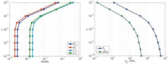
Figure 2.
Errors of the solution u and the recovered source versus the precision (left), and CPU time and average number of iterations versus the precision (right), NM1, , Example 2.
The numerical experiments demonstrate that NM2 is significantly more efficient than NM1. Comparing the results in Table 1 with those in Table 1 and Table 3, we can conclude that, as expected, the numerical solution obtained by solving the direct problem with the exact is more accurate than the one computed by solving the inverse problem for the reconstructed source . Nevertheless, the accuracy achieved through the inverse problem remains sufficiently high, and the convergence rate is preserved.
Table 3.
Errors and convergence rates of the recovered function g and solution u, NM2, Example 2.
Example 3.
(Inverse problem: noisy data) In these tests, we deal with noisy measurements
where ρ is the noise level and represents random values, uniformly distributed on the interval . To generate the values of , we approximate using central finite difference approximation in time for , and left and right second-order approximations similar to those in (17). We apply polynomial curve fitting of degree 5 to smooth the data.
In Table 4 and Table 5, we present the accuracy of the recovered source and solution u for different levels of noise, obtained using NM1, with , and NM2, with for both methods. As in Example 1, the accuracy achieved by both methods is similar, but NM1 operates more slowly due to the iterative process. We observe that the restoration achieves satisfactory precision even with perturbed data. The numerically recovered time-dependent source is sufficiently accurate to ensure that the solution u achieves optimal accuracy.
Table 4.
Errors of the numerically recovered source g and solution u, NM1, Example 3.
Table 5.
Errors of the numerically recovered source g and solution u, NM2, Example 3.
In Figure 3 and Figure 4, we present the exact function g and its recovered counterpart obtained using NM2, along with the corresponding errors for and , respectively. Figure 5 illustrates the exact and recovered functions g for , computed using NM1 and NM2. In Figure 6, the solution u recovered by NM2 and the corresponding error across the entire computational domain are depicted.
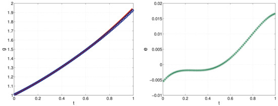
Figure 3.
Exact source (solid red line) and numerically recovered (line with blue circles), (left), and the corresponding error (right), NM2, Example 3.
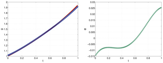
Figure 4.
Exact source (solid red line) and numerically recovered (line with blue circles), (left), and the corresponding error (right), NM2, Example 3.
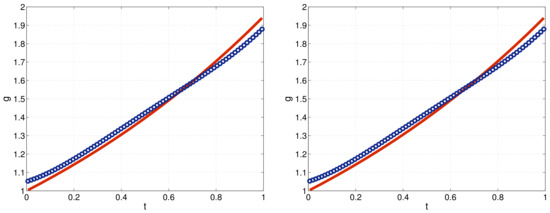
Figure 5.
Exact source (solid red line) and numerically recovered (line with blue circles); , NM1 (left), and , NM2 (right), Example 3.
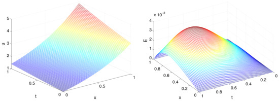
Figure 6.
Numerical solution u and the corresponding error in the space–time domain, , NM2, Example 3.
7. Conclusions
In this work, we considered the initial-boundary-value problem for the Benjamin–Bona–Mahony equation and established the existence and uniqueness of its solution. We formulated and investigated an inverse problem for identifying the time-dependent source in the BBM equation. The inverse problem was reformulated as a direct problem for a loaded equation, and its well-posedness was discussed and justified. Based on this reformulation, we developed and compared two numerical methods for solving the problem. The computational results demonstrated that the proposed methods achieve second-order accuracy in both space and time for exact measurements. For noisy data, the recovery remains sufficiently precise. The numerically reconstructed time-dependent source is accurate enough to ensure the solution attains optimal accuracy.
Following the nature of the considered mathematical model for the BBM equation, our future work will continue with studying inverse coefficient and source problems for the Benjamin–Bona–Mahony–Burgers equation.
Author Contributions
Conceptualization, L.G.V. and M.N.K.; methodology, M.N.K. and L.G.V.; investigation, M.N.K. and L.G.V.; resources, M.N.K. and L.G.V.; writing—original draft preparation, M.N.K. and L.G.V.; writing—review and editing, L.G.V.; validation, M.N.K. All authors have read and agreed to the published version of the manuscript.
Funding
This study is financed by the European Union-NextGenerationEU, through the National Recovery and Resilience Plan of the Republic of Bulgaria, project № BG-RRP-2.013-0001.
Data Availability Statement
The data are contained within the article.
Conflicts of Interest
The authors declare no conflicts of interest.
References
- Bona, J.L.; Smith, R. The initial value problem for the Korteweg-de Vries equation. Philos. Trans. R. Soc. Lond. Ser. A Math. Phys. Sci. 1975, 278, 555–604. [Google Scholar] [CrossRef]
- Benjamin, T.B.; Bona, J.L.; Mahony, J.J. Model equations for long waves in nonlinear dispersive systems. Philos. Trans. Roy. Soc. Lond. Ser. A 1972, 272, 47. [Google Scholar]
- Larkin, N.A.; Novikov, V.A.; Ianenko, N.N. Nonlinear Equations of ‘Variable Type’; Izdatel’stvo Nauka: Novosibirsk, Russia, 1983; 272p. (In Russian) [Google Scholar]
- Albert, J. On the decay of solutions of the generalized Benjamin-Bona-Mahony equation. J. Math. Anal. Allps. 1989, 141, 527–537. [Google Scholar] [CrossRef]
- Zhang, X.; Zuazua, E. Unique continuation for the linearized Benjamin-Bona-Mahony equation with space-dependent potential. Math. Ann. 2003, 325, 543–582. [Google Scholar] [CrossRef][Green Version]
- Leiva, H.; Sanchez, J.L. Rothe’s fixed point theorem and the controllability of the Benjamin-Bona-Mahony equation with impulses and delay. Appl. Math. 2016, 7, 1748–1764. [Google Scholar] [CrossRef]
- Leiva, H. Controllability of the impulsive functional BBM equation with nonlinear term involving spatial derivative. Syst. Control. Lett. 2017, 109, 12–16. [Google Scholar] [CrossRef]
- Rosier, L.; Zhang, B.-Y. Unique continuation property and control for the Benjamin-Bona-Mahony equation on a periodic domain. J. Differ. Equ. 2013, 254, 141–178. [Google Scholar] [CrossRef]
- Amiraliev, G.M. Difference schemes for problems in the theory of dispersive waves. Dokl. Math. 1991, 42, 235–238. [Google Scholar]
- Berikelashvili, G.; Miranashvili, M. On the convergence of difference schemes for generalized Benjamin-Bona-Mahony equation. Numer. Methods Partial. Differ. Equ. 2013, 30, 301–320. [Google Scholar] [CrossRef]
- Kjelldahl, V.; Mattsson, K. Numerical simulation of the generalized modified Benjamin-Bona-Mahony equation using SBP-SAT in time. J. Comput. Appl. Math. 2025, 459, 116377. [Google Scholar] [CrossRef]
- Saul’ev, V.K.; Chernikov, A.A. A solution by the finite difference method of a nonlinear regularized equation of shallow water. Differ. Uravn. 1983, 19, 1818–1820. [Google Scholar]
- Zheng, Z.; Pang, G.; Ehrhardt, M.; Liu, B. A fast second-order absorbing boundary condition for the linearized Benjamin-Bona-Mahony equation. Numer. Algorithms 2025, 98, 2037–2080. [Google Scholar] [CrossRef]
- Cheng, H.; Wang, X. A high-order linearized difference scheme preserving dissipation property for the 2D Benjamin-Bona-Mahony-Burgers equation. J. Math. Anal. Appl. 2021, 500, 125182. [Google Scholar] [CrossRef]
- Omrani, K.; Ayadi, M. Finite difference discretization of the Benjamin-Bona-Mahony-Burgers equation. Numer. Methods Partial. Differ. Equ. 2008, 24, 239–248. [Google Scholar] [CrossRef]
- Zhang, Q.; Liu, L.; Zhang, J. The numerical analysis of two linearized difference schemes for Benjamin-Bona-Mahony-Burgers equation. Numer. Methods Partial. Differ. Equ. 2020, 26, 1790–1810. [Google Scholar] [CrossRef]
- Zhou, Y.; Jiao, J. Spectral method for one dimensional Benjamin-Bona-Mahony-Burgers equation using the transformed generalized Jacobi polynomial. Math. Model. Anal. 2024, 29, 509–524. [Google Scholar] [CrossRef]
- Hasanov, A.H.; Romanov, V.G. Introduction to Inverse Problems for Differential Equations, 1st ed.; Springer: Cham, Switzerland, 2017; 261p. [Google Scholar]
- Isakov, V. Inverse Problems for Partial Differential Equations, 3rd ed.; Springer: Cham, Switzerland, 2017; p. 406. [Google Scholar]
- Kabanikhin, S.I. Inverse and Ill-Posed Problems; DeGruyer: Berlin, Germany, 2011. [Google Scholar]
- Lesnic, D. Inverse Problems with Applications in Science and Engineering; CRC Press: Abingdon, UK, 2021; p. 349. [Google Scholar]
- Prilepko, A.I.; Orlovsky, D.G.; Vasin, I.A. Methods for Solving Inverse Problems in Mathematical Physics; Marcel Dekker: New York, NY, USA, 2000. [Google Scholar]
- Samarskii, A.A.; Vabishchevich, P.N. Numerical Methods for Solving Inverse Problems of Mathematical Physics; Walter de Gruyter: Berlin, Germany, 2007; 452p. [Google Scholar]
- Prilepko, A.I.; Kamynin, V.L.; Kostin, A.B. Inverse source problem for parabolic equation with the condition of integral observation in time. J. Inverse Ill-Posed Probl. 2018, 26, 523–539. [Google Scholar] [CrossRef]
- Cannon, J.R.; Lin, Y.; Wang, S. Determination of a control parameter in a parabolic partial differential equation. J. Aust. Math. Soc. Ser. B Appl. Math. 1991, 33, 149–163. [Google Scholar] [CrossRef]
- Cannon, J.R. The solution of the heat equation subject to the specification of energy. Quart. Appl. Math. 1963, 21, 155–160. [Google Scholar] [CrossRef]
- Vasin, I.A.; Kamynin, V.L. Asymptotic behaviour of the solutions of inverse problems for parabolic equations with irregular coefficients. Sb. Math. 1997, 188, 371–387. [Google Scholar] [CrossRef]
- Van Bockstal, K.; Khompysh, K. A time-dependent inverse source problem for a semilinear pseudo-parabolic equation with Neumann boundary condition. arXiv 2025, arXiv:2502.04821. [Google Scholar]
- Fu, J.-L.; Liu, J. Recovery of a potential coefficient in a pseudoparabolic system from nonlocal observation. Appl. Numer. Math. 2023, 184, 121–136. [Google Scholar] [CrossRef]
- Khompysh, K.; Huntul, M.J.; Shazyndayeva, M.K.; Iqbal, M.K. An inverse problem for pseudoparabolic equation: Existence, uniqueness, stability, and numerical analysis. Quaest. Math. 2024, 47, 1979–2001. [Google Scholar] [CrossRef]
- Koleva, M.N.; Vulkov, L.G. Numerical determination of a time-dependent boundary condition for a pseudoparabolic equation from integral observation. Computation 2024, 12, 243. [Google Scholar] [CrossRef]
- Koleva, M.N.; Vulkov, L.G. The numerical solution of an inverse pseudoparabolic problem with a boundary integral observation. Mathematics 2025, 13, 908. [Google Scholar] [CrossRef]
- Ruzhansky, M.; Serikbaev, D.; Torebek, B.T.; Tokmagambetov, N. Direct and inverse problems for time-fractional pseudo-parabolic equations. Quaest. Math. 2021, 45, 1071–1089. [Google Scholar] [CrossRef]
- Nikolaev, O.Y. Solvability of the linear inverse problem for the pseudoparabolic equation. Math. Notes NEFU 2023, 30, 58–66. [Google Scholar]
- Huntul, M.J.; Khompysh, K.; Shazyndayeva, M.K.; Iqbal, M.K. An inverse source problem for a pseudoparabolic equation with memory. AIMS Math. 2024, 9, 14186–14212. [Google Scholar] [CrossRef]
- Baglan, I.; Kanca, F.; Mishra, V.N. Fourier method for an existence of quasilinear inverse pseudo-parabolic equation. Iran. J. Math. Sci. Inform. 2024, 19, 193–209. [Google Scholar] [CrossRef]
- Bona, J.L.; Tzvetkov, N. Sharp well-posedness for the BBM equation. Discret. Contin. Dyn. Syst. 2009, 23, 1241–1252. [Google Scholar] [CrossRef]
- Belobo, D.B.; Das, T. Solitary and Jacobi elliptic wave solutions of the generalized Benjamin-Bona-Mahony equation. Commun. Nonlinear Sci. Numer. Simul. 2017, 48, 270–277. [Google Scholar] [CrossRef]
- Medeiros, L.A.; Miranda, M.M. Weak solutions for a nonlinear dispersive equation. J. Math. Anal. Appl. 1977, 59, 432–441. [Google Scholar] [CrossRef]
- Medeiros, L.A.; Miranda, M.M.; Medeiros, L.A.; Perla Menzala, G. On global solutions of a nonlinear dispersive equation of Sobolev type. Bol. Soc. Bras. Mat 1978, 9, 49–59. [Google Scholar] [CrossRef]
- Medeiros, L.A.; Perla Menzala, G. Existence and uniqueness for periodic solutions of the Benjamin-Bona-Mahony equation. SIAM J. Math. Anal. 1977, 8, 792–799. [Google Scholar] [CrossRef]
- Abdullayev, V.M.; Aida-zade, K.R. Finite-difference methods for solving loaded parabolic equations. Comput. Math. Math. Phys 2016, 56, 93–105. [Google Scholar] [CrossRef]
- Bondarev, E.A.; Voevodin, A.F. A finite difference method for solving initial-boundary value problems for loaded differential and integro-differential equations. Differ. Equ. 2000, 36, 1711–1714. [Google Scholar] [CrossRef]
- Kandilarov, J.D.; Valkov, R.L. A numerical approach for the American call option pricing model. In Numerical Methods and Applications; Dimov, I., Dimova, S., Kolkovska, N., Eds.; NMA 2010. Lecture Notes in Computer Science; Springer: Berlin/Heidelberg, Germany, 2011; Volume 6046, pp. 453–460. [Google Scholar]
- Koleva, M.N.; Vulkov, L.G. Reconstruction of time-dependent right-hand side in parabolic equations on disjoint domains. J. Phys. Conf. Ser. 2023, 2675, 012025. [Google Scholar] [CrossRef]
- Koleva, M.N.; Vulkov, L.G. Reconstruction of the time-dependent diffusion coefficient in a space-fractional parabolic equation. In New Trends in the Applications of Differential Equations in Sciences; Slavova, A., Ed.; NTADES 2023. Springer Proceedings in Mathematics & Statistics; Springer: Cham, Switzerland, 2024; Volume 449. [Google Scholar]
- Nakhusher, A.M. Loaded Equations and Applications; Nauka: Moscow, Russia, 2012. (In Russian) [Google Scholar]
- Samarskii, A.A. The Theory of Difference Schemes; Nauka: Moscow, Russia; Marcel Dekker, Inc.: New York, NY, USA; Basel, Switzerland, 2001. (In Russian) [Google Scholar]


Disclaimer/Publisher’s Note: The statements, opinions and data contained in all publications are solely those of the individual author(s) and contributor(s) and not of MDPI and/or the editor(s). MDPI and/or the editor(s) disclaim responsibility for any injury to people or property resulting from any ideas, methods, instructions or products referred to in the content. |
© 2025 by the authors. Licensee MDPI, Basel, Switzerland. This article is an open access article distributed under the terms and conditions of the Creative Commons Attribution (CC BY) license (https://creativecommons.org/licenses/by/4.0/).