Elastic Wave Propagation Through Cylinders with Fluid-Filled Fractures Using the Discontinuous Galerkin Method

Abstract

Accurately modeling fractures in wave-propagation simulations is challenging due to their small scale relative to other features. While equivalent-media models can approximate fracture-induced anisotropy, they fail to capture their discrete influence on wave propagation. To address this limitation, the Interior-Penalty Discontinuous Galerkin Method (IP-DGM) can be adapted to incorporate the Linear-Slip Model (LSM) to represent fractures explicitly. In this study, we apply IP-DGM to elastic wave propagation in fractured cylindrical domains using realistic fracture compliances obtained from laboratory experiments (using ultrasonic-pulse transmission) to simulate the effects of fluid-filled fractures. We analyze how fracture spacing and fluid type influence P- and S-wave behavior, focusing on amplitude attenuation and wave-front delays. Our numerical results align with experimental and theoretical predictions, demonstrating that higher-density fluids enhance wave transmission, reducing the impedance contrast and improving coupling across fracture surfaces. These findings highlight the capability of IP-DGM to accurately model wave propagation in realistic fractured and saturated media, providing a valuable tool for seismic monitoring in fractured reservoirs and other applications where fluid-filled fractures are prevalent.

1. Introduction

Elastic wave propagation through fractured media is critical in oil and gas exploration, geothermal energy, CO₂ sequestration, non-destructive evaluation of materials, and many other applications. Accurately characterizing the subsurface requires understanding how fractures and their infill influence elastic waves. However, incorporating fractures into numerical simulations is challenging because their scale is often smaller than the grid size used in numerical modeling [1]. Consequently, various approaches have been developed to represent fractures in elastic wave simulations, each with drawbacks.

A common approach to simulating wave propagation in fractured media is to use an equivalent medium, replacing the fractured domain with an effective homogeneous medium with overall equivalent properties [2,3]. While this method simplifies computations, it fails to capture the discrete effects of fractures on elastic waves. In this approach, the fractures are smoothed out and, therefore, it is unsuitable when fracture spacing is comparable to or larger than the wavelength, as single and sparsely spaced fractures can significantly affect wave propagation [4].

An alternative approach is to explicitly model fractures within wave-equation simulations, preserving their mechanical influence on elastic waves. For this purpose, various numerical methods have been developed for modeling wave propagation: the Finite-Difference Method (FDM) is widely used, but it struggles with discontinuities at interfaces [5,6]. Traditional finite element methods are also popular [7], but struggle to capture the discrete nature of fractures, especially when dealing with fluid-filled fractures where wave behavior depends on mechanical and hydraulic properties. The Spectral Element Method (SEM) provides high accuracy, but it assumes that the wave field is continuous at element interfaces [8,9]. The Discontinuous Galerkin Method (DGM), although computationally expensive, is well suited for discrete fractures due to its ability to handle any type of discontinuities in the wave field [10,11,12].

The Linear Slip Model (LSM) proposed by Schoenberg [2] has been widely used to model fractures as interfaces with discontinuous displacements. LSM was first implemented into DGM by De Basabe et al. [11] using the Interior-Penalty Discontinuous Galerkin Method (IP-DGM) for elastic wave propagation. IP-DGM explicitly models fractures without averaging their effects, preserving their discrete influence by incorporating LSM to accurately capture localized fracture dynamics, enabling more flexible and precise elastic wave simulations across complex geometries and fluid conditions. A related implementation using the Nodal Discontinuous Galerkin method was developed by Möller and Friederich [13], where fractures with various rheologies are modeled via additional numerical fluxes based on LSM.

DGM is a robust numerical approach to simulate wave propagation in fractured media. Its ability to explicitly represent fractures makes it well-suited for modeling complex fracture geometries while minimizing numerical dispersion. A recent study by Pyrak-Nolte [14] used DGM to model wave propagation across single fractures in a 2D isotropic medium, systematically examining how fracture geometry influences wave attenuation. Other studies, such as Pyrak-Nolte et al. [15] and Rioyos-Romero [16], have compared the effects of discrete fractures on seismic anisotropy using LSM and the effective moduli method. Their findings confirmed that the effective moduli method loses the discrete nature of fractures, whereas LSM captures the anisotropy and preserves the localized effects of fractures on wave propagation. In an elastic medium with parallel fractures, wave velocities and transmission coefficients depend on wave frequency, fracture stiffness-to-seismic impedance ratio, and angle of incidence effects that are lost in effective-medium models unless modified with complex moduli, which changes the medium from elastic to viscoelastic.

The flexibility of DGM in handling discontinuities has also enabled its integration with other high-accuracy methods to expand its applicability. For instance, Vamaraju et al. [17] developed a Hybrid Galerkin Method (HGM) that combines DGM with the Spectral Element Method, applying DGM only in regions containing fracture while using SEM elsewhere. This approach maintains the strength of DGM in modeling fracture-induced discontinuities while improving overall computational efficiency, demonstrating the adaptability of the method to complex, heterogeneous models where fractures are spatially localized. In addition, Duru et al. [12] extended DGM to complex 3D media by developing an energy-stable, high-order formulation using physics-based fluxes and curvilinear adaptive meshes, enhancing both stability and accuracy.

Compliance is a key parameter in LSM used to characterize fractures by defining the relationship between stress and displacement discontinuities across the fracture interface. Numerical simulations usually use compliance values that are either unrealistic or exceed those reported in the literature [11]. Other studies relying on assumed or theoretical compliance values, such as [11,18,19], may not fully capture the complexities of real fractured media.

A key aspect of this work lies in explicitly incorporating laboratory-derived fracture compliance data into IP-DGM for elastic wave simulations. Unlike previous studies that rely on assumed or unrealistic fracture properties, our approach ensures that the numerical model closely reflects physical experiments, capturing the effects of fluid-filled fractures more accurately.

In this paper, we apply IP-DGM to investigate the effects of fluid-filled fractures on elastic wave propagation, explicitly modeling fractures using LSM. We incorporate laboratory data (fracture compliances) that characterize fluid-filled fractures within IP-DGM, and analyze how fracture spacing and different fluid types influence P- and S-wave propagation, capturing key physical behaviors such as attenuation and wave delays. The paper is structured as follows: Section 2 presents the mathematical formulation, including the governing equations, and a review of LSM in wave modeling. Section 3 describes the numerical implementation and simulation results. Section 4 discusses the implications of our findings, and Section 5 concludes with key points and potential applications.

2. Mathematical Model Formulation

This section summarizes the governing equations and the methodology implemented by De Basabe et al. [10,11]. This summary provides the necessary background for understanding the computational framework used in our numerical experiments.

2.1. Governing Equations: The Elastic Wave Equation

An elastic wave is generated when particles in a medium are set in motion by a mechanical perturbation. It represents the response of the medium as it seeks to restore the particles to their original positions. This section presents the fundamental equations governing elastic wave propagation, starting with the momentum equation for an elastic continuum:

$$\rho \ddot{\mathcal{U}}=\mathbf{\nabla }·\mathit{\sigma }+\mathit{f},$$

(1)

where $\mathcal{U}=\mathcal{U}(\mathit{x},t)$ is the displacement field, $\ddot{\mathcal{U}}={\partial }^2\mathcal{U}/\partial t^2$ is the acceleration, $\rho =\rho \left(\mathit{x}\right)$ denotes the density, $\mathit{\sigma }=\mathit{\sigma }(\mathit{x},t)$ is the stress tensor, and $\mathit{f}(\mathit{x},t)$ represents the source vector. We require a relationship between stress and strain, which is given by Hooke’s law:

$$\mathit{\sigma }=\mathit{C}:\mathit{ϵ},$$

(2)

where $\mathit{C}$ is the fourth-order stiffness tensor or the elasticity tensor, the operator: denotes the double-dot product, and $\mathit{ϵ}$ is the strain tensor, defined in terms of the displacement by

$$\mathit{ϵ}={\displaystyle \frac{1}{2}}\left(\nabla \mathcal{U}+\nabla {\mathcal{U}}^T\right).$$

(3)

For linear, isotropic media, the stress–strain relationship, Equation (2), takes the following form:

$${\sigma }_{ij}\left(\mathcal{U}\right)=\lambda {\delta }_{ij}{\partial }_k{\mathcal{U}}_k+\mu ({\partial }_i{\mathcal{U}}_j+{\partial }_j{\mathcal{U}}_i),$$

(4)

where $\lambda =\lambda \left(\mathit{x}\right)$ and $\mu =\mu \left(\mathit{x}\right)$ are the Lamé parameters and ${\delta }_{ij}$ is Kronecker’s delta. Substituting Equation (4) into Equation (1) yields the elastic wave equation for an isotropic and elastic domain in vector notation:

$$\begin{array}{cccc}\hfill \rho \ddot{\mathcal{U}}-\nabla \lambda (\nabla ·\mathcal{U})-\nabla \mu (\nabla \mathcal{U}+\nabla {\mathcal{U}}^T)& =\mathit{f}\hfill & \hfill & \mathrm{in}\Omega \times (0,T]\hfill \\ \hfill \mathit{\tau }\left(\mathcal{U}\right)& =0\hfill & \hfill & \mathrm{on}\partial \Omega \hfill \\ \hfill \mathcal{U}=\dot{\mathcal{U}}& =0\hfill & \hfill & \mathrm{for}t=0,\hfill \end{array}$$

(5)

where $\Omega \subset {\mathbb{R}}^d$ is the physical domain, d is the number of physical dimensions (2 or 3), $\mathit{\tau }\left(\mathcal{U}\right)=\mathbf{\sigma }\left(\mathcal{U}\right)·\mathit{n}$ is the traction vector, $\partial \Omega$ is the external boundary of $\Omega$, $\mathit{n}$ is a unitary vector normal to $\partial \Omega$, and $(0,T]$ is the time domain.

2.2. The Linear Slip Model

Schoenberg [2] originally proposed the Linear Slip Model (LSM) to represent a fracture embedded in an elastic background. In this model, a fracture is considered planar and infinitely long, with a small thickness compared to the elastic wavelength [2]. This kind of fracture is treated mathematically as a boundary condition in the elastic wave equation, where the stresses are continuous across the fracture, but the displacements are not [2]. The magnitude of the discontinuity or jump in the displacement field $\left[\mathcal{U}\right]$ is linearly related to the traction vector ${\mathit{\tau }}^{\gamma }$ at the surface of $\gamma$ through the fracture compliance $\mathit{Z}$ as follows:

$$\left[\mathcal{U}\right]=\mathit{Z}{\mathit{\tau }}^{\gamma },$$

(6)

where $[.]$ denotes the function jump, $\gamma$ corresponds to the fracture discontinuity, and the components $Z_{ij}$ of the fracture compliance matrix are given by [20]:

$$Z_{ij}=Z_N{n}_i{n}_j+Z_T({\delta }_{ij}-n_i{n}_j),$$

(7)

where $Z_N$ is the normal fracture compliance, $Z_T$ is the tangential fracture compliance, and $n_i$ are the components of a vector normal to the fracture.

LSM is derived in a purely elastic context and is suitable for fractures filled with solids or fluids. This model has been validated through laboratory experiments [4,21,22,23]. The compliance matrix $\mathit{Z}$ is the inverse of the fracture stiffness, often used to parameterize the fracture. In this work, the normal and tangential compliances are determined from laboratory experiments using the ultrasonic pulse technique [4,21,23,24,25]. These values were obtained for fractures filled with different fluids: air, water, silicon oil, and honey. Estimations involve analyzing the elastic wave measurements (seismograms) obtained from the ultrasonic transmission tests, where compliance values are obtained by correlating the transmission coefficients of compressional and shear waves incident normally on the fractures [4,26]. We assume that the effect of fluids on wave propagation is inherently incorporated into the estimated compliance values, allowing us to use them directly in our modeling approach.

2.3. Elastodynamic Modeling in Fractured Media

Fractures are incorporated into the elastic wave equation (Equation (5)) by introducing the LSM condition (Equation (6)) within the weak formulation, employing IP-DGM. This type of finite element method approximates solutions using discontinuous, piecewise polynomial basis functions. IP-DGM allows for discontinuities across the elements, ensuring proper coupling through interface conditions. This enables accurate modeling of wave propagation across fractured media.

Let us introduce the necessary notation, following [10,11]. Let ${\Omega }_h$ be a finite element partition of the domain $\Omega$, ${\Gamma }_h$ the set of all faces between the elements in ${\Omega }_h$, ${\Gamma }_c\subset {\Gamma }_h$ the subset of all faces where the displacement field is continuous and ${\Gamma }_f\subset {\Gamma }_h$ the subset of faces representing fractures, where ${\Gamma }_c\cup {\Gamma }_f={\Gamma }_h$ and ${\Gamma }_c\cap {\Gamma }_f=\varnothing$, and $\gamma$ is an edge between elements. Also, $\{.\}$ denotes the average of the function at $\gamma \in {\Gamma }_h$, given by

$$\left\{u\right\}={\displaystyle \frac{1}{2}}\left({u|}_{E_1}{+u|}_{E_2}\right),$$

(8)

for a scalar function u on $\gamma$, which is the edge between the elements $E_1$ and $E_2$. To obtain the weak formulation of Equation (5), we introduce the vector space $\mathbf{X}=X^d$, where $X=span{\left\{{\varphi }_i\right\}}_{i=1}^N$, ${\varphi }_i$ are the discontinuous basis functions and N is the total number of these functions.

The first step to find $\mathit{u}$∈$\mathbf{X}$ is to multiply Equation (5) by a vector test function $\mathit{v}\in \mathbf{X}$, and integrate element-wise to obtain

$${\partial }_{tt}{\int }_E\rho \mathit{u}·\mathit{v}d\mathit{x}-{\int }_E(\nabla \lambda (\nabla ·\mathit{u})·\mathit{v}-\nabla \mu (\nabla \mathit{u}+\nabla {\mathit{u}}^T)·\mathit{v})d\mathit{x}={\int }_E\mathit{f}·\mathit{v}d\mathit{x}.$$

(9)

Recalling the Gauss divergence theorem corollary:

$${\int }_{\Omega }\phi \nabla ·\mathit{u}={\int }_{\partial \Omega }\phi \mathit{u}·\mathit{n}-{\int }_{\Omega }\nabla \phi ·\mathit{u},$$

(10)

where $\mathit{n}$ is a unitary vector normal to $\partial \Omega$, we apply it to Equation (9) and obtain the corresponding equation with boundary terms

$$\begin{array}{cc}\hfill {\partial }_{tt}{\int }_E\rho \mathit{u}·\mathit{v}d\mathit{x}& +{\int }_E\left(\lambda (\nabla ·\mathit{u})(\nabla ·\mathit{v})+\mu (\nabla \mathit{u}+\nabla {\mathit{u}}^T):\nabla \mathit{v}\right)d\mathit{x}\hfill \\ \hfill & -{\int }_{\gamma }\left(\lambda (\nabla ·\mathit{u})\mathit{v}+\mu \mathit{v}(\nabla \mathit{u}+\nabla {\mathit{u}}^T)\right)·\mathit{n}d\gamma \hfill \\ \hfill & ={\int }_E\mathit{f}·\mathit{v}d\mathit{x}.\hfill \end{array}$$

(11)

Since $\mathit{u}$ is discontinuous across element boundaries $\gamma$, the boundary integral is not well defined, but we can define jump and average operators across element interfaces when we add over all the elements in ${\Omega }_h$. Using the property $\left[\xi \psi \right]=\left\{\xi \right\}\left[\psi \right]+\left[\xi \right]\left\{\psi \right\}$ for $\gamma \in {\Gamma }_c$, yields

$$\begin{array}{ccc}\hfill & & {\mathit{J}}_{\gamma }^c(\mathit{u},\mathit{v})={\left.-{\int }_{\gamma }(\lambda (\nabla ·\mathit{u})\mathit{v}+\mu \mathit{v}(\nabla \mathit{u}+\nabla {\mathit{u}}^T))·\mathit{n}d\gamma \right|}_{E_1}\hfill \\ & & {\left.-{\int }_{\gamma }(\lambda (\nabla ·\mathit{u})\mathit{v}+\mu \mathit{v}(\nabla \mathit{u}+\nabla {\mathit{u}}^T))·\mathit{n}d\gamma \right|}_{E_2}=-{\int }_{\gamma }\left\{{\mathit{\tau }}^{\gamma }\left(\mathit{u}\right)\right\}·\left[\mathit{v}\right]+\left\{\mathit{v}\right\}·\left[{\mathit{\tau }}^{\gamma }\left(\mathit{u}\right)\right]d\gamma \hfill \\ & & -{\int }_{\gamma }(\left\{{\mathit{\tau }}^{\gamma }\left(\mathit{v}\right)\right\}·\left[\mathit{u}\right]+\left\{\mathit{u}\right\}·\left[{\mathit{\tau }}^{\gamma }\left(\mathit{v}\right)\right])d\gamma +{\displaystyle \frac{R}{\left|\gamma \right|}}{\int }_{\gamma }\{\lambda +2\mu \}\left[\mathit{u}\right]·\left[\mathit{v}\right]d\gamma .\hfill \end{array}$$

(12)

The symmetry and penalty terms were added without loss of generality and for stability, where R is the penalty and $\left|\gamma \right|$ is the size of $\gamma$. Due to the physical requirement of traction continuity across element interfaces, the jumps in the traction vector must be zero, $\left[{\mathit{\tau }}^{\gamma }\right]=0$; therefore,

$$\begin{array}{ccc}\hfill {\mathit{J}}_{\gamma }^c(\mathit{u},\mathit{v})& =& {\int }_{\gamma }\left\{{\mathit{\tau }}^{\gamma }\left(\mathit{u}\right)\right\}·\left[\mathit{v}\right]d\gamma -{\int }_{\gamma }\left\{{\mathit{\tau }}^{\gamma }\left(\mathit{v}\right)\right\}·\left[\mathit{u}\right]d\gamma +{\displaystyle \frac{R}{\left|\gamma \right|}}{\int }_{\gamma }\{\lambda +2\mu \}\left[\mathit{u}\right]·\left[\mathit{v}\right]d\gamma .\hfill \end{array}$$

(13)

Whenever $\gamma \in {\Gamma }_f$ the symmetry and penalty terms are not required since the displacement is discontinuous; therefore,

$${\mathit{J}}_{\gamma }^f(\mathit{u},\mathit{v})={\int }_{\gamma }\left\{{\mathit{\tau }}^{\gamma }\left(\mathit{u}\right)\right\}·\left[\mathit{v}\right]d\gamma .$$

(14)

Substituting the traction average in this equation with Equation (6) yields

$${\mathit{J}}_{\gamma }^f(\mathit{u},\mathit{v})={\int }_{\gamma }{\mathit{Z}}^{-1}\left[\mathit{u}\right]·\left[\mathit{v}\right]d\gamma .$$

(15)

Notice that the LSM condition is imposed weakly through this term, which is similar to a penalty term, but instead of a penalty, it uses the inverse of compliance. Also, if the compliances tend to zero, the penalty approaches infinity, effectively sealing the fracture. If the compliance is very large, this term vanishes, similar to a free-surface condition. It is assumed that fractures align with the element interface in the finite-element mesh to accurately simulate the discontinuity.

Summing over all elements in Equation (11) and substituting Equations (13) and (15), we obtain the IP-DGM weak formulation, given by the following statement:

• Find $u\in \mathbf{X}$ such that

$$\sum _{E\in {\Omega }_h}\left({\left(\rho {\partial }_{tt}\mathit{u},\mathit{v}\right)}_E+{\mathit{B}}_E\left(\mathit{u},\mathit{v}\right)\right)+\sum _{\gamma \in {\Gamma }_c}{\mathit{J}}_{\gamma }^c(\mathit{u},\mathit{v})+\sum _{\gamma \in {\Gamma }_f}{\mathit{J}}_{\gamma }^f(\mathit{u},\mathit{v})=\sum _{E\in {\Omega }_h}{(\mathit{f},\mathit{v})}_E,\forall \mathit{v}\in \mathbf{X}$$

(16)

where

$$\begin{array}{ccc}\hfill {(\mathit{u},\mathit{v})}_E& =& {\int }_E\mathit{u}·\mathit{v}d\mathit{x},\hfill \end{array}$$

(17)

$$\begin{array}{ccc}\hfill {\mathit{B}}_E(\mathit{u},\mathit{v})& =& {\int }_E\left(\lambda (\nabla ·\mathit{u})(\nabla ·\mathit{v})+\mu (\nabla \mathit{u}+\nabla {\mathit{u}}^T):\nabla \mathit{v}\right)d\mathit{x}.\hfill \end{array}$$

(18)

This method was validated and tested by De Basabe et al. [11]. A detailed study on its accuracy and stability can be found in [10,27], where the authors compare different numerical schemes. It has also been successfully used for elastic wave propagation in fractured digital rocks in [16] and references therein.

3. Numerical Simulations

3.1. Model Parameters

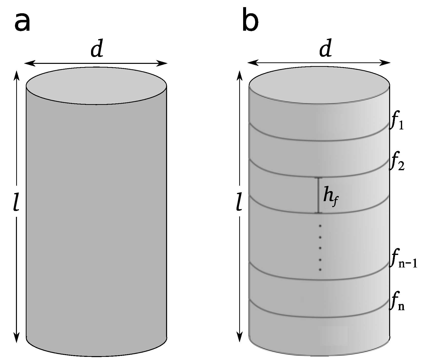
We numerically simulate the transmission of waves through parallel fractures orthogonal to the axes of a cylindrical domain, ensuring that the models are digital twins of the laboratory experiments in Ramos-Barreto et al. [28]. The 3D model we consider, shown in Figure 1, represents a cylinder with a height of 76.08 mm and a diameter of 38 mm. Its elastic properties are as follows: density $\rho =2702$ kg/m³, P-wave velocity $V_p=6432$ m/s and S-wave velocity $V_s=3133$ m/s. We consider four different models: one intact (without fractures, used as a reference) and three with varying spacings between fractures. We consider four fluid types filling the fractures: air, water, silicon oil, and honey. The respective densities are listed in

Table 1. Fluid densities.

Fluid	Density (kg/m3)
Air (dry)	1.20 [29]
Silicon Oil	965.00 [30]
Water	998.20 [31]
Honey	1420.00 [32]

. The fracture parameters for the different models, obtained from laboratory experiments using the ultrasonic pulse technique, are provided in

Table 2. Fracture parameters for the numerical experiments with fluid-filled fractures; $h_f$ is the spacing between fractures.

${\mathit{h}}_{\mathit{f}}$ (mm)	Fluid	${\mathit{Z}}_{\mathit{N}}$ (m/Pa)	${\mathit{Z}}_{\mathit{T}}$ (m/Pa)
38.08	Air	$5.874\times {10}^{-14}$	$1.767\times {10}^{-14}$
	Water	$9.300\times {10}^{-15}$	$1.691\times {10}^{-14}$
	Sil. Oil	$1.124\times {10}^{-14}$	$3.761\times {10}^{-14}$
	Honey	$9.319\times {10}^{-15}$	$1.628\times {10}^{-14}$
12.68	Air	$4.743\times {10}^{-14}$	$1.486\times {10}^{-14}$
	Water	$5.991\times {10}^{-15}$	$1.487\times {10}^{-14}$
	Sil. Oil	$9.207\times {10}^{-15}$	$1.933\times {10}^{-14}$
	Honey	$4.749\times {10}^{-15}$	$1.495\times {10}^{-14}$
6.84	Air	$3.953\times {10}^{-14}$	$1.534\times {10}^{-14}$
	Water	$7.148\times {10}^{-15}$	$1.555\times {10}^{-14}$
	Sil. Oil	$1.117\times {10}^{-14}$	$1.977\times {10}^{-14}$
	Honey	$4.963\times {10}^{-15}$	$1.276\times {10}^{-14}$

.

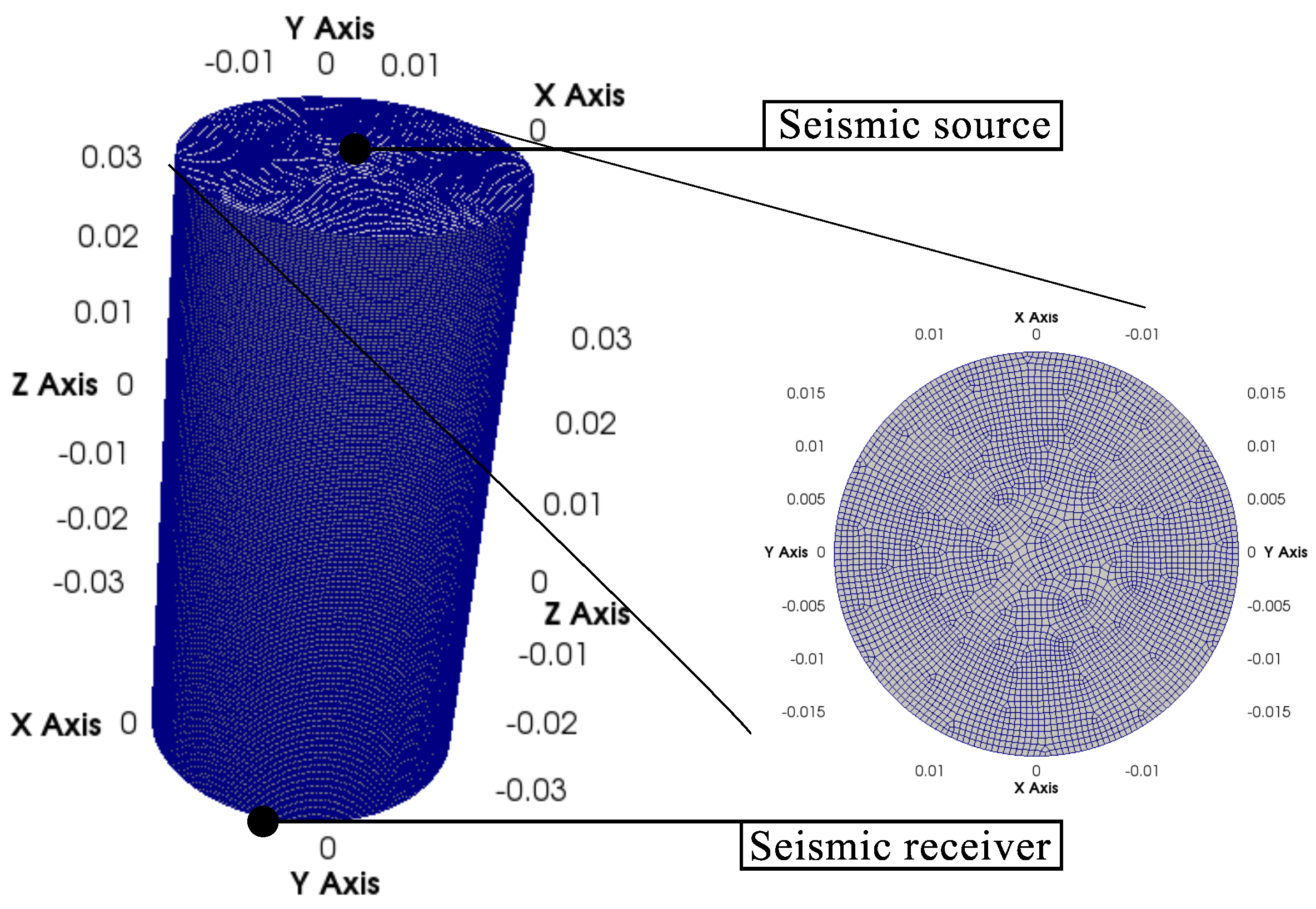
The 3D simulations were conducted in a Cartesian coordinate system ($x,y,z$). The 3D cylindrical mesh used in the numerical simulations was generated using the software Cubit (Cubit Version 13.1, Sandia National Laboratories, https://cubit.sandia.gov (accessed on 11 April 2025)) (Figure 2). The mesh consists of 807,030 hexahedral elements, carefully designed to ensure that the fractures coincide with interfaces between elements, explicitly incorporating them into the simulations. The element’s edges range between 0.36 mm and 0.54 mm. The element sizes were chosen to minimize numerical dispersion, ensuring sampling ratios of at least 5 nodes per wavelength for the S-waves and at least 11 nodes per wavelength for P-waves.

The wave source is modeled as a vector point source centered at the top of the model. The shape of the time function is a Ricker wavelet (the second derivative of a Gaussian distribution) with a peak frequency of 1 MHz. The time-stepping scheme used for the numerical experiments is second-order finite differences, with a time step of $\Delta t=4\times {10}^{-10}$ s. The P- and S-wavelengths are 6.43 mm and 3.13 mm, respectively.

3.2. Simulation Results

This section presents the results of numerical simulations of wave transmission through elongated fractures with three different fracture spacings and four types of infilled material. These simulations illustrate the effects of fluid type on the displacement field. In all experiments, the source is positioned at the top center of the cylinder, and we applied free-surface boundary conditions on its lateral surface.

The source is oriented according to the primary wave type we want to analyze. For the P-wave, the impulse acts in the z-direction, whereas for the S-wave, it acts in the x-direction. Both waves propagate parallel to the vertical axis, with particle motion occurring in the z-direction for the P-wave and the x-direction for the S-wave. Figure 3a,b show the magnitude of the displacement field for the source polarized in the x- and z-directions. For comparison, all the figures in this section are plotted using the same amplitude scale.

The following shows snapshots of the displacement field for different cases. We compare behavior under two conditions: (i) the same fluid with varying fracture spacing and (ii) the same fracture spacing with various fluids. Each case is examined separately for P- and S-waves. The snapshots represent the wavefields in the x-z plane, and the color scale indicates displacement amplitudes (blue for negative displacement and red for positive displacement).

To ensure meaningful comparison between wave types, the snapshots are taken at different times: t = 28 µs for P-waves and t = 49 µs for the S-waves. These times were selected based on the velocity ratio between P- and S-waves so that the wavefields are captured at comparable propagation distances.

3.3. Same Fluid with Varying Fracture Spacing

3.3.1. P-Wave Displacement Field

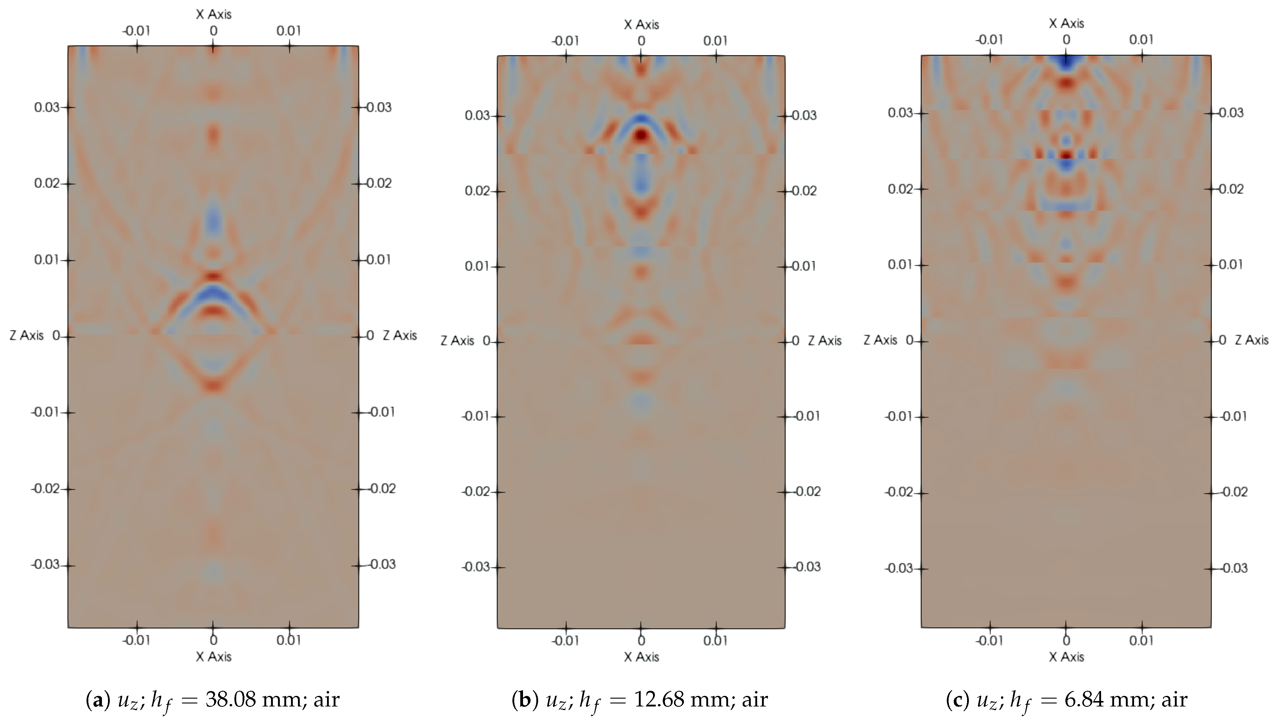
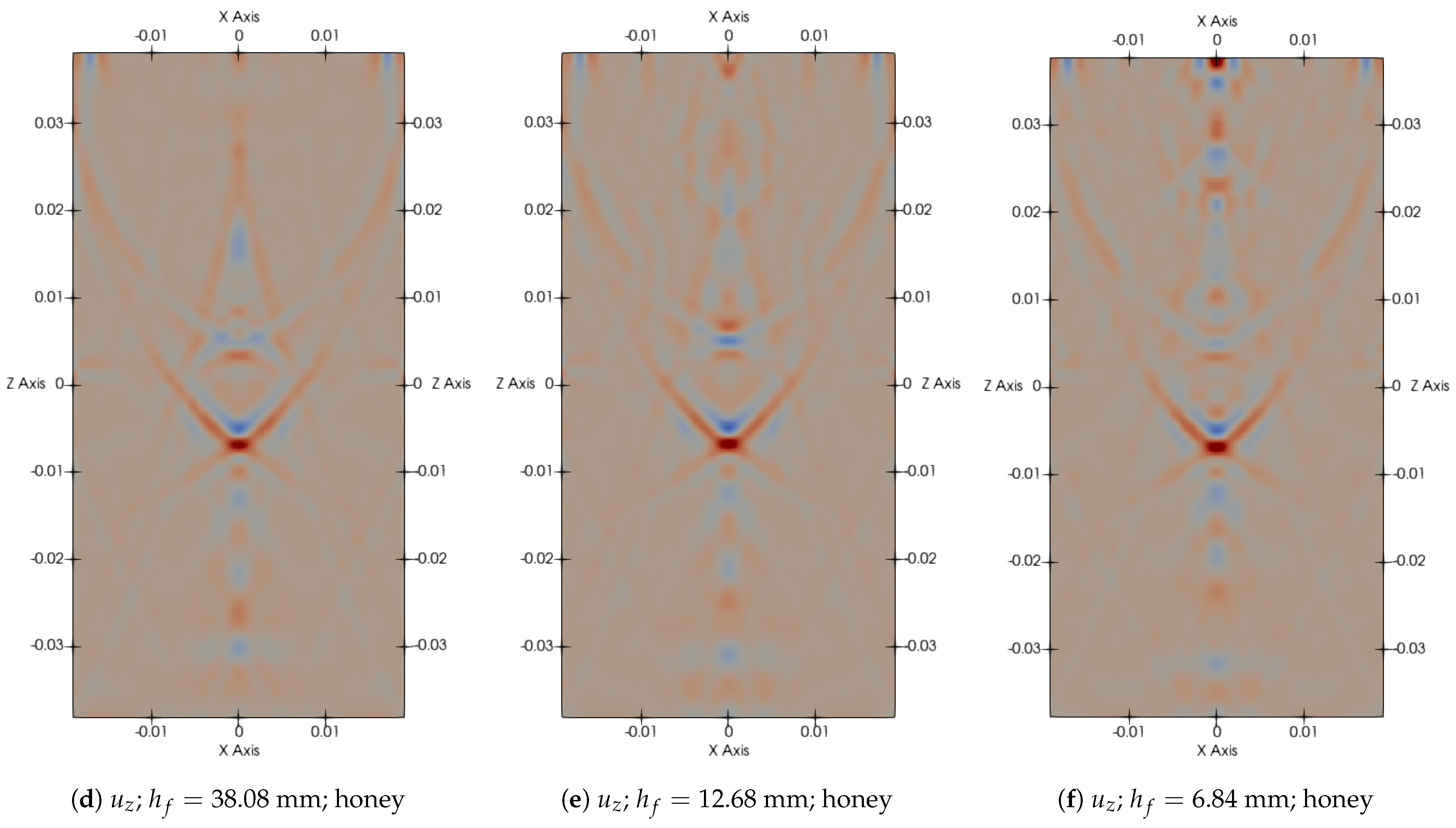
Figure 4 presents the vertical displacement field $u_z$ for three different fracture spacings with two different fluids: air (top row) and honey (bottom row). These snapshots illustrate how wave propagation is affected by both the fracture spacing and fluid type. A decrease in fracture spacing leads to more intense scattering of the wavefront. This is especially evident in the air-filled cases, where tighter spacing (Figure 4b,e) introduces interference patterns and disrupts the coherent wavefront observed at a larger fracture spacing (Figure 4a). Strong, symmetric reflections are noticeable in the air-filled cases, particularly at large fracture spacing (Figure 4a), where the high acoustic impedance contrast between the background and the low-density air results in limited wave transmission across the fractures. In contrast, the honey-filled cases show reduced reflection and smoother wavefields due to the higher density of honey, which lowers the impedance contrast and enables more effective energy transmission. As a result, wavefronts in the honey-filled models maintain greater coherency and exhibit more localized energy, with less pronounced multiple scattering.

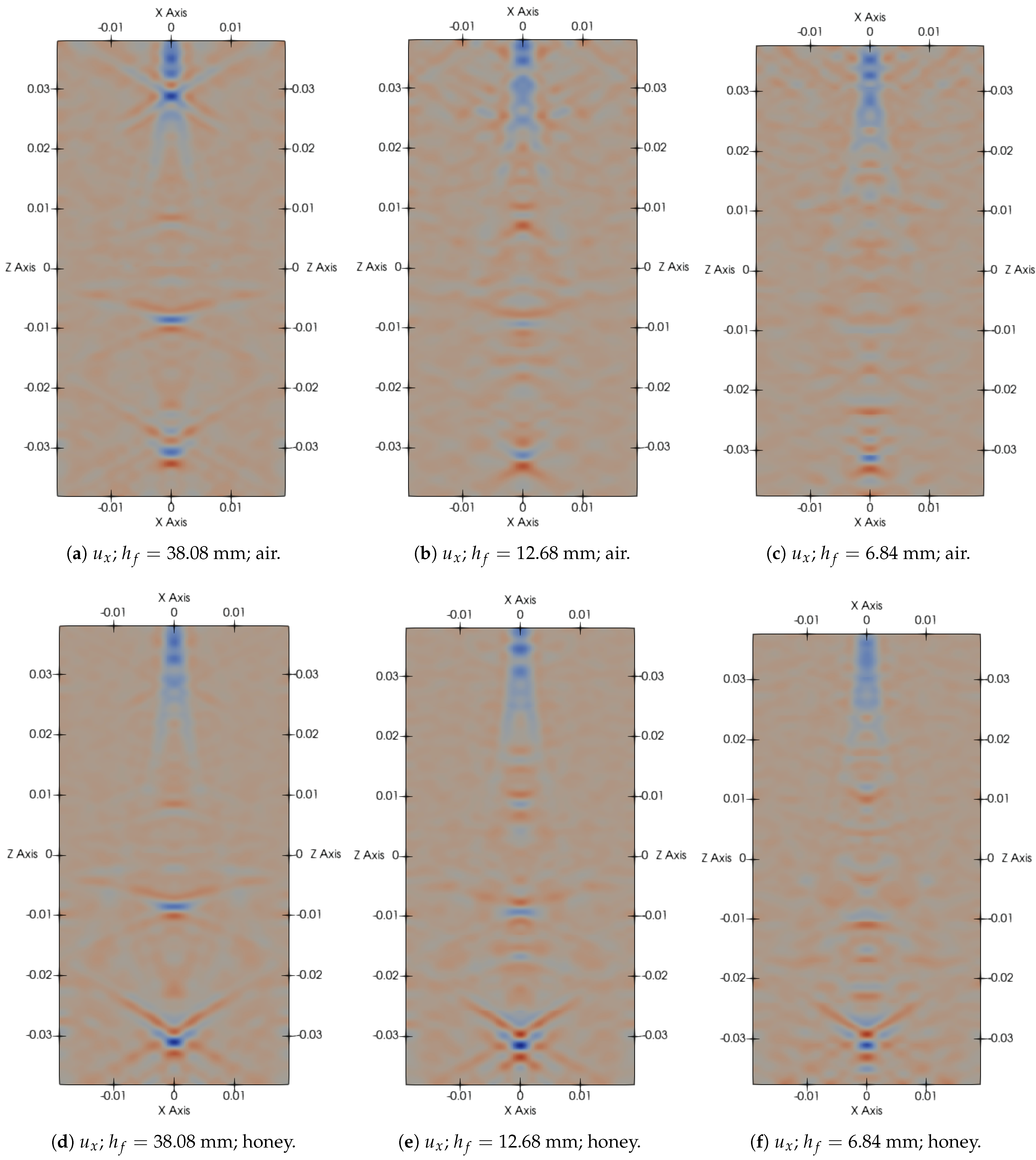
3.3.2. S-Wave Displacement Field

Figure 5 shows the horizontal displacement field $u_x$ corresponding to the S-wave propagation. Similar to the P-wave case shown in Figure 4, this figure shows results for three different fracture spacings and the same infills (air in the top row and honey in the bottom row). The displacement patterns for the S-waves are very similar between air and honey-filled fractures. The overall wavefront shapes, reflection patterns, and spatial distribution of energy remain nearly unchanged. The primary difference lies in the amplitude: in the honey-filled cases (bottom row), the displacement fields appear slightly more intense, as indicated by the stronger color saturation. As in the P-wave case, denser fluid allows better energy transmission, although for the S-wave, the effect is relatively subtle.

As fracture spacing decreases (Figure 5, left to right), the wavefields show some variation, but the wavefronts generally remain coherent and symmetric across all cases. Unlike the P-wave results, where fluid density significantly affects wave behavior, the S-wave field is less influenced by changes in fracture fill and spacing. The patterns remain highly consistent, with only subtle amplitude differences. This indicates that S-waves are less sensitive to fracture fill properties, as expected from their propagation characteristics [33].

3.4. Same Fracture Spacing with Varying Fluid

Figure 6 and Figure 7 display the vertical and horizontal displacement fields ($u_z$ and $u_x$) for a fixed fracture spacing $h_f=38.08$ mm while varying the fluid infill. The four fluids are air, water, silicon oil, and honey.

The results for vertical displacement $u_z$ (Figure 6) show that the overall wavefront becomes smoother, which means the wavefield appears more uniform, which is especially noticeable when comparing Figure 4a,c. Air-filled fractures show stronger reflections and more pronounced scattering, and fracture interfaces are more visible, while honey-filled ones exhibit less distortion. P-waves are clearly affected by the fluid type, with denser fluids promoting transmission and reducing scattering.

In contrast, the S-wavefields show less variation than P-waves, and wavefronts remain consistent across all fluid cases. There is a mild increase in amplitude saturation in the denser fluids, but the spatial patterns remain practically unchanged. The differences between the scenarios are minimal and barely distinguishable in the snapshots.

3.5. Effective Change in Wave Velocity

We conducted a more in-depth comparison of results by analyzing the seismograms recorded at the bottom of the cylinder, generated by the source at the top. Figure 8a,b show the seismograms of P- and S-waves for the three fracture spacings and different fluid types. These clearly illustrate how the presence of various fluids influences the amplitude of both P- and S-waves. Compared with the non-fractured model (black line), all fractured models (green, blue, magenta, and honey color) show a reduction in amplitude. Another notable difference is the arrival times, which vary more noticeably for P-waves. Additionally, the seismograms include multiple reflections caused by the boundary conditions and heterogeneities in the media.

The seismograms reveal that fluid type and fracture spacing affect wave propagation. Air-filled fractures (green line) exhibit the lowest amplitudes compared to viscous fluids, whereas honey preserves the highest amplitudes. These effects are more pronounced in P-waves (Figure 8a). Both P- and S-wavefronts exhibit noticeable delays inversely proportional to fluid density. This effect becomes more pronounced as fracture spacing decreases, with S-wave showing less sensitivity to these changes.

4. Discussion

Pyrak-Nolte et al. [15] conducted theoretical and experimental investigations to study wave propagation in media with multiple parallel fractures. Their experiments, conducted on laminated steel blocks, treated fractures as displacement discontinuities with specific stiffness, rather than using effective medium models. Their results demonstrated that frequency-dependent transmission coefficients, group velocity variations, and amplitude attenuation are sensitive to fracture stiffness and wave polarization. This work highlights the importance of modeling fractures explicitly. Based on this, our study uses the IP-DGM with LSM to incorporate laboratory-derived fracture compliance and fluid effects, enabling more realistic simulations of wave propagation through fluid-filled fractured media. We obtained synthetic seismograms through numerical modeling of fluid-filled fractured media. The numerical results align with the trends predicted by theoretical and analytical models.

Table 3. Comparison of laboratory and numerical P- and S-transmission coefficients for different fracture spacings and fluid types. See Ramos-Barreto et al. [28] for more details on the laboratory data.

P-Wave Transmission Coefficients
Fluid	${\mathit{h}}_{\mathit{f}}=\mathbf{38.08}$  mm		${\mathit{h}}_{\mathit{f}}=\mathbf{12.68}$  mm		${\mathit{h}}_{\mathit{f}}=\mathbf{6.84}$  mm
	Lab.	Num.	Lab.	Num.	Lab.	Num.
Air	0.37	0.32	0.02	0.03	0.00	0.01
Silicon Oil	0.89	0.89	0.69	0.62	0.34	0.30
Water	0.91	0.92	0.84	0.81	0.63	0.56
Honey	0.92	0.92	0.90	0.88	0.79	0.75
S-Wave Transmission Coefficients
Fluid	${\mathit{h}}_{\mathit{f}}=\mathbf{38.08}$  mm		${\mathit{h}}_{\mathit{f}}=\mathbf{12.68}$  mm		${\mathit{h}}_{\mathit{f}}=\mathbf{6.84}$  mm
	Lab.	Num.	Lab.	Num.	Lab.	Num.
Air	0.79	0.83	0.42	0.66	0.16	0.54
Silicon Oil	0.53	0.81	0.27	0.70	0.07	0.48
Water	0.87	0.94	0.42	0.81	0.15	0.60
Honey	0.90	0.93	0.46	0.82	0.27	0.70

presents the transmission coefficients obtained from our numerical results and those obtained from laboratory measurements by Ramos-Barreto et al. [28]. As expected, the values indicate a dependency on the fluid properties and the fracture spacing. For P-waves, transmission is highest for water and honey, particularly when fracture spacing $h_f$ is largest (fewer fractures), as indicated in the upper section of Table 3. As $h_f$ decreases (i.e., fractures are more closely spaced), transmission coefficients decrease, highlighting the effect of multiple scattering and increased wave dispersion due to more fracture interfaces. Our findings are consistent with the experimental results of Pyrak-Nolte et al. [15], who observed that group velocity and transmission coefficients depend on fracture stiffness.

A similar trend is observed for the S-wave (bottom section Table 3), where transmission is highest for the fluid-saturated cases. Contrary to common assumptions, the S-wave transmission is, in fact, comparable to or even slightly higher than the P-wave transmission in most cases. This also highlights the lower sensitivity of S-waves to fluid properties, unlike P-waves, where air-filled fractures exhibit significantly lower transmission than liquid-filled ones, the S-wave transmission coefficients remain relatively consistent across all fluids.

The decrease in transmission with decreasing fracture spacing (lower $h_f$) reinforces the experimental findings of Pyrak-Nolte et al. [15], confirming that wave velocities and transmission coefficients are significantly influenced by fracture spacing.

Moreover, the numerical results closely match those obtained from laboratory experiments (Table 3 [28]) of the wave propagation in fractured media, indicating that IP-DGM provides an accurate and reliable approach for modeling this problem.

In their study, Pyrak-Nolte et al. [15] observed that increasing the applied load on a block of steel plates increased the fracture stiffness (decreased fracture compliance), leading to higher velocities and greater wave amplitude at normal incidence. In contrast, our study varies the fluid type in the fractures. This changes the compliance and similarly influences the wave propagation, where more compliant fractures (e.g., air-filled) exhibit lower amplitudes and longer arrival times (lower velocities), while less compliant fractures (e.g., honey-filled) result in higher amplitudes and shorter arrival times.

Higher-density fluids, such as water and honey, enhance P-wave transmission compared to lower-density infills like air. This effect is attributed to the increased bulk modulus of denser fluids, which is proportional to P-wave velocity. In contrast, fluid density does not affect S-wave transmission as much. Consequently, S-wave arrival times and amplitudes show minimal variation across different fluid types. Overall, fluid density significantly influences P-wave propagation but has a minor effect on S-waves. This supports the idea that the P-wave is more sensitive to fluid properties, and the S-wave is more dependent on the solid background [33].

In our simulations, fluid properties (e.g., density) are implicitly accounted for through the fracture compliance values, reflecting the fluid-filled fracture’s mechanical response. The fluid improves coupling between fracture surfaces, facilitating better wave transmission. This behavior may be explained by the interaction between the pulse frequency (1 MHz) and the fracture thickness, where the pulse wavelength is large compared to the fracture aperture, allowing the fluid to enhance wave propagation instead of causing significant energy loss.

The validity of the numerical simulations is supported by direct comparison with laboratory measurements of P- and S-wave velocities and transmission coefficients across the range of fracture spacing and fluid types [28]. Table 3 presents a comparison of transmission coefficients. For P-wave, the numerical and laboratory results are consistent with each other, especially for water and honey, with percentage errors typically below 10%. For silicon oil, discrepancies are slightly higher (∼10–12%), while air-filled fractures show large relative differences at low transmission values due to near-zero transmission in the laboratory measurements, leading to higher percentages. In the S-waves case, the agreement is strongest at larger fracture spacings, with differences generally under 10%. At smaller fracture spacing, the model tends to overestimate transmission, particularly for fluid-filled fractures. Nonetheless, the simulations reproduce the overall trend of decreasing transmission with decreasing fracture spacing and correctly reflect the fluid-dependent behavior.

Regarding wave velocities, shown in

Table 4. Comparison of laboratory and numerical P- and S-wave velocities for different fracture spacings and fluid types. See Ramos-Barreto et al. [28] for more details on the laboratory data.

P-Wave Velocity (m/s)
Fluid	${\mathit{h}}_{\mathit{f}}=\mathbf{38}.\mathbf{08}$  mm		${\mathit{h}}_{\mathit{f}}=\mathbf{12}.\mathbf{68}$  mm		${\mathit{h}}_{\mathit{f}}=\mathbf{6}.\mathbf{84}$  mm
	Lab.	Num.	Lab.	Num.	Lab.	Num.
Air	6349	6354	6268	6021	5929	5647
Silicon Oil	6401	6387	6323	6263	6234	6056
Water	6408	6391	6366	6310	6302	6160
Honey	6416	6391	6396	6326	6362	6227
S-Wave Velocity (m/s)
Fluid	${\mathit{h}}_{\mathit{f}}=\mathbf{38}.\mathbf{08}$  mm		${\mathit{h}}_{\mathit{f}}=\mathbf{12}.\mathbf{68}$  mm		${\mathit{h}}_{\mathit{f}}=\mathbf{6}.\mathbf{84}$  mm
	Lab.	Num.	Lab.	Num.	Lab.	Num.
Air	3130	3073	3124	3059	3084	3065
Silicon Oil	3121	3070	3120	3049	3067	3035
Water	3134	3075	3127	3055	3088	3049
Honey	3136	3074	3134	3057	3119	3064

, the numerical results obtained using IP-DGM closely match the experimental data, with differences typically within 1–2% for the S-wave velocities and generally under 3% for P-waves. This close concordance demonstrates that the model not only captures the influence of fluid infill and fracture distribution but also reproduces key physical trends observed in laboratory conditions. The strong match across all tested fluids and fracture configurations reinforces the accuracy and applicability of the IP-DGM approach for simulating wave propagation in fractured media.

5. Conclusions

We simulated wave propagation across fractured media saturated with different fluids using the Interior Penalty Discontinuous Galerkin Method (IP-DGM). In this method, fractures are explicitly included without losing their discreetness. The numerical simulations of a pulse propagating across a cylinder allowed us to analyze the behavior of P- and S-waves as they travel through fractured media saturated with different fluids and evaluate how these affect the waveform.

IP-DGM effectively captures the influence of fluid type on wave propagation through compliance values. For instance, IP-DGM reproduces key wave propagation behaviors, such as reducing the amplitudes and arrival-time delays. Our results show that P-waves are more sensitive to the fluid type, with higher-density fluids enabling greater transmission and reduced wavefront distortion attributed to reduced acoustic impedance contrast. S-waves show comparatively lower sensitivity to fluid type, maintaining consistent wavefront structure and transmission across different fluid types.

Using experimentally measured compliance values strengthens the physical validity of the simulations. Our approach accurately captures the complex interplay between fluid properties and elastic wave behavior, as demonstrated by the close correspondence between numerical simulations and laboratory measurements of wave velocities and transmission coefficients across different fracture spacings and fluid types.

These results highlight the potential of IP-DGM for modeling wave propagation in complex, fractured, and fluid-saturated media and for practical applications such as seismic monitoring of fractured reservoirs. Future work could involve performing numerical simulations by scaling the compliance of the single fracture to approximate fractures of finite thickness and analyzing their impact on wave propagation.

References

1. Hall, F.; Wang, Y. Seismic response of fractures by numerical simulation. Geophys. J. Int. 2012, 189, 591–601. [Google Scholar] [CrossRef]
2. Schoenberg, M. Elastic wave behavior across linear slip interfaces. J. Acoust. Soc. Am. 1980, 68, 1516–1521. [Google Scholar] [CrossRef]
3. Hudson, J.A. Wave speeds and attenuation of elastic waves in material containing cracks. Geophys. J. Int. 1981, 64, 133–150. [Google Scholar] [CrossRef]
4. Pyrak-Nolte, L.J.; Myer, L.R.; Cook, N.G. Transmission of seismic waves across single natural fractures. J. Geophys. Res. Solid Earth 1990, 95, 8617–8638. [Google Scholar] [CrossRef]
5. Coates, R.T.; Schoenberg, M. Finite-difference modeling of faults and fractures. Geophysics 1995, 60, 1514–1526. [Google Scholar] [CrossRef]
6. Vlastos, S.; Liu, E.; Main, I.G.; Li, X.Y. Numerical simulation of wave propagation in media with discrete distributions of fractures: Effects of fracture sizes and spatial distributions. Geophys. J. Int. 2003, 152, 649–668. [Google Scholar] [CrossRef]
7. Hughes, T. The Finite Element Method. Linear Static and Dynamic Finite Element Analysis; Prentice-Hall International: Englewood Cliffs, NJ, USA, 1987. [Google Scholar]
8. Komatitsch, D.; Vilotte, J.P. The spectral element method: An efficient tool to simulate the seismic response of 2D and 3D geological structures. Bull. Seismol. Soc. Am. 1998, 88, 368–392. [Google Scholar] [CrossRef]
9. Martin, R.; Komatitsch, D.; Blitz, C.; Le Goff, N. Simulation of Seismic Wave Propagation in an Asteroid Based upon an Unstructured MPI Spectral-Element Method: Blocking and Non-blocking Communication Strategies. In High Performance Computing for Computational Science—VECPAR 2008; Palma, J.M.L.M., Amestoy, P.R., Daydé, M., Mattoso, M., Lopes, J.C., Eds.; Springer: Berlin/Heidelberg, Germany, 2008; pp. 350–363. [Google Scholar]
10. De Basabe, J.D.; Sen, M.K.; Wheeler, M.F. The interior penalty discontinuous Galerkin method for elastic wave propagation: Grid dispersion. Geophys. J. Int. 2008, 175, 83–93. [Google Scholar] [CrossRef]
11. De Basabe, J.D.; Sen, M.K.; Wheeler, M.F. Elastic wave propagation in fractured media using the discontinuous Galerkin method. Geophysics 2016, 81, T163–T174. [Google Scholar] [CrossRef]
12. Duru, K.; Rannabauer, L.; Gabriel, A.A.; Ling, O.K.A.; Igel, H.; Bader, M. A stable discontinuous Galerkin method for linear elastodynamics in 3D geometrically complex media using physics based numerical fluxes. arXiv 2019, arXiv:1907.02658. [Google Scholar]
13. Möller, T.; Friederich, W. Simulation of elastic wave propagation across fractures using a nodal discontinuous Galerkin method—theory, implementation and validation. Geophys. J. Int. 2019, 219, 1900–1914. [Google Scholar] [CrossRef]
14. Pyrak-Nolte, L.J. Fracture Specific Stiffness: The critical link between the scaling behavior of hydro-mechanical coupling in fractures and seismic monitoring. In Science of Carbon Storage in Deep Saline Formations; Elsevier: Amsterdam, The Netherlands, 2019; pp. 311–335. [Google Scholar]
15. Pyrak-Nolte, L.J.; Myer, L.R.; Cook, N.G. Anisotropy in seismic velocities and amplitudes from multiple parallel fractures. J. Geophys. Res. Solid Earth 1990, 95, 11345–11358. [Google Scholar] [CrossRef]
16. Rioyos-Romero, R. Simulación Numérica de los Efectos de las Fracturas en los Datos Sísmicos. Master’s Thesis, CICESE, Ensenada, Mexico, 2017. Available online: https://biblioteca.cicese.mx/catalogo/tesis/ficha.php?id=24798 (accessed on 5 February 2023).
17. Vamaraju, J.; Sen, M.K.; De Basabe, J.D.; Wheeler, M.F. A hybrid Galerkin finite element method for seismic wave propagation in fractured media. Geophys. J. Int. 2020, 221, 857–878. [Google Scholar] [CrossRef]
18. Zhan, Q.; Sun, Q.; Ren, Q.; Fang, Y.; Wang, H.; Liu, Q.H. A discontinuous Galerkin method for simulating the effects of arbitrary discrete fractures on elastic wave propagation. Geophys. J. Int. 2017, 210, 1219–1230. [Google Scholar] [CrossRef]
19. Gavrilieva, U.; Vasilyeva, M.; Chung, E.T. Generalized multiscale finite element method for elastic wave propagation in the frequency domain. Computation 2020, 8, 63. [Google Scholar] [CrossRef]
20. Sayers, C.M. Introduction to this special section: Fractures. Lead. Edge 2007, 26, 1102–1105. [Google Scholar] [CrossRef]
21. Hsu, C.J.; Schoenberg, M. Elastic waves through a simulated fractured medium. Geophysics 1993, 58, 964–977. [Google Scholar] [CrossRef]
22. Lubbe, R.; Worthington, M. A field investigation of fracture compliance. Geophys. Prospect. 2006, 54, 319–331. [Google Scholar] [CrossRef]
23. Lubbe, R.; Sothcott, J.; Worthington, M.; McCann, C. Laboratory estimates of normal and shear fracture compliance. Geophys. Prospect. 2008, 56, 239–247. [Google Scholar] [CrossRef]
24. Hobday, C.; Worthington, M. Field measurements of normal and shear fracture compliance. Geophys. Prospect. 2012, 60, 488–499. [Google Scholar] [CrossRef]
25. Yang, H.; Duan, H.f.; Zhu, J. Effects of filling fluid type and composition and joint orientation on acoustic wave propagation across individual fluid-filled rock joints. Int. J. Rock Mech. Min. Sci. 2020, 128, 104248. [Google Scholar] [CrossRef]
26. Möllhoff, M.; Bean, C.; Meredith, P. Rock fracture compliance derived from time delays of elastic waves. Geophys. Prospect. 2010, 58, 1111–1122. [Google Scholar] [CrossRef]
27. De Basabe, J.D.; Sen, M.K. Stability of the high-order finite elements for acoustic or elastic wave propagation with high-order time stepping. Geophys. J. Int. 2010, 181, 577–590. [Google Scholar] [CrossRef]
28. Ramos-Barreto, A.L.; Müller, T.M.; Rioyos-Romero, R.; De Basabe, J.D. Laboratory and numerical experiments of wave propagation in media with fluid-filled fractures. Wave Motion 2025. submitted. [Google Scholar]
29. The Engineering ToolBox. Air Density, Specific Weight, and Thermal Expansion Coefficients at Varying Temperatures and Pressures. 2003. Available online: https://www.engineeringtoolbox.com/water-density-specific-weight-d_595.html (accessed on 1 May 2023).
30. Gelest. Silicone Fluids Property Profile Guide. 2003. Available online: https://www.gelest.com/ (accessed on 1 May 2023).
31. The Physics Hypertextbook. Density of Water. 1998–2025. Available online: https://physics.info/density/ (accessed on 1 May 2023).
32. Faustino, C.; Pinheiro, L. Analytical rheology of honey: A state-of-the-art review. Foods 2021, 10, 1709. [Google Scholar] [CrossRef]
33. Yang, H.; Duan, H.F.; Zhu, J.; Zhao, Q. Water effects on elastic S-wave propagation and attenuation across single clay-rich rock fractures: Insights from ultrasonic measurements. Rock Mech. Rock Eng. 2024, 57, 2645–2659. [Google Scholar] [CrossRef]
Figure 1. Schematic diagram used in the numerical simulations of: (a) intact (non-fractured) model of height l = 76.08 mm and diameter d = 38 mm, and (b) a fractured model with n fractures, h f represents the fracture spacing.
Mathematics 13 01572 g001
Figure 2. Finite-element mesh created with Cubit. A wave is generated by a source at the center of the cylinder’s top surface, propagates through the medium, and is recorded by a receiver at the bottom.
Mathematics 13 01572 g002
Figure 3. Wavefield in a 3D cylindrical domain at t = 49 µs. (a) Magnitude of the displacement field for P-wave. (b) Magnitude of the displacement field for the S-wave.
Mathematics 13 01572 g003
Figure 4. Vertical displacement u z snapshots at t = 28 µs, on the x-z plane for different fracture spacing h f and fluid types. The top row corresponds to air-filled fractures, while the bottom row corresponds to honey-filled fractures. From left to right, the fracture spacing decreases.
Mathematics 13 01572 g004aMathematics 13 01572 g004b
Figure 5. Horizontal displacement u x snapshots at t = 49 µs, on the x-z plane for different fracture spacing h f and fluid types. The top row corresponds to air-filled fractures, while the bottom row corresponds to honey-filled fractures. From left to right, the fracture spacing decreases.
Mathematics 13 01572 g005
Figure 6. Displacement field u z at t = 28 µs, on the x-z plane for a fixed fracture spacing ( h f = 38.08 mm) with the four different infill fluids (a) air, (b) water, (c) silicon oil, and (d) honey.
Mathematics 13 01572 g006
Figure 7. Displacement field u x at t = 49 µs, on the x-z plane for a fixed fracture spacing ( h f = 38.08 mm) with the four different infill fluids (a) air, (b) water, (c) silicon oil, and (d) honey.
Mathematics 13 01572 g007
Figure 8. Displacement seismograms for P-waves (a) and S-waves (b) across filled fractures with varying fracture spacings and fluid type. All the amplitudes are normalized to the maximum amplitude of the non-fractured model (black line).
Mathematics 13 01572 g008