Bayesian Inference for Zero-Modified Power Series Regression Models

Abstract

Count data often exhibit discrepancies in the frequencies of zeros, which commonly occur across various application domains. These data may include excess zeros (zero inflation) or, less frequently, a scarcity of zeros (zero deflation). In regression models, both situations can arise at different levels of covariates. The zero-modified power series regression model provides an effective framework for modeling such count data, as it does not require prior knowledge of the type of zero modification, whether zero inflation or zero deflation, and can accommodate overdispersion, equidispersion, or underdispersion present in the data. This paper proposes a Bayesian estimation procedure based on the stochastic gradient Hamiltonian Monte Carlo algorithm, effectively addressing many challenges associated with estimating the model parameters. Additionally, we introduce a measure of Bayesian efficiency to evaluate the impact of prior information on parameter estimation. The practical utility of the proposed method is demonstrated through both simulated and real data across different types of zero modification.

1. Introduction

Applied statistical data analysis of count (enumeration) responses generally requires assumptions about discrete probability distributions generating the response [1,2,3,4]. In many situations, count datasets are analyzed using the Poisson distribution (see [5,6,7,8]) when we can assume that the mean and variance of the counts are the same. When the variance is assumed to be greater than or smaller than the mean, several flexible probability distributions have been proposed as alternatives to the Poisson distribution for modeling overdispersion and underdispersion [9]. They include discrete probability distributions belonging to the class of power series (PS) distributions or their generalizations [1,2,3,4,9,10,11,12].

Another often encountered situation with count data involves discrepancies in the frequency of zeros from that corresponding to the Poisson distribution. While zero inflation is most commonly observed, zero deflation can also occur in some situations. Pioneering work on these topics includes M’Kendrick [13], who studied the number of cancer cases between 1875 and 1898 in two suburbs of Luckau in Hanover, the data corresponding to a cholera epidemic in a village in India. David and Johnson [14] analyzed the number of defective teeth in 11-year-old boys and the number of ticks found on sheep. Statistical modeling of zero-inflated count data was proposed by [15,16] via the zero-inflated Poisson (ZIP) distribution, which is a mixture of a degenerate zero distribution and the Poisson distribution. For a review of ZIP models for count data, see [17]. In Dietz and Böhning [18], a zero-modified Poisson (ZMP) regression model was considered for analyzing zero-inflated or zero-deflated data. An application of the zero-inflated Poisson (ZIP) distribution for modeling data from natural calamities was presented by [19].

More recently, ref. [20] discussed zero-modified power series (ZMPS) distributions, which can adequately accommodate the discrepancy in the frequency of zeros without requiring any previous knowledge about the type of modification (zero-inflation or zero-deflation). As a special case, they illustrated the zero-modified negative binomial (ZMNB) distribution on simulated and real data, obtaining maximum likelihood estimates of model parameters. To our knowledge, the flexible and useful class of ZMPS distributions has not been employed in the literature for modeling dispersed count responses as a function of covariates, particularly in the Bayesian framework.

This paper presents a regression model for count data with the flexibility to handle different types of zero frequencies (inflation or deflation), as well as different dispersion characteristics (overdispersion or underdispersion) within a single dataset. Our framework includes, as special cases, standard regression models and zero-inflated models for count data. This paper addresses this issue in the Bayesian framework.

The sampling-based Bayesian framework using Markov Chain Monte Carlo (MCMC) methods [21] is attractive because the ZMPS likelihood function is complex, making exact Bayesian estimation and inference cumbersome. Most MCMC algorithms include an acceptance–rejection step of the generated candidate (the Metropolis–Hastings (MH) step) and may result in a high rejection rate in complex models, leading to slow convergence. To remedy this, several computationally efficient algorithms have been proposed in the literature, such as the Hamiltonian Monte Carlo (HMC) algorithm [22], the Metropolis Adjusted Langevin algorithm (MALA) [23,24,25], and an improvement of the HMC algorithm known as the No-U-Turn Sampler (NUTS) [26].

Further, the general class of algorithms using stochastic gradient MCMC (SGMCMC) [27,28,29,30,31] has gained recent popularity in the machine learning area but is still little used in the Bayesian context. An R package sgmcmc for stochastic gradient MCMC [30] calculates the gradients using a numerical computation library called tensorflow [32], which is a machine learning system with an R interface, operating on large, heterogeneous environments. In comparing algorithms in the SGMCMC class with the SGHMC algorithm, the latter is one of the most computationally efficient algorithms [31].

The objective of this paper is to develop a fully Bayesian approach for estimating the parameters of the ZMPS regression models via the computationally efficient stochastic gradient with friction HMC (SGHMC) algorithm proposed by [28]. A comprehensive study of various MCMC simulation methods is given by [33], along with a clear explanation of stochastic gradient methods. Since the required gradient equations can be obtained from the ZMPS models, we implement the SGHMC algorithm with the leapfrog integration method. We also derive and illustrate a relative Bayesian efficiency measure to compare the more general ZMPS distribution with the standard Power Series (PS) distribution.

The rest of the paper is organized as follows. Section 2.1 describes the ZMPS regression model framework for count responses. Section 2.3 presents the Bayesian approach for model parameter estimation, while Section 2.7 describes the SGHMC algorithm. Section 2.9 discusses the Bayesian information used to assess the efficiency loss incurred by fitting a ZMPS model when a PS distribution could have been applied. Section 3.1 presents simulation studies to evaluate the impact of the prior distribution on the quality of the Bayesian estimator. Section 3.2 reports the analysis of real datasets that consider different characteristics of the ZMPS distribution to analyze the number of femicides in 642 São Paulo municipalities in 2019 and 2020; in this application, we want to assess whether there was an increase in the number of femicides during the COVID-19 pandemic period. Section 4 draws some final comments on the relevant results achieved.

2. Materials and Methods

A regression model for count data is developed here, incorporating the flexibility of the ZMPS distribution, along with a Bayesian framework for parameter estimation.

2.1. ZMPS Regression Model

In ZMPS regression, suppose that the observations to be analyzed are represented by the vector $\mathit{y}={(y_1,\dots ,y_n)}^{\prime }$. Let $Y_i$, $i=1\dots n$ be n independent random variables assuming values in the support set $\mathcal{A}=\{0,1,\dots \}$ and having probability mass function (p.m.f.) defined by  [20]

$${\pi }_{ZMPS}(y_i;{\mu }_i,\varphi ,p_i)=(1-p_i)I\left(y_i\right)+p_i{\pi }_{PS}(y_i;{\mu }_i,\varphi ),$$

(1)

where ${\mu }_i>0$, $\varphi >0$, and the indicator function $I\left(y_i\right)=1$ if $y_i=0$ and $I\left(y_i\right)=0$ if $y_i>0$. The p.m.f. of the standard PS distribution is given by

$${\pi }_{PS}(y_i;{\mu }_i,\varphi )={\displaystyle \frac{a(y_i,\varphi ){\left(g({\mu }_i,\varphi )\right)}^{y_i}}{f({\mu }_i,\varphi )}},$$

where $a(y_i,\varphi )$, $f({\mu }_i,\varphi )$ and $g({\mu }_i,\varphi )$ are positive, finite, and twice-differentiable functions, with ${\displaystyle f({\mu }_i,\varphi )=\sum _{y_i\in {\mathcal{A}}_0}a(y_i,\varphi )g{({\mu }_i,\varphi )}^{y_i}}$, while the parameter $p_i$ is responsible for modifying the probability of zero of the standard PS distribution, such that

$$0\le p_i\le {\displaystyle \frac{1}{1-{\pi }_{PS}(0;{\mu }_i,\varphi )}},$$

where ${\pi }_{PS}(0;{\mu }_i,\varphi )$ is the probability of zero in the PS distribution.

The Poisson, generalized Poisson, COM-Poisson, and negative binomial distributions are well-known members of the PS family.

Table 1. Distributions within the PS family.

PS	Distribution	$\mathit{f}({\mathit{\mu }}_{\mathit{i}},\mathit{\varphi })$	$\mathit{g}({\mathit{\mu }}_{\mathit{i}},\mathit{\varphi })$	$\mathit{a}({\mathit{y}}_{\mathit{i}},\mathit{\varphi })$
P	Poisson	$e^{{\mu }_i}$	${\mu }_i$	${\displaystyle \frac{1}{y_i!}}$
GP	Generalized	$e^{{\mu }_i{(1+{\mu }_i\varphi )}^{-1}}$	${\displaystyle \frac{{\mu }_i{e}^{-{\mu }_i\varphi {(1+{\mu }_i\varphi )}^{-1}}}{1+{\mu }_i\varphi }}$	${\displaystyle \frac{{(1+\varphi y_i)}^{y_i-1}}{y_i!}}$
	Poisson
COMP	COM-Poisson	${\displaystyle \sum _{s=0}^{\infty }{\left({\displaystyle \frac{{\mu }_i^s}{s!}}\right)}^{\varphi }}$	${\mu }_i^{\varphi }$	${\left({\displaystyle \frac{1}{y_i!}}\right)}^{\varphi }$
NB	Negative	${\left({\displaystyle \frac{\varphi }{{\mu }_i+\varphi }}\right)}^{-\varphi }$	${\displaystyle \frac{{\mu }_i}{{\mu }_i+\varphi }}$	${\displaystyle \frac{\Gamma (\varphi +y_i)}{y_i!\Gamma \left(\varphi \right)}}$
	Binomial

presents the functions $f({\mu }_i,\varphi )$, $g({\mu }_i,\varphi )$, and $a(y_i,\varphi )$ for several distributions within the PS family.

For the COM-Poisson distribution, we consider the parameterization proposed in [34] to provide a clearly centering parameter. The conditional mean and variance of $Y_i$, $E\left(Y_i\right)={\mu }_i^{PS}$ and $V\left(Y_i\right)={\upsilon }_i^{PS}$, are given by

$${\mu }_i^{PS}={\displaystyle \frac{f_{\mu }({\mu }_i,\varphi )g({\mu }_i,\varphi )}{f({\mu }_i,\varphi )g_{\mu }({\mu }_i,\varphi )}}\mathrm{and}{\upsilon }_i^{PS}={\displaystyle \frac{g({\mu }_i,\varphi )}{g_{\mu }({\mu }_i,\varphi )}},$$

where $f_{\mu }$ and $g_{\mu }$ denote derivatives with respect to $\mu$. For the distributions shown in Table 1, the mean ${\mu }_i^{PS}={\mu }_i$, except for the COM-Poisson distribution, for which we can write the asymptotic approximations [34]:

$${\mu }_i^{PS}\approx {\mu }_i+{\displaystyle \frac{1-\varphi }{2\varphi }}\mathrm{and}{\upsilon }_i^{PS}\approx {\displaystyle \frac{{\mu }_i}{\varphi }}.$$

This parametrization also allows $\varphi$ to keep its role as a shape parameter. That is, if $\varphi <1$, the variance is greater than the mean (overdispersion), while $\varphi >1$ leads to underdispersion. The mean and variance of random variable $Y_i$ are, respectively,

$${\mu }_i^{\left(ZMPS\right)}=p_i{\mu }_i^{PS}\mathrm{and}{\sigma }_i^{2\left(ZMPS\right)}=p_i\{{\upsilon }_i^{PS}+(1-p_i){\left({\mu }_i^{PS}\right)}^2\},$$

Different values of $p_i$ lead to different ZMPS distributions, as can be seen in the evaluation of the proportion of additional or missing zeros, given by

$$\begin{array}{ccc}\hfill {\pi }_{ZMPS}(0;{\mu }_i,\varphi ,p_i)-{\pi }_{PS}(0;{\mu }_i,\varphi )& =& 1-p_i+p_i{\pi }_{PS}(0;{\mu }_i,\varphi )-{\pi }_{PS}(0;{\mu }_i,\varphi )\hfill \\ & =& (1-p_i)(1-{\pi }_{PS}(0;{\mu }_i,\varphi )).\hfill \end{array}$$

(2)

According to (2), parameter $p_i$ also controls the frequency of zeros, such as the following:

(i)

When $p_i=0$ in (2), ${\pi }_{ZMPS}(0;{\mu }_i,\varphi ,p_i)=1$, and (1) is the degenerate distribution with the entire mass at zero.

(ii)

For all $0<p_i<1$ in (2), $(1-p_i)(1-{\pi }_{PS}(0;{\mu }_i,\varphi ))>0$. Then, ${\pi }_{ZMPS}(0;{\mu }_i,\varphi ,p_i)>{\pi }_{PS}(0;{\mu }_i,\varphi )$, and (1) is the zero-inflated PS (ZIPS) distribution, which has a proportion of additional zeros.

(iii)

When $p_i=1$ in (2), ${\pi }_{ZMPS}(0;{\mu }_i,\varphi ,p_i)-{\pi }_{PS}(0;{\mu }_i,\varphi )=0$. Therefore, ${\pi }_{ZMPS}(0;{\mu }_i,\varphi ,p_i)={\pi }_{PS}(0;{\mu }_i,\varphi )$, and (1) is the standard PS distribution.

(iv)

For all $1<p_i<{\displaystyle \frac{1}{1-{\pi }_{PS}(0;{\mu }_i,\varphi )}}$ in (2), $(1-p_i)(1-{\pi }_{PS}(0;{\mu }_i,\varphi ))<0$. Then, ${\pi }_{ZMPS}(0;{\mu }_i,\varphi ,p_i)$$<{\pi }_{PS}(0;{\mu }_i,\varphi )$, and (1) is the zero-deflated negative binomial (ZDPS) distribution.

(v)

When $p_i={\displaystyle \frac{1}{1-{\pi }_{PS}(0;{\mu }_i,\varphi )}}$ in (2), ${\pi }_{ZMPS}(0;{\mu }_i,\varphi ,p_i)=0$. Then, (1) is the zero-truncated PS (ZTPS) distribution, whose p.m.f. is given by

$$\begin{array}{c}\hfill {\pi }_{ZTPS}(y_i;{\mu }_i,\varphi )={\displaystyle \frac{{\pi }_{PS}(y_i;{\mu }_i,\varphi )}{1-{\pi }_{PS}(0;{\mu }_i,\varphi )}}(1-I\left(y_i\right)),y_i\in \mathcal{A}.\end{array}$$

(3)

Note that the parameter $p_i$ controls the frequency of zeros and can assume different values at specific levels of covariates. Conditions (i)–(v) indicate that in zero inflation count data, deflation or standard zero frequency may occur in the same dataset at specific levels of covariates. Therefore, it is plausible that the ZMPS model can model these situations by considering different values of $p_i$. More details about the ZMPS distributions are provided in Conceiçao et al. [20].

2.2. Hurdle Model Versus ZMPS Model

Note that (1) can be rewritten as

$$\begin{array}{ccc}\hfill {\pi }_{ZMPS}(y_i;{\mu }_i,\varphi ,p_i)& =& {\pi }_{ZMPS}(0;{\mu }_i,\varphi ,p_i)I\left(y_i\right)+{\pi }_{ZMPS}(y_i;{\mu }_i,\varphi ,p_i)(1-I\left(y_i\right))\hfill \\ \hfill & =& \{1-p_i+p_i{\pi }_{PS}(0;{\mu }_i,\varphi ))\}I\left(y_i\right)+\left\{p_i{\pi }_{PS}(y_i;{\mu }_i,\varphi )\right\}(1-I\left(y_i\right))\hfill \\ \hfill & =& \{1-p_i(1-{\pi }_{PS}(0;{\mu }_i,\varphi ))\}I\left(y_i\right)+\hfill \\ & & p_i(1-{\pi }_{PS}(0;{\mu }_i,\varphi ))\left\{{\displaystyle \frac{{\pi }_{PS}(y_i;{\mu }_i,\varphi )}{1-{\pi }_{PS}(0;{\mu }_i,\varphi )}}(1-I\left(y_i\right))\right\}.\hfill \end{array}$$

(4)

Since $0\le p_i\le {\displaystyle \frac{1}{1-{\pi }_{PS}(0;{\mu }_i,\varphi )}}$, then $0\le p_i(1-{\pi }_{PS}(0;{\mu }_i,\varphi ))\le 1$. Thus, setting ${\omega }_i=p_i(1-{\pi }_{PS}(0;{\mu }_i,\varphi ))$, the p.m.f. given in (4) can be written as a mixture distribution, i.e.,

$${\pi }_{ZMPS}(y_i;{\mu }_i,\varphi ,{\omega }_i)=(1-{\omega }_i)I\left(y_i\right)+{\omega }_i{\pi }_{ZTPS}(y_i;{\mu }_i,\varphi ),y_i\in \mathcal{A},$$

(5)

where $0\le {\omega }_i\le 1$

The ZMPS distribution in (5) is parameterized by ${\omega }_i$ and can be interpreted as a hurdle distribution [35], where the probability of the event $Y_i=0$ is $1-{\omega }_i$, while the probability of an observation $Y_i=y_i$, $y_i>0$ is ${\omega }_i{\pi }_{ZTPS}(y_i;{\mu }_i,\varphi )$.

Properties (i)–(v) can also be written in terms of ${\omega }_i$. Therefore, the ZMPS model (1) and the hurdle model (5) are equivalent, and either can be used to model data with zero-frequency modifications (inflation or deflation). Ref. [36] compared the hurdle model to zero-inflated models, highlighting the advantages of hurdle models (or ZMPS) due to the viability of these models to consider zero-inflation $(0<p_i<1)$ and zero-deflation $(1<p_i\le 1/(1-{\pi }_{PS}(0;{\mu }_i,\varphi )))$ with different levels of covariates. Henceforth, we will consider the hurdle version of ZMPS given by (5).

However, it is essential to note that ZMPS models may have a drawback when $p_i=1$ for all $i=1,\dots ,n$. A standard PS model could have been used without fitting the parameters $p_i$. We can only say that fitting a ZMPS model instead of a simple PS model in this scenario may result in efficiency losses for the parameter estimators. This paper offers a method to assess this efficiency loss from a Bayesian perspective (see Section 2.9).

Let ${\mathit{x}}_i={(x_{i,1},\dots ,x_{i,r})}^{\prime }$ with $x_{i,1}=1$, and ${\mathit{v}}_i={(v_{i,1},\dots ,v_{i,s})}^{\prime }$, with $v_{i,1}=1$, be fixed predictors. Let $\mathit{X}={({\mathit{x}}_1^{\prime },\dots ,{\mathit{x}}_n^{\prime })}^{\prime }$ and $\mathit{V}={({\mathit{v}}_1^{\prime },\dots ,{\mathit{v}}_n^{\prime })}^{\prime }$, respectively, denote the $n\times r$ and $n\times s$ predictor matrices employed for modeling the ${\mu }_i$ and ${\omega }_i$, respectively, via the dual-link function given by logarithmic and logit link functions, i.e.,

$$\begin{array}{cc}\hfill log\left({\mu }_i\right)& ={\eta }_1({\mathit{\beta }}_{\mu },{\mathit{x}}_i)={\beta }_{\mu ,1}+\sum _{j=2}^r{\beta }_{\mu ,j}{x}_{i,j},\hfill \\ \hfill \mathrm{logit}\left({\omega }_i\right)& ={\eta }_2({\mathit{\beta }}_{\omega },{\mathit{v}}_i)={\beta }_{\omega ,1}+\sum _{j=2}^s{\beta }_{\omega ,j}{v}_{i,j}.\hfill \end{array}$$

where ${\mathit{\beta }}_{\mu }={({\beta }_{\mu ,1}\dots {\beta }_{\mu ,r})}^{\prime }$, ${\mathit{\beta }}_{\omega }={({\beta }_{\omega ,1}\dots ,{\beta }_{\omega ,s})}^{\prime }$. It is also possible to employ alternate link functions for ${\omega }_i$; see [37].

The parameter $\varphi$ accounts for under- or overdispersion in the data, in addition to any dispersion caused by zero inflation or zero deflation. In the case of the zero-modified Poisson distribution, $\varphi =1$, and all the overdispersion is attributed to zero inflation. In other models, some of the under- or overdispersion is explained by the parameters ${\omega }_i$ and ${\mu }_i$. Therefore, we interpret $\varphi$ as capturing any under- or overdispersion beyond that induced by zero-modification, without the need for additional covariates.

2.3. Bayesian Framework for the ZMPS Regression Model

Let $\mathcal{D}=\{\mathit{y},\mathit{X},\mathit{V}\}$ denote the observed data, based on which we estimate the parameters ${\mathit{\beta }}_{\mu }^{\prime },{\mathit{\beta }}_{\omega }^{\prime },\varphi$ under the model in (5) using the fully Bayesian framework.

2.4. Likelihood Function

The likelihood function is

$${\displaystyle \mathcal{L}({\mathit{\beta }}_{\mu },{\mathit{\beta }}_{\omega },\varphi |\mathcal{D})=\prod _{i=1}^n{\left(1-{\omega }_i\right)}^{I\left(y_i\right)}{\left({\omega }_i{\pi }_{ZTPS}(y_i;{\mu }_i,\varphi )\right)}^{(1-I\left(y_i\right))},}$$

(6)

where ${\mu }_i>0$ and $0<{\omega }_i<1$. It follows that the log-likelihood function is

$$\begin{array}{ccc}\hfill \mathsf{\ell }({\mathit{\beta }}_{\mu },{\mathit{\beta }}_{\omega },\varphi \mid \mathcal{D})& =& \sum _{i=1}^{n}I\left(y_i\right)log(1-{\omega }_i)+\left(1-I\left(y_i\right)\right)log\left({\omega }_i{\pi }_{ZTPS}(y_i\mid {\mu }_i,\varphi )\right),\hfill \\ \hfill & =& \sum _{i=i}^n\left\{I\left(y_i\right)log\left({\displaystyle \frac{1-{\omega }_i}{{\omega }_i}}\right)+log\left({\omega }_i\right)\right\}+\hfill \\ \hfill & & \sum _{i=1}^n\left(1-I\left(y_i\right)\right)log\left({\pi }_{ZTPS}(y_i\mid {\mu }_i,\varphi )\right)\hfill \\ \hfill & =& {\mathsf{\ell }}_1({\mathit{\beta }}_{\mu },\varphi \mid \mathcal{D})+{\mathsf{\ell }}_2({\mathit{\beta }}_{\omega }\mid \mathcal{D}),\hfill \end{array}$$

where

$${\mathsf{\ell }}_1({\mathit{\beta }}_{\mu },\varphi \mid \mathcal{D})=\sum _{i=1}^n\left(1-I\left(y_i\right)\right)log\left({\pi }_{ZTPS}(y_i\mid {\mu }_i,\varphi ,\mathcal{D})\right)$$

(7)

and

$${\mathsf{\ell }}_2({\mathit{\beta }}_{\omega }\mid \mathcal{D})=\sum _{i=1}^{n}I\left(y_i\right)log\left({\displaystyle \frac{1-{\omega }_i}{{\omega }_i}}\right)+log\left({\omega }_i\right).$$

(8)

Here, ${\mathsf{\ell }}_1({\mathit{\beta }}_{\mu },\varphi \mid \mathcal{D})$ is the portion of the log-likelihood function from the associated ZTPS distribution, considering only the positive observations of $\mathit{y}$, and ${\mathsf{\ell }}_2({\mathit{\beta }}_{\omega }\mid \mathcal{D})$ is the part associated with the hurdle parameter ${\mathit{\beta }}_{\omega }$. Therefore, we can estimate the parameters ${\mathit{\beta }}_{\mu }$ and $\varphi$ of the ZMPS distribution from its associated ZTPS distribution using only the positive observations of the sample $\mathbf{y}$. The following result states a relevant link between the estimation of the parameters of ZMPS and ZTPS distributions.

Result 1.

If $Y_i$ follows the ZMPS distribution, we can estimate the ${\mathit{\beta }}_{\mu }$ and $\varphi$ parameters by only considering the positive observations of $\mathit{y}$ and the associated ZTPS distribution.

To verify this result, let ${\mathit{y}}^{+}={(y_1^{+},\dots ,y_m^{+})}^{\prime }$ denote the positive observations in $\mathit{y}$, where $m=n-n_0$, and $n_0$ is the number of zero observations in the vector $\mathit{y}$. Let ${\mathit{X}}^{+}$ denote the $m\times r$ predictor matrix associated with ${\mathit{y}}^{+}$. Assuming that ${\mathit{y}}^{+}$ follows the associated ZTPS distribution and ${\mathcal{D}}^{+}=({\mathit{y}}^{+},{\mathit{X}}^{+})$, the log-likelihood function associated with ${\mathit{y}}^{+}$ is given by

$${\mathsf{\ell }}_{ZTPS}({\mathit{\beta }}_{\mu },\varphi \mid {\mathcal{D}}^{+})=\sum _{i=1}^{m}log\left({\pi }_{ZTPS}(y_i^{+}\mid {\mu }_i,\varphi ,{\mathcal{D}}^{+})\right).$$

(9)

We can easily show that (9) is obtained directly from (7). We see from (7) and (8) that estimation of (${\mathit{\beta }}_{\mu },\varphi$) independently of the parameter is independent of estimating ${\mathit{\beta }}_{\omega }$. Substituting

$${\pi }_{ZTPS}(y_i^{+}\mid {\mu }_i,\varphi )={\displaystyle \frac{a(y_i^{+},\varphi )g{({\mu }_i,\varphi )}^{y_i^{+}}}{f({\mu }_i,\varphi )-1}},y_i^{+}\in \{1,2,\dots \}$$

in (9) and differentiating ${\mathsf{\ell }}_{ZTPS}({\mathit{\beta }}_{\mathit{\mu }},\varphi \mid {\mathcal{D}}^{+})$ with respect to each parameter, ${\mathit{\beta }}_{\mu ,j}$, $j=1,\dots r$, and $\varphi$, we obtain the score vectors ${\mathcal{U}}_{{\mathit{\beta }}_{\mu }}$ and ${\mathcal{U}}_{\varphi }$ with elements:

$${\mathcal{U}}_{{\beta }_{\mu ,j}}={\displaystyle \frac{\partial {\mathsf{\ell }}_{ZTPS}({\mathit{\beta }}_{\mu },\varphi \mid {\mathcal{D}}^{+})}{\partial {\beta }_{\mu ,j}}}=\sum _{i=1}^m\left[y_i^{+}{\displaystyle \frac{g_{\mu }({\mu }_i,\varphi )}{g({\mu }_i,\varphi )}}-{\displaystyle \frac{f_{\mu }({\mu }_i,\varphi )}{f({\mu }_i,\varphi )-1}}\right]{\displaystyle \frac{\partial {\mu }_i}{\partial {\beta }_{\mu ,j}}}$$

and

$${\mathcal{U}}_{\varphi }={\displaystyle \frac{\partial {\mathsf{\ell }}_{ZTPS}({\mathit{\beta }}_{\mu },\varphi \mid {\mathcal{D}}^{+})}{\partial \varphi }}=\sum _{i=1}^m\left[{\displaystyle \frac{a_{\varphi }(y_i^{+},\varphi )}{a(y_i,\varphi )}}+y_i^{+}{\displaystyle \frac{g_{\varphi }({\mu }_i,\varphi )}{g({\mu }_i,\varphi )}}-{\displaystyle \frac{f_{\varphi }({\mu }_i,\varphi )}{f({\mu }_i,\varphi )-1}}\right],$$

where

$g_{\mu }({\mu }_i,\varphi )=\partial g({\mu }_i,\varphi )/\partial {\mu }_i$, $f_{\mu }=\partial f({\mu }_i,\varphi )/\partial {\mu }_i$, $a_{\varphi }=\partial a(y_i,\varphi )/\partial \varphi$, $g_{\varphi }=\partial g({\mu }_i,\varphi )/\partial \varphi$, and $f_{\varphi }=\partial f({\mu }_i,\varphi )/\partial \varphi$. Considering the logit link function $\mathrm{logit}\left({\omega }_i\right)=log\left({\omega }_i/(1-{\omega }_i)\right)={\mathit{v}}_i^{\prime }{\mathit{\beta }}_{\omega }$ and differentiating ${\mathsf{\ell }}_2({\mathit{\beta }}_{\omega }\mid \mathcal{D})$ with respect to each parameter, ${\mathit{\beta }}_{\omega ,j}$, $j=1,\dots s$, we obtain the score vector ${\mathcal{U}}_{{\mathit{\beta }}_{\omega }}$, whose elements are

$${\mathcal{U}}_{{\beta }_{\omega ,j}}={\displaystyle \frac{\partial {\mathsf{\ell }}_2({\mathit{\beta }}_{\omega }\mid \mathcal{D})}{\partial {\beta }_{\omega ,j}}}=\sum _{i=1}^n\left(1-I\left(y_i\right)\right)v_{i,j}-\left({\displaystyle \frac{e^{{\mathit{v}}_i^{\prime }{\mathit{\beta }}_{\omega }}}{1+e^{{\mathit{v}}_i^{\prime }{\mathit{\beta }}_{\omega }}}}\right)v_{i,j}.$$

The score vector, denoted by $\mathcal{U}({\mathit{\beta }}_{\mu },\varphi ,{\mathit{\beta }}_{\omega })={({\mathcal{U}}_{{\mathit{\beta }}_{\mu }}({\mathit{\beta }}_{\mu },\varphi ),{\mathcal{U}}_{\varphi }({\mathit{\beta }}_{\mu },\varphi ),{\mathcal{U}}_{{\mathit{\beta }}_{\omega }}\left({\mathit{\beta }}_{\omega }\right))}^{\prime }$, will play a role in the MCMC simulation algorithm in the Bayesian approach.

Let the parameter vector be denoted by $\mathit{\theta }={({\mathit{\beta }}_{\mu }^{\prime },{\mathit{\beta }}_{\omega }^{\prime },\varphi )}^{\prime }$, where $\mathit{\theta }={({\theta }_1,\dots ,{\theta }_m)}^{\prime }$ and $m=r+s+1$. The observed information matrix $\mathcal{J}\left(\mathit{\theta }\right)$ is an $(r+s+1)\times (r+s+1)$ matrix, with entries given by

$${\mathcal{J}}_{j,k}=-{\displaystyle \frac{{\partial }^{2}log\mathcal{L}(\mathit{\theta }\mid \mathcal{D})}{\partial {\theta }_j\partial {\theta }_k}},j,k=1,\dots ,(r+s+1).$$

Due to the orthogonality between the parameters $({\mathit{\beta }}_{\mu },\varphi )$ and ${\mathit{\beta }}_{\omega }$, the information matrix $\mathcal{J}\left(\mathit{\theta }\right)$ is a block diagonal matrix given by

$$\mathcal{J}\left(\mathit{\theta }\right)=\left[\begin{array}{ccc}{\mathcal{J}}_{{\mathit{\beta }}_{\mu },{\mathit{\beta }}_{\mu }}& {\mathcal{J}}_{{\mathit{\beta }}_{\mu },\varphi }& \mathbf{0}\\ {\mathcal{J}}_{{\mathit{\beta }}_{\mu },\varphi }^{\prime }& {\mathcal{J}}_{\varphi ,\varphi }& \mathbf{0}\\ \mathbf{0}& \mathbf{0}& {\mathcal{J}}_{{\mathit{\beta }}_{\omega },{\mathit{\beta }}_{\omega }}\end{array}\right].$$

(10)

The elements of each block are defined by

$$\begin{array}{ccc}\hfill {\mathcal{J}}_{{\mathit{\beta }}_{\mu j},{\mathit{\beta }}_{\mu k}}& =& -{\displaystyle \frac{{\partial }^2{\mathsf{\ell }}_{ZTPS}({\mathit{\beta }}_{\mu },\varphi |{\mathcal{D}}^{+})}{\partial {\mathit{\beta }}_{\mu }\partial {\mathit{\beta }}_{\mu }^{\prime }}}\hfill \\ & =& \sum _{i=1}^m\left[-y_i^{+}{h}_g({\mathit{\beta }}_{\mu },\varphi )+h_f({\mathit{\beta }}_{\mu },\varphi )\right]\left({\displaystyle \frac{\partial {\mu }_i}{\partial {\beta }_{\mu ,j}}}\right)\left({\displaystyle \frac{\partial {\mu }_i}{\partial {\beta }_{\mu ,k}}}\right)-\hfill \\ & & \sum _{i=1}^m\left[y_i^{+}{\displaystyle \frac{g_{\mu }({\mu }_i,\varphi )}{g({\mu }_i,\varphi )}}-{\displaystyle \frac{f_{\mu }({\mu }_i,\varphi )}{f({\mu }_i,\varphi )-1}}\right]\left({\displaystyle \frac{{\partial }^2{\mu }_i}{\partial {\beta }_{\mu ,j}\partial {\beta }_{\mu ,k}}}\right),\hfill \end{array}$$

$$\begin{array}{ccc}\hfill {\mathcal{J}}_{{\mathit{\beta }}_{\mu },\varphi }& =& {\mathcal{J}}_{\varphi ,{\mathit{\beta }}_{\mu }}=-{\displaystyle \frac{{\partial }^2{\mathsf{\ell }}_{ZTPS}({\mathit{\beta }}_{\mu },\varphi |{\mathcal{D}}^{+})}{\partial \varphi \partial {\mathit{\beta }}_{\mu }}}\hfill \\ & =& \sum _{i=1}^m\left[-y_i^{+}{t}_g({\mathit{\beta }}_{\mu },\varphi )+t_f({\mathit{\beta }}_{\mu },\varphi )\right]\left({\displaystyle \frac{\partial {\mu }_i}{\partial {\beta }_{\mu ,j}}}\right),\hfill \end{array}$$

$$\begin{array}{ccc}\hfill {\mathcal{J}}_{\varphi ,\varphi }& =& -{\displaystyle \frac{{\partial }^2{\mathsf{\ell }}_{ZTPS}({\mathit{\beta }}_{\mu },\varphi |{\mathcal{D}}^{+})}{\partial {\varphi }^2}}\hfill \\ & =& \sum _{i=1}^m\left[-k_a(y_i^{+},\varphi )-y_i^{+}{k}_g({\mathit{\beta }}_{\mu },\varphi )+k_f({\mathit{\beta }}_{\mu },\varphi )\right],\hfill \\ \hfill {\mathcal{J}}_{{\beta }_{\omega j},{\beta }_{\omega k}}& =& -{\displaystyle \frac{{\partial }^2{\mathsf{\ell }}_2\left({\mathit{\beta }}_{\omega }\right|\mathcal{D})}{\partial {\mathit{\beta }}_{\omega }\partial {\mathit{\beta }}_{\omega }^{\prime }}}=\sum _{i=1}^n{\displaystyle \frac{{\mathit{x}}_i^{\prime }{\mathit{x}}_k{\omega }_i}{1-e^{{\mathit{x}}_i^{\prime }{\mathit{\beta }}_{\omega }}}},\hfill \end{array}$$

where

$$\begin{array}{ccc}\hfill h_g({\mathit{\beta }}_{\mu },\varphi )& =& {\displaystyle \frac{g_{\mu \mu }({\mu }_i,\varphi )g({\mu }_i,\varphi )-g_{\mu }^2({\mu }_i,\varphi )}{g{({\mu }_i,\varphi )}^2}},\hfill \\ \hfill h_f({\mathit{\beta }}_{\mu },\varphi )& =& {\displaystyle \frac{f_{\mu \mu }({\mu }_i,\varphi )(f({\mu }_i,\varphi )-1)-f_{{\mu }_i}^2({\mu }_i,\varphi )}{{(f({\mu }_i,\varphi )-1)}^2}},\hfill \\ \hfill k_a(y_i^{+},\varphi )& =& {\displaystyle \frac{a_{\varphi \varphi }(y_i^{+},\varphi )a(y_i^{+},\varphi )-a_{\varphi }^2(y_i^{+},\varphi )}{a{(y_i^{+},\varphi )}^2}},\hfill \\ \hfill k_g({\mathit{\beta }}_{\mu },\varphi )& =& {\displaystyle \frac{g_{\varphi \varphi }({\mu }_i,\varphi )g({\mu }_i,\varphi )-g_{\varphi }^2({\mu }_i,\varphi )}{g{({\mu }_i,\varphi )}^2}},\hfill \\ \hfill k_f({\mathit{\beta }}_{\mu },\varphi )& =& {\displaystyle \frac{f_{\varphi \varphi }({\mu }_i,\varphi )(f({\mu }_i,\varphi )-1)-f_{\varphi }^2({\mu }_i,\varphi )}{{(f({\mu }_i,\varphi )-1)}^2}},\hfill \\ \hfill t_g({\mathit{\beta }}_{\mu },\varphi )& =& {\displaystyle \frac{g_{\mu \varphi }({\mu }_i,\varphi )g({\mu }_i,\varphi )-g_{\mu }({\mu }_i,\varphi )g_{\varphi }({\mu }_i,\varphi )}{g{({\mu }_i,\varphi )}^2}},\hfill \\ \hfill t_f({\mathit{\beta }}_{\mu },\varphi )& =& {\displaystyle \frac{f_{\mu \varphi }({\mu }_i,\varphi )(f({\mu }_i,\varphi )-1)-f_{\mu }({\mu }_i,\varphi )f_{\varphi }({\mu }_i,\varphi )}{{(f({\mu }_i,\varphi )-1)}^2}},\hfill \end{array}$$

and, $g_{\mu \mu }({\mu }_i,\varphi )={\partial }^{2}g({\mu }_i,\varphi )/\partial {\mu }_i^2$, $f_{\mu \mu }={\partial }^{2}f({\mu }_i,\varphi )/\partial {\mu }_i^2$, $a_{\varphi \varphi }={\partial }^{2}a(y_i,\varphi )/\partial {\varphi }^2$, $g_{\varphi \varphi }={\partial }^{2}g({\mu }_i,\varphi )/\partial {\varphi }^2$, and $f_{\varphi \varphi }={\partial }^{2}f({\mu }_i,\varphi )/\partial {\varphi }^2$, $g_{\mu \varphi }({\mu }_i,\varphi )={\partial }^{2}g({\mu }_i,\varphi )/\partial {\mu }_i\partial \varphi$, $f_{\mu \varphi }={\partial }^{2}f({\mu }_i,\varphi )/\partial {\mu }_i\partial \varphi$.

2.5. Prior Distributions

Assuming prior independence, we have ${\pi }_0({\mathit{\beta }}_{\mu },\varphi ,{\mathit{\beta }}_{\omega })={\pi }_0\left({\mathit{\beta }}_{\mu }\right){\pi }_0\left(\varphi \right){\pi }_0\left({\mathit{\beta }}_{\omega }\right)$. We propose a multivariate normal prior distribution for ${\mathit{\beta }}_{\mu }$ and ${\mathit{\beta }}_{\omega }$, i.e., ${\mathit{\beta }}_{\mu }\sim N({\mathit{\beta }}_0,{\sigma }_0^2{\mathit{I}}_r)$ and ${\mathit{\beta }}_{\omega }\sim N({\mathit{\beta }}_1,{\sigma }_1^2{\mathit{I}}_s)$, where ${\mathit{\beta }}_0$ and ${\mathit{\beta }}_1$ are hyperparameter vectors of suitable dimensions, and ${\sigma }_0^2$ and ${\sigma }_1^2$ are prior variances. We assume that $\varphi \sim LN({\varphi }_0,{\sigma }_2^2)$, where $LN$ denotes the lognormal prior distribution.

We specify the prior distribution ${\pi }_0(\mathit{\beta }\mu ,\varphi ,\mathit{\beta }\omega )$ so that, even with moderate sample sizes, the information from the data outweighs the non-informative prior due to the “vague” nature of the prior knowledge.

2.6. Posterior Distribution

The likelihood function associated with the observations $\mathcal{D}$ can be written in terms of ${\mathsf{\ell }}_{ZTPS}({\mathit{\beta }}_{\mu },\varphi \mid {\mathcal{D}}^{+})$ and ${\mathsf{\ell }}_2({\mathit{\beta }}_{\omega }\mid \mathcal{D})$ as

$$\mathcal{L}({\mathit{\beta }}_{\mu },\varphi ,{\mathit{\beta }}_{\omega }\mid \mathcal{D})=exp\left\{{\mathsf{\ell }}_{ZTPS}({\mathit{\beta }}_{\mu },\varphi \mid {\mathcal{D}}^{+})+{\mathsf{\ell }}_2({\mathit{\beta }}_{\omega }\mid \mathcal{D})\right\}.$$

The joint posterior distribution is

$$\pi ({\mathit{\beta }}_{\mu },\varphi ,{\mathit{\beta }}_{\omega }\mid \mathcal{D})\propto exp\left\{{\mathsf{\ell }}_{ZTPS}({\mathit{\beta }}_{\mu },\varphi \mid {\mathcal{D}}^{+})+{\mathsf{\ell }}_2({\mathit{\beta }}_{\omega }\mid \mathcal{D})\right\}{\pi }_0\left({\mathit{\beta }}_{\mu }\right){\pi }_0\left(\varphi \right){\pi }_0\left({\mathit{\beta }}_{\omega }\right).$$

(11)

The Inference for each parameter is derived from its marginal posterior distribution, which can be obtained by integrating $\pi ({\mathit{\beta }}_{\mu },\varphi ,{\mathit{\beta }}_{\omega }\mid \mathcal{D})$ for each parameter. For the parameters $({\mathit{\beta }}_{\mu },\varphi )$, the joint posterior distribution is given by

$$\begin{array}{ccc}\hfill {\pi }_{ZTPS}({\mathit{\beta }}_{\mu },\varphi |{\mathcal{D}}^{+})& \propto & exp\left\{{\mathsf{\ell }}_{ZTPS}({\mathit{\beta }}_{\mu },\varphi \mid {\mathcal{D}}^{+})\right\}{\pi }_0\left({\mathit{\beta }}_{\mu }\right){\pi }_0\left(\varphi \right).\hfill \end{array}$$

(12)

For the parameter ${\mathit{\beta }}_{\omega }$, the posterior distribution is

$${\pi }_{\omega }\left({\mathit{\beta }}_{\omega }\right|\mathcal{D})\propto exp\left\{{\mathsf{\ell }}_2({\mathit{\beta }}_{\omega }\mid \mathcal{D})\right\}{\pi }_0\left({\mathit{\beta }}_{\omega }\right).$$

Under quadratic loss, we calculate the expected value and variance of the posterior densities of these parameters. Since the posterior densities $\pi ({\mathit{\beta }}_{\mu },\varphi |\mathcal{D})$ and $\pi \left({\mathit{\beta }}_{\omega }\right|\mathcal{D})$ do not have a standard analytic form, MCMC methods are useful. We employ the highly efficient stochastic gradient HMC (SGHMC) algorithm [31]. While Bayesian estimation based on SGHMC is similar in many aspects to a traditional MCMC approach, the SGHMC algorithm enhances sampling efficiency by eliminating the acceptance–rejection step typically found in other algorithms, such as MH and HMC. This streamlining allows for faster convergence and more effective sampling.

2.7. Stochastic Gradient HMC with Friction (SGHMC) Algorithm

This section reviews the SGHMC algorithm. Let $\mathcal{L}(\mathit{\theta }\mid \mathcal{D})$ and ${\pi }_0\left(\mathit{\theta }\right)$ respectively denote the likelihood function and prior distribution. To develop the HMC algorithm, the posterior distribution of $\mathit{\theta }={({\theta }_1,\dots ,{\theta }_m)}^{\prime }$ given a set of independent observations $\mathcal{D}$ can be written as

$$\pi (\mathit{\theta }\mid \mathcal{D})=exp\left\{-E\left(\mathit{\theta }\right)\right\},$$

where $E\left(\mathit{\theta }\right)$ is a potential energy function given by

$$E\left(\mathit{\theta }\right)=-log\mathcal{L}(\mathit{\theta }\mid \mathcal{D})-log{\pi }_0\left(\mathit{\theta }\right).$$

The HMC method generates samples from the joint distribution of $(\mathit{\theta },\mathit{z})$ defined by

$$\pi (\mathit{\theta },\mathit{z}\mid \mathcal{D})exp\left\{-E\left(\mathit{\theta }\right)+K\left(\mathit{z}\right)\right\}.$$

where $\mathit{z}$ is an auxiliary latent random variable of the same dimension as $\mathit{\theta }$, with a Gaussian distribution whose kernel $K\left(\mathit{z}\right)$ represents a kinetic energy function given by

$$K\left(\mathit{z}\right)={\displaystyle \frac{{\mathit{z}}^{\prime }{\mathit{M}}^{-1}\mathit{z}}{2}},$$

and the mass matrix $\mathit{M}$ is often set to the identity matrix $\mathit{I}$.

Making an analogy with a physical system, the parameter vector $\mathit{\theta }$ denotes the generalized coordinate, and $\mathit{z}$ is the generalized moment. The Hamiltonian function $H\left(\mathit{\theta },\mathit{z}\right)=E\left(\mathit{\theta }\right)+K\left(\mathit{z}\right)$ represents the energy of the system, which is the sum of the potential energy $E\left(\mathit{\theta }\right)$ and kinetic energy $K\left(\mathit{z}\right)$.

Suppose $\tau$ refers to the iteration of the algorithm. The partial derivatives of the Hamiltonian determine how $\mathit{\theta }$ and $\mathit{z}$ change over $\tau$, according to Hamilton’s equations, i.e.,

$$\begin{array}{ccc}\hfill {\displaystyle \frac{d\mathit{\theta }}{d\tau }}& =& {\displaystyle \frac{\partial H\left(\mathit{\theta },\mathit{z}\right)}{\partial \mathit{z}}},\hfill \end{array}$$

(13)

$$\begin{array}{ccc}\hfill {\displaystyle \frac{d\mathit{z}}{d\tau }}& =& -{\displaystyle \frac{\partial H\left(\mathit{\theta },\mathit{z}\right)}{\partial \mathit{\theta }}}.\hfill \end{array}$$

(14)

For any time interval of duration $\Delta \tau$, these equations define a transition from the state at time $\tau$ to the state at time $\tau +\Delta \tau$. The HMC algorithm simulates the Hamiltonian dynamics according to (13) and (14) for obtaining a sequence of random samples.

Ref. [28] modified Hamilton’s equations by adding a friction term to the momentum update, leading to the equations

$$\begin{array}{ccc}\hfill d\mathit{\theta }& =& {\mathit{M}}^{-1}\mathit{z}d\tau ,\hfill \\ \hfill d\mathit{z}& =& -\nabla E\left(\mathit{\theta }\right)d\tau -\mathit{B}{\mathit{M}}^{-1}\mathit{z}d\tau +\mathcal{N}(\mathbf{0},2\mathit{B}d\tau ),\hfill \end{array}$$

where $\mathit{B}$ is a diffusion matrix, and with a slight abuse of notation, the last term in the second equation denotes the introduction of a multivariate Gaussian random variable $\mathcal{N}(\mathbf{0},2\mathit{B}d\tau )$. In practice, we need an estimate $\widehat{\mathit{B}}$. Ref. [28] introduced a specified friction term $\mathit{C}\succ \mathit{B}$ and considered the following dynamics:

$$\begin{array}{ccc}\hfill d\mathit{\theta }& =& {\mathit{M}}^{-1}\mathit{z}d\tau \hfill \end{array}$$

(15)

$$\begin{array}{ccc}\hfill d\mathit{z}& =& -\nabla E\left(\mathit{\theta }\right)d\tau -\mathit{C}{\mathit{M}}^{-1}\mathit{z}d\tau +\mathcal{N}(\mathbf{0},2(\mathit{C}-\widehat{\mathit{B}})d\tau )+\mathcal{N}(\mathbf{0},2\widehat{\mathit{B}}d\tau ).\hfill \end{array}$$

(16)

Under a realistic, simple choice $\widehat{\mathit{B}}=\mathbf{0}$, the momentum update simplifies to

$$d\mathit{z}=-\nabla E\left(\mathit{\theta }\right)d\tau -\mathit{C}{\mathit{M}}^{-1}\mathit{z}d\tau +\mathcal{N}(\mathbf{0},2\mathit{C}d\tau ).$$

Therefore, the dynamics are governed by the controllable injected noise $N(\mathbf{0},2\mathit{C}d\tau )$ and the friction term ${\mathit{CM}}^{-1}$. In practical applications, the differential Equations (15) and (16) cannot be solved analytically, and numerical methods are required. Considering the integration step size $ϵ$, we rewrite (15) and (16) in discretized form as

$$\begin{array}{ccc}\hfill \Delta \mathit{\theta }& =& ϵ{\mathit{M}}^{-1}\mathit{z} \hfill \end{array}$$

(17)

$$\begin{array}{ccc}\hfill \Delta \mathit{z}& =& -ϵ\nabla E\left(\mathit{\theta }\right)-\alpha \mathit{z}+\mathcal{N}(\mathbf{0},2\alpha \mathit{M}),\hfill \end{array}$$

(18)

where $\alpha =ϵ\mathit{C}{\mathit{M}}^{-1}$. The constant $\alpha$ and the discretization step $ϵ$ are tuning constants; $\alpha$ tends to be fixed at a small value in practice. In our implementation, we fixed $\alpha =0.10$ and $ϵ=0.01$. To solve (17) and (18), we consider the leapfrog integrator method summarized in the following steps (Algorithm 1):

It should be noted that the SGHMC does not need a Metropolis–Hastings (MH) step to reach the target distribution, which avoids wasting computational processing [28]. However, SGHMC’s performance is highly sensitive to two user-specified parameters: a step size $ϵ$ and a desired number of steps L. In particular, if L is too small, the algorithm exhibits undesirable random walk behavior, while if L is too large, the algorithm wastes computation time. We chose $ϵ=0.01$ and $L=10$ to guarantee the good performance of the algorithm for the problems addressed in this paper.

Algorithm 1 Simulation of the discretized SGHMC dynamics with friction

$\mathbf{Starting}\mathbf{position}:{\mathit{\theta }}^{\left(t\right)},\mathbf{step}\mathbf{size}\mathit{ϵ},\mathbf{number}\mathbf{of}\mathbf{steps}L,\mathbf{constant}\alpha ,\mathbf{and}\mathbf{sample}\mathbf{momentum}{\mathit{z}}^{\left(t\right)}\sim N(\mathbf{0},\mathit{M})$. Initialize:: $$\begin{array}{ccc}\hfill {\mathit{\theta }}^{\left(0\right)}& =& {\mathit{\theta }}^{\left(t\right)},\hfill \\ {\mathit{z}}^{\left(0\right)}\hfill & =& (1-\alpha ){\mathit{z}}^{\left(t\right)}-{\displaystyle \frac{ϵ}{2}}\nabla E\left({\mathit{\theta }}^{\left(t\right)}\right)+\mathcal{N}(\mathbf{0},2\alpha \mathit{M}).\end{array}$$ for  $\tau \leftarrow 1\mathbf{to}L$  do     $$\begin{array}{ccc}\hfill {\mathit{\theta }}^{\left(\tau \right)}& =& {\mathit{\theta }}^{(\tau -1)}+ϵ{\mathit{M}}^{-1}{\mathit{z}}^{(\tau -1)}\hfill \\ \mathbf{if}\tau \ne L{\mathit{z}}^{\left(\tau \right)}\hfill & =& (1-\alpha ){\mathit{z}}^{(\tau -1)}-ϵ\nabla E\left({\mathit{\theta }}^{\left(\tau \right)}\right)+\mathcal{N}(\mathbf{0},2\alpha \mathit{M})\end{array}$$ end for $${\mathit{z}}^{\left(L\right)}=(1-\alpha ){\mathit{z}}^{(L-1)}-{\displaystyle \frac{ϵ}{2}}\nabla E\left({\mathit{\theta }}^{\left(L\right)}\right)+\mathcal{N}(\mathbf{0},2\alpha \mathit{M})$$ return $({\mathit{\theta }}^{(t+1)},{\mathit{z}}^{(t+1)})$←$({\mathit{\theta }}^{\left(L\right)},{\mathit{z}}^{\left(L\right)})$.

2.8. Monte Carlo Posterior Estimates

We employ the SGHMC algorithm for the posterior sampling of the parameters $\mathit{\theta }={({\mathit{\beta }}_{\mu }^{\prime },{\mathit{\beta }}_{\omega }^{\prime },\varphi )}^{\prime }$ from the ZMPS regression. Suppose we denote these by $\mathit{\theta }=({\theta }_1,\dots {\theta }_m)$. Let $\{{\mathit{\theta }}^{\left(j\right)},g=1,\dots ,G\}$, denote the $\mathit{\theta }$ samples generated from the posterior distribution $\pi \left(\mathit{\theta }\right|\mathcal{D})$ via the SGHMC procedure. Since we can approximate a function $E\left(\psi \right(\mathit{\theta }\left)\right|\mathcal{D})$ by

$$E\left(\psi \left(\mathit{\theta }\right)\right|\mathcal{D})\approx {\displaystyle \frac{1}{G}}\sum _{g=1}^G\psi \left({\mathit{\theta }}^{\left(g\right)}\right),$$

in particular, the Monte Carlo estimates for the posterior means and variances of ${\theta }_j$, $j=1,\dots m$ are computed as

$$\begin{array}{ccc}\hfill E\left({\theta }_j\right|\mathcal{D})& \approx & {\widehat{\theta }}_j={\displaystyle \frac{1}{G}}\sum _{g=1}^G{\theta }_j^{\left(g\right)},\hfill \end{array}$$

(19)

$$\begin{array}{ccc}\hfill V\left({\theta }_j\right|\mathcal{D})& \approx & {\widehat{\sigma }}_{{\theta }_j}^2={\displaystyle \frac{1}{G}}\sum _{g=1}^G{\left({\theta }_j^{\left(g\right)}-{\widehat{\theta }}_j\right)}^2.\hfill \end{array}$$

(20)

Bayesian models can be evaluated and compared using various criteria; see [38] for a comprehensive overview. In this study, we employ three information criteria to select the best-fitting ZMPS regression model: the Conditional Predictive Ordinate (CPO) [39], the Expected Bayesian Information Criterion (EBIC) [40], and the Watanabe–Akaike Information Criterion (WAIC) [41]. All of these criteria can be estimated using Monte Carlo output; details are provided in Appendix C.

2.9. Posterior Information and Relative Efficiency

We use Bayesian information to quantify the efficiency loss from fitting a ZMPS model when a PS distribution could have been used. Ref. [42] originally introduced the concept of posterior information based on Fisher’s information matrix. In this work, we adapt this approach by using the observed information matrix, as the expected information matrix is intractable due to the model’s complexity.

2.10. Posterior Information

The information about the parameters $({\mathit{\beta }}_{\mu },{\mathit{\beta }}_{\omega },\varphi )$ contained in the joint distribution of $\mathit{y}$ and $({\mathit{\beta }}_{\mu },{\mathit{\beta }}_{\omega },\varphi )$ is written as

$$\mathcal{I}=E_{{\pi }_0({\mathit{\beta }}_{\mu },{\mathit{\beta }}_{\omega },\varphi )}\left\{E_{{\pi }_{ZMPS}(\mathit{y}\mid {\mathit{\beta }}_{\mu },{\mathit{\beta }}_{\omega },\varphi ,\mathit{x})}\left[\mathcal{H}({\mathit{\beta }}_{\mu },{\mathit{\beta }}_{\omega },\varphi ,\mathcal{D})\right]\right\},$$

(21)

where $\mathcal{H}({\mathit{\beta }}_{\mu },{\mathit{\beta }}_{\omega },\varphi ,\mathcal{D})$ is the observed Bayesian information matrix, given by

$$\mathcal{H}({\mathit{\beta }}_{\mu },{\mathit{\beta }}_{\omega },\varphi ,\mathcal{D})=-\left[\begin{array}{ccc}{\displaystyle \frac{{\partial }^{2}log\pi ({\mathit{\beta }}_{\mu },{\mathit{\beta }}_{\omega },\varphi |\mathcal{D})}{\partial {\mathit{\beta }}_{\mu }\partial {\mathit{\beta }}_{\mu }^{\prime }}}& {\displaystyle \frac{{\partial }^{2}log\pi ({\mathit{\beta }}_{\mu },{\mathit{\beta }}_{\omega },\varphi |\mathcal{D})}{\partial {\mathit{\beta }}_{\mu }\partial \varphi }}& \mathbf{0}\\ {\displaystyle \frac{{\partial }^{2}log\pi ({\mathit{\beta }}_{\mu },{\mathit{\beta }}_{\omega },\varphi |\mathcal{D})}{\partial \varphi \partial {\mathit{\beta }}_{\mu }}}& {\displaystyle \frac{{\partial }^{2}log\pi ({\mathit{\beta }}_{\mu },{\mathit{\beta }}_{\omega },\varphi |\mathcal{D})}{\partial {\varphi }^2}}& \mathbf{0}\\ \mathbf{0}& \mathbf{0}& {\displaystyle \frac{{\partial }^{2}log\pi ({\mathit{\beta }}_{\mu },{\mathit{\beta }}_{\omega },\varphi |\mathcal{D})}{\partial {\mathit{\beta }}_{\omega }\partial {\mathit{\beta }}_{\omega }^{\prime }}}\end{array}\right].$$

(22)

Calculating the expected value in (21) is not always possible, so we consider the observed information matrix $\mathcal{H}({\mathit{\beta }}_{\mu },{\mathit{\beta }}_{\omega },\varphi ,\mathcal{D})$ in this paper. From (11), we can write

$$log\pi ({\mathit{\beta }}_{\mu },{\mathit{\beta }}_{\omega },\varphi |\mathcal{D})={\mathsf{\ell }}_{ZTPS}({\mathit{\beta }}_{\mu },\varphi |{\mathcal{D}}^{+})+{\mathsf{\ell }}_2\left({\mathit{\beta }}_{\omega }\right|\mathcal{D})+log{\pi }_0({\mathit{\beta }}_{\mu },{\mathit{\beta }}_{\omega },\varphi )+log\left(C\right),$$

(23)

where $C>0$ is a normalizing constant. Replacing (23) in (22), we can write the block of the observed Bayesian information matrix for ${\mathit{\beta }}_{\mu }$ and $\varphi$ as

$$\mathcal{I}({\mathit{\beta }}_{\mu },\varphi )=\mathcal{J}({\mathit{\beta }}_{\mu },\varphi )+\mathbf{\Pi }({\mathit{\beta }}_{\mu },\varphi ),$$

where $\mathcal{J}({\mathit{\beta }}_{\mu },\varphi )$ is the block of the observed information matrix (10), and $\mathbf{\Pi }({\mathit{\beta }}_{\mu },\varphi )$ is the negative Hessian of the log-prior denoted by

$$\mathbf{\Pi }({\mathit{\beta }}_{\mu },\varphi )=\left[\begin{array}{cc}{\Pi }_{{\mathit{\beta }}_{\mu }{\mathit{\beta }}_{\mu }}& {\Pi }_{{\mathit{\beta }}_{\mu }\varphi }\\ {\Pi }_{\varphi {\mathit{\beta }}_{\mu }}& {\Pi }_{\varphi \varphi }\end{array}\right]=-\left[\begin{array}{cc}{\displaystyle \frac{{\partial }^{2}log{\pi }_0({\mathit{\beta }}_{\mu },\varphi )}{\partial {\mathit{\beta }}_{\mu }\partial {\mathit{\beta }}_{\mu }^{\prime }}}& {\displaystyle \frac{{\partial }^{2}log{\pi }_0({\mathit{\beta }}_{\mu },\varphi )}{\partial {\mathit{\beta }}_{\mu }\partial \varphi }}\\ {\displaystyle \frac{{\partial }^{2}log{\pi }_0(\varphi ,{\mathit{\beta }}_{\mu })}{\partial \varphi \partial {\mathit{\beta }}_{\mu }^{\prime }}}& {\displaystyle \frac{{\partial }^{2}log{\pi }_0({\mathit{\beta }}_{\mu },\varphi )}{\partial {\varphi }^2}}\end{array}\right].$$

The Hessian matrix $\mathbf{\Pi }({\mathit{\beta }}_{\mu },\varphi )$ represents the amount of information about $({\mathit{\beta }}_{\mu },\varphi )$ contained in the proper prior distribution. Obviously $\mathbf{\Pi }({\mathit{\beta }}_{\mu },\varphi )=\mathbf{0}$ only when the prior is uniform [42]. For simplicity, let us consider the notation.

$$\mathcal{I}({\mathit{\beta }}_{\mu },\varphi )=\left[\begin{array}{cc}{\mathcal{I}}_{{\mathit{\beta }}_{\mu }{\mathit{\beta }}_{\mu }}& {\mathit{b}}_{{\mathit{\beta }}_{\mu }\varphi }\\ {\mathit{b}}_{\varphi {\mathit{\beta }}_{\mu }}^{\prime }& c_{\varphi \varphi }\end{array}\right]=\left[\begin{array}{cc}{\mathcal{J}}_{{\mathit{\beta }}_{\mu }{\mathit{\beta }}_{\mu }}+{\Pi }_{{\mathit{\beta }}_{\mu }{\mathit{\beta }}_{\mu }}& {\mathcal{J}}_{{\mathit{\beta }}_{\mu }\varphi }+{\Pi }_{{\mathit{\beta }}_{\mu }\varphi }\\ {\left({\mathcal{J}}_{{\mathit{\beta }}_{\mu }\varphi }+{\Pi }_{{\mathit{\beta }}_{\mu }\varphi }\right)}^{\prime }& {\mathcal{J}}_{\varphi \varphi }+{\Pi }_{\varphi \varphi }\end{array}\right],$$

(24)

where ${\mathcal{I}}_{{\mathit{\beta }}_{\mu }{\mathit{\beta }}_{\mu }}$ is a matrix $p\times p$, ${\mathit{b}}_{{\mathit{\beta }}_{\mu }\varphi }$ is a vector $p\times 1$, and $c_{\varphi \varphi }$ is a scalar.

Equation (24) defines the amount of observed information in the posterior distribution (21). We denote the inverse of the posterior observed information matrix $\mathcal{V}={\mathcal{I}}^{-1}$ given by

$$\mathcal{V}=\left[\begin{array}{cc}{\mathcal{V}}_{{\mathit{\beta }}_{\mu }{\mathit{\beta }}_{\mu }}& {\mathcal{V}}_{{\mathit{\beta }}_{\mu }\varphi }\\ {\mathcal{V}}_{\varphi {\mathit{\beta }}_{\mu }}& {\mathcal{V}}_{\varphi \varphi }\end{array}\right]=\left[\begin{array}{cc}{\left({\mathcal{I}}_{{\mathit{\beta }}_{\mu }{\mathit{\beta }}_{\mu }}-{\displaystyle \frac{1}{c_{\varphi \varphi }}}{\mathit{b}}_{{\mathit{\beta }}_{\mu }\varphi }{\mathit{b}}_{{\mathit{\beta }}_{\mu }\varphi }^{\prime }\right)}^{-1}& -{\displaystyle \frac{1}{k_{\varphi \varphi }}}{\mathcal{I}}_{{\mathit{\beta }}_{\mu }{\mathit{\beta }}_{\mu }}^{-1}{\mathit{b}}_{{\mathit{\beta }}_{\mu }\varphi }\\ -{\displaystyle \frac{1}{k_{\varphi \varphi }}}{\mathit{b}}_{{\mathit{\beta }}_{\mu }\varphi }^{\prime }{\mathcal{I}}_{{\mathit{\beta }}_{\mu }{\mathit{\beta }}_{\mu }}^{-1}& {\displaystyle \frac{1}{k_{\varphi \varphi }}}\end{array}\right],$$

(25)

where $k_{\varphi \varphi }=c_{\varphi \varphi }-{\mathit{b}}_{{\mathit{\beta }}_{\mu }\varphi }^{\prime }{\mathcal{I}}_{{\mathit{\beta }}_{\mu }{\mathit{\beta }}_{\mu }}^{-1}{\mathit{b}}_{{\mathit{\beta }}_{\mu }\varphi }$. The matrix $\mathcal{V}$ in (25) allows us to compute the relative efficiency between the parameter estimators of the ZMPS regression model and those obtained from the PS regression model when $p=1$.

Additionally, ref. [43] introduced a related inequality, demonstrating that the variance of the posterior distribution is bounded. Specifically, $E\left(V({\theta }_j\mid \mathcal{D})\right)\ge E({\mathcal{V}}_{j,j}\mid \mathcal{D})$. This inequality will be employed in a simulation study to assess the efficiency of Bayesian estimators derived using the SGHMC algorithm.

2.11. Bayesian Relative Efficiency Between the ZMPS and PS Models

When fitting a ZMPS model to a dataset, we can assess whether a standard PS model associated with the ZMPS model is more appropriate by testing the hypothesis $H_0:p=1$. Tests such as FBST [44] can be used to assess the evidence in favor of $H_0$. However, Result 1 ensures that the parameters $\mathit{\theta }=(\mu ,\varphi )$ can be estimated considering only the positive observations ${\mathit{y}}^{+}$ present in the dataset and by fitting the ZTPS model associated with the PS model. Using only ${\mathit{y}}^{+}$ with the ZTPS distribution can result in a loss of efficiency in the estimates $\widehat{\mathit{\theta }}=(\widehat{\mu },\widehat{\varphi })$ when the true distribution of the data is a standard PS distribution. To evaluate this loss of efficiency, we consider the Laplace approximation for the posterior density ${\pi }_k\left({\mathit{\theta }}_k\right|{\mathcal{D}}^{\left(k\right)})$, where $k=0$ refers to the posterior density ${\pi }_{PS}\left({\mathit{\theta }}_0\right|\mathcal{D})$ and $k=1$ is ${\pi }_{ZTPS}\left({\mathit{\theta }}_1\right|{\mathcal{D}}^{+})$. Now, suppose we can apply the Laplace method; ref. [45] proves that under some conditions on ${\pi }_k\left({\mathit{\theta }}_k\right|{\mathcal{D}}^{\left(k\right)})$ and for sufficiently large n, the posterior distribution can be approximated by a multivariate normal distribution $N({\mathit{\theta }}_k^{\ast },{\mathcal{V}}^{\left(k\right)}\left({\mathit{\theta }}_k^{\ast }\right))$, where ${\mathit{\theta }}_k^{\ast }$ denotes the mode of the a posteriori distribution, i.e., the value of ${\mathit{\theta }}_k$ at which $log{\pi }_k\left({\mathit{\theta }}_k\right|{\mathcal{D}}^{\left(k\right)})$ achieves its maximum, such that

$${\left.{\displaystyle \frac{\partial log{\pi }_k({\mathit{\theta }}_k\mid {\mathcal{D}}^{\left(k\right)})}{\partial {\mathit{\theta }}_k}}\right|}_{{\mathit{\theta }}_k={\mathit{\theta }}_k^{\ast }}=0$$

and ${\mathcal{V}}^{\left(k\right)}\left({\mathit{\theta }}_k^{\ast }\right)$ is the inverse of the posterior observed information matrix given by (25), evaluated at the mode ${\mathit{\theta }}_k^{\ast }$.

For ZTPS and most PS models, estimates of ${\mathit{\theta }}_k^{\ast }$ can only be obtained numerically. To calculate ${\mathit{\theta }}_k^{\ast }$, we consider the Newton–Raphson iterative method, such that

$${\mathit{\theta }}_k^{\ast (j+1)}={\mathit{\theta }}_k^{\ast \left(j\right)}+\mathcal{V}\left({\mathit{\theta }}_k^{\ast \left(j\right)}\right)\nabla log{\pi }_k({\mathit{\theta }}_k^{\ast \left(j\right)}\mid {\mathcal{D}}^{\left(k\right)}),$$

(26)

where $\nabla log{\pi }_k({\mathit{\theta }}_k\mid {\mathcal{D}}^{\left(k\right)})=\partial log{\pi }_k({\mathit{\theta }}_k\mid {\mathcal{D}}^{\left(k\right)})/\partial {\mathit{\theta }}_k$. As an initial condition for (26), we consider the Monte Carlo estimate of the ${\widehat{\mathit{\theta }}}_k$’s components by finding the componentwise sample mean generated from the posterior distribution via MCMC. This initial condition is reasonable since ${\mathit{\theta }}_k^{\ast }$ and ${\widehat{\mathit{\theta }}}_k$ should be close.

Let the parameter vector $\mathit{\theta }={({\mathit{\beta }}_{\mu }^{\prime },\varphi )}^{\prime }$, and we denote these by $\mathit{\theta }={({\theta }_1,\dots ,{\theta }_d)}^{\prime }$, which is the parameter vector in the ZTPS model, and two estimates of this parameter vector denoted by ${\mathit{\theta }}_0=({\theta }_{0,1},\cdots ,{\theta }_{0,d})$ and ${\mathit{\theta }}_1=({\theta }_{1,1},\dots ,{\theta }_{1,d})$ are obtained, respectively, with the PS and ZTPS models. To evaluate the loss of efficiency caused by using Result 1, we propose to use a Bayesian relative efficiency (BRE) measure, which is defined by

$$\mathrm{BRE}({\widehat{\theta }}_{0,i},{\widehat{\theta }}_{1,i})={\displaystyle \frac{{\mathcal{V}}_{i,i}^{\left(0\right)}}{{\mathcal{V}}_{i,i}^{\left(1\right)}}}.$$

(27)

Appendix A presents the computation of the loss of efficiency in estimating $\mu$ and $\varphi$ assessed by (27) under two scenarios in which we fit the proposed ZMPS (or ZTPS) models when the observations come from a PS distribution.

3. Results

3.1. Simulation Study

We present a simulation study to evaluate Bayesian estimation of the ZMPS class of models using the SGHMC algorithm. In this study, we considered samples $\mathit{y}=(y_1,\dots ,y_n)$ from the distributions ZMP (Poisson), ZMNB (negative binomial), and ZMGP (generalized Poisson) models, with sample size $n=100$, under the link functions

$$\begin{array}{ccc}\hfill log\left({\mu }_i\right)& =& {\beta }_{\mu ,1}+{\beta }_{\mu ,2}{x}_i,\hfill \\ \hfill \mathrm{logit}\left({\omega }_i\right)& =& {\beta }_{\omega ,1}+{\beta }_{\omega ,2}{x}_i,\hfill \end{array}$$

where $x_i\sim U(0,1)$, $i=1,\dots ,n$. We consider independent prior distributions, normal $N({\beta }_{\mu 0},{\sigma }_0^2)$ with ${\beta }_{\mu 0}=0$ and ${\sigma }_0^2=1$ for informative prior and ${\sigma }_0^2=100$ for vague prior, and a gamma distribution $\mathrm{G}(a_{\varphi },b_{\varphi })$ for $\varphi$. Let $\mathit{\theta }=({\beta }_{\mu ,1},{\beta }_{\mu ,2},{\beta }_{\omega ,1},{\beta }_{\omega ,2},\varphi )$.

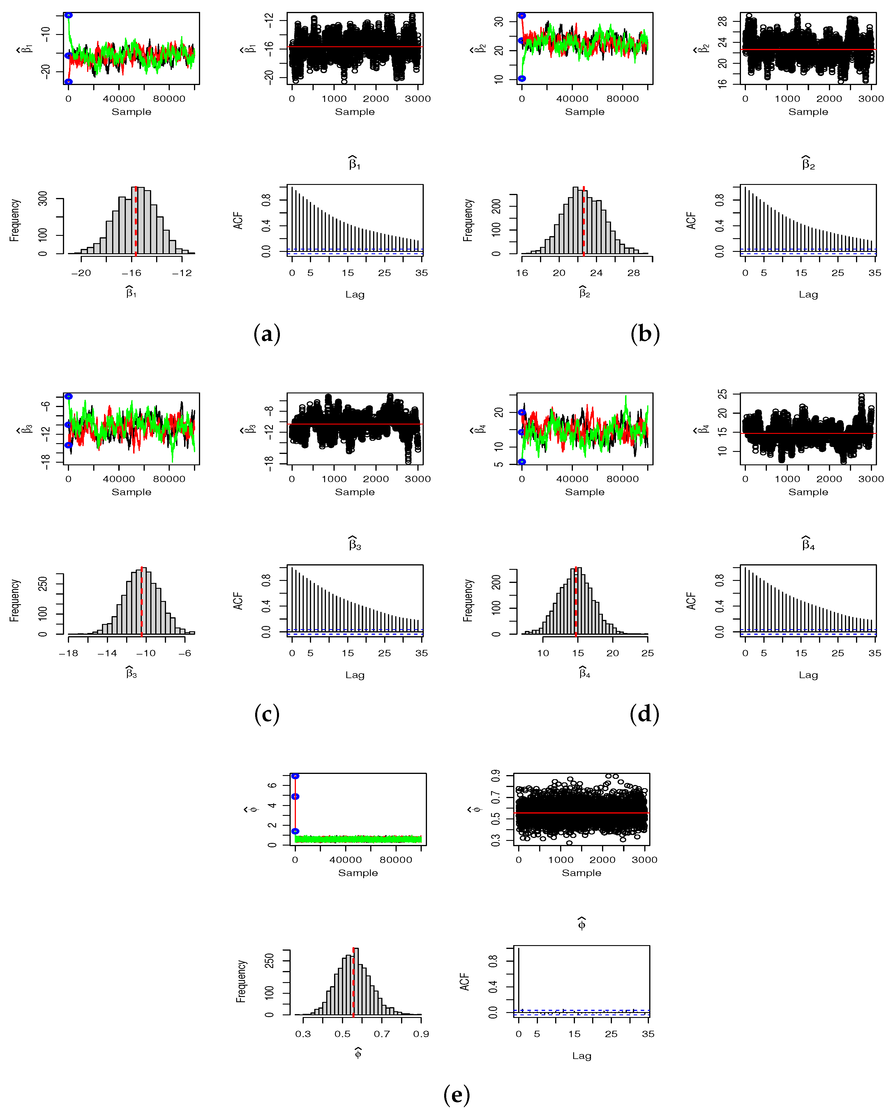
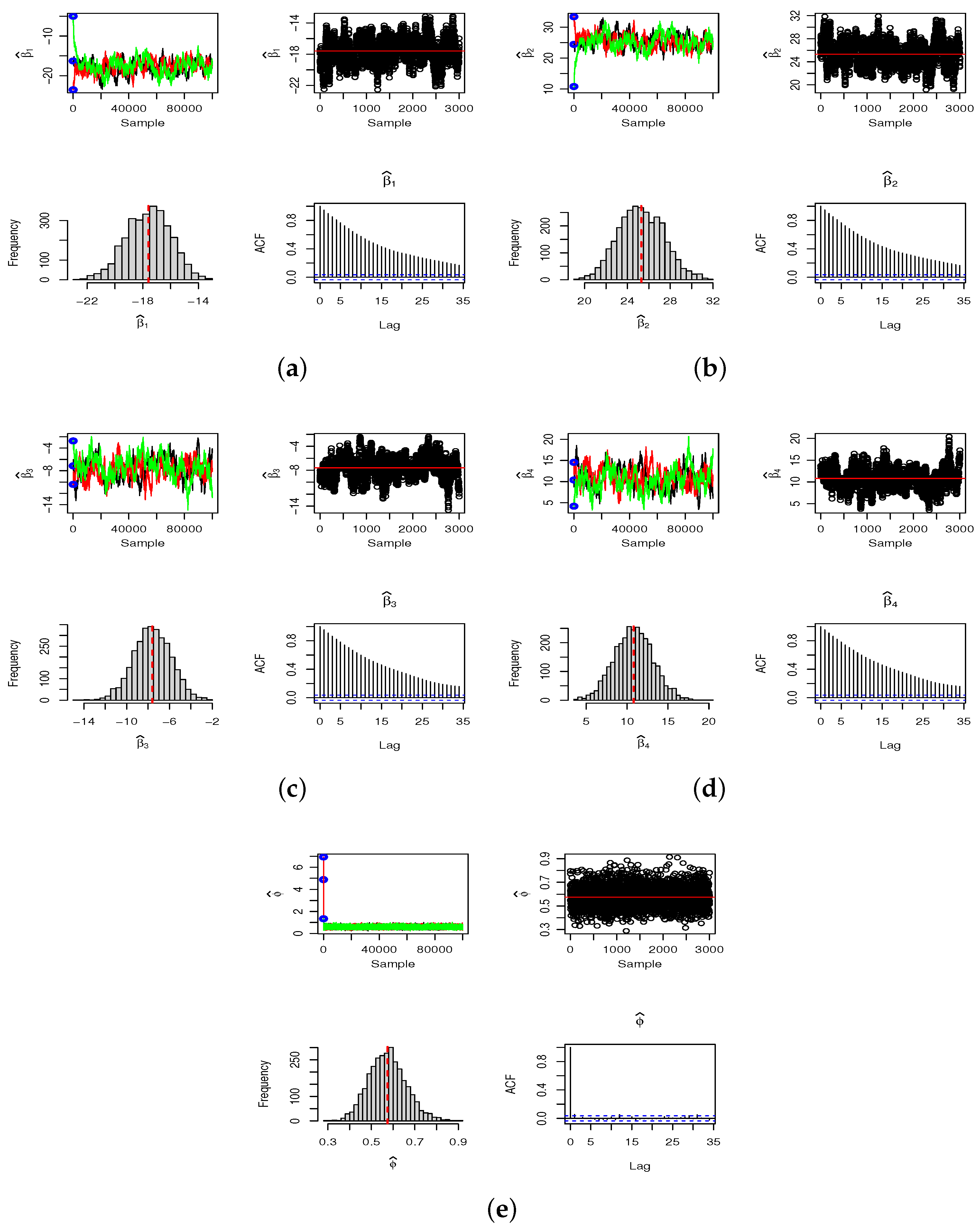
In this simulation study, we conducted a sensitivity analysis to evaluate the effect of initial conditions on the convergence of the generated chains. We tested three different chains, each initialized with conditions based on the mean of the prior, (i) 1.4 times the mean (i.e., plus 40%), and (ii) 0.4 times the mean (i.e., minus 60%). After verifying the burn-in period and ensuring the method’s convergence, we selected the mean of the prior distribution as the reference point for subsequent analysis.

We employed the SGHMC algorithm to generate 50,000 samples of $\mathit{\theta }$ from its full posterior distribution, discarding the first 50% as burn-in. This resulted in a chain consisting of 25,000 samples of $\mathit{\theta }$. The final sample was used to calculate the Monte Carlo estimates of each model parameter’s posterior mean and variance, as given by (19) and (20). We repeated this procedure $M=100$ times. With M estimates of the model parameters, we evaluated their performance using metrics such as mean bias (B), the ratio of mean squared error (MSE) to variance (Var), and the average Bayesian efficiency (BE), calculated for each model parameter ${\theta }_j$:

$$\begin{array}{ccc}\hfill B\left({\widehat{\theta }}_j\right)& =& {\displaystyle \frac{1}{M}}\sum _{k=1}^M\left({\widehat{\theta }}_j^{\left(k\right)}-{\theta }_j\right),\hfill \end{array}$$

(28)

$$\begin{array}{ccc}\hfill MSE\left({\widehat{\theta }}_j\right)& =& {\displaystyle \frac{1}{M}}\sum _{k=1}^M{({\widehat{\theta }}_j^{\left(k\right)}-{\theta }_j)}^2,\hfill \end{array}$$

(29)

$$\begin{array}{ccc}\hfill BE\left({\widehat{\theta }}_j\right)& =& {\displaystyle \frac{1}{M}}\sum _{k=1}^M{\displaystyle \frac{{\mathcal{V}}_{jj}^{\left(k\right)}}{{\widehat{\sigma }}_{{\theta }_j}^{2\left(k\right)}}},\hfill \end{array}$$

(30)

where ${\mathcal{V}}_{jj}^{\left(k\right)}$ is given by (25) and ${\widehat{\sigma }}_{{\theta }_j}^{2\left(k\right)}$ is given by (20) for each ${\widehat{\mathit{\theta }}}^{\left(k\right)}$, $k=1,\dots ,L$. Additionally, we have also computed the coverage probability ($CP$) of the Bayesian credible intervals expressed as percentages as

$$CP\left({\theta }_j\right)={\displaystyle \frac{100}{M}}\sum _{k=1}^M{\delta }_{\theta }^{\left(k\right)},$$

(31)

where ${\delta }_{\theta }^{\left(k\right)}$ assumes 1 if the kth Bayesian credible interval (BCI) contains the true value ${\theta }_j$ and 0 otherwise.

A summary of the $M=100$ simulations is shown in

Table 2. Simulation study. Estimation for the ZMPS($\mu ,\varphi ,p$) distribution using sample size $N=100$.

ZMPS	Parameters	$\mathit{N}(0,1)$			$\mathit{N}(0,100)$
	$\mathit{\theta }$	$\widehat{\mathit{\theta }}$	$\mathit{s}.\mathit{d}.$	HPD (95%)	$\widehat{\mathit{\theta }}$	$\mathit{s}.\mathit{d}.$	HPD (95%)
ZMP	${\beta }_{\mu ,1}=$−1.0	−1.061	0.306	(−1.573, −0.427)	−1.111	0.426	(−1.863, −0.299)
	${\beta }_{\mu ,2}=$  3.0	3.078	0.371	(2.341,  3.678)	3.135	0.511	(2.185,  4.025)
	${\beta }_{\omega ,1}=$−1.0	−1.025	0.312	(−1.604, −0.424)	−1.076	0.465	(−1.883, −0.212)
	${\beta }_{\omega ,2}=$  2.5	2.582	0.446	(1.915,  3.393)	2.686	0.768	(1.654,  4.262)
ZMNB	${\beta }_{\mu ,1}=$−1.0	−1.024	0.298	(−1.560, −0.380)	−1.102	0.559	(−2.261, −0.129)
	${\beta }_{\mu ,2}=$  3.0	3.035	0.403	(2.236, 3.811)	3.127	0.729	(1.668, 4.549)
	${\beta }_{\omega ,1}=$−1.5	−1.485	0.296	(−2.095, −0.883)	−1.507	0.476	(−2.443, −0.552)
	${\beta }_{\omega ,2}=$  2.0	1.967	0.459	(1.146, 2.889)	1.993	0.788	(0.661, 3.666)
	$\varphi =$  3.0	2.954	0.266	(2.423, 3.388)	2.939	0.265	(2.423, 3.398)
ZMGP	${\beta }_{\mu ,1}=$−1.0	−1.022	0.300	(−1.571, −0.412)	−1.124	0.605	(−2.377, −0.057)
	${\beta }_{\mu ,2}=$  3.0	3.053	0.419	(2.212,  3.829)	3.186	0.816	(1.519,  4.757)
	${\beta }_{\omega ,1}=$−1.5	−1.485	0.296	(−2.095, −0.883)	−1.507	0.476	(−2.443, −0.551)
	${\beta }_{\omega ,2}=$  2.0	1.967	0.459	(1.146,  2.889)	1.993	0.788	(0.661,  3.666)
	$\varphi =$  0.2	0.206	0.027	(0.153,  0.256)	0.208	0.027	(0.156,  0.256)
ZMCOMP	${\beta }_{\mu ,1}=$−3.5	−3.500	0.011	(−3.523, −3.478)	−3.523	0.098	(−3.716, −3.334)
	${\beta }_{\mu ,2}=$  2.0	1.999	0.012	(1.976,  2.022)	1.986	0.099	(1.785,  2.173)
	${\beta }_{\omega ,1}=$−1.0	−0.999	0.011	(−1.022, −0.976)	−0.998	0.090	(−1.103, −0.747)
	${\beta }_{\omega ,2}=$  0.5	0.500	0.011	(0.478,  0.523)	0.499	0.096	(0.345,  0.726)
	$\varphi =$  0.2	0.198	0.027	(0.125,  0.230)	0.196	0.027	(0.124,  0.231)

. In this summary, we can see the effect of the prior information on the calculation of the standard deviation (s.d.) and the amplitude of the highest posterior density (HPD) credibility interval for each parameter.

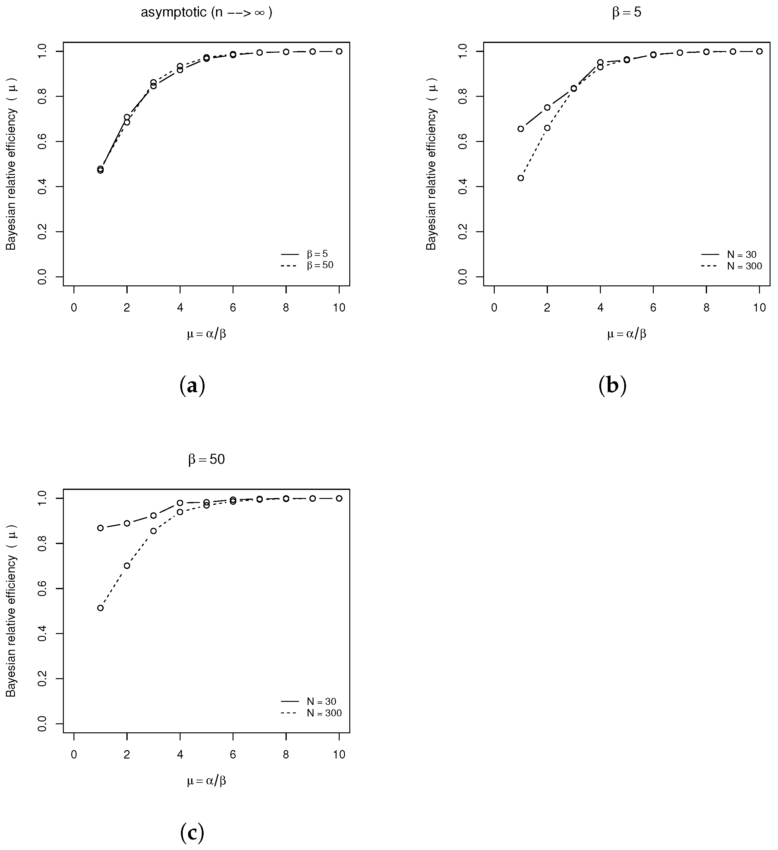
As previously discussed, the performance of the estimators using the metrics in (28)–(31) is presented in

Table 3. Simulation study. Results of the Bayesian efficiency for the ZMPS($\mu ,\varphi ,p$) distribution.

ZMPS	$\mathit{\theta }$	$\mathit{N}(0,1)$					$\mathit{N}(0,100)$
		B	MSE	$\mathit{PC}(\mathbf{\%})$	${\displaystyle \frac{\mathit{MSE}}{\mathit{Var}}}$	BE	B	MSE	$\mathit{CP}(\mathbf{\%})$	${\displaystyle \frac{\mathit{MSE}}{\mathit{Var}}}$	$\mathit{BE}$
ZMP	${\beta }_{\mu ,1}$	−0.061	0.097	97	1.039	1.00	−0.111	0.193	91	1.068	1.00
	${\beta }_{\mu ,2}$	0.078	0.144	99	1.044	1.00	0.135	0.279	89	1.069	1.00
	${\beta }_{\omega ,1}$	−0.025	0.098	98	1.006	1.00	−0.076	0.221	94	1.027	1.00
	${\beta }_{\omega ,2}$	0.082	0.205	99	1.033	1.00	0.186	0.625	94	1.059	1.00
ZMNB	${\beta }_{\mu ,1}$	−0.024	0.089	99	1.006	1.00	−0.102	0.323	94	1.033	1.00
	${\beta }_{\mu ,2}$	0.035	0.164	98	1.008	1.00	0.127	0.548	94	1.030	1.00
	${\beta }_{\omega ,1}$	0.014	0.088	97	1.002	1.00	−0.007	0.226	93	1.005	1.00
	${\beta }_{\omega ,2}$	−0.033	0.212	98	1.005	1.00	−0.007	0.621	94	1.007	1.00
	$\varphi$	−0.046	0.073	99	1.029	1.00	−0.061	0.074	99	1.052	1.00
ZMGP	${\beta }_{\mu ,1}$	−0.022	0.091	99	1.005	1.00	−0.124	0.382	93	1.042	0.97
	${\beta }_{\mu ,2}$	0.053	0.178	98	1.016	1.00	0.186	0.700	93	1.052	0.94
	${\beta }_{\omega ,1}$	0.014	0.088	97	1.002	1.00	−0.007	0.226	93	1.000	1.00
	${\beta }_{\omega ,2}$	−0.033	0.212	98	1.005	1.00	−0.007	0.621	94	1.000	1.00
	$\varphi$	0.006	0.001	99	1.052	0.83	0.008	0.001	99	1.083	0.82
ZMCP	${\beta }_{\mu ,1}$	0.002	0.001	99	1.004	1.00	0.023	0.010	99	1.056	0.76
	${\beta }_{\mu ,2}$	0.001	0.001	99	1.001	1.00	0.014	0.010	99	1.019	0.74
	${\beta }_{\omega ,1}$	0.003	0.001	99	1.000	0.93	0.002	0.008	99	1.000	0.74
	${\beta }_{\omega ,2}$	0.002	0.001	99	1.000	0.96	0.002	0.009	99	1.000	0.75
	$\varphi$	0.021	0.011	98	1.039	0.41	0.003	0.015	98	1.094	0.42

. The results show improved efficiency of the estimators when the prior distribution is more informative.

3.2. Application: Number of Femicide Cases

Violence against women encompasses a wide range of physical, psychological, sexual, and property-related attacks, often occurring on a continuum that can tragically culminate in murder, the most extreme manifestation of violence inflicted upon women.

Femicide refers to the murder of a woman specifically because she is a woman, typically driven by hatred, contempt, or a sense of lost control or ownership over women. Brazil’s Feminicide Law (Law 13.104 of 9 March 2015) classifies homicide as femicide when committed against a woman due to her gender. The law defines such crimes as those involving domestic or family violence, contempt, or discrimination against women and also includes femicide in the category of heinous crimes.

Of the five measures to combat gender-based violence recommended by the United Nations, Brazil has implemented only one: online services. This includes the “Red Light” campaign launched by the National Council of Justice and the Brazilian Association of Magistrates, which functions similarly to emergency alert systems. However, there has yet to be an assessment of the campaign’s impact on protecting women in violent situations. Factors contributing to the increase in gender-based violence include victims’ difficulty in reporting, a reduction in crime reporting at police stations, and a decline in the number of emergency protective measures granted to women.

This study aims to determine whether femicides increased during the COVID-19 pandemic. We analyze data from 642 municipalities in São Paulo for the years 2019 and 2020 [46], fitting ZMPS regression models with the Municipal Human Development Index (MHDI) as an explanatory variable. The MHDI, a key measure of municipal development in Brazil, evaluates three dimensions of human development: longevity, education, and income. It ranges from 0 to 1, with higher values indicating greater development. By interpreting the mean ${\mu }_i^{ZMPS}$ of the model and the parameter $p_i$ (which accounts for zero inflation or deflation) as functions of the MHDI, we gain insights into femicide patterns. A summary of the sample is presented in

Table 4. Frequency distribution and descriptive statistics of each sample referring to the number of femicides in 2019 and 2020 in 642 São Paulo municipalities.

Year	Frequency
	$y_i$	0	1	2	3	4	5	6	7	8	9	10	11	12	13	14	15
2019	$f_i$	254	132	56	45	27	23	16	13	7	7	3	1	5	2	2	4
2020	$f_i$	262	121	67	40	36	17	11	10	8	6	4	3	2	3	5	-
	$y_i$	16	17	18	19	20	21	22	23	24	25	26	27	28	29	30	>30
2019	$f_i$	2	3	2	3	3	2	3	2	-	2	3	1	2	1	1	15
2020	$f_i$	1	2	3	4	2	1	2	3	2	1	1	1	3	1	3	17

.

We apply the proposed Bayesian approach to fit ZMPS models to the femicide data, using the MHDI as a regressor. Specifically, we consider the zero-modified Poisson (ZMP), zero-modified negative binomial (ZMNB), zero-modified generalized Poisson (ZMGP), and zero-modified COM-Poisson (ZMCOMP) distributions. For the parameters $\mathit{\beta }\mu$ and $\mathit{\beta }w$, we use normal priors $N(0,{10}^2)$, while for $\varphi$, we apply a gamma prior $G(a_{\varphi },b_{\varphi })$ with $a_{\varphi }/b_{\varphi }=5$ and $a_{\varphi }/b_{\varphi }^2={10}^2$. We employ three information criteria, LogCPO (A8), EBIC (A9), and WAIC (A10), to identify the distribution that best fits the data, with higher LogCPO values and lower WAIC and EBIC values indicating better model performance. The values of these criteria for each fitted model are presented in

Table 5. Criteria for selecting the models that were fitted to the data on the number of femicide cases in 2019 and 2020.

Year	2019				2020
Criteria	ZMP	ZMNB	ZMGP	ZMCOMP	ZMP	ZMNB	ZMGP	ZMCOMP
LogCPO	2296	1376	1372	1481	2392	1372	1368	1492
WAIC	4658	2758	2767	2972	4866	2750	2750	3032
EBIC	4648	2783	2791	3000	4847	2775	2783	3044

, with the selected model for each sample highlighted in bold.

The three criteria identify the ZMNB model as the best fit for both 2019 and 2020. Posterior summaries and credible intervals for the parameters ${\mu }_i$, $\varphi$, and $p_i$ are presented in

Table 6. Posterior summaries and credible intervals of the parameters of ZMNB fitted to the number of femicide cases in 2019 and 2020.

Year	2019				2020
Parameter	Mean	Median	s.d.	CI (95%)	Mean	Median	s.d.	CI (95%)
${\beta }_{\mu ,0}$	−15.665	−15.594	1.579	(−18.883, −12.757)	−17.597	−17.528	1.592	(−20.839, −14.647)
${\beta }_{\mu ,1}$	22.629	22.558	2.098	(18.497, 26.587)	25.293	25.226	2.117	(21.200, 29.377)
${\beta }_{\omega ,0}$	−10.441	−10.443	1.808	(−14.178, −7.086)	−7.602	−7.613	1.751	(−11.150, −4.259)
${\mathit{\beta }}_{\omega ,1}$	14.724	14.692	2.454	(10.032, 19.653)	10.798	10.798	2.375	(6.339, 15.658)
$\varphi$	0.556	0.554	0.085	(0.396, 0.729)	0.574	0.572	0.086	(0.403, 0.741)

. The results are derived using three Markov chains, each containing 100,000 samples, initialized with distinct starting conditions. To minimize the effect of the burn-in period, we discard 25% of each chain and select every 75th value from the remaining 75% (thinning), which helps reduce autocorrelation within the chains. We use the resulting final sample of 3000 observations to compute the Bayesian Monte Carlo estimates. The convergence details of the SGHMC algorithm are provided in Appendix B. Figure 1 displays the estimated mean ${\mu }_i^{\left(ZMPS\right)}$ and the parameter $p_i$ for the ZMNB models based on data from 2019 and 2020.

In Figure 1a, we examine the mean number of reported femicides in relation to the MHDI. The graphs demonstrate that the mean number of notifications increases with the MHDI and is slightly higher during the COVID-19 pandemic. This trend indicates that municipalities with higher levels of development tend to report a greater mean number of femicides. This pattern is anticipated as more developed municipalities are likely to offer better protective measures for women and more effective crime reporting systems. The increase in reported cases in 2020, compared with the averages in 2019, can be attributed to the impacts of the pandemic.

The $p_i$ parameters are depicted as a function of the MHDI in Figure 1b. These parameters help interpret the frequency of zero observations within the sample. Typically, municipalities with lower mean notification numbers, ${\mu }_i$, are expected to exhibit zero inflation, meaning $p_i\le 1$. However, Figure 1b shows that for municipalities with an MHDI below 0.7 (i.e., those with low average ${\mu }_i$), the estimates of $p_i$ exceed 1. This indicates a deflation of zero observations at this level of the covariate, suggesting that municipalities with a low MHDI experience less zero inflation than expected. In fact, they report more cases than the standard model would predict ($p_i=1$). Furthermore, the increase in registrations during 2020, marked by a rise in deflation from zero, can be attributed to the impact of the COVID-19 pandemic, as seen in the comparison of $p_i$ estimates between 2019 and 2020.

4. Conclusions

The ZMPS distribution is constructed by modifying the zero probability of standard PS distributions. This flexible model accommodates count data with varying characteristics related to the frequency of zeros, including zero inflation and deflation, as well as different types of dispersion, such as overdispersion, equidispersion, and underdispersion. This property is particularly significant for ZMPS regression models, where zero inflation or deflation can manifest at different levels of covariates. As a result, the ZMPS class can be applied to model count datasets without requiring prior knowledge of zero inflation or deflation. Importantly, the ZMPS distribution includes PS distributions as a specific case.

This paper presents a Bayesian approach using the SGHMC algorithm to fit a ZMPS regression model. We demonstrate that estimates of ${\mu }_i$ and $\varphi$ can be obtained by focusing exclusively on the positive observations in a dataset and assuming a ZTPS distribution for these data. Based on this approach, we can evaluate relative efficiency losses by considering a measure of Bayesian information across different levels of prior information.

The estimation of the parameter $p_i$ enables the characterization of zero inflation ($0<p_i<1$) or zero deflation ($1<p_i<{\displaystyle \frac{1}{1-{\pi }_{PS}(0;{\mu }_i,\varphi )}}$). This parameter plays a key role in analyzing and interpreting the data, as discussed in Section 3.2. The ability to estimate $p_i$ is a significant strength of the ZMPS regression models.

Finally, as a practical application of the proposed ZMPS model, we analyzed the number of femicides in 642 municipalities in São Paulo for the years 2019 and 2020. In this dataset, zero observations are particularly significant, as the counts represent the number of women murdered. We fitted ZMPS regression models to these counts, utilizing the Municipal Human Development Index (MHDI) as an explanatory variable and estimating the $p_i$ parameter. This allowed for a more comprehensive analysis of the zero observations.

A limitation of the proposed model is the significant computational time and effort required to assess the impact of different initial conditions for a given dataset and to determine the appropriate chain length to ensure convergence and efficiency of the Monte Carlo estimators for the model parameters. Furthermore, the computational cost of fitting multiple models and applying a model selection criterion to identify the best PS distribution must be considered. In this study, we have used three criteria, LogCPO, EBIC, and WAIC, for Bayesian model selection.

A formulation of ZMPS regression models for longitudinal datasets that consider spatial correlations represents a natural extension for future research on the models presented in this paper.

References

1. Jain, G.C.; Consul, P.C. A Generalized Negative Binomial Distribution. SIAM J. Appl. Math. 1971, 21, 501–513. [Google Scholar] [CrossRef]
2. Ng, T. A new class of modified binomial distributions with applications to certain toxicological experiments. Commun. Stat. Theory Methods 1989, 18, 3477–3492. [Google Scholar] [CrossRef]
3. Johnson, N.L.; Kemp, A.W.; Kotz, S. Univariate Discrete Distributions, 3rd ed.; John Wiley & Sons: Hoboken, NJ, USA, 2005. [Google Scholar]
4. Consul, P.C.; Famoye, F. Lagrangian Probability Distributions; Birkhäuser: Boston, MA, USA, 2006. [Google Scholar]
5. Frome, E.L. The analysis of rates using Poisson regression model. Biometrics 1983, 39, 665–674. [Google Scholar] [CrossRef]
6. Frome, E.L.; Checkoway, H. Use of Poisson regression models in estimating incidence rates and ratios. Am. J. Epidemiol. 1985, 121, 309–323. [Google Scholar] [CrossRef] [PubMed]
7. Conigliani, C.; Castro, J.I.; O’Hagan, A. Bayesian Assessment of Goodness of Fit against Nonparametric Alternatives. Can. J. Stat. 2000, 28, 327–342. [Google Scholar] [CrossRef]
8. Bayarri, M.J.; Berger, J.O.; Datta, G.S. Objective Bayes Testing of Poisson Versus Inflated Poisson Models. Inst. Math. Stat. 2008, 3, 105–121. [Google Scholar]
9. Hinde, J.; Demetrio, C.G.B. Overdispersion: Models and estimation. Comput. Stat. Data Anal. 1998, 27, 151–170. [Google Scholar] [CrossRef]
10. Gupta, R.C. Modified Power Series Distribution and Some of its Applications. Indian J. Stat. 1974, 36, 288–298. [Google Scholar]
11. Consul, P.C. New Class of Location-Parameter Discrete Probability Distributions and Their Characterizations. Commun. Stat. Theory Methods 1990, 19, 4653–4666. [Google Scholar] [CrossRef]
12. Cordeiro, G.M.; Andrade, M.G.; de Castro, M. Power Series Generalized Nonlinear Models. Comput. Stat. Data Anal. 2009, 53, 1155–1166. [Google Scholar] [CrossRef]
13. M’Kendrick, A.G. Applications of mathematics to medical problems. Proc. Edinb. Math. Soc. 1926, 44, 98–103. [Google Scholar]
14. David, F.N.; Johnson, N.I. The truncated Poisson. Biometrics 1952, 8, 275–285. [Google Scholar] [CrossRef]
15. Cohen, A.C. An extension of a truncated Poisson distribution. Biometrics 1960, 16, 447–450. [Google Scholar] [CrossRef]
16. Umbach, D. On inference for a mixture of a Poisson and a degenerate distribution. Commun. Stat. Theory Methods 1981, 10, 299–306. [Google Scholar] [CrossRef]
17. Ridout, M.; Demétrio, C.G.B.; Hinde, J. Models for count data with many zeros. In Proceedings of the XIXth International Biometrics Conference, Cape Town, South Africa, 13–16 December 1998; pp. 179–192. [Google Scholar]
18. Dietz, E.; Böhning, D. On Estimation of the Poisson Parameter in Zero-Modified Poisson Models. Comput. Stat. Data Anal. 2000, 34, 441–459. [Google Scholar] [CrossRef]
19. Beckett, S.; Jee, J.; Ncube, T.; Pompilus, S.; Washington, Q.; Singh, A.; Pal, N. Zero-inflated Poisson (ZIP) distribution: Parameter estimation and applications to model data from natural calamities. Involv. A J. Math. 2014, 7, 751–767. [Google Scholar] [CrossRef]
20. Conceição, K.S.; Louzada, F.; Andrade, M.G.; Helou, E. Zero-modified power series distribution and its hurdle distribution version. J. Stat. Comput. Simul. 2017, 87, 1842–1862. [Google Scholar] [CrossRef]
21. Gelfand, A.; Smith, A. Sampling-based approaches to calculating marginal densities. J. Am. Stat. Assoc. 1990, 85, 398–409. [Google Scholar] [CrossRef]
22. Neal, R.M. Chapter 5: MCMC Using Hamiltonian Dynamics. In Handbook of Markov Chain Monte Carlo; CRC Press: New York, NY, USA, 2011; pp. 113–162. [Google Scholar]
23. Roberts, G.O.; Rosenthal, J.S. Optimal Scaling of Discrete Approximations to Langevin Diffusions. J. R. Stat. Soc. Ser. B Stat. Methodol. 1998, 60, 255–268. [Google Scholar] [CrossRef]
24. Roberts, G.; Stramer, O. Langevin diffusions and Metropolis-Hastings algorithms. Methodol. Comput. Appl. Probab. 2003, 4, 337–358. [Google Scholar] [CrossRef]
25. Girolami, M.; Calderhead, B. Riemann manifold Langevin and Hamiltonian Monte Carlo methods. J. R. Stat. Soc. Ser. B Stat. Methodol. 2011, 73, 123–214. [Google Scholar] [CrossRef]
26. Hoffman, M.D.; Gelman, A. The No-U-Turn Sampler: Adaptively Setting Path Lengths in Hamiltonian Monte Carlo. J. Mach. Learn. Res. 2014, 15, 1593–1623. [Google Scholar]
27. Welling, M.; Teh, Y.W. Bayesian learning via stochastic gradient Langevin dynamics. In Proceedings of the 28th International Conference on Machine Learning (ICML-11), Bellevue, WA, USA, 28 June–2 July 2011; pp. 681–688. [Google Scholar]
28. Chen, T.; Fox, E.; Guestrin, C. Stochastic Gradient Hamiltonian Monte Carlo. In Proceedings of the 31st International Conference on Machine Learning, Bejing, China, 22–24 June 2014; Xing, E.P., Jebara, T., Eds.; ACM Digital Library: New York, NY, USA, 2014; pp. 1683–1691. [Google Scholar]
29. Ding, N.; Fang, Y.; Babbush, R.; Chen, C.; Skeel, R.D.; Neven, H. Bayesian sampling using stochastic gradient thermostats. Adv. Neural Inf. Process. Syst. 2014, 27, 1–9. [Google Scholar]
30. Baker, J.; Fearnhead, P.; Fox, E.B.; Nemeth, C. sgmcmc: An R package for stochastic gradient Markov chain Monte Carlo. J. Stat. Softw. 2019, 91, 1–27. [Google Scholar] [CrossRef]
31. Nemeth, C.; Fearnhead, P. Stochastic Gradient Markov Chain Monte Carlo. J. Am. Stat. Assoc. 2021, 116, 433–450. [Google Scholar] [CrossRef]
32. Abadi, M.; Agarwal, A.; Barham, P.; Brevdo, E.; Chen, Z.; Citro, C.; Corrado, G.S.; Davis, A.; Dean, J.; Devin, M.; et al. TensorFlow: Large-Scale Machine Learning on Heterogeneous Systems. arXiv 2016, arXiv:1603.04467. [Google Scholar]
33. Luo, R. Approximate Inference on Structured Distributions Using Stochastic Dynamics. Doctoral Thesis, UCL (University College London), London, UK, 2024. [Google Scholar]
34. Guikema, S.D.; Coffelt, J.P. A flexible count data regression model for risk analysis. Risk Anal. 2008, 28, 213–223. [Google Scholar] [CrossRef] [PubMed]
35. Mullahy, J. Specification and testing of some modified count data models. J. Econom. 1986, 33, 341–365. [Google Scholar] [CrossRef]
36. Feng, C.X. Acomparison of zero-inflated and hurdle models for modeling zero-inflated count data. J. Stat. Distrib. Appl. 2021, 8, 1–19. [Google Scholar] [CrossRef] [PubMed]
37. Huayanay, A.; Bazán, J.; Cancho, V.; Dey, D. Performance of asymmetric links and correction methods for imbalanced data in binary regression. J. Stat. Comput. Simul. 2019, 89, 1694–1714. [Google Scholar] [CrossRef]
38. Gelman, A.; Hwang, J.; Vehtari, A. Understanding predictive information criteria for Bayesian models. Stat. Comput. 2014, 24, 997–1016. [Google Scholar] [CrossRef]
39. Gelfand, A.; Dey, K. Bayesian model choice: Asymptotics and exacts calculations. J. R. Stat. Soc. 1994, 56, 501–514. [Google Scholar] [CrossRef]
40. Carlin, B.; Louis, T. Bayes and Empirical Bayes Methods for Data Analysis, 2nd ed.; Chapman & Hall/CRC Texts in Statistical Science; Taylor & Francis: London, UK, 2010. [Google Scholar]
41. Watanabe, S. A widely applicable Bayesian information criterion. J. Mach. Learn. Res. 2013, 14, 867–897. [Google Scholar]
42. Ferreira, P. Extending Fisher’s measure of information. Biometrika 1981, 68, 695–698. [Google Scholar] [CrossRef]
43. Schützenberger, M.P. A generalization of the Frechet-Cramer inequality to the case of Bayes estimation. Bull. Amer. Math. Soc. 1957, 63, 142. [Google Scholar]
44. Pereira, C.A.B.; Stern, J.M. Evidence and Credibility: Full Bayesian Significance Test for Precise Hypotheses. Entropy 1999, 1, 99–110. [Google Scholar] [CrossRef]
45. Bernardo, J.; Smith, A. Bayesian Theory; Wiley Series in Probability and Statistics; Wiley: Hoboken, NJ, USA, 2009. [Google Scholar]
46. Datasus. Ministério da Saúde. DATASUS. Tabnet. 2022. Available online: https://datasus.saude.gov.br/mortalidade-desde-1996-pela-cid-10 (accessed on 4 January 2020).
47. Geweke, J. Evaluating the accuracy of sampling-based approaches to calculating posterior moments. J. R. Stat. Soc. 1994, 56, 501–514. [Google Scholar]
48. Gelman, A.; Rubin, D. Inference from iterative simulation using multiple sequences. Stat. Sci. 1992, 7, 457–511. [Google Scholar] [CrossRef]
49. Plummer, M.; Best, N.; Cowles, K.; Vines, K. CODA: Convergence Diagnosis and Output Analysis for MCMC. R News 2006, 6, 7–11. [Google Scholar]
Figure 1. The mean μ Z M N B (a) and the parameters p (b) fitted according to the MHDI for the 642 municipalities of São Paulo in 2019 and 2020.
Mathematics 13 00060 g001