Quantitative Controllability Metric for Disturbance Rejection in Linear Unstable Systems

Abstract

This paper introduces a novel Gramian-based quantitative metric to evaluate the disturbance rejection capabilities of linear unstable systems. The proposed metric addresses key limitations of the previously introduced degree of disturbance rejection (DoDR) metrics, including their dependency on the final time and numerical problems arising from differential equation computations. Specifically, this study defines the steady-state solution of the DoDR metric, which avoids numerical issues by relying only on solving four algebraic equations, even when the Gramian matrices diverge. This study further strengthens its contributions by providing rigorous mathematical proofs supporting the proposed method, ensuring a strong theoretical foundation. The derived results demonstrate that the proposed metric represents the sum of the steady-state input energies required to reject the disturbances in the asymptotically stable and anti-stable subsystems. Numerical examples demonstrated that the proposed metric maintained the physical meaning of the original DoDR while offering practical computational advantages. This study represents a significant step toward the efficient and reliable assessment of disturbance rejection capabilities in unstable systems.

1. Introduction

Controllability is a fundamental property of control systems, and is typically considered an essential requirement for their proper operation. The controllability of a system can be assessed through conventional methods, such as checking the rank of the controllability matrix, verifying the positive definiteness of the controllability Gramian, or using the Popov–Belevitch–Hautus (PBH) test. Although these tests are commonly used to check the controllability, they have certain limitations due to several reasons. First, they are highly sensitive to parameter perturbations in certain conditions [1] and provide only binary information on whether a system is controllable or not, without providing any information on how controllable the system is.

In order to resolve these problems, various metrics and methods for assessing the degree of controllability (DoC) were proposed over the decades, which include the controllability norm [2], extended PBH test [3], modal controllability [4], and minimum two-norms of the initial condition that cannot be regulated with bounded inputs [5]. Although these approaches provide physically meaningful information for the DoC of control systems, Gramian-based DoC metrics are most commonly employed due to the availability of the closed-form solution. Müller and Weber [6] paid attention to the fact that the minimum control input energy used to regulate a system is related to the controllability Gramian. Thus, they defined DoC metrics as three representative scalar values related to the controllability Gramian. Due to their intuitive and quantitative representation of controllability with closed-form solutions, Gramian-based DoC metrics have been widely used, and the concepts have also been extended to descriptor systems [7,8], nonlinear systems [9,10], bilinear systems [11,12], and network systems [13,14].

One of the primary applications of the Gramian-base DoC is the optimal actuator placement, as demonstrated in numerous studies [15,16,17,18]. However, standard DoC metrics do not account for external disturbances, even though the ability to reject disturbances is often an important consideration in actuator allocation. While some studies proposed actuator allocation methods that aim to maximize the disturbance rejection capability [19,20], these methods are typically based on transfer functions defined in the frequency domain and may not be suitable for disturbances with arbitrary frequency bands. Unlike the frequency domain approach, Mirza and Van Niekerk [21] introduced a disturbance sensitivity Gramian in the time domain, which quantifies the effect of the disturbance on closed-loop systems. This approach enables optimal actuator placement by minimizing the size of the Gramian. However, since the Gramian is defined for closed-loop systems, it depends on the control gain and may not be a representative metric for a given system. In order to resolve this problem, Kang et al. [22] proposed a metric based on the minimum input energy to reject the external disturbances for open-loop systems. This metric, which is often referred to as the degree of disturbance rejection (DoDR) capability in some related studies [23,24], is expressed with two Gramian matrices: the controllability and disturbance sensitivity Gramians for open-loop systems. Since the DoDR is also a Gramian-based metric, it gains the advantages of the Gramian-based DoC metric. Xia et al. [25] defined a Gramian-based metric that takes into account both the DoC and DoDR, providing a comprehensive measure of the controllability and disturbance rejection capability, and applied it to wind turbine systems [26,27]. Furthermore, Jeong and Park [28] extended the concept of DoDR to be applicable to active noise control (ANC) systems, and they utilized the metric to determine the optimal placement of control speakers.

While Gramian-based metrics provide closed-form solutions, obtaining the Gramian matrices requires solving differential equations, and their values depend on the final time, which can be a limitation in some cases. Although these problems can be resolved by using steady-state solutions of the Gramian matrices, which can be obtained by computing algebraic equations, it is only available for asymptotically stable systems since the Gramian matrices blow up for unstable systems. Zhou et al. [29] derived the Gramian matrices for unstable systems, and Shaker and Tahavori [17] used these Gramian matrices to define the DoC for unstable systems. However, these studies addressed stable and anti-stable modes separately, each in their own time domain. Therefore, the input energies considered in these works did not represent the control energy required for both stable and anti-stable modes simultaneously. Lee and Park [30] defined a DoC metric for unstable systems by deriving the minimum input energy required to simultaneously control both the stable and anti-stable subsystems, thus resolving the problems encountered in previous studies. This study demonstrates that the input energy required to control an unstable system is equivalent to the sum of the different input energies required to control each subsystem separately in the steady-state, allowing for simple computation of the metric.

Although definite and practical DoC metrics for linear unstable systems were proposed, evaluating their ability to reject disturbances remains a challenge. In particular, unstable systems, such as aerial vehicles [31,32,33] and walking robots [34,35,36], are inherently more susceptible to external disturbances, making robust control strategies [37] essential. As the design of robust control for disturbance rejection is important, assessing the system’s disturbance rejection capability itself is also crucial. However, as previously discussed, the DoDR metrics studied so far [25,26,27] are based on two Gramian matrices that diverge due to unstable modes in the systems. This divergence may lead to numerical issues, not only because solving differential equations is required but also due to potential problems in computing the inverse of the diverging Gramian matrices. Although a recent study [38] proposed a DoDR metric for undamped systems whose poles lie on the imaginary axis, allowing for computation without numerical issues despite the presence of diverging Gramian matrices, no study has yet addressed the computation of the DoDR metric for unstable systems whose poles lie in the right half-plane (RHP). Therefore, similar to the DoC for unstable systems, a solution is needed that allows for the straightforward computation of DoDR while maintaining its advantages and avoiding numerical problems.

In this paper, an intuitive and useful metric to quantify the disturbance rejection capabilities of unstable systems is proposed by deriving the steady-state solution of the DoDR. This study demonstrates that the steady-state solution can be obtained by solving only four algebraic equations, eliminating numerical issues, as opposed to the original time-dependent solution that required solving differential equations. Furthermore, the proofs of the theorems necessary to derive these results are also included in this paper, providing a rigorous mathematical foundation for the proposed metric. Numerical examples demonstrate the usefulness of the proposed metric. The following are the key distinguishing features of the proposed metric compared with existing metrics for assessing disturbance rejection capabilities:

• Applicable to unstable systems.
• Computed by solving only algebraic equations, allowing for straightforward calculations without numerical issues.
• Independent of final time considerations.

The rest of this paper is organized as follows: Section 2 provides the overview of the DoDR metric proposed in the previous study, including its definition, closed-form solution, and steady-state solution for asymptotically stable systems. Section 3 presents the derivation of the proposed metric. Several properties of Gramian matrices for unstable systems are also proved in this section to derive the steady-state solution. In Section 4, the usefulness of the proposed metric is demonstrated with numerical examples based on unstable systems with inverted pendulums. Finally, Section 5 concludes this paper.

2. Preliminaries

This section provides an overview of the DoDR metric proposed by Kang et al. [22], which forms the basis of the proposed metric for linear unstable systems derived in this paper.

2.1. Definition and Closed-Form Solution

Let us consider a linear time-invariant (LTI) controllable system:

$$\dot{x}\left(t\right)=Ax\left(t\right)+Bu\left(t\right)+Dw\left(t\right).$$

(1)

where $x\left(t\right)\in {\mathbf{R}}^n$, $u\left(t\right)\in {\mathbf{R}}^r$, and $w\left(t\right)\in {\mathbf{R}}^p$ denote the state, control input, and disturbance vectors, respectively, and A, B, and D are constant matrices with suitable dimensions. The disturbance is assumed to be zero-mean Gaussian white noise (GWN) with the known correlation function represented as

$$R_w\left(\tau \right)=E\left[w\left(t\right)w^T(t+\tau )\right]=S_w\delta \left(\tau \right).$$

(2)

where $R_w\left(\tau \right)$ and $S_w$ denote the correlation and covariance matrices of the disturbance, respectively. Although this paper assumes that the disturbance magnitude represented by the covariance matrix $S_w$ is known, as is common in related studies [22,38], its range can typically be inferred from system specifications or conditions, even when it is unknown. If no prior information about the magnitude of the disturbances is available for a control system, the matrix $S_w$ can serve as a weighting matrix representing the relative significance of disturbances, thereby enabling the evaluation of the disturbance rejection performance.

Equations (1) and (2) can be considered as a general LTI system, even in the presence of disturbances with an arbitrary bandwidth. This is possible because a disturbance with a specific bandwidth can be mathematically represented as the output of a filter, expressed as a state-space equation. Therefore, augmenting this filter into the system allows for the representation of the system with GWN disturbances, as depicted in Equations (1) and (2), without compromising the generality.

Then, the controllability metric for disturbance rejection $\rho \left(t_f\right)$, where $t_f$ denotes the final time, is defined as

$$\rho \left(t_f\right)=\underset{u}{\min }E\left[{\int }_0^{t_f}{u}^T\left(t\right)u\left(t\right)dt\right].$$

(3)

subject to $x\left(0\right)=0$, $x\left(t_f\right)=0$, and the equation in (1). The initial and final conditions are set to zero in order to focus on the disturbance rejection capability. According to the definition in Equation (3), a smaller value of $\rho \left(t_f\right)$ indicates a lower input energy required to suppress the disturbances, thereby indicating a better disturbance rejection capability of the system. In the definition, the types of disturbance controllers or control strategies are not considered. If the controller were included in the definition, the resulting metric would depend on the controller’s performance, which would prevent a clear evaluation of the system’s inherent disturbance rejection capability. Moreover, even well-known disturbance rejection techniques, such as sliding mode controllers [39] or adaptive controllers [40], are unable to drive the state to exactly zero at an arbitrary final time in many practical cases. Therefore, it is appropriate not to include the controller in the definition of the metric.

The closed-form solution of Equation (3) is given by

$$\rho \left(t_f\right)=\mathrm{tr}\left\{W_c^{-1}\left(t_f\right)W_d\left(t_f\right)\right\}.$$

(4)

where $W_c\left(t\right)$ and $W_d\left(t\right)$ represent the controllability Gramian and disturbance sensitivity Gramian, respectively, defined as

$$\begin{array}{c}{W}_c\left(t\right)={\int }_0^t{e}^{A\tau }B{B}^T{e}^{A^T\tau }d\tau .\end{array}$$

(5)

$$\begin{array}{c}{W}_d\left(t\right)={\int }_0^t{e}^{A\tau }D{S}_w{D}^T{e}^{A^T\tau }d\tau .\end{array}$$

(6)

It is clear that the matrix $W_c\left(t\right)$ is positive definite since we assumed that the system is controllable. In this paper, the derived solution in Equation (4) is named as DoDR, as referred to in previous studies [23,24]. The two Gramian matrices required to calculate DoDR can be obtained by solving the following two differential equations:

$$\begin{array}{c}\dot{W_c}\left(t\right)=A{W}_c\left(t\right)+W_c\left(t\right)A^T+B{B}^T.\end{array}$$

(7)

$$\begin{array}{c}\dot{W_d}\left(t\right)=A{W}_d\left(t\right)+W_d\left(t\right)A^T+D{S}_w{D}^T.\end{array}$$

(8)

2.2. Steady-State Solution for Asymptotically Stable Systems

Although DoDR has a physically meaningful value to evaluate the system’s disturbance rejection capability, it is required to solve two differential equations to calculate the metric, which is computationally expensive. Moreover, the DoDR in Equation (4) depends on the final time $t_f$. Such unexpected time dependency makes it difficult to determine the representative values for the system. Therefore, a steady-state solution of the DoDR is usually used to overcome the problem of computation burden and time dependency, instead of the time-dependent expression in Equation (4).

The Gramian matrices defined in Equations (5) and (6) have steady-state solutions if the system is asymptotically stable, i.e., A is a Hurwitz matrix. The steady-state solutions can be obtained by solving the following Lyapunov equations:

$$\begin{array}{c}A{\overline{W}}_c+{\overline{W}}_c{A}^T+B{B}^T=0.\end{array}$$

(9)

$$\begin{array}{c}A{\overline{W}}_d+{\overline{W}}_d{A}^T+D{S}_w{D}^T=0.\end{array}$$

(10)

where ${\overline{W}}_c$ and ${\overline{W}}_d$ denote the steady-state values of $W_c\left(t\right)$ and $W_d\left(t\right)$, respectively. Thus, the DoDR in the steady-state, $\overline{\rho }$, is given by

$$\overline{\rho }=\mathrm{tr}\left\{{\overline{W}}_c^{-1}{\overline{W}}_d\right\}.$$

(11)

Since the computation of the DoDR in the steady-state can be achieved by solving the algebraic equations in Equations (9) and (10) instead of the differential equations in (7) and (8), the problem of the computation burden can be resolved. Moreover, the use of steady-state Gramian matrices eliminates the problem of time-dependency. However, it should be noted that the steady-state Gramian matrices exist only for asymptotically stable systems. In the presence of unstable modes, i.e., if some eigenvalues of A are located in the right half-plane (RHP), the Gramian matrices diverge as the final time increases. For this reason, the expression for the DoDR in the steady-state in Equation (11) is not available for unstable systems, where the Gramian matrices diverge. Therefore, a new expression for the DoDR in the steady-state is required to quantify the disturbance rejection capability for unstable systems.

3. Proposed Metric to Quantify Disturbance Rejection Capabilities of Unstable Systems

In order to quantify the disturbance rejection capabilities of unstable systems, the proposed metric is defined as the steady-state solution of the DoDR for unstable systems, which is derived in this section. This derivation is based on the properties of the Gramian matrices in unstable systems, which are also derived in this section.

3.1. Properties of Gramian Matrices in Unstable Systems

If we consider an unstable system whose system matrix, i.e., A in Equation (1), has both positive and negative eigenvalues, without loss of generality, the system can be realized with the following state-space form:

$$\left[\begin{array}{c}{\dot{x}}_s\left(t\right)\\ {\dot{x}}_a\left(t\right)\end{array}\right]=\left[\begin{array}{cc}{A}_s& 0\\ 0& A_a\end{array}\right]\left[\begin{array}{c}{x}_s\left(t\right)\\ x_a\left(t\right)\end{array}\right]+\left[\begin{array}{c}{B}_s\\ B_a\end{array}\right]u\left(t\right)+\left[\begin{array}{c}{D}_s\\ D_a\end{array}\right]w\left(t\right)$$

(12)

where $x_s$, $A_s$, $B_s$, and $D_s$ denote the state, system matrix, input matrix, and disturbance input matrix of the asymptotically stable subsystem, respectively. Similarly, $x_a$, $A_a$, $B_a$, and $D_a$ denote those of the anti-stable subsystem, whose poles are all in the RHP. The realization in Equation (12) can be achieved through the similarity transform of the diagonal or Jordan canonical form [41].

According to Equation (12), the controllability Gramian for the unstable systems can be represented as

$$W_c\left(t\right)=\left[\begin{array}{cc}{W}_{cs}\left(t\right)& W_{csa}\left(t\right)\\ W_{cas}\left(t\right)& W_{ca}\left(t\right)\end{array}\right]$$

(13)

where $W_{cs}\left(t\right)$, $W_{csa}\left(t\right)$, $W_{cas}\left(t\right)$, and $W_{ca}\left(t\right)$ are the solutions of the following differential equations:

$$\begin{array}{cc}\hfill & {\dot{W}}_{cs}\left(t\right)=A_s{W}_{cs}\left(t\right)+W_{cs}\left(t\right)A_s^T+B_s{B}_s^T\hfill \end{array}$$

(14)

$$\begin{array}{cc}\hfill & {\dot{W}}_{ca}\left(t\right)=A_a{W}_{ca}\left(t\right)+W_{ca}\left(t\right)A_a^T+B_a{B}_a^T\hfill \end{array}$$

(15)

$$\begin{array}{cc}\hfill & {\dot{W}}_{csa}\left(t\right)=A_s{W}_{csa}\left(t\right)+W_{csa}\left(t\right)A_a^T+B_s{B}_a^T\hfill \end{array}$$

(16)

$$\begin{array}{cc}\hfill & {\dot{W}}_{cas}\left(t\right)=A_a{W}_{cas}\left(t\right)+W_{cas}\left(t\right)A_s^T+B_a{B}_s^T\hfill \end{array}$$

(17)

Similarly, the disturbance sensitivity Gramian for an unstable system can be written as

$$W_d\left(t\right)=\left[\begin{array}{cc}{W}_{ds}\left(t\right)& W_{dsa}\left(t\right)\\ W_{das}\left(t\right)& W_{da}\left(t\right)\end{array}\right]$$

(18)

where $W_{ds}\left(t\right)$, $W_{dsa}\left(t\right)$, $W_{das}\left(t\right)$, and $W_{da}\left(t\right)$ are the solutions of the following differential equations:

$$\begin{array}{cc}\hfill & {\dot{W}}_{ds}\left(t\right)=A_s{W}_{ds}\left(t\right)+W_{ds}\left(t\right)A_s^T+D_s{S}_w{D}_s^T\hfill \end{array}$$

(19)

$$\begin{array}{cc}\hfill & {\dot{W}}_{da}\left(t\right)=A_a{W}_{da}\left(t\right)+W_{da}\left(t\right)A_a^T+D_a{S}_w{D}_a^T\hfill \end{array}$$

(20)

$$\begin{array}{cc}\hfill & {\dot{W}}_{dsa}\left(t\right)=A_s{W}_{dsa}\left(t\right)+W_{dsa}\left(t\right)A_a^T+D_s{S}_w{D}_a^T\hfill \end{array}$$

(21)

$$\begin{array}{cc}\hfill & {\dot{W}}_{das}\left(t\right)=A_a{W}_{das}\left(t\right)+W_{das}\left(t\right)A_s^T+D_a{S}_w{D}_s^T\hfill \end{array}$$

(22)

Since all eigenvalues of $A_s$ are in the LHP, the steady-state solution for Equations (14) and (19) can be obtained by solving the following algebraic Lyapunov equation:

$$\begin{array}{c}{A}_s{\overline{W}}_{cs}+{\overline{W}}_{cs}{A}_s^T+B_s{B}_s^T=0\end{array}$$

(23)

$$\begin{array}{c}{A}_s{\overline{W}}_{ds}+{\overline{W}}_{ds}{A}_s^T+D_s{S}_w{D}_s^T=0\end{array}$$

(24)

where ${\overline{W}}_{cs}$ and ${\overline{W}}_{ds}$ denote the steady-state values of $W_{cs}\left(t\right)$ and $W_{ds}\left(t\right)$, respectively.

In order to derive the steady-state solution of the DoDR for unstable systems, we define new Gramian matrices, $M_c\left(t\right)$ and $M_d\left(t\right)$, as shown in the following equations:

$$\begin{array}{c}{M}_c\left(t\right)={\int }_0^t{e}^{-A\tau }B{B}^T{e}^{-A^T\tau }d\tau \end{array}$$

(25)

$$\begin{array}{c}{M}_d\left(t\right)={\int }_0^t{e}^{-A\tau }D{S}_w{D}^T{e}^{-A^T\tau }d\tau \end{array}$$

(26)

The newly defined Gramian matrices in Equations (25) and (26) are obtained from the previously defined Gramian matrices in Equations (5) and (6) by replacing the system matrix A with $-A$. Similar to the expressions shown in Equations (13) to (22), $M_c\left(t\right)$ and $M_d\left(t\right)$ for unstable systems can also be represented as follows:

$$\begin{array}{c}{M}_c\left(t\right)=\left[\begin{array}{cc}{M}_{cs}\left(t\right)& M_{csa}\left(t\right)\\ M_{cas}\left(t\right)& M_{ca}\left(t\right)\end{array}\right]\end{array}$$

(27)

$$\begin{array}{c}{M}_d\left(t\right)=\left[\begin{array}{cc}{M}_{ds}\left(t\right)& M_{dsa}\left(t\right)\\ M_{das}\left(t\right)& M_{da}\left(t\right)\end{array}\right]\end{array}$$

(28)

where $M_{cs}\left(t\right)$, $M_{csa}\left(t\right)$, $M_{cas}\left(t\right)$, $M_{ca}\left(t\right)$, $M_{ds}\left(t\right)$, $M_{dsa}\left(t\right)$, $M_{das}\left(t\right)$, and $M_{da}\left(t\right)$ are the solutions of the following differential equations:

$$\begin{array}{cc}\hfill & {\dot{M}}_{cs}\left(t\right)=-A_s{M}_{cs}\left(t\right)-M_{cs}\left(t\right)A_s^T+B_s{B}_s^T\hfill \end{array}$$

(29)

$$\begin{array}{cc}\hfill & {\dot{M}}_{ca}\left(t\right)=-A_a{M}_{ca}\left(t\right)-M_{ca}\left(t\right)A_a^T+B_a{B}_a^T\hfill \end{array}$$

(30)

$$\begin{array}{cc}\hfill & {\dot{M}}_{csa}\left(t\right)=-A_s{M}_{csa}\left(t\right)-M_{csa}\left(t\right)A_a^T+B_s{B}_a^T\hfill \end{array}$$

(31)

$$\begin{array}{cc}\hfill & {\dot{M}}_{cas}\left(t\right)=-A_a{M}_{cas}\left(t\right)-M_{cas}\left(t\right)A_s^T+B_a{B}_s^T\hfill \end{array}$$

(32)

$$\begin{array}{cc}\hfill & {\dot{M}}_{ds}\left(t\right)=-A_s{M}_{ds}\left(t\right)-M_{ds}\left(t\right)A_s^T+D_s{S}_w{D}_s^T\hfill \end{array}$$

(33)

$$\begin{array}{cc}\hfill & {\dot{M}}_{da}\left(t\right)=-A_a{M}_{da}\left(t\right)-M_{da}\left(t\right)A_a^T+D_a{S}_w{D}_a^T\hfill \end{array}$$

(34)

$$\begin{array}{cc}\hfill & {\dot{M}}_{dsa}\left(t\right)=-A_s{M}_{dsa}\left(t\right)-M_{dsa}\left(t\right)A_a^T+D_s{S}_w{D}_a^T\hfill \end{array}$$

(35)

$$\begin{array}{cc}\hfill & {\dot{M}}_{das}\left(t\right)=-A_a{M}_{das}\left(t\right)-M_{das}\left(t\right)A_s^T+D_a{S}_w{D}_s^T\hfill \end{array}$$

(36)

Since all eigenvalues of $A_a$ are in the RHP, the eigenvalues of $-A_a$ are all in the LHP. Thus, the steady-state solution for Equations (30) and (34) can also be obtained by solving the following algebraic equation:

$$\begin{array}{c}{A}_a{\overline{M}}_{ca}+{\overline{M}}_{ca}{A}_a^T-B_a{B}_a^T=0\end{array}$$

(37)

$$\begin{array}{c}{A}_a{\overline{M}}_{da}+{\overline{M}}_{da}{A}_a^T-D_a{S}_w{D}_a^T=0\end{array}$$

(38)

The following relationship holds among the Gramian matrices defined so far.

Lemma 1.

The matrices $M_c\left(t\right)$ and $M_d\left(t\right)$ have the following relationships with the controllability and disturbance sensitivity Gramians:

$$\begin{array}{c}{M}_c\left(t\right)=e^{-At}{W}_c\left(t\right)e^{-A^{T}t}\end{array}$$

(39)

$$\begin{array}{c}{M}_d\left(t\right)=e^{-At}{W}_d\left(t\right)e^{-A^{T}t}\end{array}$$

(40)

Proof. 

From Equation (25), the following equations hold:

$$\begin{array}{cc}\hfill M_c\left(t\right)& ={\int }_0^t{e}^{-A\tau }B{B}^T{e}^{-A^T\tau }d\tau \hfill \\ \hfill & =e^{-At}\left\{{\int }_0^t{e}^{A(t-\tau )}B{B}^T{e}^{A^T(t-\tau )}d\tau \right\}{e}^{-A^{T}t}\hfill \\ \hfill & =e^{-At}{W}_c\left(t\right)e^{-A^{T}t}\hfill \end{array}$$

(41)

This completes the proof of Equation (39). The proof of Equation (40) can be achieved in a similar way and has been omitted for brevity. □

Corollary 1.

The matrices $M_{cs}\left(t\right)$, $M_{csa}\left(t\right)$, $M_{cas}\left(t\right)$, $M_{ca}\left(t\right)$, $M_{ds}\left(t\right)$, $M_{dsa}\left(t\right)$, $M_{das}\left(t\right)$, and $M_{da}\left(t\right)$ have the following relationships with the matrices $W_{cs}\left(t\right)$, $W_{csa}\left(t\right)$, $W_{cas}\left(t\right)$, $W_{ca}\left(t\right)$, $W_{ds}\left(t\right)$, $W_{dsa}\left(t\right)$, $W_{das}\left(t\right)$, and $W_{da}\left(t\right)$.

$$\begin{array}{cc}\hfill & M_{cs}\left(t\right)=e^{-A_{s}t}{W}_{cs}\left(t\right)e^{-A_s^{T}t}\hfill \end{array}$$

(42)

$$\begin{array}{cc}\hfill & M_{csa}\left(t\right)=e^{-A_{s}t}{W}_{csa}\left(t\right)e^{-A_a^{T}t}\hfill \end{array}$$

(43)

$$\begin{array}{cc}\hfill & M_{cas}\left(t\right)=e^{-A_{a}t}{W}_{cas}\left(t\right)e^{-A_s^{T}t}\hfill \end{array}$$

(44)

$$\begin{array}{cc}\hfill & M_{ca}\left(t\right)=e^{-A_{a}t}{W}_{ca}\left(t\right)e^{-A_a^{T}t}\hfill \end{array}$$

(45)

$$\begin{array}{cc}\hfill & M_{ds}\left(t\right)=e^{-A_{s}t}{W}_{ds}\left(t\right)e^{-A_s^{T}t}\hfill \end{array}$$

(46)

$$\begin{array}{cc}\hfill & M_{dsa}\left(t\right)=e^{-A_{s}t}{W}_{dsa}\left(t\right)e^{-A_a^{T}t}\hfill \end{array}$$

(47)

$$\begin{array}{cc}\hfill & M_{das}\left(t\right)=e^{-A_{a}t}{W}_{das}\left(t\right)e^{-A_s^{T}t}\hfill \end{array}$$

(48)

$$\begin{array}{cc}\hfill & M_{da}\left(t\right)=e^{-A_{a}t}{W}_{da}\left(t\right)e^{-A_a^{T}t}\hfill \end{array}$$

(49)

Proof. 

$e^{At}$ in Equations (39) and (40) can be rewritten as

$$e^{At}=\left[\begin{array}{cc}{e}^{A_{s}t}& 0\\ 0& e^{A_{a}t}\end{array}\right]$$

(50)

Substituting Equations (13), (27), and (50) into (39) yields

$$\begin{array}{cc}\hfill M_c\left(t\right)& =\left[\begin{array}{cc}{M}_{cs}\left(t\right)& M_{csa}\left(t\right)\\ M_{cas}\left(t\right)& M_{ca}\left(t\right)\end{array}\right]\hfill \\ \hfill & =e^{-At}\left[\begin{array}{cc}{W}_{cs}\left(t\right)& W_{csa}\left(t\right)\\ W_{cas}\left(t\right)& W_{ca}\left(t\right)\end{array}\right]e^{-A^{T}t}\hfill \\ \hfill & =\left[\begin{array}{cc}{e}^{-A_{s}t}{W}_{cs}\left(t\right)e^{-A_s^{T}t}& e^{-A_{s}t}{W}_{csa}\left(t\right)e^{-A_a^{T}t}\\ e^{-A_{a}t}{W}_{cas}\left(t\right)e^{-A_s^{T}t}& e^{-A_{a}t}{W}_{ca}\left(t\right)e^{-A_a^{T}t}\end{array}\right]\hfill \end{array}$$

(51)

This completes the proofs of Equations (42) to (45). The proofs of Equations (46) to (49) can be achieved in a similar way and have been omitted for brevity. □

As represented in Equation (4), we need to understand the properties of the inverse of the controllability Gramian in order to derive the steady-state solution of the DoDR for unstable systems. The inverse of the Gramian can be represented as the following blockwise inversion:

$$W_c^{-1}\left(t\right)=\left[\begin{array}{cc}{W}_{cs}^{-1}\left(t\right)+V_1\left(t\right)& -V_2\left(t\right)\\ -V_3\left(t\right)& V_4\left(t\right)\end{array}\right]$$

(52)

where

$$\begin{array}{cc}\hfill V_1\left(t\right)& =W_{cs}^{-1}\left(t\right)W_{csa}\left(t\right)V_4\left(t\right)W_{cas}\left(t\right)W_{cs}^{-1}\left(t\right)\hfill \end{array}$$

(53)

$$\begin{array}{cc}\hfill V_2\left(t\right)& =V_3^T\left(t\right)=W_{cs}^{-1}\left(t\right)W_{csa}\left(t\right)V_4\left(t\right)\hfill \end{array}$$

(54)

$$\begin{array}{cc}\hfill V_4\left(t\right)& ={\left\{W_{ca}\left(t\right)-W_{cas}\left(t\right)W_{cs}^{-1}\left(t\right)W_{csa}\left(t\right)\right\}}^{-1}\hfill \end{array}$$

(55)

The matrices $V_1\left(t\right)$, $V_2\left(t\right)$, $V_3\left(t\right)$, and $V_4\left(t\right)$ defined in Equations (53) to (55), and the inverse of the controllability Gramian, $W_c^{-1}\left(t\right)$, have the following properties.

Lemma 2.

The matrices $V_1\left(t\right)$, $V_2\left(t\right)$, $V_3\left(t\right)$, and $V_4\left(t\right)$ converge to zero matrices with appropriate dimensions as the time goes to infinity, i.e.,

$$\begin{array}{cc}\hfill \underset{t\to \infty }{lim}{V}_1\left(t\right)& =0\hfill \end{array}$$

(56)

$$\begin{array}{cc}\hfill \underset{t\to \infty }{lim}{V}_2\left(t\right)& =\underset{t\to \infty }{lim}{V}_3^T\left(t\right)=0\hfill \end{array}$$

(57)

$$\begin{array}{cc}\hfill \underset{t\to \infty }{lim}{V}_4\left(t\right)& =0\hfill \end{array}$$

(58)

Proof. 

The matrix $V_4\left(t\right)$ can be rewritten as the following equation by using the equations in (43) to (45):

$$V_4\left(t\right)=e^{-A_a^{T}t}{\left\{M_{ca}\left(t\right)-K_{cas}\left(t\right)W_{cs}^{-1}\left(t\right)K_{csa}\left(t\right)\right\}}^{-1}{e}^{-A_{a}t}$$

(59)

where

$$K_{csa}\left(t\right)=K_{cas}^T\left(t\right)=W_{csa}\left(t\right)e^{-A_a^{T}t}$$

(60)

The time derivative of $K_{csa}\left(t\right)$ is given by

$${\dot{K}}_{csa}\left(t\right)=A_s{K}_{csa}\left(t\right)+B_s{B}_a^T{e}^{-A_a^{T}t}$$

(61)

Since $A_s$ is negative definite, and $B_a^T{e}^{-A_a^{T}t}$ converges to a zero matrix as time goes to infinity due to the positive definiteness of $A_a$, the columns of $K_{csa}\left(t\right)$ can be regarded as the state vectors for the asymptotically stable system with the inputs converging to zero. Thus, it is clear that

$$\underset{t\to \infty }{lim}{K}_{csa}\left(t\right)=\underset{t\to \infty }{lim}{K}_{cas}^T\left(t\right)=0$$

(62)

Since $W_{cs}\left(t\right)$ and $M_{ca}\left(t\right)$ in Equation (59) are positive definite and have finite steady-state solutions, as represented in Equations (23) and (37), Equation (58) can be proved by substituting Equation (62) into the time limit of Equation (59). In the same manner, the matrices $V_1\left(t\right)$, $V_2\left(t\right)$, and $V_3\left(t\right)$ can also be rewritten as the following equations:

$$\begin{array}{cc}\hfill & V_1\left(t\right)=W_{cs}^{-1}\left(t\right)K_{csa}\left(t\right){\left\{M_{ca}\left(t\right)-K_{cas}\left(t\right)W_{cs}^{-1}\left(t\right)K_{csa}\left(t\right)\right\}}^{-1}{K}_{cas}\left(t\right)W_{cs}^{-1}\left(t\right)\hfill \end{array}$$

(63)

$$\begin{array}{cc}\hfill & V_2\left(t\right)=W_{cs}^{-1}\left(t\right)K_{csa}\left(t\right){\left\{M_{ca}\left(t\right)-K_{cas}\left(t\right)W_{cs}^{-1}\left(t\right)K_{csa}\left(t\right)\right\}}^{-1}{e}^{-A_{a}t}\hfill \end{array}$$

(64)

$$\begin{array}{cc}\hfill & V_3\left(t\right)=e^{-A_a^{T}t}{\left\{M_{ca}\left(t\right)-K_{cas}\left(t\right)W_{cs}^{-1}\left(t\right)K_{csa}\left(t\right)\right\}}^{-1}{K}_{cas}\left(t\right)W_{cs}^{-1}\left(t\right)\hfill \end{array}$$

(65)

Therefore, Equations (56) and (57) can be proved in the same way as Equation (58). This completes the proof. □

Corollary 2.

The inverse of the controllability Gramian for unstable systems has a steady-state solution as the following:

$${\overline{W}}_c^{-1}=\underset{t\to \infty }{lim}{W}_c^{-1}\left(t\right)=\left[\begin{array}{cc}{\overline{W}}_{cs}^{-1}& 0\\ 0& 0\end{array}\right]$$

(66)

Proof. 

It follows directly from Lemma 2. □

As shown in Equation (66), only the stable subsystem affects the inverse of the controllability Gramian in the steady-state. This means that the anti-stable subsystem does not contribute to the inverse of the Gramian in the steady-state. Meanwhile, the block matrices $W_{dsa}\left(t\right)$, $W_{das}\left(t\right)$, and $W_{da}\left(t\right)$ in Equation (18) contain unstable modes and diverge to infinity over time, while $V_1\left(t\right)$, $V_2\left(t\right)$, $V_3\left(t\right)$, and $V_4\left(t\right)$ converge to zero. Therefore, although the anti-stable subsystem does not contribute to the inverse of the controllability Gramian in the steady-state, it cannot be considered to have no effect on the DoDR in the steady-state.

3.2. Steady-State Solution for Unstable Systems

Using the previously described properties of the Gramian matrices, the steady-state solution of the DoDR for unstable systems is derived as follows. First, it is worth noting the following properties of the DoDR for anti-stable systems.

Theorem 1.

If a given system is anti-stable, i.e., the matrix A in Equation (1) is positive definite, then the steady-state solution of the DoDR for the system is given by

$$\overline{\rho }=\mathrm{tr}\left({\overline{M}}_c^{-1}{\overline{M}}_d\right)$$

(67)

where ${\overline{M}}_c$ and ${\overline{M}}_d$ are the steady-state solutions for $M_c\left(t\right)$ and $M_d\left(t\right)$, respectively, which can be obtained from the following algebraic equations:

$$\begin{array}{c}A{\overline{M}}_c+{\overline{M}}_c{A}^T-B{B}^T=0\end{array}$$

(68)

$$\begin{array}{c}A{\overline{M}}_d+{\overline{M}}_d{A}^T-D{S}_w{D}^T=0\end{array}$$

(69)

Proof. 

The time-dependent solution of the DoDR in Equation (4) can be rewritten as

$$\begin{array}{cc}\hfill \rho \left(t_f\right)& =\mathrm{tr}\left\{W_c^{-1}\left(t_f\right)W_d\left(t_f\right)\right\}\hfill \\ \hfill & =\mathrm{tr}\left\{W_c^{-1}\left(t_f\right)e^{A{t}_f}{e}^{-A{t}_f}{W}_d\left(t_f\right)e^{-A^T{t}_f}{e}^{A^T{t}_f}\right\}\hfill \end{array}$$

(70)

From the property of the trace function, Equation (70) can be rewritten as

$$\begin{array}{cc}\hfill & \rho \left(t_f\right)=\mathrm{tr}\left\{e^{A^T{t}_f}{W}_c^{-1}\left(t_f\right)e^{A{t}_f}{e}^{-A{t}_f}{W}_d\left(t_f\right)e^{-A^T{t}_f}\right\}\hfill \\ \hfill & =\mathrm{tr}\left[{\left\{e^{-A{t}_f}{W}_c\left(t_f\right)e^{-A^T{t}_f}\right\}}^{-1}\left\{e^{-A{t}_f}{W}_d\left(t_f\right)e^{-A^T{t}_f}\right\}\right]\hfill \end{array}$$

(71)

Substituting Equations (39) and (40) into equation (71) yields

$$\rho \left(t_f\right)=\mathrm{tr}\left\{M_c^{-1}\left(t_f\right)M_d\left(t_f\right)\right\}$$

(72)

Since the matrix A is positive definite, i.e., $-A$ is a Hurwitz matrix, the matrices $M_c\left(t\right)$ and $M_d\left(t\right)$ in Equation (72) have the steady-state solutions that can be obtained from Equations (68) and (69). This completes the proof. □

The aforementioned property shows that the steady-state value of the DoDR for anti-stable systems can also be obtained by solving algebraic equations, similarly to stable systems. Based on this, the DoDR for unstable systems is derived as the following.

Theorem 2.

The steady-state solution of DoDR for unstable systems is given by

$$\overline{\rho }=\mathrm{tr}\left({\overline{W}}_{cs}^{-1}{\overline{W}}_{ds}\right)+\mathrm{tr}\left({\overline{M}}_{ca}^{-1}{\overline{M}}_{da}\right)$$

(73)

Proof. 

Substituting Equations (18) and (52) into Equation (4) yields

$$\rho \left(t_f\right)={\rho }_1\left(t_f\right)+{\rho }_2\left(t_f\right)-{\rho }_3\left(t_f\right)-{\rho }_4\left(t_f\right)+{\rho }_5\left(t_f\right)$$

(74)

where

$$\begin{array}{cc}\hfill {\rho }_1\left(t\right)& =\mathrm{tr}\left\{W_{cs}^{-1}\left(t\right)W_{ds}\left(t\right)\right\}\hfill \end{array}$$

(75)

$$\begin{array}{cc}\hfill {\rho }_2\left(t\right)& =\mathrm{tr}\left\{V_1\left(t\right)W_{ds}\left(t\right)\right\}\hfill \end{array}$$

(76)

$$\begin{array}{cc}\hfill {\rho }_3\left(t\right)& =\mathrm{tr}\left\{V_2\left(t\right)W_{das}\left(t\right)\right\}\hfill \end{array}$$

(77)

$$\begin{array}{cc}\hfill {\rho }_4\left(t\right)& =\mathrm{tr}\left\{V_3\left(t\right)W_{dsa}\left(t\right)\right\}\hfill \end{array}$$

(78)

$$\begin{array}{cc}\hfill {\rho }_5\left(t\right)& =\mathrm{tr}\left\{V_4\left(t\right)W_{da}\left(t\right)\right\}\hfill \end{array}$$

(79)

Since $W_{cs}\left(t\right)$ and $W_{ds}\left(t\right)$ have steady-state solutions, it is clear that

$$\begin{array}{cc}\hfill \underset{t\to \infty }{lim}{\rho }_1\left(t\right)& =\mathrm{tr}\left\{{\overline{W}}_{cs}^{-1}{\overline{W}}_{ds}\right\}\hfill \end{array}$$

(80)

$$\begin{array}{cc}\hfill \underset{t\to \infty }{lim}{\rho }_2\left(t\right)& =0\hfill \end{array}$$

(81)

Substituting Equation (64) into Equation (77) yields

$${\rho }_3\left(t\right)=\mathrm{tr}\left\{W_{cs}^{-1}{K}_{csa}{(M_{ca}-K_{cas}{W}_{cs}^{-1}{K}_{csa})}^{-1}{K}_{das}\right\}$$

(82)

where

$$K_{dsa}\left(t\right)=K_{das}^T\left(t\right)=W_{dsa}\left(t\right)e^{-A_a^{T}t}$$

(83)

Similar to $K_{csa}\left(t\right)$ and $K_{cas}\left(t\right)$ in Equation (62), the matrices $K_{dsa}\left(t\right)$ and $K_{das}\left(t\right)$ also satisfy the following equation:

$$\underset{t\to \infty }{lim}{K}_{dsa}\left(t\right)=\underset{t\to \infty }{lim}{K}_{das}^T\left(t\right)=0$$

(84)

Thus, ${\rho }_3\left(t\right)$ satisfies

$$\underset{t\to \infty }{lim}{\rho }_3\left(t\right)=0$$

(85)

Similarly, ${\rho }_4\left(t\right)$ also satisfies

$$\begin{array}{cc}\hfill \underset{t\to \infty }{lim}{\rho }_4\left(t\right)& =\underset{t\to \infty }{lim}\mathrm{tr}\left\{V_3\left(t\right)W_{dsa}\left(t\right)\right\}\hfill \\ \hfill & =\underset{t\to \infty }{lim}\mathrm{tr}\left\{V_2^T\left(t\right)W_{dsa}\left(t\right)\right\}\hfill \\ \hfill & =\underset{t\to \infty }{lim}tr\left\{V_2\left(t\right)W_{das}\left(t\right)\right\}\hfill \\ \hfill & =\underset{t\to \infty }{lim}{\rho }_3\left(t\right)=0\hfill \end{array}$$

(86)

Substituting Equation (59) into Equation (79) yields

$$\begin{array}{cc}\hfill & {\rho }_5\left(t\right)=\mathrm{tr}\left\{V_4\left(t\right)W_{da}\left(t\right)\right\}\hfill \\ \hfill & =\mathrm{tr}\left\{e^{-A_a^{T}t}{(M_{ca}-K_{cas}{W}_{cs}^{-1}{K}_{csa})}^{-1}{e}^{-A_{a}t}{W}_{da}\right\}\hfill \\ \hfill & =\mathrm{tr}\left\{{(M_{ca}-K_{cas}{W}_{cs}^{-1}{K}_{csa})}^{-1}{e}^{-A_{a}t}{W}_{da}{e}^{-A_a^{T}t}\right\}\hfill \end{array}$$

(87)

From Equations (49) and (87), ${\rho }_5\left(t\right)$ can be rewritten as

$${\rho }_5\left(t\right)=\mathrm{tr}\left\{{(M_{ca}-K_{cas}{W}_{cs}^{-1}{K}_{csa})}^{-1}{M}_{da}\right\}$$

(88)

Since $W_{cs}\left(t\right)$, $M_{ca}\left(t\right)$, and $M_{da}\left(t\right)$ have steady-state solutions, and $K_{csa}\left(t\right)$ and $K_{cas}\left(t\right)$ satisfy Equation (62), ${\rho }_5\left(t\right)$ satisfies the following equation:

$$\underset{t\to \infty }{lim}{\rho }_5\left(t\right)=\mathrm{tr}\left({\overline{M}}_{ca}^{-1}{\overline{M}}_{da}\right)$$

(89)

Finally, substituting Equations (80), (81), (85), (86), and (89) into the time limit of Equation (74) gives the following equation, which completes the proof:

$$\overline{\rho }=\underset{t_f\to \infty }{lim}\mathrm{tr}\left\{\rho \left(t_f\right)\right\}=\mathrm{tr}\left({\overline{W}}_{cs}^{-1}{\overline{W}}_{ds}\right)+\mathrm{tr}\left({\overline{M}}_{ca}^{-1}{\overline{M}}_{da}\right)$$

(90)

□

As a result, the proposed metric is given by $\overline{\rho }$ in Equation (73). Equation (73) demonstrates that the off-diagonal terms in the Gramian matrices do not have an impact on the proposed metric. Furthermore, the proposed metric is represented as the sum of the DoDR values for each of the stable and anti-stable subsystems. This means that the proposed metric is equivalent to the sum of the independent input energies required to reject the disturbances in each of the decoupled subsystems individually, even if the DoDR is defined as the input energy to control all the subsystems simultaneously, as shown in Equation (3).

The derived solution in Equation (73) also implies that the proposed metric can be obtained by computing only four steady-state Gramian matrices, which can be achieved from the algebraic equations in (23), (24), (37), and (38). Thus, compared with the time-dependent solution in Equation (4), which requires solving the differential equations, there are no numerical problems caused by the diverging Gramian matrices. Moreover, the computational burden faced when obtaining the value can also be significantly reduced. All these advantages of the newly derived steady-state solution for the DoDR, i.e., the proposed metric, will become more prominent as the complexity and order of the system model increases.

4. Numerical Examples

Numerical examples are presented in this section to verify the validity and usefulness of the proposed metric. The examples are based on unstable systems with one or multiple inverted pendulums. The first example aimed to demonstrate the applicability of the proposed metric to unstable systems and its correct physical significance. The second example aimed to demonstrate the utility of the proposed metric in actuator allocation.

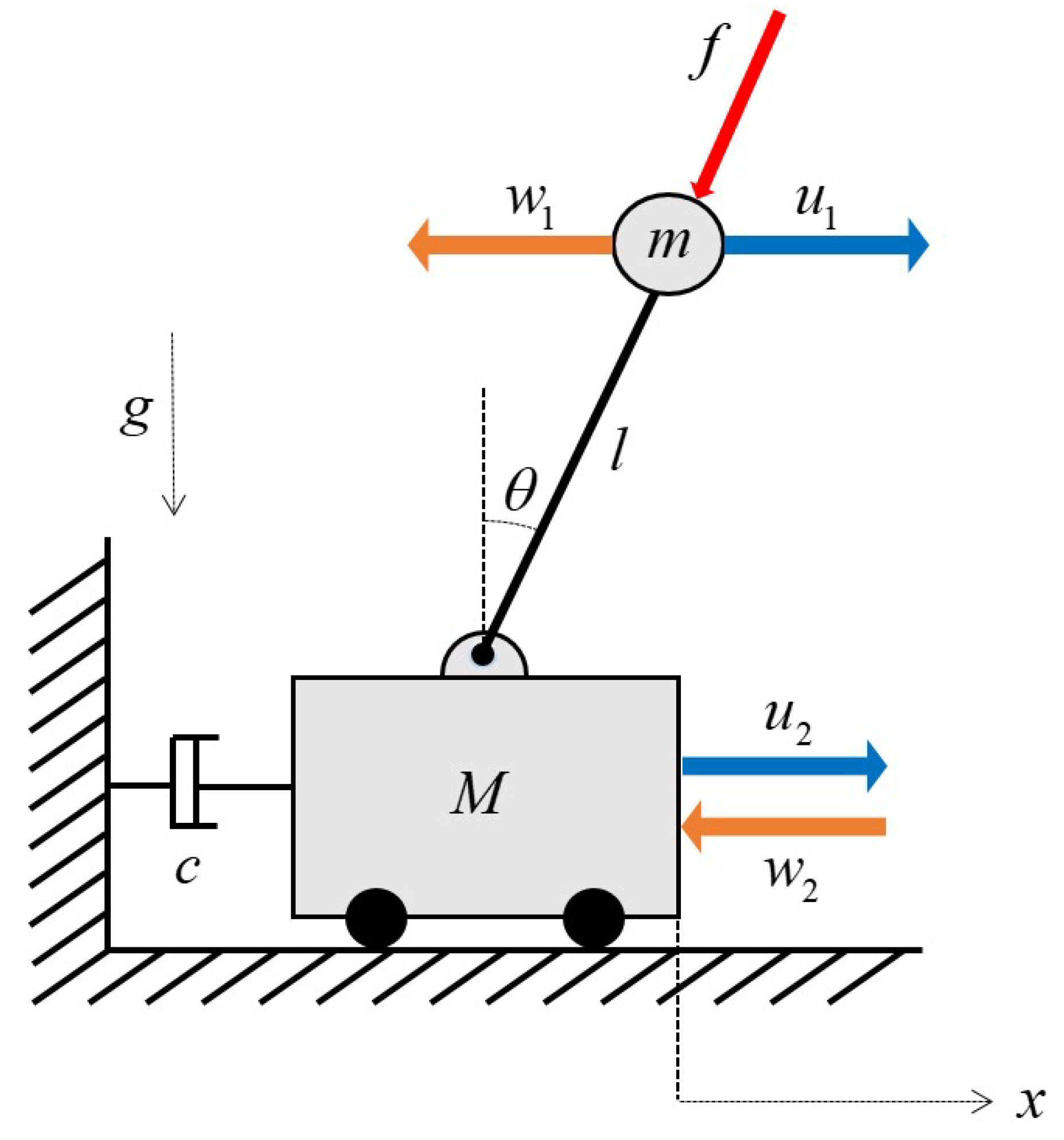
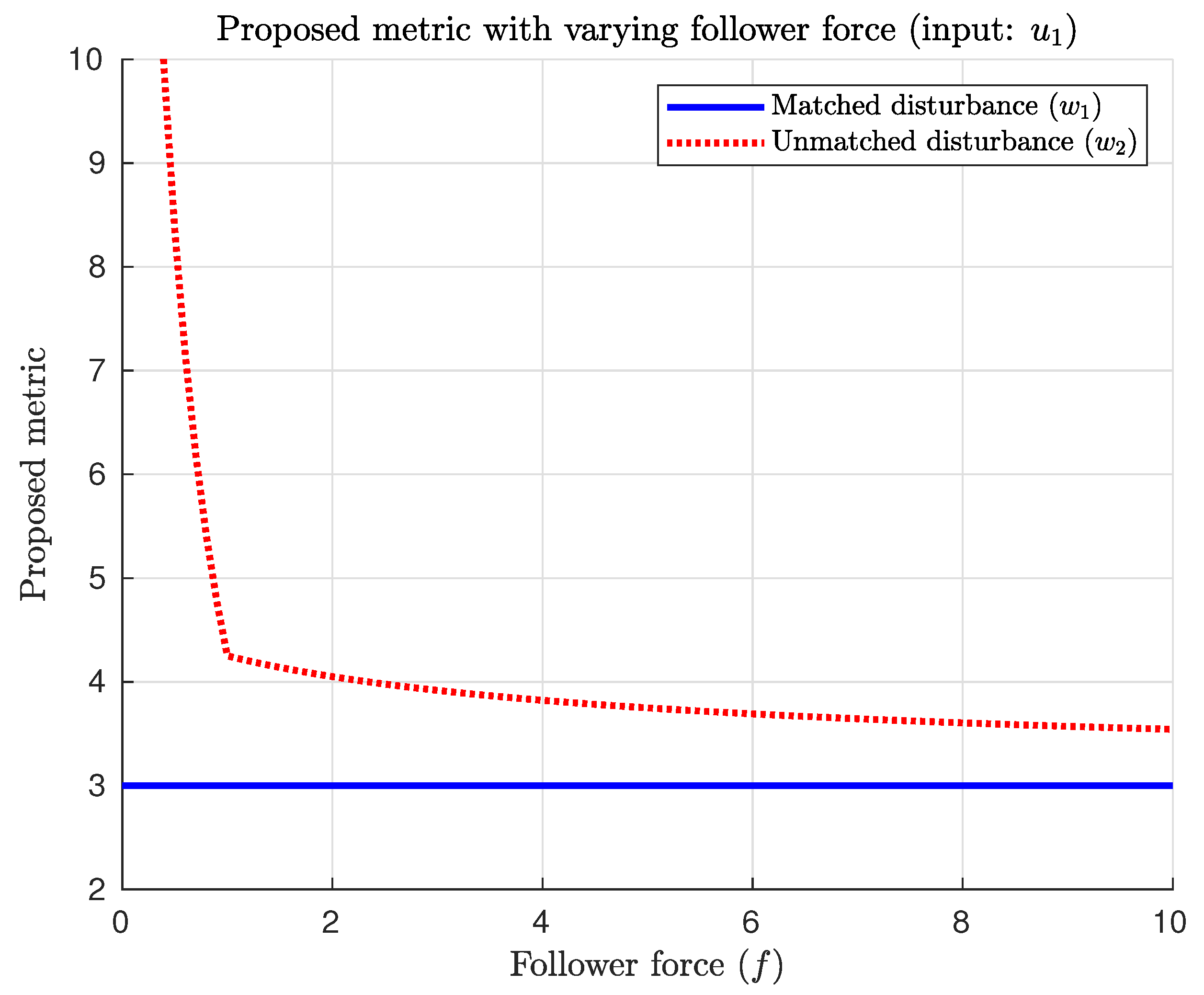
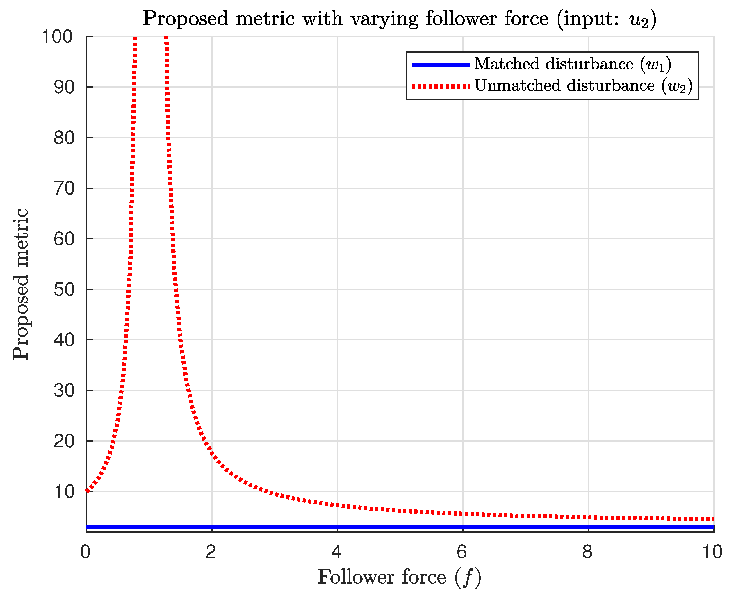
4.1. Inverted Pendulum–Cart System

A simple inverted pendulum–cart system is illustrated in Figure 1. The system has two input variables, $u_1$ and $u_2$, which are the forces in the horizontal direction applied to the end of the pendulum and the cart, respectively. There are also two disturbance variables, $w_1$ and $w_2$, which are the unexpected external forces applied to the end of the pendulum and the cart, respectively. The linearized model for the system can be represented as the following state-space equation:

$$\begin{array}{cc}\hfill \dot{x}\left(t\right)=Ax\left(t\right)& +B_1{u}_1\left(t\right)+B_2{u}_2\left(t\right)\hfill \\ \hfill & +D_1{w}_1\left(t\right)+D_2{w}_2\left(t\right)\hfill \end{array}$$

(91)

The state and matrices are given by

$$\begin{array}{cc}\hfill x\left(t\right)=\left[\begin{array}{c}v\left(t\right)\\ \theta \left(t\right)\\ \dot{\theta }\left(t\right)\end{array}\right]& ,A=\left[\begin{array}{ccc}-{\displaystyle \frac{c}{M}}& -{\displaystyle \frac{mg+f}{M}}& 0\\ 0& 0& 1\\ {\displaystyle \frac{c}{Ml}}& {\displaystyle \frac{g}{l}}\left({\displaystyle \frac{m}{M}}+1\right)& 0\end{array}\right],\hfill \\ \hfill B_1& =\left[\begin{array}{c}0\\ 0\\ -{\displaystyle \frac{1}{ml}}\end{array}\right],B_2=\left[\begin{array}{c}{\displaystyle \frac{1}{M}}\\ 0\\ -{\displaystyle \frac{1}{Ml}}\end{array}\right],\hfill \\ \hfill & D_1=-B_1,D_2=-B_2\hfill \end{array}$$

(92)

where M and m denote the mass of the cart and end of the pendulum, respectively, and g denotes the gravitational acceleration, l denotes the length of the pendulum, c denotes the damping coefficient, v denotes the velocity of the cart ($v=\dot{x}$), and $\theta$ denotes the angle of the pendulum. Additionally, f denotes the follower force that is applied to the end of the pendulum, directed toward the hinge. For simplicity, all parameters in Equation (92), except the follower force f, are set to 1 for the following demonstrations, including the variances of the disturbances.

The proposed metric was computed in two cases: with and without the follower force. The follower force was set to 0 for the first case. Then, the matrices in Equation (92) were rewritten as

$$A=\left[\begin{array}{ccc}-1& -1& 0\\ 0& 0& 1\\ 1& 2& 0\end{array}\right],B_1=\left[\begin{array}{c}0\\ 0\\ -1\end{array}\right],B_2=\left[\begin{array}{c}1\\ 0\\ -1\end{array}\right]$$

(93)

The decoupled state-space form represented in Equation (12) can be obtained by the following linear transformation using an eigenvalue decomposition of the system matrix in Equation (93):

$$\begin{array}{c}\hfill {\displaystyle \frac{d}{dt}}\left\{T^{-1}\left[\begin{array}{c}v\\ \theta \\ \dot{\theta }\end{array}\right]\right\}=\left[\begin{array}{cc}{A}_s& 0\\ 0& A_a\end{array}\right]\left\{T^{-1}\left[\begin{array}{c}v\\ \theta \\ \dot{\theta }\end{array}\right]\right\}\\ \hfill +\left(T^{-1}{B}_1\right)u_1+\left(T^{-1}{B}_2\right)u_2\end{array}$$

(94)

where

$$\begin{array}{cc}\hfill T& =\left[\begin{array}{ccc}0.5177& -0.8547& 0.2682\\ 0.4152& 0.4743& -0.6027\\ -0.7481& -0.2111& -0.7515\end{array}\right],\hfill \\ \hfill A_s& =\left[\begin{array}{cc}-1.8019& 0\\ 0& -0.4450\end{array}\right],A_a=1.2470\hfill \end{array}$$

(95)

The proposed metric can be computed by substituting the decoupled state-space forms of Equations (94) and (95) into Equation (73).

The computation results are presented in

Table 1. Computation results of the proposed metric for different input and disturbance combinations.

Inputs	${\mathit{w}}_1$	${\mathit{w}}_2$
$u_1$	3.00	22.20
$u_2$	9.99	3.00

. It can be observed that the proposed metric yielded the smallest value when the input and disturbance locations are identical, i.e., satisfying the matched disturbance condition. This result indicates that the disturbance could be rejected with the least input energy when it satisfied the matched condition, which is a reasonable result and is consistent with the result for asymptotically stable systems [22]. For unmatched disturbance cases, the result suggests that using $u_2$ was more efficient than using $u_1$, which was an intuitive and reasonable outcome since the force applied to the end of the pendulum cannot directly affect the velocity of the cart, as represented in $B_1$ of Equation (92). Therefore, it could be confirmed that the metric was not only applicable to unstable systems but also provided physically correct information for actuator allocation.

In order to investigate the properties of the proposed metric further, the metric was computed for the case where the follower force was present, which is the second case of this example. Figure 2 and Figure 3 illustrate the computation results of the proposed metric for the inputs $u_1$ and $u_2$, respectively, while varying the follower force. Figure 2 shows that the metric for $u_1$ with the unmatched disturbance decreased as the follower force increased, and it converged to that with the matched disturbance. This was because increasing the follower force had the same effect as having the system composed of one rigid body, which allowed the unmatched disturbance to be treated as a matched disturbance. This behavior is similar to the large stiffness case for a mass–spring–damper system introduced by Kang et al. [22], where the unmatched disturbance can also be regarded as a matched disturbance under a high stiffness condition.

Figure 3 shows that the metric for $u_2$ under unmatched conditions also converged to that under the matched condition as the follower force increased. However, as the follower force approached 1, the metric exhibited a sharp increase, indicating that the disturbance could not be rejected with finite input energy. This is related to the controllability of the system. The system and input matrices for $f=1$ are given by

$$A=\left[\begin{array}{ccc}-1& -2& 0\\ 0& 0& 1\\ 1& 2& 0\end{array}\right],B_2=\left[\begin{array}{c}1\\ 0\\ -1\end{array}\right]$$

(96)

The controllability matrix was not a full-rank matrix with the matrices in Equation (96), which means that the system was uncontrollable. Nonetheless, the proposed metric under the matched condition for $f=1$ still yielded a finite value, regardless of the controllability. This implies that although the system could not fully control all states, it could still reject the matched disturbance. This finding is also consistent with the results of previous studies on asymptotically stable systems [22]. All these results in this example demonstrate that the proposed metric preserves physically meaningful properties of the DoDR.

One point worth noting in this example is that there were no numerical issues in calculating the proposed metric. As previously mentioned, the controllability Gramian matrix of an unstable system diverges over time, causing numerical problems when computing the inverse matrix to calculate the existing time-dependent metric [22,25,26,27]. This problem can be observed from Figure 4, which illustrates the reciprocal of the condition number (RCN) of the controllability Gramian for the input $u_2$ and the corresponding DoDR computation results under the disturbance $w_1$. As shown in the figure, the RCN of the controllability Gramian obtained from the differential equation was significantly smaller compared with that computed from the proposed steady-state solution, which caused the numerical problem when computing the inverse of the controllability Gramian. Due to this numerical problem, an accurate calculation of the DoDR was not possible with the existing method, as shown in the computation results. These results show that the proposed metric was more suitable for application to unstable systems, not only because of its low computation burden but also accurate calculation without such numerical issues.

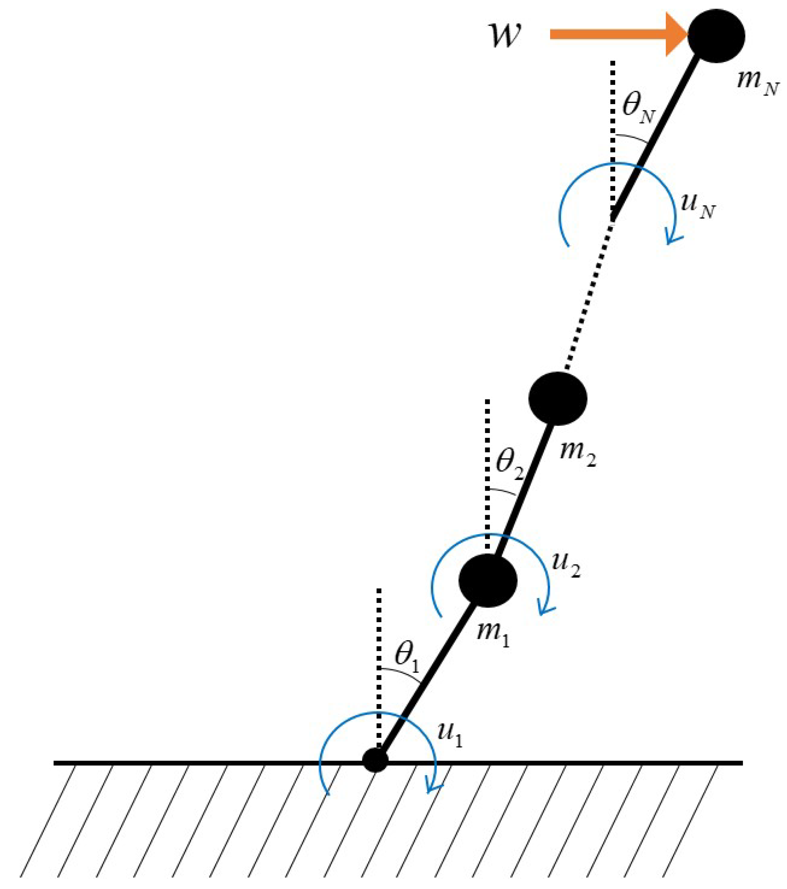
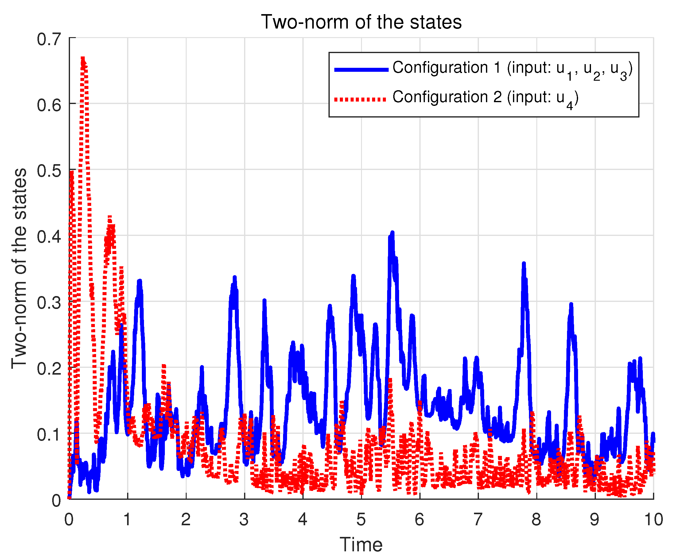
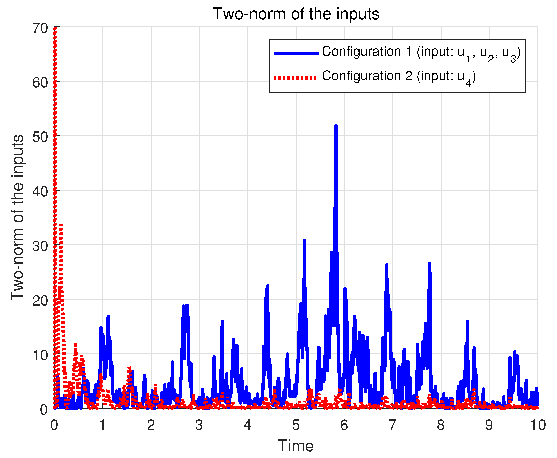
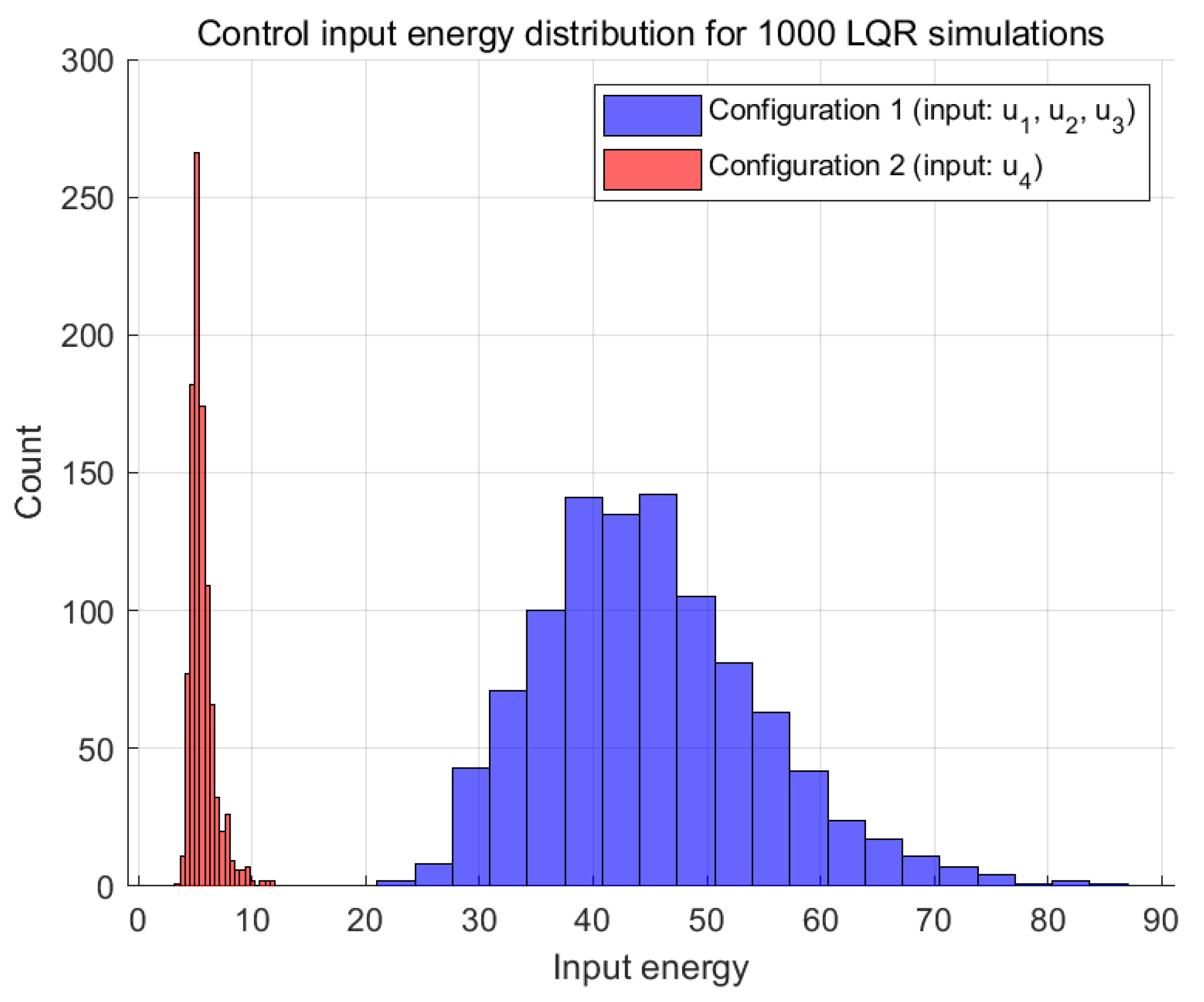
4.2. Multi-Link Inverted Pendulum System

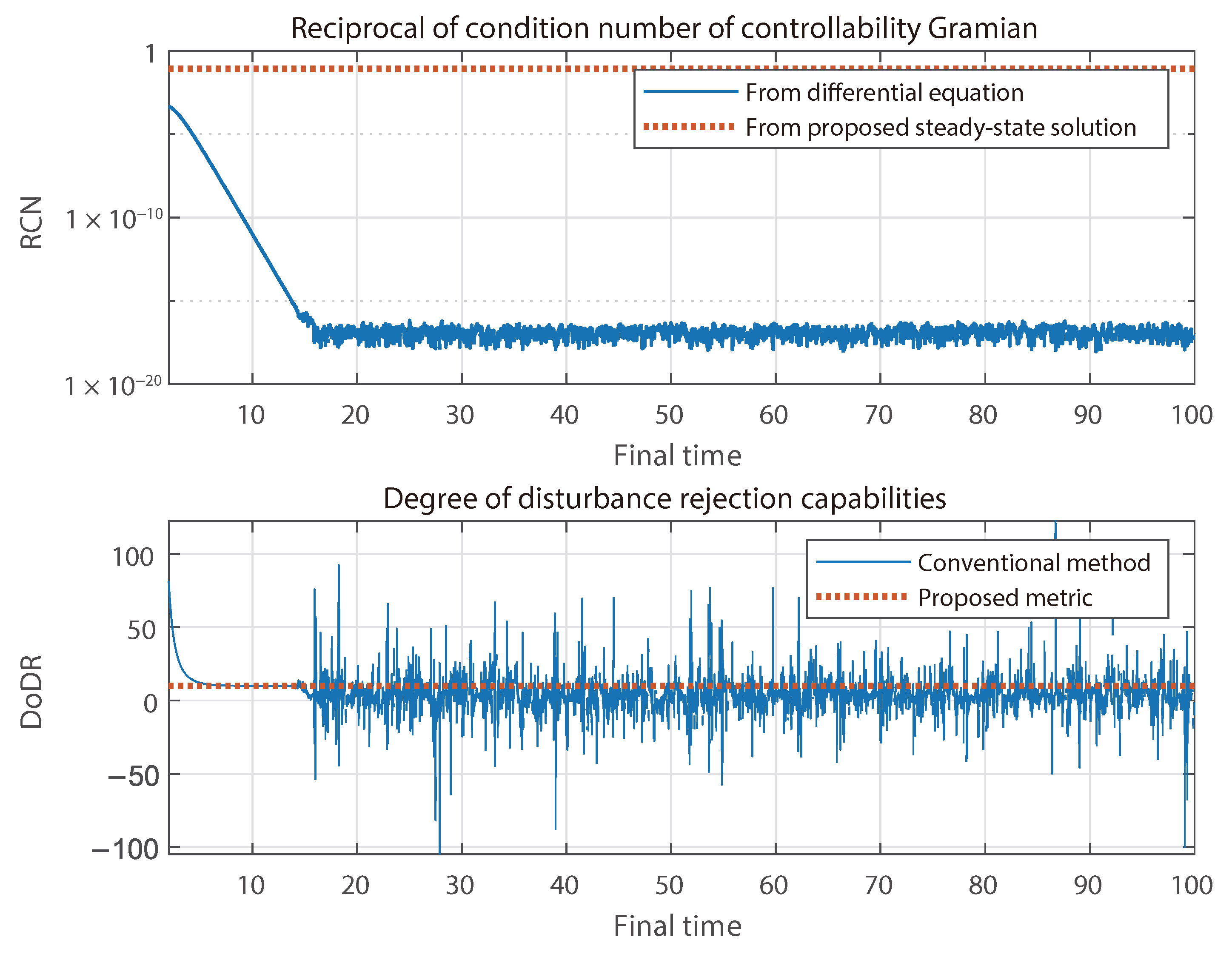
An input selection problem for a multi-link inverted pendulum system, often used as the model for human upright stance [42,43], was demonstrated in this example. The system model for this example is illustrated in Figure 5. The state-space equation for the system with an arbitrary number of links N is given by [44]:

$$\dot{x}=Ax+\mathbf{B}\mathbf{u}+Dw$$

(97)

where the state and inputs are defined as

$$\begin{array}{cc}\hfill & x={\left[\begin{array}{cccccc}{\theta }_1& \cdots & {\theta }_N& {\dot{\theta }}_1& \cdots & {\dot{\theta }}_N\end{array}\right]}^T\hfill \\ \hfill & \mathbf{u}={\left[\begin{array}{ccc}{u}_1& \cdots & u_N\end{array}\right]}^T\hfill \end{array}$$

(98)

and the matrices are written as

$$\begin{array}{cc}\hfill & A=\left[\begin{array}{cc}0& I\\ {\left(M_N{L}_N\right)}^{-1}{M}_a& 0\end{array}\right]\hfill \\ \hfill & \mathbf{B}=\left[\begin{array}{ccc}{B}_1& \cdots & B_N\end{array}\right]=\left[\begin{array}{c}0\\ {\left(M_N{L}_N\right)}^{-1}{M}_b\end{array}\right]\hfill \\ \hfill & D=\left[\begin{array}{c}0\\ {\left(M_N{L}_N\right)}^{-1}{M}_d\end{array}\right]\hfill \end{array}$$

(99)

$$\begin{array}{cc}\hfill & M_a=\mathrm{diag}\left(\begin{array}{cccc}g\sum _{i=1}^N{m}_i,& g\sum _{i=2}^N{m}_i,& \cdots & m_{N}g\end{array}\right)\hfill \\ \hfill & M_b=\mathrm{diag}\left(\begin{array}{cccc}1/l_1,& 1/l_2,& \cdots & 1/l_N\end{array}\right)\hfill \\ \hfill & M_d=\mathrm{diag}\left(\begin{array}{cccc}0,& \cdots & 0,& 1\end{array}\right)\hfill \end{array}$$

(100)

$$\begin{array}{cc}\hfill & M_N=\left[\begin{array}{cccc}{m}_1& m_2& \cdots & m_N\\ 0& m_2& \cdots & m_N\\ ⋮& ⋮& \ddots & ⋮\\ 0& 0& \cdots & m_N\end{array}\right]\hfill \\ \hfill & L_N=\left[\begin{array}{cccc}{l}_1& 0& \cdots & 0\\ l_1& l_2& \cdots & 0\\ l_1& ⋮& \ddots & ⋮\\ l_1& l_2& \cdots & l_N\end{array}\right]\hfill \end{array}$$

(101)

where ${\theta }_i$, $u_i$, $m_i$, and $l_i$ denote the angle, input torque, mass, and length of the i-th pendulum, respectively; w denotes a disturbance force applied to the end of the pendulum; and $B_i$ denotes the input matrix for the input $u_i$. In this example, the number of links N was set to 4, and $m_i$ and $l_i$ for all i were set to 1 for the sake of simplicity. The variance of the disturbance was also set to 1. Similarly to the first example, the decoupled form in Equation (12) could also be obtained by eigenvalue decomposition, which is omitted for brevity.

The computation results of the proposed metric for all the control configurations are presented in

Table 2. Computation results of the proposed metric for different input selections.

# of Actuators	Input Selected				Proposed Metric
	${\mathit{u}}_{\mathbf{1}}$	${\mathit{u}}_{\mathbf{2}}$	${\mathit{u}}_{\mathbf{3}}$	${\mathit{u}}_{\mathbf{4}}$
1	O				5.49 × ${10}^4$
		O			1.55 × ${10}^5$
			O		1.07 × ${10}^5$
				O	8.00 × ${10}^0$
2	O	O			2.56 × ${10}^3$
	O		O		4.25 × ${10}^2$
	O			O	4.14 × ${10}^0$
		O	O		2.47 × ${10}^2$
		O		O	4.19 × ${10}^0$
			O	O	2.95 × ${10}^0$
3	O	O	O		1.14 × ${10}^2$
	O	O		O	3.28 × ${10}^0$
	O		O	O	2.43 × ${10}^0$
		O	O	O	2.34 × ${10}^0$
4	O	O	O	O	2.15 × ${10}^0$

. The results show that using $u_4$ was the most efficient control configuration regardless of the number of actuators used. This was because, similar to the previous example, $u_4$ was the input that satisfied the matched condition. Although the table shows a trend in which the proposed metric decreased as the number of actuators increased, it also presents that using $u_4$ as the only input showed a better disturbance rejection capability than using all the other actuators.

To verify the result, control simulations were performed for two control configurations: configuration 1 used three inputs ($u_1$, $u_2$, and $u_3$) and configuration 2 used $u_4$ as the only input. Since the proposed metric was independent of the controller design, and the DoDR metric is known to predict the performance of control systems with a high degree of accuracy regardless of the type of controller [22,27,38], a linear quadratic regulator (LQR) was applied in this control simulation. The weighting matrices of the LQR for states and inputs were set to identity matrices, and the disturbance force was assumed to be GWN. The two-norm of the controlled states and the control inputs for each case over time are shown in Figure 6 and Figure 7, respectively. As represented in the figures, configuration 2 showed a better control performance with lower input energy, except for the transient region around the time for 0 to 1. This result indicates that configuration 2 was better suited for persistently rejecting the disturbance force over long periods of time, despite using only one actuator. Since the proposed metric is defined for the steady-state condition, this result demonstrates that the metric quantifies the disturbance rejection capabilities of unstable systems well.

In order to confirm that the obtained results were not specific to a particular case, 1000 more simulations were performed with different disturbance forces, whose results are shown in Figure 8 and Figure 9. The figures show the distribution for the energies of the states and inputs within the time interval 1 to 10, which excluded the transient region. As with the results in Figure 6 and Figure 7, the distribution of the energies also indicate that configuration 2 outperformed configuration 1 in most simulation cases. Consequently, all these simulation results collectively demonstrate that the proposed metric enabled quite accurate input selection.

4.3. Discussion

This subsection examines the numerical examples demonstrated earlier and explains how the proposed metric outperformed the the DoDR metric suggested in previous studies. In the first example involving the inverted pendulum–cart system, the DoDR values were compared between those calculated using the steady-state solution derived in this study and those obtained using the time-dependent metric from previous studies. As observed in Figure 4, the method from previous studies resulted in the divergence of the controllability Gramian, which led to a very high RCN. This divergence prevented the accurate computation of the inverse of the controllability Gramian matrix, which caused the DoDR value to vary depending on the final time. This variation was purely a numerical issue, which should not occur under identical system conditions. In other words, using the conventional method failed to accurately predict the disturbance rejection capabilities of unstable systems, which made it impossible to determine the optimal actuator placement for disturbance rejection. For example, as shown in Figure 4, the DoDR values calculated for the unmatched disturbance case using the conventional method could sometimes be smaller than 3.00, which was the value for the matched disturbance case. This could lead to selecting an incorrect input that did not satisfy the matched disturbance, which produced erroneous results. Therefore, the proposed metric was not only computationally more efficient for unstable systems but also allowed for a more accurate disturbance rejection system design.

While the first example verified that the proposed metric accurately evaluated the disturbance rejection capabilities, the second example tested whether using the input selected based on the proposed metric was more effective for disturbance control compared with other inputs. The optimal input selected was $u_4$, and it was confirmed through 1000 simulations that this input was more effective for disturbance control than using all of the other inputs ($u_1$, $u_2$, $u_3$). Although previous studies also showed that the input selected using the DoDR was the most effective for disturbance rejection [26,27,38], these metrics were applicable only to systems without unstable modes and were validated solely for systems with stable or undamped modes. In contrast, the proposed metric not only facilitates efficient and accurate calculations for unstable systems but also effectively predicts disturbance rejection performance for such systems, as confirmed through the control simulations conducted in this study.

5. Conclusions

This paper introduces a Gramian-based metric for quantifying the disturbance rejection capabilities of linear unstable systems. The proposed metric is defined as the steady-state solution of the degree of disturbance rejection (DoDR) and is derived by leveraging the properties of the Gramian matrices for unstable systems, which are also rigorously proved in this paper. The metric computation involves solving only four algebraic equations, eliminating the numerical issues associated with time-dependent solutions and diverging Gramian matrices. This characteristic ensures computational efficiency and applicability to unstable systems.

The numerical examples presented in this study highlighted the key advantages of the proposed metric. For instance, in the inverted pendulum–cart system example, the proposed metric demonstrated its ability to provide consistent and accurate evaluations of disturbance rejection capabilities, even when the controllability Gramian diverged. This addresses a significant limitation of previously proposed DoDR metrics, which often led to numerical inconsistencies and unreliable results due to dependency on the final time and sensitivity to divergence. Moreover, the proposed metric was shown to facilitate the identification of optimal input configurations for disturbance rejection. In simulations that involved the second example system, the metric successfully identified the optimal input that yielded a superior disturbance control performance compared with all other possible input combinations. This result highlighted the practical utility of the proposed metric in developing effective disturbance control systems for unstable systems.

The proposed metric addresses the limitations of existing metrics and extends its applicability to unstable systems, enabling the following future research directions:

• Robust control system design for multi-input systems: By leveraging the metric’s independence from the controller design, it is possible to evaluate the disturbance rejection performance prior to designing the controller and incorporate the results into the system design. This can be particularly useful in applications such as the optimal input allocation for over-actuated vehicles [45] or multi-rotor aerial vehicles [31,32,33], as well as in fault-tolerant control system design [46,47].
• Extension to nonlinear systems: Similar to how conventional Gramian-based DoC metrics have been extended from linear to nonlinear systems [9,10,11,12], the main theorems derived in this study can be utilized to adapt the proposed metric for nonlinear systems. Such an extension would allow for its application in the control system design of representative nonlinear systems, such as walking robots [34,35,36].

References

1. Paige, C. Properties of numerical algorithms related to computing controllability. IEEE Trans. Autom. Control 1981, 26, 130–138. [Google Scholar] [CrossRef]
2. Hughes, P.; Skelton, R. Controllability and observability of linear matrix-second-order systems. J. Appl. Mech. 1980, 47, 415–420. [Google Scholar] [CrossRef]
3. Hamdan, A.; Nayfeh, A. Measures of modal controllability and observability for first-and second-order linear systems. J. Guid. Control. Dyn. 1989, 12, 421–428. [Google Scholar] [CrossRef]
4. Tarokh, M. Measures for controllability, observability and fixed modes. IEEE Trans. Autom. Control 1992, 37, 1268–1273. [Google Scholar] [CrossRef]
5. Viswanathan, C.; Longman, R.; Likins, P. A degree of controllability definition-fundamental concepts and application to modal systems. J. Guid. Control. Dyn. 1984, 7, 222–230. [Google Scholar] [CrossRef]
6. Müller, P.; Weber, H. Analysis and optimization of certain qualities of controllability and observability for linear dynamical systems. Automatica 1972, 8, 237–246. [Google Scholar] [CrossRef]
7. Marx, B.; Koenig, D.; Georges, D. Optimal sensor/actuator location for descriptor systems using Lyapunov-like equations. In Proceedings of the 41st IEEE Conference on Decision and Control, Las Vegas, NV, USA, 10–13 December 2002; Volume 4, pp. 4541–4542. [Google Scholar]
8. Marx, B.; Koenig, D.; Georges, D. Optimal sensor and actuator location for descriptor systems using generalized gramians and balanced realizations. In Proceedings of the 2004 American Control Conference, Boston, MA, USA, 30 June–2 July 2004; Volume 3, pp. 2729–2734. [Google Scholar]
9. Singh, A.K.; Hahn, J. Determining optimal sensor locations for state and parameter estimation for stable nonlinear systems. Ind. Eng. Chem. Res. 2005, 44, 5645–5659. [Google Scholar] [CrossRef]
10. Singh, A.K.; Hahn, J. Sensor location for stable nonlinear dynamic systems: Multiple sensor case. Ind. Eng. Chem. Res. 2006, 45, 3615–3623. [Google Scholar] [CrossRef]
11. Shaker, H.R.; Stoustrup, J. An interaction measure for control configuration selection for multivariable bilinear systems. Nonlinear Dyn. 2013, 72, 165–174. [Google Scholar] [CrossRef]
12. Tahavori, M. Model reduction via truncated cross-gramian for bilinear systems. In Proceedings of the 2021 International Conference on Recent Advances in Mathematics and Informatics (ICRAMI), Tebessa, Algeria, 21–22 September 2021; pp. 1–5. [Google Scholar]
13. Zhao, S.; Pasqualetti, F. Networks with diagonal controllability Gramian: Analysis, graphical conditions, and design algorithms. Automatica 2019, 102, 10–18. [Google Scholar] [CrossRef]
14. Babazadeh, M. Gramian-based vulnerability analysis of dynamic networks. IET Control Theory Appl. 2022, 16, 625–637. [Google Scholar] [CrossRef]
15. Hać, A.; Liu, L. Sensor and actuator location in motion control of flexible structures. J. Sound Vib. 1993, 167, 239–261. [Google Scholar] [CrossRef]
16. Roh, H.S.; Park, Y. Actuator and exciter placement for flexible structures. J. Guid. Control. Dyn. 1997, 20, 850–856. [Google Scholar] [CrossRef]
17. Shaker, H.R.; Tahavori, M. Optimal sensor and actuator location for unstable systems. J. Vib. Control 2013, 19, 1915–1920. [Google Scholar] [CrossRef]
18. Seyed Sakha, M.; Shaker, H.R.; Tahavori, M. Optimal sensors and actuators placement for large-scale switched systems. Int. J. Dyn. Control 2019, 7, 147–156. [Google Scholar] [CrossRef]
19. Hovd, M.; Skogestad, S. Simple frequency-dependent tools for control system analysis, structure selection and design. Automatica 1992, 28, 989–996. [Google Scholar] [CrossRef]
20. Cao, Y.; Rossiter, D.; Owens, D. Input selection for disturbance rejection under manipulated variable constraints. Comput. Chem. Eng. 1997, 21, S403–S408. [Google Scholar] [CrossRef]
21. Mirza, M.A.; Van Niekerk, J.L. Optimal actuator placement for active vibration control with known disturbances. J. Vib. Control 1999, 5, 709–724. [Google Scholar] [CrossRef]
22. Kang, O.; Park, Y.; Park, Y.; Suh, M. New measure representing degree of controllability for disturbance rejection. J. Guid. Control. Dyn. 2009, 32, 1658–1661. [Google Scholar] [CrossRef]
23. Lee, H.; Park, Y. Degree of disturbance rejection capability for linear anti-stable systems. In Proceedings of the 2014 14th International Conference on Control, Automation and Systems (ICCAS 2014), Seoul, Republic of Korea, 22–25 October 2014; pp. 154–156. [Google Scholar]
24. Lee, H.; Park, Y. Degree of disturbance rejection capability for linear marginally stable systems. In Proceedings of the 2015 15th International Conference on Control, Automation and Systems (ICCAS), Busan, Republic of Korea, 13–16 October 2015; pp. 307–310. [Google Scholar]
25. Xia, Y.; Yin, M.; Cai, C.; Zhang, B.; Zou, Y. A new measure of the degree of controllability for linear system with external disturbance and its application to wind turbines. J. Vib. Control 2018, 24, 739–759. [Google Scholar] [CrossRef]
26. Xia, Y.; Yin, M.; Li, R.; Liu, D.; Zou, Y. Integrated structure and maximum power point tracking control design for wind turbines based on degree of controllability. J. Vib. Control 2019, 25, 397–407. [Google Scholar] [CrossRef]
27. Xia, Y.; Li, R.; Yin, M.; Zou, Y. A quantitative measure of the degree of output controllability for output regulation control systems: Concept, approach, and applications. J. Vib. Control 2022, 28, 2803–2815. [Google Scholar] [CrossRef]
28. Jeong, I.; Park, Y. Input energy minimization with acoustic potential energy constraint for active noise control system. J. Vib. Control 2024, 2024, 10775463241227477. [Google Scholar] [CrossRef]
29. Zhou, K.; Salomon, G.; Wu, E. Balanced realization and model reduction for unstable systems. Int. J. Robust Nonlinear Control. IFAC-Affil. J. 1999, 9, 183–198. [Google Scholar] [CrossRef]
30. Lee, H.; Park, Y. Degree of controllability for linear unstable systems. J. Vib. Control 2016, 22, 1928–1934. [Google Scholar] [CrossRef]
31. Chang, X.; Jin, C.; Cheng, Y. Dynamics and advanced active disturbance rejection control of tethered UAV. Appl. Math. Model. 2024, 135, 640–665. [Google Scholar] [CrossRef]
32. Khadraoui, S.; Fareh, R.; Baziyad, M.; Elbeltagy, M.B.; Bettayeb, M. A Comprehensive Review and Applications of Active Disturbance Rejection Control for Unmanned Aerial Vehicles. IEEE Access 2024, 12, 185851–185868. [Google Scholar] [CrossRef]
33. Le, W.; Xie, P.; Chen, J. Disturbance rejection control of the agricultural quadrotor based on adaptive neural network. Inf. Process. Agric. 2024. In Press. [Google Scholar] [CrossRef]
34. Espinosa-Espejel, K.I.; Rosales-Luengas, Y.; Salazar, S.; Lopéz-Gutiérrez, R.; Lozano, R. Active Disturbance Rejection Control via Neural Networks for a Lower-Limb Exoskeleton. Sensors 2024, 24, 6546. [Google Scholar] [CrossRef] [PubMed]
35. Kang, J.; Kim, H.b.; Ham, B.I.; Kim, K.S. External Force Adaptive Control in Legged Robots Through Footstep Optimization and Disturbance Feedback. IEEE Access 2024, 12, 157531–157539. [Google Scholar] [CrossRef]
36. Zhao, J.; Zhang, Y.; Hou, H.; Yue, Y.; Meng, K.; Yang, Z. Active Disturbance Rejection Control With Backstepping for Decoupling Control of Hydraulic Driven Lower Limb Exoskeleton Robot. IEEE Trans. Ind. Electron. 2024, 72, 714–723. [Google Scholar] [CrossRef]
37. Shen, M.; Gu, Y.; Zhu, S.; Zong, G.; Zhao, X. Mismatched quantized H output-feedback control of fuzzy Markov jump systems with a dynamic guaranteed cost triggering scheme. IEEE Trans. Fuzzy Syst. 2023, 32, 1681–1692. [Google Scholar] [CrossRef]
38. Lee, H. Controllability measure for disturbance rejection capabilities of control systems with undamped flexible structures. J. Frankl. Inst. 2024, 361, 107320. [Google Scholar] [CrossRef]
39. Bandyopadhyay, B.; Deepak, F.; Kim, K.S. Sliding Mode Control Using Novel Sliding Surfaces; Springer Science & Business Media: Berlin/Heidelberg, Germany, 2009; Volume 392. [Google Scholar]
40. Tao, G. Adaptive Control Design and Analysis; John Wiley & Sons: Hoboken, NJ, USA, 2003; Volume 37. [Google Scholar]
41. Chen, B.M.; Lin, Z.; Shamash, Y. Linear Systems Theory: A Structural Decomposition Approach; Springer Science & Business Media: Berlin/Heidelberg, Germany, 2004. [Google Scholar]
42. Colobert, B.; Crétual, A.; Allard, P.; Delamarche, P. Force-plate based computation of ankle and hip strategies from double-inverted pendulum model. Clin. Biomech. 2006, 21, 427–434. [Google Scholar] [CrossRef]
43. Günther, M.; Grimmer, S.; Siebert, T.; Blickhan, R. All leg joints contribute to quiet human stance: A mechanical analysis. J. Biomech. 2009, 42, 2739–2746. [Google Scholar] [CrossRef]
44. Bowden, C.; Holderbaum, W.; Becerra, V. Actuator placement in the multi-link inverted pendulum. In Proceedings of the UKACC International Conference on Control 2010, Coventry, UK, 7–10 September 2010; pp. 1–6. [Google Scholar]
45. Park, J.; Park, Y. Optimal input design for fault identification of overactuated electric ground vehicles. IEEE Trans. Veh. Technol. 2015, 65, 1912–1923. [Google Scholar] [CrossRef]
46. Park, J.; Park, Y. Experimental Verification of Fault Identification for Overactuated System With a Scaled-Down Electric Vehicle. Int. J. Automot. Technol. 2020, 21, 1037–1045. [Google Scholar] [CrossRef]
47. Park, J.; Park, Y. Multiple-Actuator Fault Isolation Using a Minimal 1-Norm Solution with Applications in Overactuated Electric Vehicles. Sensors 2022, 22, 2144. [Google Scholar] [CrossRef] [PubMed]
Figure 1. Inverted pendulum–cart under a follower force.
Mathematics 13 00006 g001
Figure 2. Proposed metric for input u 1 under varying follower force.
Mathematics 13 00006 g002
Figure 3. Proposed metric for input u 2 under varying follower force.
Mathematics 13 00006 g003
Figure 4. RCN of the controllability Gramian (top) and the DoDR computation results (bottom).
Mathematics 13 00006 g004
Figure 5. Multi-link inverted pendulum.
Mathematics 13 00006 g005
Figure 6. Two-norm of the states controlled with an LQR.
Mathematics 13 00006 g006
Figure 7. Two-norm of the control inputs for an LQR.
Mathematics 13 00006 g007
Figure 8. Controlled state energy distribution for 1000 LQR simulations.
Mathematics 13 00006 g008
Figure 9. Controlled input energy distribution for 1000 LQR simulations.
Mathematics 13 00006 g009