Abstract
In this paper, we explore the connection between sensor networks and graph theory. Sensor networks represent distributed systems of interconnected devices that collect and transmit data, while graph theory provides a robust framework for modeling and analyzing complex networks. Specifically, we focus on vertex coloring, Eulerian paths, and Hamiltonian paths within the Delaunay graph associated with a sensor network. These concepts have critical applications in sensor networks, including connectivity analysis, efficient data collection, route optimization, task scheduling, and resource management. We derive theoretical results related to the chromatic number and the existence of Eulerian and Hamiltonian trails in the graph linked to the sensor network. Additionally, we complement this theoretical study with the implementation of several algorithmic procedures. A case study involving the monitoring of a sugarcane field, coupled with a computational analysis, demonstrates the performance and practical applicability of these algorithms in real-world scenarios.
MSC:
52-04; 05C22; 68M15; 90C35
1. Introduction
One of the most stimulating areas of research today across science, engineering, and particularly mathematics involves identifying and studying novel connections between disciplines. Such interdisciplinary approaches enable researchers to address open problems, refine existing theories, and uncover new insights.
This paper explores the intersection of graph theory and sensor networks. Sensor networks, comprising distributed systems of interconnected devices that collect and transmit data, represent a dynamic technological domain. Graph theory, in turn, provides a powerful framework for modeling and analyzing these complex systems. By leveraging graph theory, researchers have achieved significant advancements in understanding, optimizing, and managing sensor networks.
In the context of the modern interconnected landscape, sensor networks play a crucial role pivotal in real-time data collection and transmission. Modeling these systems as graphs creates a synergy that facilitates efficient analysis, optimization, and management of network connectivity and information flow.
Graph theory has already proven its utility in various fields, including sensor networks. For example, in [1] the authors study several graph-based optimization approaches such as node placement, routing protocols, and data aggregation to minimize energy consumption and extend network lifespan. Other studies employ graph algorithms for topology construction, energy-efficient communication, and operations optimization in wireless sensor networks [2]. Similarly, graph-based methods address challenges such as load balancing and connectivity [3,4,5].
This paper explores three fundamental concepts in graph theory: vertex coloring, Eulerian paths, and Hamiltonian paths and their practical applications in sensor networks. These tools have proven utility in tasks such as connectivity analysis, route optimization, task scheduling, resource management, and data collection. For instance, Eulerian cycles have been applied to optimize transportation routes [6], Hamiltonian paths have been used to design energy-efficient mobile charging mechanisms [7], and vertex coloring has been utilized to assign roles or tasks within sensor networks [8].
The main objective of this study is to advance the understanding and application of graph-based methods for improving the efficiency and robustness of sensor network management. Specifically, we aim to associate sensor networks with Delaunay graphs to analyze their structural and functional properties through three key graph tools: Eulerian trails, Hamiltonian paths, and chromatic numbers. While Hamiltonian paths in Delaunay graphs have been studied extensively under specific conditions, such as the -metric [9], this work tackles several open questions related to Delaunay graphs. One key focus is the Eulerian nature of these graphs, investigating whether they can be classified as Eulerian or semi-Eulerian and under what specific conditions this classification holds. Another aspect explored is the chromatic number of Delaunay graphs, aiming to determine its bounds or exact values. Finally, this study examines the practical implications of these theoretical findings, particularly in enhancing the connectivity, efficiency, and energy management of sensor networks in real-world applications.
To address these objectives, Section 4 provides new theoretical results regarding Eulerian paths, Hamiltonian paths, and vertex coloring in Delaunay Graphs. These results are complemented by the implementation of novel algorithmic methods designed to leverage these graph tools effectively. Finally, we present a case study involving the monitorization of a sugarcane field, demonstrating the practical relevance of these approaches and their performance in a real-world agricultural scenario.
The structure of the paper is as follows: Section 2 introduces foundational concepts in graph theory and computational geometry. Section 3 is devoted to showing the connection between graph theory and sensor networks, emphasizing the tools studied in this work. Section 4 provides theoretical results on Eulerian paths, Hamiltonian trails, and vertex coloring in Delaunay graphs. Section 5 details algorithmic implementations of these tools based on the results in Section 4. Section 6 applies these algorithms to real-world examples in smart agriculture. Section 7 presents a computational analysis of the algorithms, evaluating their complexity, execution time, and memory usage. In Section 8, we compare our algorithms with others in the literature highlighting the strengths and weaknesses of our algorithms. At the end of the paper is Section 9, with conclusions, acknowledgments, and references.
2. Preliminaries
In this section, we recall some general concepts on graph theory and computational geometry bearing in mind that the reader can consult [10] and [11], respectively.
2.1. Graph Theory
A graphis a pair , where V is called the non-empty vertex-set (or node-set) and E is called the edge-set, which is given by unordered pairs of a couple of nodes. It is possible to associate a weight with each edge and, in such cases, we will say that G is a weighted graph.
An adjacent vertex of a vertex v in a graph G is a vertex that is connected to v by an edge. The neighborhood of v is the subgraph of G induced by all vertices adjacent to v. The degree of a vertex is equal to the number of its adjacent vertices.
The adjacency or weight matrix of a weighted graph is given by , where is the weight of the edge connecting vertex with . Obviously, in the case that both vertices are not adjacent, that weight would be zero. In the case of a graph, the matrix A will be symmetric and all the elements in the main diagonal will be zero.
A sequence of consecutive vertices and edges that are mutually adjacent in a graph is known as a walk. A graph is connected if there is a walk between any pair of vertices. An arc is a walk where all the edges and vertices are different. The length of a walk is defined by the number of its edges. A cycle C in a graph G is a non-empty walk in which the only repeated vertices are the first and last ones. A cycle with length k will be referred to as a k-cycle.
A Eulerian trail (or Eulerian path) is a trail in a graph that visits every edge exactly once. Similarly, a Eulerian circuit or Eulerian cycle is a Eulerian trail that starts and ends on the same vertex. They were first discussed by Leonhard Euler while solving the famous Seven Bridges of Königsberg problem in 1736 [12].
A Hamiltonian path in a graph is a trail that visits each vertex exactly once. A Hamiltonian cycle (or Hamiltonian circuit) is a Hamiltonian path that starts and ends on the same vertex. The computational problems of determining whether such paths and cycles exist in graphs are NP-complete. They were named after William Rowan Hamilton, who invented the icosian game, which involves finding a Hamiltonian cycle in the edge graph of the dodecahedron [13].
A vertex coloring is an assignment of labels or colors to each vertex of a graph such that there are no adjacent vertices with the same color. Vertex coloring seeks to minimize the number of colors for a given graph. Such a coloring is known as a minimum vertex coloring, and the minimum number of colors with which the vertices of a graph G may be colored is called the chromatic number, denoted by .
A cycle graph or circular graph of n vertices (), , is a regular graph of degree two with n vertices containing a single cycle through all of them. This graph also has n edges. A wheel graph of n vertices (), , is a graph that contains a cycle of length and every vertex in that cycle is connected to one other vertex. They can be defined as the graph join , for and where is just one isolated vertex.
2.2. Computational Geometry
Given a set of non-aligned points (no three different points are located on the same line), the Voronoi region or diagram of is given by
where d is a distance function. Throughout this paper, we will consider the well-known Euclidean distance. It is satisfied that
where is the region which contains and has as border the bisector of the segment joining and . The Voronoi diagram of S is the tessellation of the Euclidean plane given by
Figure 1 shows an example of this kind of diagram.
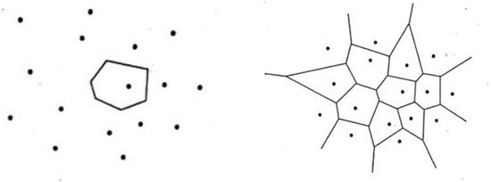
Figure 1.
Example of the Voronoi diagram.
The dual graph of is called the proximity graph or Delaunay graph of S and is denoted by . If the points are not aligned and there is no group of four cocircular vertices, the Delaunay graph is a triangulation. An example is shown in Figure 2.
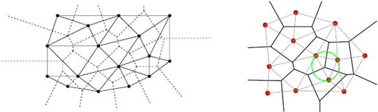
Figure 2.
Example of Delaunay graph.
Many researchers have studied the computation of Voronoi diagrams and Delaunay graphs; see, for example, [14,15,16,17,18].
We denote by the convex hull of a set , , that is, the boundary of the smallest convex polygon that encloses those points. Then we define an internal triangle as a triangle (3-cycle) whose three edges (but not necessarily its vertices) are located in the interior of the triangulation. Given a graph G, we will denote by the set of internal triangles of G.
3. Graph Theory and Sensor Networks
In this section, we explore the connection between graph theory and sensor networks. The main idea is to model a sensor network using a Delaunay graph, an approach that has been employed in previous studies [19,20,21].
Consider a group of sensors distributed across a planar field. Each sensor is represented as a vertex (or node) in the graph. These nodes serve as points for data collection and transmission, mirroring the physical location and function of the sensors within the network. The topology of the graph encapsulates the spatial distribution of sensors and their interconnections, providing an intuitive and visually meaningful representation of the network’s structure.
The edges of the graph represent the connections between the sensors in the network, encapsulating how these sensors communicate to exchange information. Specifically, the spatial arrangement of the sensors is used to construct the graph associated with the sensor network. Following this methodology, the Delaunay graph corresponding to the sensor network is formed by linking nodes that are sufficiently close to each other. Each sensor thus corresponds to a vertex in the Delaunay graph, and the physical proximity between sensors is depicted as edges within the graph. This approach ensures efficient connectivity, reflecting the geometric relationships between sensors in the network. We show an example of this association in Figure 3.
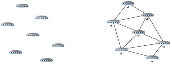
Figure 3.
Example of a group of sensors and its associated Delaunay graph.
In this paper, we deal with several graph tools such as vertex coloring and Eulerian and Hamiltonian paths. These tools and their connection with Delaunay graph have been studied previously in [22,23,24,25,26,27].
Now, in the next subsections, we propose several possible applications of these graph-theoretical tools to enhance the design and functionality of sensor networks. At the end of each of these subsections, we give an example concerning the Delaunay graph from Figure 3.
3.1. Eulerian Paths
Let us note that in a sensor network associated with a Delaunay graph, a Eulerian path represents a trail on the network that visits every communication link once. Studying this type of path can be useful to analyze network connectivity, optimize data transmission, avoid fault tolerance, and improve robustness.
First, computing Eulerian paths helps to find connectivity patterns among sensors and provides a systematic way to go through the whole network. The analysis of Eulerian path existence is crucial for identifying potential bottlenecks, ensuring uniform data distribution, and enhancing overall network resilience.
Next, this type of path contributes to optimizing the data transmission in a sensor network. By following these paths, data can be transmitted efficiently from one sensor to another, minimizing the risk of congestion. It can also help to reduce energy consumption.
Finally, Eulerian paths also play a very important role in enhancing the fault tolerance and robustness of a sensor network. By identifying alternative paths, the network can be adapted to changes such as sensor failures or environmental disruptions. This adaptability is essential for maintaining continuous data flow.
In order to show an example of this kind of trail, the Delaunay graph from Figure 3 is Eulerian. In fact, a Eulerian cycle is given by since it is a closed trail on the network visiting every communication link (edge) once.
3.2. Hamiltonian Paths
Computing Hamiltonian paths allows us to visit all sensors once, collecting all the data saved by them. Analyzing the existence of this type of trail can be applied to analyze network connectivity, optimize data collection, enhance routes efficiently, and improve network resilience.
In the field of sensor networks, the study of Hamiltonian paths within the Delaunay graph associated with such a network allows us to analyze the interconnectivity among sensors. These paths, covering every sensor node precisely once, provide optimal routes for traversing the sensor network.
Moreover, the analysis of this type of path contributes to the enhancement of routing efficiency; identifying paths that cover all sensors aids in designing communication routes that minimize delays and reduce the risk of congestion.
Finally, understanding Hamiltonian paths also plays a very important role in improving the resilience of a sensor network. By identifying paths that visit all the nodes, the network can adapt to changes, such as sensor failures, ensuring continuous data flow.
An example of a Hamiltonian cycle is given by the trail in the Delaunay graph from Figure 3 since it is a closed trail on the network visiting every node (vertex) once.
3.3. Vertex Coloring
Studying the chromatic number and vertex coloring of a Delaunay graph associated with a sensor network can be very interesting in order to distribute resources efficiently, avoid sensor interference, assign tasks or roles, identify conflicts, and improve route planning.
By assigning colors to the vertices of the graph, it is possible to find an optimal coloring which minimizes the total number of colors used. This can be applied to distribute resources efficiently, such as transmission frequencies or communication channels. It can also be applied to reduce energy consumption by activating or deactivating several sets of sensors.
Regarding interference management, vertex coloring helps to avoid interference between adjacent nodes that share communication channels.
In reference to task scheduling, this graph tool can be useful to assign specific tasks or roles to sensors based on their colors. This provides the implementation of scheduling and coordination strategies, allowing an efficient distribution of responsibilities within the sensor network.
Finally, vertex coloring can be very important in order to identify conflicts and avoid fault detection. This can be accomplished by planning new routes following some vertices that have the same color.
As an example, the chromatic number of the Delaunay graph from Figure 3 is 3. Moreover, a minimal vertex coloring for this graph is given as follows: the first color is for sensors , the second is for , and the third one is for .
4. Theoretical Results
In this section, we show several theoretical results regarding Eulerian or Hamiltonian paths and vertex coloring of Delaunay graphs.
4.1. Eulerian
First, it is possible to estimate the number of triangles for a Deluany graph according to its planarity and Euler’s Theorem as it is shown in the following.
Lemma 1.
The number of triangles in is at most .
Proof.
is planar; therefore, if is a graph with n vertices and m edges verifying . Moreover, according to Euler’s Theorem, , where is the number of faces of . That number of faces will be the number of triangles plus the external face. Therefore, . □
The number of triangles, and more concretely the internal ones, is related to the existence of Eulerian trails, as we show in the following.
Proposition 1.
If , then is not Eulerian. Furthermore, either or .
Proof.
Since , , that is, is not a 3-cycle. Now, we distinguish several cases.
Case 1:
Then, with , it is satisfied that . Indeed, if with verifies that , then is a 3-cycle. Furthermore, is an internal triangle since and , but this is a contradiction. Therefore, there exists a unique , has vertices, and .
Case 2:
Then, is the cycle where , adding some edges until creating the triangulation. This set of edges forms a connected graph and acyclic, that is, a tree T (otherwise, we would have vertices which are not in ). Therefore, . Since a tree has at least two leaves, such that and are leaves of T. Therefore, are vertices with degree three in and G is not Eulerian. □
4.2. Hamiltonian
The number of triangles, and more concretely the internal ones, is related to the existence of Hamiltonian cycles, as we show in the following results.
Proposition 2.
If , then is Hamiltonian. Furthermore, either or .
Proof.
First of all, we can assume that since in case that we would have a 3-cycle which is trivially Hamiltonian. Since , , that is, is not a 3-cycle. Now, we distinguish several cases.
Case 1:
Then, with , it is satisfied that . This is due to the fact that if with verifies that , then is a 3-cycle. Furthermore, is an internal triangle and , but this is a contradiction. Therefore, there exists a unique , has vertices, and . Therefore, is Hamiltonian since every wheel graph is.
Case 2:
Then, is the cycle , where n is the total number of vertices in V, adding some edges until creating the triangulation. Consequently, is Hamiltonian and the Hamiltonian cycle is given by . □
Proposition 3.
If , then is Hamiltonian.
Proof.
In the case that , we know that is Hamiltonian due to Proposition 2.
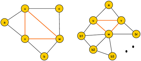
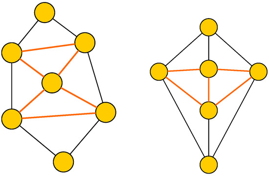
Let us assume that has one unique internal triangle, T, whose vertices are . Since T is an internal triangle, each one of the edges , , and belongs to another 3-cycle. Now, we have two possibilities. On one hand, we suppose that there exist another three vertices such that , , and determine the other three triangles containing the edges , , and , respectively. In this case, those vertices have degree two, and . Consequently, is the Hamiltonian cycle and we conclude that is Hamiltonian. On the other hand, if the previous situation is not satisfied, then , where a is the unique vertex with degree two. Moreover, a is adjacent to two vertices among . Without loss of generality, we can consider u and v to be those vertices. Then, w is the unique vertex which does not belong to and the graph induced by is a wheel graph defined by . Every wheel graph is Hamiltonian and that Hamiltonian cycle can be extended considering also the edges and . These two possible cases are represented in Figure 4.
Figure 4.
Delaunay graphs with one internal triangle.
Now, we suppose that has two internal triangles, and . We have two possible cases since these two triangles can share a vertex or an edge. In the case that and have a common vertex, u, they determine a friendship graph and the remaining vertices of belong to since otherwise there would be more than two internal triangles. Following a similar reasoning as before with the wheel graph, it is possible to obtain a Hamiltonian cycle containing the vertices from and u. In the case that and share an edge, then both triangles are contained in a 4-cycle, . The Hamiltonian cycle of is constructed by the union of and . We show an example of both situations in Figure 5. □
Figure 5.
Delaunay graphs with two internal triangles.
In [9], the authors proved that a Delaunay graph always contains a Hamiltonian path when the distance considered is the square one (-metric). It is an open problem if this is also true for the Euclidean distance. In the following proposition, we show that it is true that the previous statement is not true in case of Hamiltonian cycles.
Proposition 4.
There exist Delaunay graphs that are not Hamiltonian.
Proof.
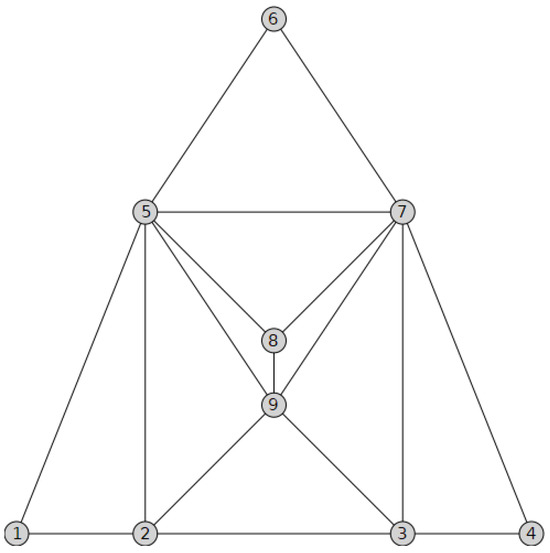
Let us consider the set of vertices and the Delaunay graph, , from Figure 6. Let C be a Hamiltonian cycle of . The neighbors of in C must be and , since they are the only adjacent vertices to . Similarly, the neighbors of have to be and and the neighbors of will be and . Every vertex on a cycle has exactly two adjacent vertices. Therefore, the neighbors of will be and and the neighbors of will be and . Consequently, and cannot be neighbors of in C. However, must have as neighbors two of the vertices . This is a contradiction. □
Figure 6.
Non-Hamiltonian Delaunay graph.
4.3. Vertex Coloring
In the following Lemma, we show the possible values for the chromatic number of a Delaunay graph.
Lemma 2.
Let G be a Delaunay graph. Then, equals 3 or 4.
Proof.
First, G is formed by triangles and the chromatic number of this type of graphs is three. Therefore it is obvious that . Moreover, G is a planar graph and, according to the well-known four-color theorem, it is satisfied that . Consequently, . □
Next, we give several results concerning sufficient conditions under which the chromatic number is three.
Proposition 5.
Let G be a Delaunay graph. If G is Eulerian, then .
Proof.
Let G be a Delaunay Eulerian graph. According to Euler’s Theorem, all the vertices of G have even degree. Let us denote by V the set of vertices of G. Then, V can be decomposed as , where is the set of vertices of degree two and is the set of vertices with even degree greater or equal to four. Now, we show how to develop the vertex coloring of all the vertices in . Notice that the vertices in this set are common vertices of at least three triangles. In this way, we start choosing one of these vertices and go through all its adjacent triangles, coloring the vertices alternatively and keeping the condition that there are no adjacent vertices with the same color. This is possible due to the fact that all the vertices have even degrees. In the case that there is a vertex with odd degree, we will not succeed in this procedure with only three colors. After this, we continue coloring the vertices from the set . Let us note that there are no pairs of vertices with degree two that are mutually adjacent, since in that case G would contain an internal face which is not a triangle. Due to this, every vertex in is adjacent to an internal triangle and can be colored according to the two colors already chosen for the other two vertices adjacent to x. □
Proposition 6.
Let G be a Delaunay graph, which does not contain with n being even as a subgraph. Then, .
Proof.
First, notice that G is a planar graph formed by triangles. Therefore, if G does not contain any wheel graphs with an even number of vertices as a subgraph, then G will not have any subgraphs with a chromatic number equaling four. This is due to the fact that the graphs made up of triangles whose chromatic number is equal to four contain as a subgraph the complete graph , which is isomorphic to , or a wheel graph with an even number of vertices.
In order to obtain the 3-coloring of G, it suffices to follow the method explained in Proposition 5. □
Corollary 1.
If all the vertices of a Delaunay graph, G, belong to , then .
Proof.
Let be a Delaunay graph such that . Then, G does not contain as a subgraph . It follows from Proposition 6 that . □
Corollary 2.
If a Delaunay graph, G, verifies that , then .
Proof.
It follows from Corollary 1 and the fact that if G has no internal triangles, then all the vertices of G belong to . □
Remark 1.
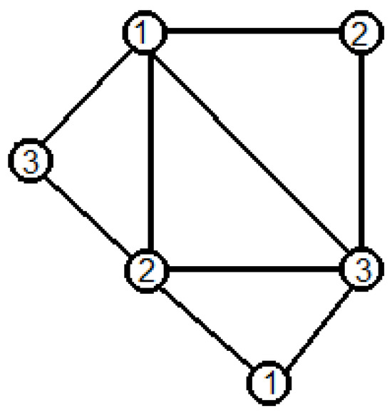
Obviously the reciprocal of the previous corollary is not true. Moreover, the condition of having no internal triangles is not equivalent to the fact that all the vertices of G belong to the convex hull of G. For example, the Delaunay graph of Figure 7 has one internal triangle and it is possible to obtain a 3-vertex coloring as indicated in that same figure.
Figure 7.
Delaunay graph with one internal triangle.
5. Algorithmic Procedures
In this section, we show several new algorithms concerning the existence of Eulerian or Hamiltonian trails and the vertex coloring of a Delaunay graph. We have not found in the literature any of these algorithms for those kinds of graphs.
These algorithmic procedures have been implemented by using the symbolic computation package Maple, working with the implementation in version 22. Maple employs a proprietary programming language tailored for symbolic computation, mathematical modeling, and problem-solving. It supports procedural and functional programming paradigms, enabling the use of loops, conditionals, and custom functions while excelling in symbolic manipulation of equations and algebraic structures. The language also facilitates efficient matrix operations and numerical calculations, making it suitable for diverse mathematical applications. Its syntax, although unique, is intuitive for users familiar with mathematical programming, providing functionality similar to Python or MATLAB but specifically optimized for symbolic and algebraic computations.
In order to carry out the implementation, the libraries GraphTheory, RandomGraphs, geometry, ListTools, ComputationalGeometry, and GeometricGraphs have to be used in order to activate commands related to graphs, lists, and computational geometry. Before running the procedures, we need the command restart to reset all the variables and delete all the computations saved in the kernel.
5.1. Eulerian
This algorithmic procedure allows us to determine whether a graph is Eulerian. Additionally, it identifies the Eulerian cycle or path if the graph is semi-Eulerian. We implement the procedure eulerianGraph, which takes a graph G as input. The output is either the Eulerian cycle (if the graph is Eulerian), the semi-Eulerian path (if the graph is semi-Eulerian), or a message indicating that the graph does not meet the necessary conditions.
The implementation begins by verifying if the graph is Eulerian using the function . If the graph is Eulerian, a message is displayed along with the trail T, which represents the Eulerian cycle. If the graph is not Eulerian, we calculate the number of vertices with an odd degree, noting that a graph is semi-Eulerian if it has exactly two vertices with odd degrees. In such cases, we apply a depth-first search (DFS) algorithm to traverse the graph, construct a path that visits all vertices and edges, and output the semi-Eulerian path. If none of these conditions are satisfied, the procedure outputs a message stating that the graph is neither Eulerian nor semi-Eulerian.
- > eulerianGraph := proc(H)> local count, i, j, v, w, path, verts, N, vertices, edges, visited;> if IsEulerian(H, ’T’) then> print("The graph is eulerian’’);> print(The eulerian cycle is T);> else> count := 0;> verts := [];> for v in Vertices(H) do> if type(Degree(H, v), odd) then> count := count + 1;> verts := [op(verts), v];> fi; od;> if count = 2 then> print(‘‘The graph is semieulerian’’);> vertices := Vertices(H);> edges := Edges(H);> visited := {op(vertices)};> path := [];> for i to nops(edges) do> if edges[i][1] = verts[1] and not edges[i] in visited then> visited := visited union {edges[i]};> path := [op(path), verts[1], edges[i][2]];> w := edges[i][2];> break;> elif edges[i][2] = verts[1] and not edges[i] in visited then> visited := visited union {edges[i]};> path := [op(path), verts[1], edges[i][1]];> w := edges[i][1];> break;> fi; od;> while nops(path) <= nops(edges) do> N := Neighbors(H, w);> for i to nops(N) do> for j to nops(edges) do> if edges[j][1] = w and edges[j][2] = N[i] and not edges[j] in visited then> visited := visited union {edges[j]};> path := [op(path), N[i]];> w := N[i];> break;> elif edges[j][2] = w and edges[j][1] = N[i] and not edges[j] in visited then> visited := visited union {edges[j]};> path := [op(path), N[i]];> w := N[i];> break;> fi; od; od; od;> print(‘‘Semieulerian Path:’’, path);> else> print(‘‘The graph isn’t eulerian or semieulerian’’);> fi; fi;> end proc:
Now, we implement another algorithmic procedure, which studies if a graph is Eulerian or not based on Lemma 1. We have implemented four subroutines: createHullEdges, findOtherEdges, countElements, and isK3.
The first subprocedure, called createHullEdges, receives as input the convex hull of the graph, . The output is a list of the edges that belong to the convex hull. Concerning the implementation, it takes the list of vertices of the convex hull and create a list of the edges that join them.
- > createHullEdges := proc(hull)> local edges, i;> edges := [];> for i to nops(hull) - 1 do> edges := [op(edges), {hull[i + 1], hull[i]}];> od;> edges := [op(edges), {hull[-1], hull[1]}];> return edges;> end proc:
The next subroutine is called findOtherEdges. It receives as input the list of edges of the graph and the edges that belong to the convex hull, which is the output of createHulledges. The output is the list of edges that do not belong to the convex hull. Concerning the implementation, it analizes if every edge is in the list of the edges that belong to the convex hull, and, if it is not there, it is added to a new list: .
- > findOtherEdges := proc(allEdges, hullEdges)> local otherEdges, edge, i;> otherEdges := [];> for edge in allEdges do> if not edge in hullEdges then> otherEdges := [op(otherEdges), edge];> fi; od;> return otherEdges;> end proc:
Now, we show the implementation of the subroutine countElements, which receives as input the list . The output is a list with the number of the times that each vertex is repeated in . Regarding the implementation, it starts iterating through each pair in and appends its elements to . Then, it iterates over this new list and counts its occurrences. If the element is already in the list, it finds its index and adds one to the count. Otherwise, the count is set to 1. Finally, combines the unique elements from and their counts into pairs.
- > countElements := proc(otherEdges)local elements, counts, element, i, vertexSet, pair, Index, elementCounts;> vertexSet := [];> for pair in myList do> vertexSet := [op(vertexSet), op(pair)];> od;> elements := [];> counts := [];> for element in vertexSet do> if element in elements then> Index := NULL;> for i to nops(elements) do> if elements[i] = element then> Index := i;> break;> fi; od;> counts[Index] := counts[Index] + 1;> else elements := [op(elements), element];> counts := [op(counts), 1];> fi; od;> elementCounts := [seq([elements[i], counts[i]], i = 1 .. nops(elements))];> return elementCounts;> end proc:
Finally, we develop the implementation of the procedure isK3. It receives as input . The output is a string which says that the graph is Eulerian and how many internal triangles it has or that it is not Eulerian. For the implementation, the routine considers and uses countElements. We obtain the list and check if every vertex is repeated twice. In that case, the graph is Eulerian and it has only one internal triangle. Otherwise, the procedure checks if the number of vertices that are not repeated twice is multiple of 2. If so, the graph is Eulerian and it has internal triangles. Any other case means that the graph is not Eulerian.
- > isK3 := proc(otherEdges)> local vertices, vertexSet, i, j, pair, count, counts, index, G;> counts := countElements(otherEdges);> count := 0;> index := [];> for i to nops(counts) do> if counts[i][2] = 2 then> count := count + 1;> else> index := [op(index), i];> fi; od;> if count = nops(counts) then> return ‘‘Yes, there is 1 intern K3’’;> else> count := 0;> for i in index do> if counts[i][2] mod 2 = 0 then> count := count + 1;> fi; od;> if count = nops(index) then> return ‘‘Yes, all the intern edges create ’’, 1/3*nops(otherEdges), ‘‘ K3’’;> else> return ‘‘No, all the intern edges do not create K3’’;> fi; fi;> end proc:
5.2. Hamiltonian
We can determine whether a graph is Hamiltonian using the following algorithmic procedure. Additionally, this approach identifies the Hamiltonian cycle or path if the graph is semi-Hamiltonian. The implemented procedure, hamiltonianGraph, takes a graph H as its input. The output is the Hamiltonian cycle (if the graph is Hamiltonian), the semi-Hamiltonian path (if the graph is semi-Hamiltonian), or a message indicating that the graph does not satisfy the required conditions.
Regarding the implementation, it first verifies if the graph is Hamiltonian, using the function . In such a case, it prints a message and the trail T, which is the Hamiltonian cycle. In the case that the graph is not Hamiltonian, the procedure tries to find the path starting from the first vertex. In that process, it looks at the neighbors of the vertex and sees if they have been visited or if they are articulation points. If both conditions are not fulfilled, it adds the first neighbor in the path and repeats the process based on it. In the case that the vertex is an articulation point, it is only added if it is the only one that has not been visited. The procedure only stops when there are not new vertices to add to the path. Then, it tries the same process starting with the next vertex of the graph.
If, after repeating the process starting with each vertex, the procedure can not find a path as long as the number of vertices, the procedure prints a message indicating that the graph is not Hamiltonian or semi-Hamiltonian.
- > hamiltonianGraph := proc(H)> local count, vertices, v, v1, w, i, j, path, N, artP, indexap, indexnp;> if IsHamiltonian(H, ’C’) then> print(The graph is Hamiltonian);> print(The Hamiltonian cycle is C);> else> vertices := Vertices(H);> artP := ArticulationPoints(H);> for v in vertices do> path := [v];> w := v;> while nops(path) < nops(vertices) do> N := Neighbors(H, w);> indexap := [];> indexnp := [];> for i from 1 to nops(N) do> if N[i] in artP then> indexap := [op(indexap), i];> fi;> if not N[i] in path then> indexnp := [op(indexnp), i];> fi; od;> if nops(indexnp) = 0 then> break;> fi;> if nops(indexnp) = 1 and indexnp = indexap then> path := [op(path), N[op(indexap)]];> w := N[op(indexap)];> fi;> for i from 1 to nops(N) do> if not N[i] in path and not i in indexap then> path := [op(path), N[i]];> w := N[i];> break;> fi; od; od;> if nops(path) = nops(vertices) then> print(‘‘The graph is semihamiltonian’’);> print(‘‘Semihamiltonian Path:’’, path);> break;> fi; od; fi;> if nops(path) <> nops(vertices) then> print(‘‘The graph isn’t hamiltonian or semihamiltonian’’);> fi;> end proc:
In the next algorithm, called hamiltonianGraph, we have added the Rahman–Kaykobad Theorem (see [28]):
Theorem 1.
Let be a connected graph with n vertices such that for all pairs of distinct nonadjacent vertices one has . Then, G has a Hamiltonian path.
This implies that the semi-Hamiltonian path is not going to be calculated unless the condition is fulfilled.
- > hamiltonianGraph := proc(H)> local count, verts, vertices, v, v1, w, i, j, path, N, artP, indexap,> indexnp, cond, countcond;> if IsHamiltonian(H, ’C’) then> print(The graph is Hamiltonian);> print(The Hamiltonian cycle is C);> else> vertices := Vertices(H);> count := 0;> countcond := 0;> artP := ArticulationPoints(H);> for v in vertices do> verts := [];> N := Neighbors(H, v);> for v1 in vertices do> if not v1 in N and v1 <> v then> verts := [op(verts), v1];> fi; od;> for i from 1 to nops(verts) do> for j from i + 1 to nops(verts) do> cond := Degree(H, verts[i]) + Degree(H, verts[j]) +> nops(ShortestPath(G, verts[i], verts[j]));> count := count + 1;> if nops(vertices) < cond then> countcond := countcond + 1;> fi; od; od; od;> if count = countcond then> print(‘‘The graph is semihamiltonian’’);> for v in vertices do> path := [v];> w := v;> while nops(path) < nops(vertices) do> N := Neighbors(H, w);> indexap := [];> indexnp := [];> for i from 1 to nops(N) do> if N[i] in artP then> indexap := [op(indexap), i];> fi;> if not N[i] in path then> indexnp := [op(indexnp), i];> fi; od;> if nops(indexnp) = 0 then;> break;> fi;> if nops(indexnp) = 1 and indexnp = indexap then> path := [op(path), N[op(indexap)]];> w := N[op(indexap)];> fi;> for i from 1 to nops(N) do> if not N[i] in path and not i in indexap then> path := [op(path), N[i]];> w := N[i];> break;> fi; od; od;> if nops(path) = nops(vertices) then> print(‘‘Semihamiltonian Path:’’, path);> break;> fi; od;> else> print(‘‘The graph isn’t hamiltonian or semihamiltonian’’);> fi; fi;> end proc:
5.3. Vertex Coloring
The following algorithmic procedures explore the potential relationship between a graph being Eulerian or containing a wheel graph as a subgraph and its chromatic number. This process comprises two subroutines: wheelCondition and chromaticNum. In the first subroutine, wheelCondition, the algorithm examines a given graph to determine whether it contains any subgraphs or if the graph itself is a wheel graph. This is achieved using the function . It is known that if a graph is, or contains, a wheel graph with an even number of vertices, its chromatic number must be 4. Therefore, the implementation begins by searching for even wheel graphs. If no even wheel graphs are found, the algorithm searches for odd wheel graphs, which indicate a chromatic number of 3. If no wheel subgraph is detected, the procedure outputs a message stating this result.
- > wheelCondition := proc(H)> local n, Wn, isomorphicResult;> for n from 3 by 2 to 19 do> Wn := WheelGraph(n);> isomorphicResult := IsSubgraphIsomorphic(Wn, H, isomorphism);> if not (isomorphicResult = false) then> print(‘‘The graph or a subgraph is a Wheel Graph’’, W_{n + 1});> print(‘‘The wheel graph is even’’);> print(‘‘The chromatic number must be 4’’);> break;> fi; od;> if isomorphicResult = false then> for n from 4 by 2 to 20 do> Wn := WheelGraph(n);> isomorphicResult := IsSubgraphIsomorphic(Wn, H, isomorphism);> if not (isomorphicResult = false) then> print(‘‘The graph or a subgraph is a Wheel Graph’’, W_{n + 1});> print(‘‘The wheel graph is odd’’);> print(‘‘The chromatic number must be 3’’);> break;> fi;> if n = 20 then> print(‘‘The graph or a subgraph is not a Wheel Graph’’);> fi; od; fi;> end proc:
With the second subroutine, chromaticNum, we validate the results obtained. First, we see if the graph is Eulerian, in which case, the chromatic number is 3. If the graph is not Eulerian, we use the first subroutine, wheelCondition, to study the subgraphs. Then, we use the Maple function to find the chromatic number and see if it matches with the result obtained.
- > chromaticNum := proc(H)> if IsEulerian(H, ’T’) then> print(‘‘The graph is Eulerian’’);> print(‘‘The chromatic number must be 3’’);> else> print(‘‘The graph is not Eulerian’’);> WheelCondition(H);> fi;> print(‘‘The chromatic number is:’’, ChromaticNumber(H, ’col’));> print(col);> end proc:
6. Case Study: Monitorization of a Sugar Cane Field
All the algorithms proposed in the previous section can be used to manage the devices in an agricultural field. This is the case of the situation presented here, in which we show two examples for the monitorization of two soil variables—moisture and temperature—of a sugarcane field that were needed to control the irrigation. The monitorization network is built with a set of devices, called nodes, which have different capabilities: measurement of soil moisture and temperature; computation, to execute some local filters and routines, and storing; and communication of the processed data using the LoRaWAN protocol. The heart of each node is a Lopy4 board from Pycom, whose core is an ESP32 processor. A photograph of the node is shown in Figure 8.
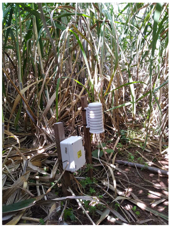
Figure 8.
Deployed node in a sugarcane field.
In the first example, a set of 12 nodes was deployed in a meters field close to the city of Arroyos y Esteros in Paraguay (Longitude West; Latitude South). The location of the nodes is depicted in Figure 9, where the x-axis is aligned with the direction of the sugarcane planks.
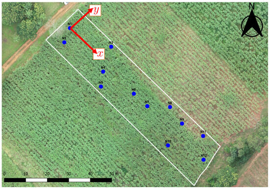
Figure 9.
Aerial photography of the sugarcane field with the nodes marked with blue dots.
Now, we consider the 12 nodes from Figure 9 and define the variable PTS containing the Euclidean coordinates of each node.
- PTS:=[[5,13],[10,6],[25,28],[30,20],[35,3],[45,11],[55,16],[60,29],[75,22],[80,5],[85,28],[95,12]];
In Figure 10, we show the Voronoi diagram and weighted Delaunay graph associated with the nodes.
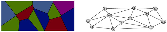
Figure 10.
Voronoi diagram and weighted Delaunay graph associated with the sugarcane field.
Now, we are going to apply the different algorithms in the Delaunay graph created from the sugarcane field.
First, when we run the routine eulerianGraph, we obtain the output
This is due to the fact that our Delaunay graph contains more than two vertices with odd degrees. If we apply the algorithmic procedures based on the Lemma 1, createHullEdges, findOtherEdges, countElements, and isK3, we obtain:
As a consequence of this, it is not possible to design a trail in the sensor network that visits every communication link once.
Next, we execute the routine called hamiltonianGraph obtaining:
Consequently, it is possible to visit all sensors once following a closed trail in order to collect all the data saved by them. The sequence obtained gives us the node order that should be followed.
Finally, we analyze some properties of our sensor network related to the chromatic number using wheelCondition and chromaticNum. The outputs obtained are as follows:
In this way, the chromatic number of our Delaunay graph associated with the sugar cane field is 4 and we also know the color of each vertex. This allows us to assign different tasks or roles to adjacent nodes in a minimal way. The first task would be assigned to nodes , and 12. Then, the second one would be assigned to vertices and 9, the third one to and 10, and the last one to nodes 4 and 11. Another possible application is to avoid interference between adjacent vertices by developing the previous assignment considering channels instead of tasks. In case of energy consumption issues, we can activate the group of sensors associated with one color and deactivate the other ones. It could be an efficient way of saving energy since the communication links are not working since there is no pair of adjacent nodes activated.
Now, we show a second example by considering eight sensors in the sugarcane field that define the variable as follows:
- PTS := [[9, 43], [12, 3], [20, 30], [29, 18], [49, 5], [57, 38], [76, 52], [90, 39]]
In Figure 11, we show the Voronoi diagram and weighted Delaunay graph associated with these nodes.
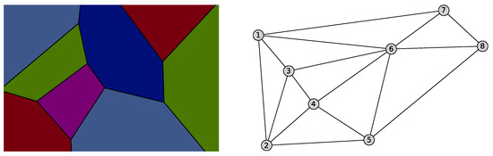
Figure 11.
Voronoi diagram and weighted Delaunay graph associated with the second example.
Now, we run the routine eulerianGraph and obtain the output
This means that our Delaunay graph has only two vertices with odd degrees. If we apply the algorithmic procedures based on Lemma 1, createHullEdges, findOtherEdges, countElements, and isK3, we obtain:
Figure 12 shows the internal triangles.
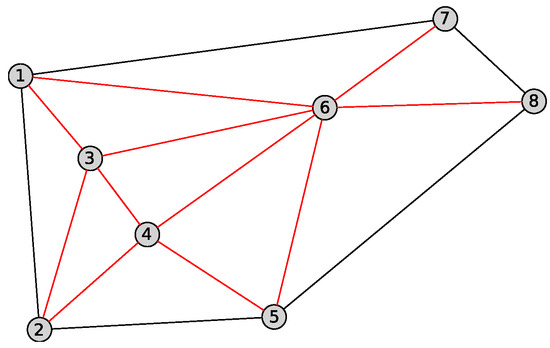
Figure 12.
Internal triangles create K3.
Next, we execute the algorithm hamiltonianGraph and we obtain:
The result is the order we should follow to visit every sensor once in a closed trail.
Finally, we evaluate the two subroutines wheelCondition and chromaticNum. The outputs obtained are:
Consequently, the chromatic number of the Delaunay graph considered in this second example is 3 and we also know the color of each vertex. This allows us to minimize the tasks or roles assigned to the nodes. The first one would be assigned to nodes 2 and 6, the second one to vertices , and 8, and the last one to , and 7. It is also possible to avoid interference or save energy considering the previous assignment as we mentioned for the first example.
7. Computational and Complexity Study
Now, a computational study and statistics related to the algorithmic procedures in Section 5 are shown. The algorithms have been implemented with MAPLE 22 with an Intel Core i5-1038NG7 with a 2.0 GHz processor and 16.00 GB of RAM. Table 1, Table 2, Table 3 and Table 4 show some computational data about both the computing time and the memory used to return the output of the procedures eulerianGraph, hamiltonianGraph, hamiltonianGraph2, and chromaticNum, respectively, according to the number of sensors.

Table 1.
Computing time and used memory for eulerianGraph.
Table 2.
Computing time and used memory for hamiltonianGraph.
Table 3.
Computing time and used memory for hamiltonianGraph2.
Table 4.
Computing time and used memory for chromaticNum.
Next, we show some brief statistics about the relation between the computing time and the memory used by the implementation of the previous algorithms. Figure 13 and Figure 14 show, respectively, the behavior of the computing time (C.T.) and used memory (U.M.) with respect to the number of sensors, n, for every algorithm. We can see how the computational time increases more slowly for routine eulerianGraph than the other three. Moreover, that increment is greater for procedures hamiltonianGraph and hamiltonianGraph2 than the others. It seems that the computing time fits an exponential model for the two algorithm previously mentioned and this is not true for the remaining ones. Concerning the computing time, it does not seem to follow an exponential model since the growth is quite smooth. Figure 15 represents a frequency diagram for the quotient between used memory and computing time. In this case, the behavior for algorithm hamiltonianGraph2 seems to fit a negative exponential model, but this is not true for the remaining routines.
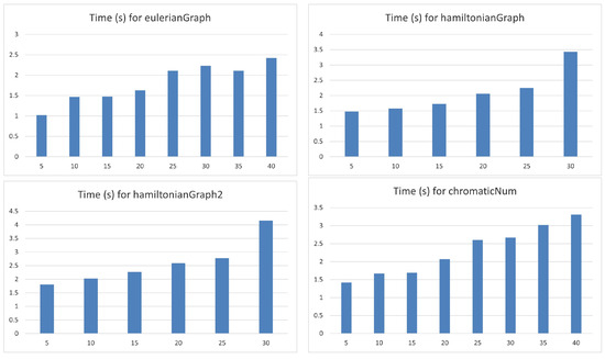
Figure 13.
Graphs for the C.T. with respect to the number of sensors.
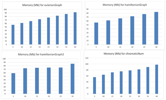
Figure 14.
Graphs for the U.M. with respect to the number of sensors.
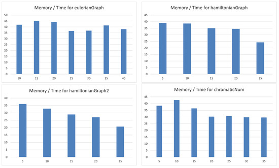
Figure 15.
Graphs for quotients U.M./C.T. with respect to the number of sensors.
Finally, the complexity of the algorithm is computed considering the number of operations carried out in the worst case. In order to express the complexity, the big O notation is used (see [29]): given , , .
Let us denote by the number of operations for the procedure i. This function depends on the number of sensors n. Table 5 shows the number of operations and the complexity of each routine.
Table 5.
Complexity and number of operations.
8. Discussion
In this paper, we have dealt with several algorithmic procedure regarding the existence of Eulerian or Hamiltonian trails and the vertex coloring of a Delaunay graph. Although we have not found any algorithms for this kind of graph in the literature, it is true that there are several algorithmic routines for these tools in the case of a general graph G.
First, Fleury’s and Hierholzer’s algorithms are classic approaches for finding Eulerian paths and cycles in graphs. Fleury’s algorithm, developed in the 19th century, is straightforward and relies on carefully selecting edges to avoid breaking the graph into disconnected components unless no alternative exists. This method has a time complexity of , where e is the number of edges in the graph. This means that Fleury’s algorithm can reach complexity of in the case of a dense graph with n vertices. In Table 5, we show that the complexity order of our routine eulerianGraph is in the worst case. This means that our algorithm has a lower complexity order than Fleury’s. However, this is not true for Hierholzer’s algorithm, whose complexity order is , i.e., in the worst case.
Our algorithm hamiltonianGraph in our study efficiently checks for Hamiltonian cycles and semi-Hamiltonian paths, with a complexity of for dense graphs due to the need to explore all vertices, articulation points, and neighbors. This is notably more efficient than classical backtracking algorithms (whose complexity order is ) and dynamic programming approaches (where its complexity order is . Our algorithm also benefits from graph-specific optimizations (e.g., Rahman–Kaykobad’s theorem and articulation point analysis), making it highly suitable for Delaunay graphs in sensor networks. This geometric focus allows it to outperform general algorithms in sparse graphs but may struggle with dense graphs, where the number of edges grows quadratically with the number of vertices, n, leading to increased memory usage. Therefore, future improvements could focus on optimizing its performance in denser graphs.
The algorithms in our study for computing the chromatic number in Delaunay graphs use two subroutines: wheelCondition and chromaticNum. The wheelCondition subroutine checks for isomorphism with wheel graphs to determine whether the chromatic number is 3 or 4. If the graph is not Eulerian, the chromaticNum procedure calls wheelCondition and computes the chromatic number using Maple’s ChromaticNumber function, which has a complexity of . When compared to other algorithms, greedy algorithms (which have a complexity of are faster but may not always provide the optimal solution, while backtracking methods, which have a complexity of , are less efficient for large graphs. Our approach is efficient for sparse graphs due to the use of specific graph properties but may become less efficient with dense graphs. Furthermore, heuristic methods like genetic algorithms offer faster approximate solutions but may not guarantee accuracy. Thus, our algorithms are well suited for smaller or sparse graphs but may need optimization for larger or denser networks.
In short, our algorithms provide an efficient solution for Delaunay graphs in sensor networks, balancing complexity and accuracy. While they excel in leveraging graph-specific properties, they may struggle with dense graphs. Future work could expand their applicability and explore parallelization for better performance on large datasets.
9. Conclusions
In this paper, we have explored the intersection between graph theory and sensor networks, highlighting the analytical and visually intuitive framework that this synergy provides. By leveraging graph-based approaches, we can simplify the representation of the complex structures inherent to sensor networks, facilitating informed decision-making for their optimization, maintenance, and evolution. This connection between the two disciplines offers promising advancements in intelligent data management and improved operational efficiency across various applications.
The study of vertex coloring and Eulerian and Hamiltonian characteristics has proven particularly valuable in analyzing network connectivity, optimizing data transmission, mitigating failures or interference, and enhancing network resilience. These tools not only improve the overall robustness of sensor networks but also support their scalability and adaptability to ever-changing conditions.
From the authors’ perspective, the algorithms, tools, and results presented in this work provide a solid foundation for understanding and advancing the relationship between graph theory and sensor networks. We aim to continue developing this research line in the future to uncover new insights and applications.
Moreover, the methodologies discussed in this paper extend beyond sensor networks. For example, geographic information systems (GISs) can utilize Eulerian and Hamiltonian paths in Delaunay graphs to optimize navigation and routing within geographic networks such as road systems or natural landscapes. These techniques are particularly relevant in fields like environmental monitoring, disaster response, and urban planning, where efficient traversal and pathfinding are critical.
Similarly, wireless communications and 5G network design present another promising application. Delaunay graphs, often used to model interference-limited regions, benefit from vertex coloring algorithms for efficient frequency allocation and interference minimization. Additionally, Hamiltonian paths offer potential improvements in network resilience by identifying optimal data transmission routes, ensuring robustness against node failures, and enhancing overall reliability and efficiency.
Author Contributions
All authors have worked equally in every aspect: conceptualization, methodology, software, validation, formal analysis, investigation, preparation, funding acquisition, project administration, and writing. All authors have read and agreed to the published version of the manuscript.
Funding
This research was funded by the Ministry of Science and Innovation with grant number PID2020-117800GB-I00.
Data Availability Statement
The authors declare that there are no data associated with this work.
Acknowledgments
This work has been partially supported by FQM-326 and PID2020-117800GB-I00.
Conflicts of Interest
The authors declare no conflicts of interest.
References
- Ameen, A.; Ali, A.; Khattab, M.; Aliesawi, S. Employing Graph Theory in Enhancing Power Energy of Wireless Sensor Networks. J. Inf. Sci. Eng. 2020, 36, 323–335. [Google Scholar]
- Charalampopoulos, P.; Pitoura, E. Graph-based algorithms for wireless sensor networks. In Foundations and Applications of Sensor Management; Springer: Berlin, Germany, 2012; pp. 125–146. [Google Scholar]
- Bomgni, A.B.; Mdemaya, G.B.J.; Sindjoung, M.L.F.; Velempini, M.; Djoko, C.C.T.; Myoupo, J.F. CIBORG: CIrcuit-Based and ORiented Graph theory permutation routing protocol for single-hop IoT networks. J. Netw. Comput. Appl. 2024, 231, 103986. [Google Scholar] [CrossRef]
- Hegde, R.; Sudha, P.; Bhat, M. A Graph Theory Approach to Load Balancing in Wireless Sensor Network. 2019. Available online: https://www.researchgate.net/publication/338118140_A_Graph_Theory_Approach_to_Load_Balancing_in_Wireless_Sensor_Network#fullTextFileContent (accessed on 1 September 2024).
- Misra, S.; Reisslein, M. Graph-theoretic analysis of connectivity in wireless sensor networks. IEEE Trans. Wirel. Commun. 2009, 8, 966–975. [Google Scholar]
- Bayón-Gutiérrez, M.; Alaiz-Moretón, H.; García-Rodríguez, I.; Benavides, C.; García-Ordás, M.T.; Benítez-Andrades, J.A. Minimum cost Eulerian cycles in road networks. In Proceedings of the 17th Iberian Conference on Information Systems and Technologies (CISTI), Madrid, Spain, 22–25 June 2022; pp. 1–6. [Google Scholar] [CrossRef]
- Li, H.; Liu, Q.; Ma, X.; Qi, Q.; Liu, J.; Zhao, P.; Yang, Y.; Zhang, X. Cooperative Recharge Scheme Based on a Hamiltonian Path in Mobile Wireless Rechargeable Sensor Networks. Math. Probl. Eng. 2022, 2022, 6955713. [Google Scholar] [CrossRef]
- Rizzo, L.M.; Urrutia, S.; Loureiro, A.A.F. Role Assignment in Wireless Sensor Networks Based on Vertex Coloring. In Proceedings of the 2013 IEEE Seventh International Symposium on Service-Oriented System Engineering, San Francisco, CA, USA, 25–28 March 2013; pp. 537–545. [Google Scholar] [CrossRef]
- Ábrego, B.M.; Arkin, E.M.; Fernández-Merchant, S.; Hurtado, F.; Kano, M.; Mitchell, J.S.B.; Urrutia, J. Matching points with squares. Discret. Comput. Geom. 2009, 41, 77–95. [Google Scholar] [CrossRef][Green Version]
- Bollobás, B. Modern Graph Theory; Springer: Berlin, Germany, 1998. [Google Scholar]
- Aurenhammer, F.; Klein, R.; Lee, D. Voronoi Diagrams And Delaunay Triangulations; World Scientific Publishing Company: Hackensack, NJ, USA, 2013; pp. 1–348. [Google Scholar]
- Euler, L. Solutio problematis ad geometriam situs pertinentis. Comment. Acad. Sci. Petropolitanae 1736, 8, 128–140. [Google Scholar]
- Hamilton, W.R. Account of the Icosian Calculus. Proc. R. Ir. Acad. 1858, 6, 415–416. [Google Scholar]
- Cheng, S.W.; Dey, T.K.; Shewchuk, J.R. Delaunay Mesh Generation; CRC Press: Boca Raton, FL, USA, 2012. [Google Scholar]
- Chen, R.; Gotsman, C. Localizing the Delaunay triangulation and its parallel implementation. In Transactions on Computational Science XX; Gavrilova, M.L., Tan, C., Kalantari, B., Eds.; Volume 8110 of Lecture Notes in Computer Science; Springer: Berlin/Heidelberg, Germany, 2013; pp. 39–55, Extended abstract in ISVD 2012, pp. 24–31. [Google Scholar]
- Guibas, L.J.; Stolfi, J. Primitives for the manipulation of general subdivisions and the computation of Voronoi diagrams. ACM Trans. Graph. 1985, 4, 74–123. [Google Scholar] [CrossRef]
- Okabe, A.; Boots, B.; Sugihara, K.; Chiu, S.N. Spatial Tessellations: Concepts and Applications of Voronoi Diagrams, 2nd ed.; Wiley Series in Probability and Statistics; John Wiley and Sons Ltd.: Chichester, UK, 2000; with a foreword by D. G. Kendall. [Google Scholar]
- Reem, D. The projector algorithm: A simple parallel algorithm for computing Voronoi diagrams and Delaunay graphs. Theoret. Comput. Sci. 2023, 970, 114054. [Google Scholar] [CrossRef]
- Ghosh, P.; Gao, J.; Gasparri, A.; Krishnamachari, B. Distributed hole detection algorithms for wireless sensor networks. In Proceedings of the 2014 IEEE 11th International Conference on Mobile Ad Hoc and Sensor Systems, Philadelphia, PA, USA, 28–30 October 2014; pp. 257–261. [Google Scholar]
- Shao, C. Wireless sensor network target localization algorithm based on two- and three-dimensional Delaunay partitions. J. Sens. 2021, 2021, 4047684. [Google Scholar] [CrossRef]
- Wang, Y.; Li, X.-Y. Efficient Delaunay-based localized routing for wireless sensor networks: Research articles. Int. J. Commun. Syst. 2007, 20, 767–789. [Google Scholar] [CrossRef]
- Ackerman, E.; Keszegh, B.; Pálvölgyi, D. Coloring Delaunay-edges and their generalizations. Comput. Geom. 2021, 96, 101745. [Google Scholar] [CrossRef]
- Bonichon, N.; Gavoille, C.; Hanusse, N.; Ilcinkas, D. Connections between thetagraphs, Delaunay triangulations, and orthogonal surfaces. In Graph Theoretic Concepts in Computer Science; Thilikos, D.M., Ed.; Springer: Berlin/Heidelberg, Germany, 2010; pp. 266–278. [Google Scholar]
- Bose, P.; Cano, P.; Saumell, M.; Silveira, R.I. Hamiltonicity for convex shape Delaunay and Gabriel graphs. Comput. Geom. 2020, 89, 101629. [Google Scholar] [CrossRef]
- Bose, P.; Carmi, P.; Collette, S.; Smid, M. On the stretch factor of convex Delaunay graphs. J. Comput. Geom. 2010, 1, 41–56. [Google Scholar]
- Crapo, H.; Laumond, J.-P. Hamiltonian cycles in Delaunay complexes. In Geometry and Robotics; Boissonnat, J.D., Laumond, J.P., Eds.; Springer: Berlin/Heidelberg, Germany, 1989; pp. 292–305. [Google Scholar]
- Tomon, I. Coloring lines and Delaunay graphs with respect to boxes. Random Struct. Algorithms 2024, 64, 645–662. [Google Scholar] [CrossRef]
- Sohel-Rahman, M. and Kaykobad, M. On Hamiltonian cycles and Hamiltonian paths. Inf. Process. Lett. 2005, 94, 37–41. [Google Scholar] [CrossRef]
- Wilf, H.S. Algorithms and Complexity; Prentice Hall: Englewood Cliffs, NJ, USA, 1986. [Google Scholar]


Disclaimer/Publisher’s Note: The statements, opinions and data contained in all publications are solely those of the individual author(s) and contributor(s) and not of MDPI and/or the editor(s). MDPI and/or the editor(s) disclaim responsibility for any injury to people or property resulting from any ideas, methods, instructions or products referred to in the content. |
© 2024 by the authors. Licensee MDPI, Basel, Switzerland. This article is an open access article distributed under the terms and conditions of the Creative Commons Attribution (CC BY) license (https://creativecommons.org/licenses/by/4.0/).