
Multi-Label Classification Algorithm for Adaptive Heterogeneous Classifier Group

Abstract
1. Introduction
- (1)
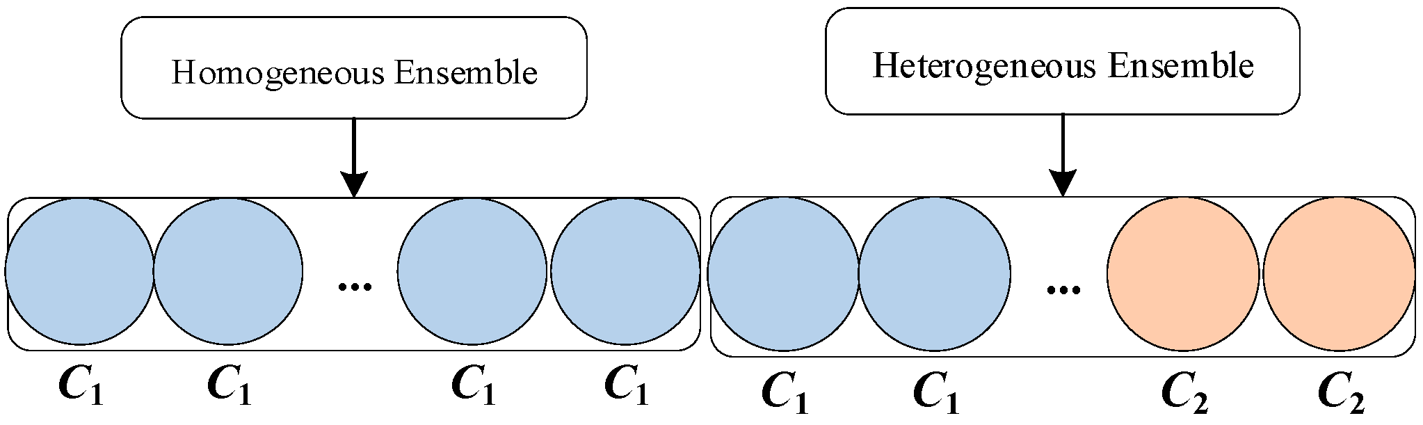
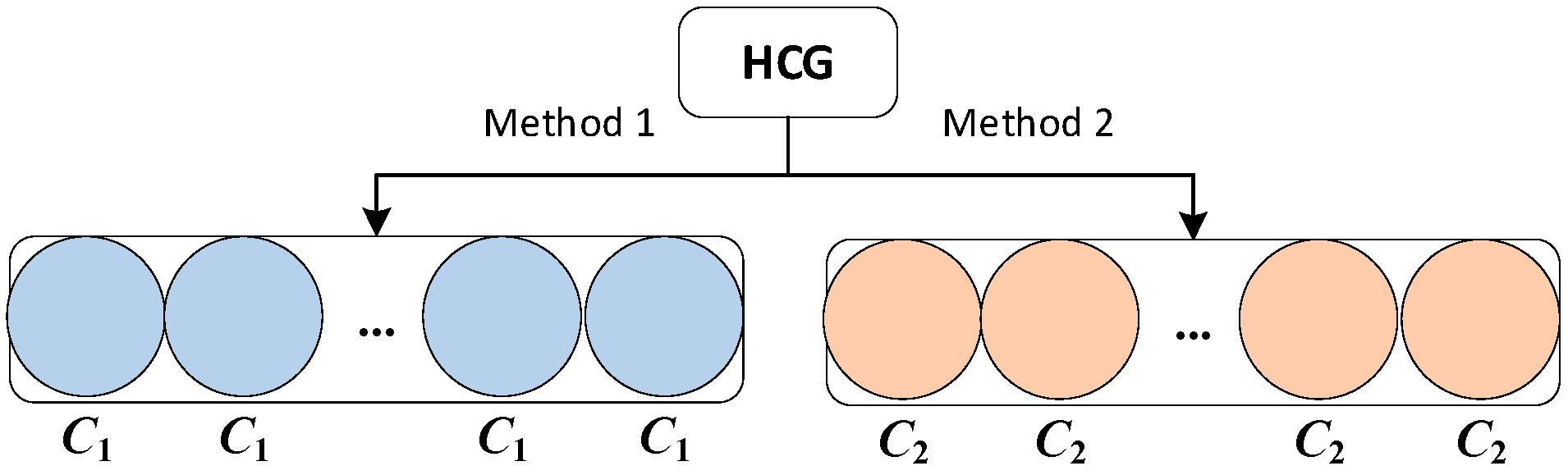
- The concept of a Heterogeneous Classifier Group is proposed. Two different ensemble classifiers are used in the testing and training stages. It is different from the previous concept of a heterogeneous ensemble, which is no longer an ensemble classifier with different kinds of base classifiers.
- (2)
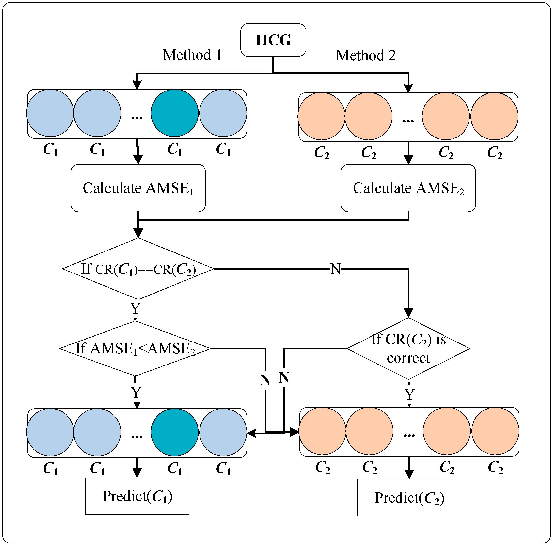
- The Adaptive Selection Strategy is proposed. It proposes to use the adaptive mean square error formula to calculate the sum of the error values of each group of ensemble classifiers and select the most suitable group of ensemble classifiers for testing by comparing the values.
- (3)
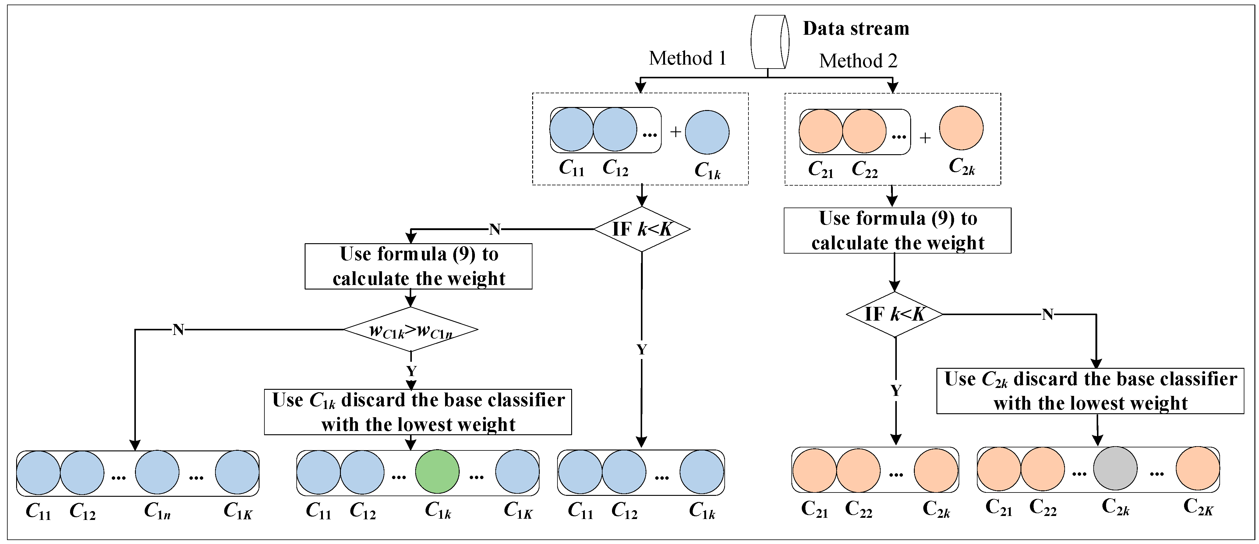
- The least squares method is used to calculate the weight of the base classifier in the Heterogeneous Classifier Group and dynamically update it according to the weight.
- (4)
- Experiments are carried out on seven real datasets, and the AHCG algorithm is compared with eight homogeneous ensemble methods. Good results are obtained in all four evaluation indexes.
2. Related Works
2.1. Classical Multi-Label Classification Algorithm
2.2. Multi-Label Classification of Single Algorithm
2.3. Ensemble Multi-Label Classification Algorithm
3. AHCG Algorithm
3.1. HCG Concept
3.2. Adaptive Selection Strategy
| Algorithm 1. AHCG |
| Input: D: data stream; DC: data block; K: number of integrated classifiers; M1, M2: set of ensemble classifiers |
|
|
|
|
|
|
|
|
|
|
|
|
|
|
|
|
3.3. Dynamic Update of Base Classifiers
| Algorithm 2. Train |
| Inputs: DC: data blocks; K: number of base classifiers; M: ensemble classifiers; C: base classifier |
| Output: ensemble classifiers |
|
|
|
|
|
|
|
|
3.4. Time Complexity Analysis
4. Experimental Results and Analysis
4.1. Experimental Settings
- (1)
- Datasets
- (2)
- Benchmark algorithm
- EBR [9]: An ensemble version of the BR model: each instance of BR is randomly generated, regardless of the relationship between labels;
- ECC [9]: An ensemble version of CCs, where the chain order of each CC is randomly generated; it takes into account global label dependencies;
- EPS [10]: An improved integrated version of LP pays attention to the most important relationships of labels by pruning the set of labels that appear less often;
- GORT [40]: Algorithm using iSOUP regression tree;
- EBRT [46]: A regression tree method for multi-label classification through multi-objective regression in stream setting;
- EaBR, EaCC, and EaPS [40]: Use ADWIN as their concept drift detector;
- MLSAMPkNN [20]: The algorithm uses self-adjusting memory penalty kNN;
- AESAKNNS [21]: The algorithm uses ensemble kNN;
- DHEML [43]: This algorithm is a heterogeneous ensemble algorithm and uses the Adaptive Selection Strategy.
- (3)
- Evaluation Metrics
4.2. Experimental Analysis
- (1)
- Comparative experiments of ensemble algorithms
- (2)
- Comparison with the classification of algorithms dealing with concept drift
- (3)
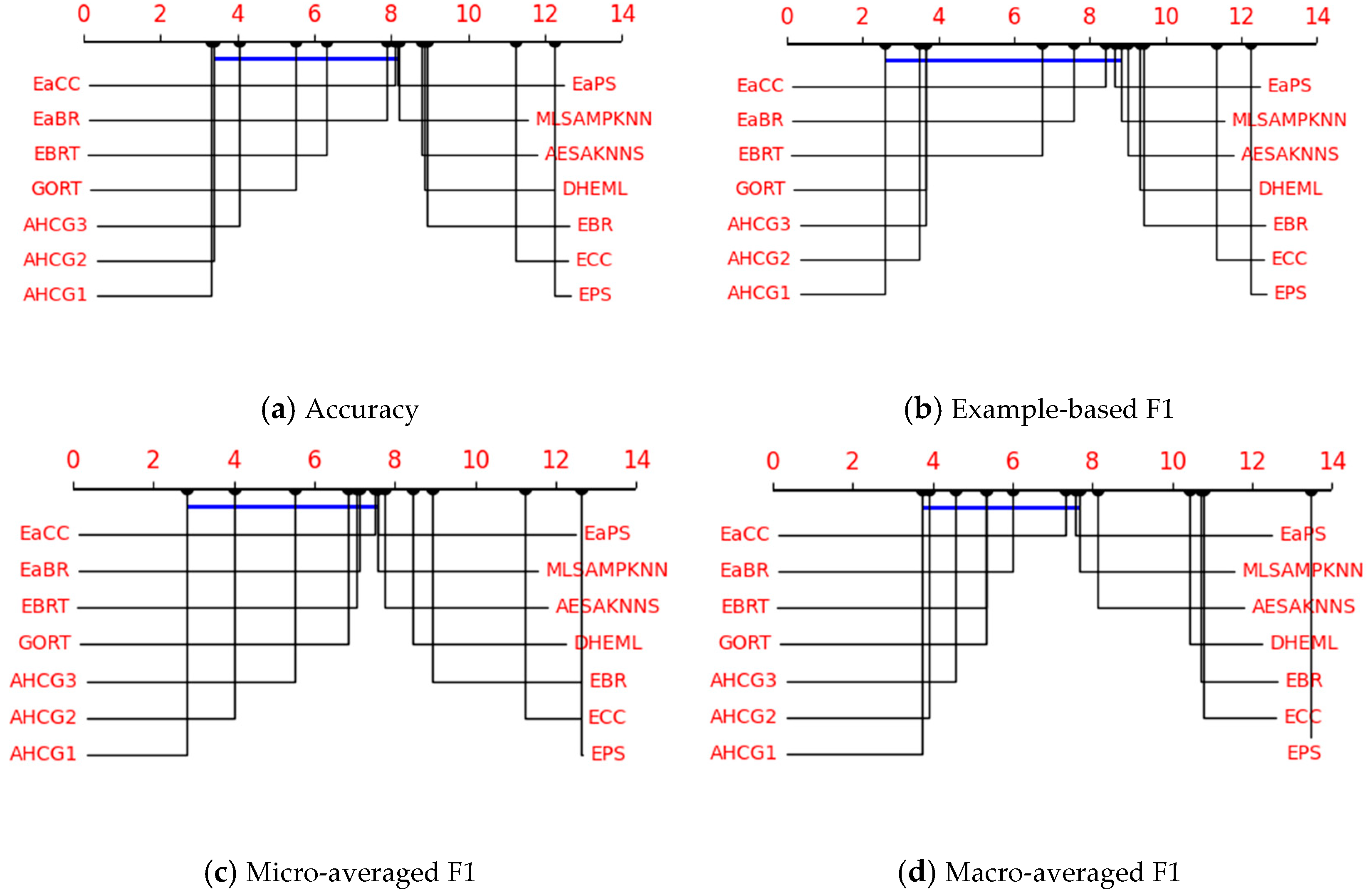
- Friedman statistical analysis
5. Summary
Author Contributions
Funding
Data Availability Statement
Conflicts of Interest
References
- Minaee, S.; Kalchbrenner, N.; Cambria, E.; Nikzad, N.; Chenaghlu, M.; Gao, J. Deep learning--based text classification: A comprehensive review. ACM Comput. Surv. (CSUR) 2021, 54, 1–40. [Google Scholar] [CrossRef]
- Liu, Q.; She, X.; Xia, Q. AI based diagnostics product design for osteosarcoma cells microscopy imaging of bone cancer patients using CA-MobileNet V3. J. Bone Oncol. 2024, 49, 100644. [Google Scholar] [CrossRef] [PubMed]
- Rana, P.; Meijering, E.; Sowmya, A.; Song, Y. Multi-Label Classification Based On Subcellular Region-Guided Feature Description for Protein Localisation. In Proceedings of the 18th International Symposium on Biomedical Imaging, Nice, France, 13–16 April 2021; pp. 1929–1933. [Google Scholar]
- Ding, Y.; Zhang, H.; Huang, W.; Zhou, X.; Shi, Z. Efficient Music Genre Recognition Using ECAS-CNN: A Novel Channel-Aware Neural Network Architecture. Sensors 2024, 24, 7021. [Google Scholar] [CrossRef] [PubMed]
- Xie, F.; Pan, X.; Yang, T.; Ernewein, B.; Li, M.; Robinson, D. A novel computer vision and point cloud-based approach for accurate structural analysis of a tall irregular timber structure. Structures 2024, 70, 107697. [Google Scholar] [CrossRef]
- Read, J.; Reutemann, P.; Pfahringer, B.; Holmes, G. Meka: A multi-label/multi-target extension to weka. J. Mach. Learn. Res. 2016, 17, 1–5. [Google Scholar]
- Osojnik, A.; Panov, P.; Džeroski, S. Multi-label classification via multi-target regression on data streams. Mach. Learn. 2017, 106, 745–770. [Google Scholar] [CrossRef]
- Duan, J.; Gu, Y.; Yu, H.; Yang, X.; Gao, S. ECC++: An algorithm family based on ensemble of classifier chains for classifying imbalanced multi-label data. Expert Syst. Appl. 2024, 236, 121366. [Google Scholar] [CrossRef]
- Mauri, L.; Damiani, E. Hardening behavioral classifiers against polymorphic malware: An ensemble approach based on minority report. Inf. Sci. 2025, 689, 121499. [Google Scholar] [CrossRef]
- Ganaie, M.; Hu, M.; Malik, A.; Tanveer, M.; Suganthan, P. Ensemble deep learning: A review. Eng. Appl. Artif. Intell. 2022, 115, 105151. [Google Scholar] [CrossRef]
- Alzubi, O.A.; Alzubi, J.A.; Alweshah, M.; Qiqieh, I.; Al-Shami, S.; Ramachandran, M. An optimal pruning algorithm of classifier ensembles: Dynamic programming approach. Neural Comput. Appl. 2020, 32, 16091–16107. [Google Scholar] [CrossRef]
- Tinofirei, M.; Fulufhelo, V.; Nelwamond, O.; Khmaies, O. An Adaptive Heterogeneous Online Learning Ensemble Classifier for Nonstationary Environments. Comput. Intell. Neurosci. 2021, 2021, 6669706. [Google Scholar]
- Hg, Z.; Altnay, H. Imbalance Learning Using Heterogeneous Ensembles. Expert Syst. Appl. 2019, 142, 113005. [Google Scholar]
- Read, J.; Martino, L.; Olmos, P.M.; Luengo, D. Scalable multi-output label prediction: From classifier chains to classifier trellises. Pattern Recognit. 2015, 48, 2096–2109. [Google Scholar] [CrossRef]
- Wang, R.; Kwong, S.; Wang, X.; Jia, Y. Active k-labelsets ensemble for multi-label classification. Pattern Recognit. 2021, 109, 107583. [Google Scholar] [CrossRef]
- Zhang, J.; Bian, Z.; Wang, S. Style linear k-nearest neighbor classification method. Appl. Soft Comput. 2024, 150, 111011. [Google Scholar] [CrossRef]
- Xiao, N.; Dai, S. A network big data classification method based on decision tree algorithm. Int. J. Reason.-Based Intell. Syst. 2024, 16, 66–73. [Google Scholar] [CrossRef]
- Zhang, Z.; Wang, Z.; Liu, H.; Sun, Y. Ensemble Multi-label Classification Algorithm Based on Tree-Bayesian Network. Comput. Sci. 2018, 45, 195–201. [Google Scholar]
- Roy, A.; Chakraborty, S. Support vector machine in structural reliability analysis: A review. Reliab. Eng. Syst. Saf. 2023, 233, 109126. [Google Scholar] [CrossRef]
- Kavitha, P.M.; Muruganantham, B. Mal_CNN: An Enhancement for Malicious Image Classification Based on Neural Network. Cybern. Syst. 2024, 55, 739–752. [Google Scholar] [CrossRef]
- Roseberry, M.; Krawczyk, B.; Cano, A. Multi-label punitive kNN with self-adjusting memory for drifting data streams. ACM Trans. Knowl. Discov. Data 2019, 13, 1–31. [Google Scholar] [CrossRef]
- Alberghini, G.; Junior, S.B.; Cano, A. Adaptive ensemble of self-adjusting nearest neighbor subspaces for multi-label drifting data streams. Neurocomputing 2022, 481, 228–248. [Google Scholar] [CrossRef]
- Rastin, N.; Jahromi, M.Z.; Taheri, M. Feature weighting to tackle label dependencies in multi-label stacking nearest neighbor. Appl. Intell. 2021, 51, 5200–5218. [Google Scholar] [CrossRef]
- Liu, C.; Cao, L. A coupled k-nearest neighbor algorithm for multi-label classification. In Proceedings of the Pacific-Asia Conference on Knowledge Discovery and Data Mining, Ho Chi Minh City, Vietnam, 19–22 May 2015; pp. 176–187. [Google Scholar]
- Luo, F.; Guo, W.; Yu, Y.; Chen, G. A multi-label classification algorithm based on kernel extreme learning machine. Neurocomputing 2017, 260, 313–320. [Google Scholar] [CrossRef]
- Rezaei, M.; Eftekhari, M.; Movahed, F.S. ML-CK-ELM: An efficient multi-layer extreme learning machine using combined kernels for multi-label classification. Sci. Iran. 2020, 27, 3005–3018. [Google Scholar] [CrossRef]
- Bezembinder, E.M.; Wismans LJ, J.; Berkum EC, V. Constructing multi-labelled decision trees for junction design using the predicted probabilities. In Proceedings of the 20th IEEE International Conference on Intelligent Transportation Systems, Yokohama, Japan, 16–19 October 2017; pp. 1–7. [Google Scholar]
- Majzoubi, M.; Choromanska, A. Ldsm: Logarithm-depth streaming multi-label decision trees. In Proceedings of the 23rd International Conference on Artificial Intelligence and Statistics, Online, 26–28 August 2020; pp. 4247–4257. [Google Scholar]
- Moral-García, S.; Mantas, C.J.; Castellano, J.G.; Abellán, J. Ensemble of classifier chains and credal C4.5 for solving multi-label classification. Prog. Artif. Intell. 2019, 8, 195–213. [Google Scholar] [CrossRef]
- Lotf, H.; Ramdani, M. Multi-Label Classification: A Novel approach using decision trees for learning Label-relations and preventing cyclical dependencies: Relations Recognition and Removing Cycles (3RC). In Proceedings of the 13th International Conference on Intelligent Systems: Theories and Applications, Rabat, Morocco, 23–24 September 2020; pp. 1–6. [Google Scholar]
- Nan, G.; Li, Q.; Dou, R.; Liu, J. Local positive and negative correlation-based k -labelsets for multi-label classification. Neurocomputing 2018, 318, 90–101. [Google Scholar] [CrossRef]
- Moyano, J.M.; Ventura, S. Auto-adaptive grammar-guided genetic programming algorithm to build ensembles of multi-label classifiers. Inf. Fusion 2022, 78, 1–19. [Google Scholar] [CrossRef]
- Mahdavi-Shahri, A.; Houshmand, M.; Yaghoobi, M.; Jalali, M. Applying an ensemble learning method for improving multi-label classification performance. In Proceedings of the 2nd International Conference of Signal Processing and Intelligent Systems, Tehran, Iran, 14–15 December 2016; pp. 1–62018. [Google Scholar]
- Moyano, J.M.; Gibaja, E.L.; Cios, K.J.; Ventura, S. Generating ensembles of multi-label classifiers using cooperative coevolutionary algorithms. In Proceedings of the 24th European Conference on Artificial Intelligence, Santiago de Compostela, Spain, 29 August–8 September 2020; pp. 1379–1386. [Google Scholar]
- Zhang, L.; Shah, S.K.; Kakadiaris, I.A. Hierarchical multi-label classification using fully associative ensemble learning. Pattern Recognit. 2017, 70, 89–103. [Google Scholar] [CrossRef]
- Wei, X.; Yu, Z.; Zhang, C.; Hu, Q. Ensemble of label specific features for multi-label classification. In Proceedings of the 2018 IEEE International Conference on Multimedia and Expo, San Diego, CA, USA, 23–27 July 2018; pp. 1–6. [Google Scholar]
- Cheng, K.; Gao, S.; Dong, W.; Yang, X.; Wang, Q.; Yu, H. Boosting label weighted extreme learning machine for classifying multi-label imbalanced data. Neurocomputing 2020, 403, 360–370. [Google Scholar] [CrossRef]
- Li, K.; Kong, X.; Lu, Z.; Wenyin, L.; Yin, J. Boosting weighted ELM for imbalanced learning. Neurocomputing 2014, 128, 15–21. [Google Scholar] [CrossRef]
- Büyükçakir, A.; Bonab, H.; Can, F. A novel online stacked ensemble for multi-label stream classification. In Proceedings of the 27th ACM International Conference on Information and Knowledge Management, Torino, Italy, 22–26 October 2018; pp. 1063–1072. [Google Scholar]
- Li, D.; Ji, L.; Liu, S. Research on sentiment classification method based on ensemble learning of heterogeneous classifiers. Eng. J. Wuhan Univ. 2021, 54, 975–982. [Google Scholar]
- Wu, D.; Han, B. Network Intrusion Detection Method Based on Optimization Heterogeneous Ensemble Learning of Glowworms. Fire Control Command Control 2021, 46, 26–31. [Google Scholar]
- Ding, J.; Wu, H.; Han, M. Multi-label data stream classification algorithm based on dynamic heterogeneous ensemble. Comput. Eng. Des. 2023, 44, 3031–3038. [Google Scholar]
- Singh, I.P.; Ghorbel, E.; Oyedotun, O.; Aouada, D. Multi-label image classification using adaptive graph convolutional networks: From a single domain to multiple domains. Comput. Vis. Image Underst. 2024, 247, 104062. [Google Scholar] [CrossRef]
- Brzezinski, D.; Stefanowski, J. Reacting to different types of concept drift: The accuracy updated ensemble algorithm. IEEE Trans. Neural Netw. Learn. Syst. 2013, 25, 81–94. [Google Scholar] [CrossRef] [PubMed]
- Bifet, A.; Holmes, G.; Pfahringer, B.; Read, J.; Kranen, P.; Kremer, H.; Jansen, T. MOA: A realtime analytics open source framework. In Machine Learning and Knowledge Discovery in Databases: European Conference, ECML PKDD 2011, Athens, Greece, 5–9 September 2011; Proceedings, Part III 22; Springer: Berlin/Heidelberg, Germany, 2011; pp. 617–620. [Google Scholar]
- Liu, J.; Xu, Y. T-Friedman test: A new statistical test for multiple comparison with an adjustable conservativeness measure. Int. J. Comput. Intell. Syst. 2022, 15, 29. [Google Scholar] [CrossRef]

| K | The number of base classifiers in the ensemble |
| n | The amount of data in the instance window |
| H | Maximum capacity of a data block DC |
| For the ith instance, the jth class label | |
| It is the weight of classifier k | |
| For the ith instance, the correlation score of the kth base classifier to the j class label | |
| S | Correlation score matrix; it obtains the predicted scores for different labels through different base classifiers |
| DC | A data stream is divided into blocks of data, DC = d1, d2, …, dh, …, dH |
| Algorithms | Time Complexity | Influence Factor |
|---|---|---|
| EBR | The number of iterations k, the number of labels p, and the training complexity of each binary classifier, etc. | |
| ECC | The number of iterations k, the number of labels p, and the training complexity of each binary classifier, etc. | |
| EPS | The number of iterations k, the size of the training set N, the number of labels p, and the pruning strategy, etc. | |
| GORT | The number of instances in DC n, the number of classifiers K, and the number of labels p, etc. | |
| EBRT | Dataset size N and number of features m, etc. | |
| EaBR | The number of instances in DC n, the number of classifiers K, and the number of labels p, etc. | |
| EaCC | The number of instances in DC n, the number of classifiers K, and the number of labels p, etc. | |
| EaPS | The number of instances in DC n, the number of classifiers K, and the number of labels p, etc. | |
| AHCG | The number of labels p and the number of classifiers K, etc. |
| Dataset | Domain | n | m | L | LC(D) | LD(D) |
|---|---|---|---|---|---|---|
| Medical | Text | 978 | 1449 | 45 | 1.245 | 0.028 |
| Enron | Text | 1702 | 1001 | 53 | 3.378 | 0.064 |
| Chess | Text | 1675 | 585 | 227 | 2.411 | 0.011 |
| Yeast | Biological | 2417 | 103 | 14 | 4.237 | 0.303 |
| Slashdot | Text | 3782 | 1079 | 22 | 1.18 | 0.053 |
| Philosophy | Text | 3971 | 842 | 233 | 2.272 | 0.010 |
| Reuters | Text | 6000 | 500 | 101 | 2.88 | 0.028 |
| chemistry | Text | 6961 | 540 | 175 | 2.109 | 0.012 |
| Cs | Text | 9270 | 635 | 274 | 2.556 | 0.009 |
| Ohsumed | Text | 13,930 | 1002 | 23 | 1.663 | 0.072 |
| TMC | Text | 28,600 | 500 | 22 | 2.158 | 0.098 |
| IDBI | Text | 120,900 | 1001 | 28 | 2.000 | 0.071 |
| Symbol | Meaning |
|---|---|
| d dimensional instance space | |
| it marks the space with q possible category labels, {} | |
| x | d dimensional eigenvector, (x1, x2, …, xd) (x∈) |
| p | p indicates the number of instances. 1 ≤ i ≤ p |
| Y | a set of labels associated with X (Y⊆Y) |
| h(∙) | MLC h: →, where h(x) returns the correct set of labels for x |
| Evaluation Metrics | Date Set | AHCG1 | AHCG2 | AHCG3 | EBR | ECC | EPS | DHEML |
|---|---|---|---|---|---|---|---|---|
| Accuracy | Medical | 0.271 | 0.272 | 0.286 | 0.193 | 0.189 | 0.205 | 0.285 |
| Enron | 0.322 | 0.172 | 0.322 | 0.342 | 0.298 | 0.302 | 0.304 | |
| Chess | 0.056 | 0.075 | 0.086 | 0.067 | 0.062 | 0.053 | 0.079 | |
| Yeast | 0.51 | 0.505 | 0.508 | 0.502 | 0.493 | 0.48 | 0.513 | |
| Philosophy | 0.029 | 0.087 | 0.033 | 0.013 | 0.011 | 0.072 | 0.072 | |
| Chemistry | 0.058 | 0.069 | 0.058 | 0.022 | 0.015 | 0.02 | 0.061 | |
| Cs | 0.056 | 0.074 | 0.086 | 0.067 | 0.062 | 0.053 | 0.071 | |
| Slashdot | 0.073 | 0.133 | 0.076 | 0.02 | 0.018 | 0.07 | 0.114 | |
| Reuters | 0.078 | 0.154 | 0.136 | 0.099 | 0.093 | 0.131 | 0.154 | |
| Ohsumed | 0.264 | 0.212 | 0.275 | 0.191 | 0.18 | 0.135 | 0.245 | |
| TMC | 0.504 | 0.499 | 0.511 | 0.52 | 0.511 | 0.469 | 0.502 | |
| IDBI | 0.163 | 0.172 | 0.164 | 0.055 | 0.012 | 0.011 | 0.166 | |
| Rank. avg | 4.17 | 2.88 | 2.38 | 2.50 | 4.42 | 5.88 | 5.79 | |
| Example-Based F1 | Medical | 0.3 | 0.341 | 0.315 | 0.216 | 0.21 | 0.235 | 0.329 |
| Enron | 0.462 | 0.264 | 0.462 | 0.468 | 0.414 | 0.397 | 0.460 | |
| Chess | 0.128 | 0.138 | 0.2 | 0.095 | 0.087 | 0.079 | 0.182 | |
| Yeast | 0.648 | 0.639 | 0.645 | 0.638 | 0.632 | 0.601 | 0.647 | |
| Philosophy | 0.087 | 0.156 | 0.104 | 0.018 | 0.015 | 0.072 | 0.141 | |
| chemistry | 0.15 | 0.143 | 0.15 | 0.03 | 0.02 | 0.026 | 0.134 | |
| Cs | 0.128 | 0.137 | 0.203 | 0.095 | 0.087 | 0.079 | 0.168 | |
| Slashdot | 0.118 | 0.199 | 0.12 | 0.023 | 0.02 | 0.075 | 0.171 | |
| Reuters | 0.143 | 0.241 | 0.226 | 0.106 | 0.099 | 0.136 | 0.227 | |
| Ohsumed | 0.383 | 0.344 | 0.389 | 0.23 | 0.217 | 0.16 | 0.342 | |
| TMC | 0.656 | 0.65 | 0.666 | 0.654 | 0.643 | 0.59 | 0.644 | |
| IDBI | 0.288 | 0.294 | 0.289 | 0.075 | 0.016 | 0.015 | 0.135 | |
| Rank. avg | 3.00 | 2.67 | 2.08 | 2.92 | 4.83 | 6.33 | 6.17 | |
| Micro-Averaged F1 | Medical | 0.613 | 0.703 | 0.636 | 0.497 | 0.489 | 0.396 | 0.564 |
| Enron | 0.449 | 0.244 | 0.449 | 0.403 | 0.191 | 0.358 | 0.436 | |
| Chess | 0.034 | 0.123 | 0.031 | 0.122 | 0.115 | 0.11 | 0.120 | |
| Yeast | 0.638 | 0.639 | 0.636 | 0.631 | 0.625 | 0.604 | 0.638 | |
| Philosophy | 0.02 | 0.127 | 0.02 | 0.022 | 0.019 | 0.098 | 0.086 | |
| chemistry | 0.027 | 0.095 | 0.014 | 0.04 | 0.028 | 0.034 | 0.053 | |
| Cs | 0.032 | 0.123 | 0.029 | 0.122 | 0.115 | 0.11 | 0.119 | |
| Slashdot | 0.11 | 0.199 | 0.111 | 0.041 | 0.037 | 0.106 | 0.157 | |
| Reuters | 0.041 | 0.207 | 0.041 | 0.143 | 0.135 | 0.154 | 0.153 | |
| Ohsumed | 0.283 | 0.307 | 0.295 | 0.294 | 0.28 | 0.197 | 0.283 | |
| TMC | 0.618 | 0.61 | 0.632 | 0.638 | 0.631 | 0.566 | 0.621 | |
| IDBI | 0.215 | 0.279 | 0.216 | 0.099 | 0.014 | 0.018 | 0.225 | |
| Rank.avg | 4.54 | 1.83 | 4.21 | 3.00 | 3.67 | 5.58 | 5.17 | |
| Macro-Averaged F1 | Medical | 0.033 | 0.035 | 0.034 | 0.028 | 0.028 | 0.021 | 0.035 |
| Enron | 0.07 | 0.06 | 0.07 | 0.05 | 0.046 | 0.034 | 0.056 | |
| Chess | 0.021 | 0.019 | 0.028 | 0.037 | 0.032 | 0.006 | 0.025 | |
| Yeast | 0.368 | 0.353 | 0.356 | 0.329 | 0.343 | 0.343 | 0.363 | |
| Philosophy | 0.019 | 0.012 | 0.02 | 0.012 | 0.007 | 0.005 | 0.015 | |
| chemistry | 0.027 | 0.062 | 0.027 | 0.02 | 0.012 | 0.004 | 0.023 | |
| Cs | 0.021 | 0.02 | 0.027 | 0.037 | 0.032 | 0.006 | 0.027 | |
| Slashdot | 0.096 | 0.162 | 0.097 | 0.039 | 0.036 | 0.077 | 0.139 | |
| Reuters | 0.037 | 0.072 | 0.039 | 0.057 | 0.049 | 0.021 | 0.053 | |
| Ohsumed | 0.236 | 0.28 | 0.255 | 0.244 | 0.23 | 0.082 | 0.251 | |
| TMC | 0.432 | 0.421 | 0.491 | 0.485 | 0.465 | 0.199 | 0.488 | |
| IDBI | 0.115 | 0.137 | 0.115 | 0.032 | 0.014 | 0.029 | 0.118 | |
| Rank. avg | 3.71 | 3.00 | 2.67 | 2.83 | 4.08 | 5.08 | 6.63 |
| Running Time | AHCG1 | AHCG2 | AHCG3 | EBR | ECC | EPS | DHEML |
|---|---|---|---|---|---|---|---|
| Medical | 54,480 | 53,312 | 95,348 | 384,636 | 390,410 | 7019 | 65,695 |
| Enron | 330,011 | 296,226 | 545,682 | 634,480 | 623,481 | 17,758 | 378,999 |
| Chess | 40,317,450 | 53,310,855 | 85,347,953 | 28,946,030 | 21,725,172 | 160,898 | 57,880,922 |
| Yeast | 27,138 | 28,007 | 37,427 | 29,333 | 31,378 | 4545 | 29,938 |
| Philosophy | 10,513,191 | 11,601,136 | 21,001,456 | 10,956,341 | 8,151,044 | 88,600 | 13,943,644 |
| chemistry | 9,525,265 | 13,239,025 | 21,925,773 | 7,708,541 | 6,474,030 | 87,881 | 14,452,766 |
| Cs | 45,607,460 | 69,042,003 | 113,073,438 | 35,952,832 | 29,460,820 | 196,050 | 73,645,586 |
| Slashdot | 572,558 | 584,341 | 857,543 | 544,816 | 560,608 | 95,291 | 651,471 |
| Reuters | 2,858,115 | 2,622,387 | 5,223,701 | 2,097,796 | 2,124,155 | 48,777 | 3,461,739 |
| Ohsumed | 4,223,451 | 3,963,728 | 5,874,063 | 2,320,674 | 2,468,183 | 289,888 | 4,547,406 |
| TMC | 4,341,980 | 4,309,034 | 6,791,509 | 2,273,091 | 2,490,216 | 111,747 | 4,994,112 |
| IDBI | 115,513,788 | 100,334,992 | 180,692,563 | 67,979,363 | 71,315,269 | 1,658,930 | 128,241,470 |
| Evaluation Metrics | Dataset | AHCG1 | AHCG2 | AHCG2 | GORT | EBRT | EaBR | EaCC | EaPS | MLSAMPKNN | AESAKNNS | DHEML |
|---|---|---|---|---|---|---|---|---|---|---|---|---|
| Accuracy | Medical | 0.271 | 0.272 | 0.286 | 0.197 | 0.279 | 0.192 | 0.189 | 0.209 | 0.075 | 0.112 | 0.285 |
| Enron | 0.322 | 0.172 | 0.322 | 0.213 | 0.059 | 0.308 | 0.289 | 0.26 | 0294 | 0.327 | 0.304 | |
| Chess | 0.056 | 0.075 | 0.086 | 0.03 | 0 | 0.064 | 0.003 | 0.028 | 0.03 | 0.043 | 0.079 | |
| Yeast | 0.51 | 0.505 | 0.508 | 0.464 | 0.502 | 0.502 | 0.495 | 0.474 | 0.456 | 0.271 | 0.513 | |
| Philosophy | 0.029 | 0.087 | 0.033 | 0.032 | 0 | 0.012 | 0.003 | 0.057 | 0.022 | 0.037 | 0.072 | |
| chemistry | 0.058 | 0.069 | 0.058 | 0.035 | 0 | 0.013 | 0.001 | 0.019 | 0.039 | 0.026 | 0.061 | |
| Cs | 0.056 | 0.074 | 0.086 | 0.03 | 0 | 0.064 | 0.003 | 0.028 | 0.03 | 0.03 | 0.071 | |
| Slashdot | 0.073 | 0.133 | 0.076 | 0.11 | 0.001 | 0.016 | 0.018 | 0.044 | 0.221 | 0.135 | 0.114 | |
| Reuters | 0.078 | 0.154 | 0.136 | 0.041 | 0.000 | 0.051 | 0.004 | 0.17 | 0.289 | 0.262 | 0.154 | |
| Ohsumed | 0.264 | 0.212 | 0.275 | 0.179 | 0.049 | 0.169 | 0.004 | 0.113 | 0.069 | 0.001 | 0.245 | |
| TMC | 0.504 | 0.499 | 0.511 | 0.295 | 0.007 | 0.529 | 0.516 | 0.481 | 0.177 | 0.214 | 0.502 | |
| IDBI | 0.163 | 0.172 | 0.164 | 0.162 | 0.000 | 0.024 | 0.001 | 0.019 | 0.155 | 0.133 | 0.166 | |
| Rank. avg | 4.58 | 3.63 | 3.08 | 6.96 | 9.71 | 6.46 | 8.67 | 7.08 | 6.29 | 6.50 | 3.04 | |
| Example-Based F1 | Medical | 0.3 | 0.341 | 0.315 | 0.286 | 0.321 | 0.214 | 0.21 | 0.24 | 0.085 | 0.132 | 0.329 |
| Enron | 0.462 | 0.264 | 0.462 | 0.35 | 0.061 | 0.425 | 0.408 | 0.347 | 0.391 | 0.445 | 0.46 | |
| Chess | 0.128 | 0.138 | 0.200 | 0.057 | 0 | 0.091 | 0.005 | 0.04 | 0.03 | 0.047 | 0.182 | |
| Yeast | 0.648 | 0.639 | 0.645 | 0.614 | 0.638 | 0.638 | 0.633 | 0.596 | 0.586 | 0.373 | 0.647 | |
| Philosophy | 0.087 | 0.156 | 0.104 | 0.063 | 0 | 0.017 | 0.004 | 0.073 | 0.049 | 0.029 | 0.141 | |
| chemistry | 0.15 | 0.143 | 0.15 | 0.068 | 0 | 0.017 | 0.001 | 0.024 | 0.052 | 0.034 | 0.134 | |
| Cs | 0.128 | 0.137 | 0.203 | 0.058 | 0 | 0.091 | 0.005 | 0.04 | 0.045 | 0.043 | 0.168 | |
| Slashdot | 0.118 | 0.199 | 0.12 | 0.194 | 0.001 | 0.018 | 0.02 | 0.047 | 0.23 | 0.138 | 0.171 | |
| Reuters | 0.143 | 0.241 | 0.226 | 0.08 | 0.000 | 0.055 | 0.005 | 0.176 | 0.311 | 0.279 | 0.227 | |
| Ohsumed | 0.383 | 0.344 | 0.389 | 0.298 | 0.056 | 0.202 | 0.005 | 0.134 | 0.09 | 0.001 | 0.342 | |
| TMC | 0.656 | 0.65 | 0.666 | 0.449 | 0.008 | 0.661 | 0.646 | 0.598 | 0.196 | 0.236 | 0.644 | |
| IDBI | 0.288 | 0.294 | 0.289 | 0.28 | 0.000 | 0.031 | 0.001 | 0.026 | 0.206 | 0.17 | 0.135 | |
| Rank. avg | 3.58 | 3.17 | 2.50 | 6.08 | 9.71 | 6.79 | 8.83 | 7.67 | 6.83 | 7.33 | 3.50 | |
| Micro-Averaged F1 | Medical | 0.613 | 0.703 | 0.636 | 0.209 | 0.432 | 0.493 | 0.037 | 0.402 | 0.202 | 0.293 | 0.564 |
| Enron | 0.449 | 0.244 | 0.449 | 0.345 | 0.037 | 0.411 | 0.395 | 0.33 | 0.384 | 0.443 | 0.436 | |
| Chess | 0.034 | 0.123 | 0.031 | 0.057 | 0 | 0.116 | 0.007 | 0.051 | 0.045 | 0.063 | 0.12 | |
| Yeast | 0.638 | 0.639 | 0.636 | 0.602 | 0.632 | 0.632 | 0.627 | 0.6 | 0.587 | 0.42 | 0.638 | |
| Philosophy | 0.02 | 0.127 | 0.02 | 0.062 | 0 | 0.021 | 0.006 | 0.081 | 0.055 | 0.037 | 0.086 | |
| chemistry | 0.027 | 0.095 | 0.014 | 0.067 | 0 | 0.023 | 0.001 | 0.024 | 0.061 | 0.044 | 0.053 | |
| CS | 0.032 | 0.123 | 0.029 | 0.057 | 0 | 0.116 | 0.007 | 0.051 | 0.058 | 0.059 | 0.119 | |
| Slashdot | 0.11 | 0.199 | 0.111 | 0.191 | 0.001 | 0.033 | 0.037 | 0.074 | 0.268 | 0.204 | 0.157 | |
| Reuters | 0.041 | 0.207 | 0.041 | 0.079 | 0.000 | 0.076 | 0.007 | 0.2 | 0.342 | 0.331 | 0.153 | |
| Ohsumed | 0.283 | 0.307 | 0.295 | 0.271 | 0.076 | 0.266 | 0.007 | 0.171 | 0.114 | 0.002 | 0.283 | |
| TMC | 0.618 | 0.61 | 0.632 | 0.435 | 0.008 | 0.64 | 0.632 | 0.577 | 0.351 | 0.405 | 0.621 | |
| IDBI | 0.215 | 0.279 | 0.216 | 0.273 | 0.000 | 0.041 | 0.002 | 0.033 | 0.218 | 0.201 | 0.225 | |
| Rank. avg | 5.63 | 2.50 | 5.58 | 5.58 | 9.96 | 5.71 | 8.79 | 6.92 | 5.92 | 6.00 | 3.42 | |
| Macro-Averaged F1 | Medical | 0.033 | 0.035 | 0.034 | 0.023 | 0.016 | 0.028 | 0.028 | 0.021 | 0.01 | 0.015 | 0.035 |
| Enron | 0.07 | 0.06 | 0.07 | 0.095 | 0.006 | 0.065 | 0.062 | 0.045 | 0.127 | 0.148 | 0.056 | |
| Chess | 0.021 | 0.019 | 0.028 | 0.023 | 0 | 0.023 | 0.002 | 0.004 | 0.012 | 0.027 | 0.025 | |
| Yeast | 0.368 | 0.353 | 0.356 | 0.357 | 0.329 | 0.329 | 0.346 | 0.341 | 0.379 | 0.194 | 0.363 | |
| Philosophy | 0.019 | 0.012 | 0.02 | 0.02 | 0 | 0.011 | 0.002 | 0.004 | 0.006 | 0.013 | 0.015 | |
| chemistry | 0.027 | 0.062 | 0.027 | 0.027 | 0 | 0.012 | 0.000 | 0.003 | 0.009 | 0.013 | 0.023 | |
| Cs | 0.021 | 0.02 | 0.027 | 0.022 | 0 | 0.035 | 0.002 | 0.004 | 0.012 | 0.025 | 0.027 | |
| Slashdot | 0.096 | 0.162 | 0.097 | 0.115 | 0.000 | 0.033 | 0.036 | 0.041 | 0.136 | 0.084 | 0.139 | |
| Reuters | 0.037 | 0.072 | 0.039 | 0.042 | 0.000 | 0.028 | 0.004 | 0.03 | 0.163 | 0.162 | 0.053 | |
| Ohsumed | 0.236 | 0.28 | 0.255 | 0.219 | 0.028 | 0.215 | 0.006 | 0.065 | 0.052 | 0.001 | 0.251 | |
| TMC | 0.432 | 0.421 | 0.491 | 0.277 | 0.003 | 0.481 | 0.462 | 0.329 | 0.06 | 0.09 | 0.488 | |
| IDBI | 0.115 | 0.137 | 0.115 | 0.132 | 0.000 | 0.013 | 0.002 | 0.027 | 0.107 | 0.104 | 0.118 | |
| Rank. avg | 4.58 | 4.04 | 3.25 | 4.33 | 10.50 | 6.46 | 8.58 | 8.33 | 6.17 | 6.25 | 3.50 |
Disclaimer/Publisher’s Note: The statements, opinions and data contained in all publications are solely those of the individual author(s) and contributor(s) and not of MDPI and/or the editor(s). MDPI and/or the editor(s) disclaim responsibility for any injury to people or property resulting from any ideas, methods, instructions or products referred to in the content. |
© 2024 by the authors. Licensee MDPI, Basel, Switzerland. This article is an open access article distributed under the terms and conditions of the Creative Commons Attribution (CC BY) license (https://creativecommons.org/licenses/by/4.0/).
Share and Cite
Han, M.; Yang, S.; Wu, H.; Ding, J. Multi-Label Classification Algorithm for Adaptive Heterogeneous Classifier Group. Mathematics 2025, 13, 103. https://doi.org/10.3390/math13010103
Han M, Yang S, Wu H, Ding J. Multi-Label Classification Algorithm for Adaptive Heterogeneous Classifier Group. Mathematics. 2025; 13(1):103. https://doi.org/10.3390/math13010103
Chicago/Turabian StyleHan, Meng, Shurong Yang, Hongxin Wu, and Jian Ding. 2025. "Multi-Label Classification Algorithm for Adaptive Heterogeneous Classifier Group" Mathematics 13, no. 1: 103. https://doi.org/10.3390/math13010103
APA StyleHan, M., Yang, S., Wu, H., & Ding, J. (2025). Multi-Label Classification Algorithm for Adaptive Heterogeneous Classifier Group. Mathematics, 13(1), 103. https://doi.org/10.3390/math13010103