Adaptive RBF Neural Network Tracking Control of Stochastic Nonlinear Systems with Actuators and State Constraints

Abstract

This paper investigates the adaptive neural network (NN) tracking control problem for stochastic nonlinear systems with multiple actuator constraints and full-state constraints. The issue of system full-state constraints is tackled by a generalized barrier Lyapunov function (GBLF), and the output constraints of the system are considered to be in the form of time-varying functions, which are more in line with the needs of real physical systems. The NN approximation technique is utilized to overcome the influence of the uncertainty term on controller design due to randomness. Based on the backstepping technique, a neural adaptive fixed-time tracking control strategy is designed. Under the designed control strategy, the tracking accuracy of the controlled system can reach the expectation in a fixed time. The multi-actuator constraints are converted into a generalized mathematical model to simplify the controller design process. Using the characteristics of the hyperbolic tangent function, a new function called practical virtual control signal is designed using the virtual control signal as the input. Due to the saturation constraint property of the hyperbolic tangent function, it is theoretically ensured that no state of the system exceeds the constraints through to the new form of the virtual controller. Using the adaptive controller constructed in this paper, the controlled system is semi-global fixed-time stabilized in probability (SGFSP). Finally, the effectiveness of the proposed control strategy is further verified by simulation examples.

1. Introduction

The control and tracking theory of uncertain nonlinear systems has been extensively developed in the last two decades and occupies an essential place in many applications, such as unmanned aerial systems [1,2,3], electromechanical systems [4,5], and robotic systems [6,7,8]. The existence of uncertainty in nonlinear systems makes the construction of controllers a difficult and important task, and stochastic nonlinear systems, as a special case of uncertain nonlinear systems, have also attracted much attention [9,10]. The backstepping method is a practical approach to nonlinear control problems, and was proposed by Krstic, Kanellakopoulos, and Kokotovic at the end of the last century [11]. Combining the backstepping method with a fuzzy or neural adaptive technique yields an effective control tool for solving uncertain nonlinear systems [12,13,14]. Due to the characteristics of the adaptive backstepping method, it is possible to achieve asymptotic sedimentation of nonlinear systems and guarantee boundedness of the signal under parameter uncertainty, which has led to many fruitful results [15,16,17]. Researchers have [18] investigated the robust adaptive control of non-triangular stochastic nonlinear systems. The neural adaptive finite-time control (FTC) technique is widely used as it allows the controlled system to achieve good tracking performance in finite time [19,20,21].

However, all of the above research results contain a common distinctive trait, which is that the finite time control method has this serious drawback while having good control performance. The establishment time of the controlled system utilizing the FTC strategy is directly related to the initial conditions of the controlled system and is positively related to the deviation of the initial state and the equilibrium point [22]. A more important point is that the preliminary conditions for many real industrial physical systems are hardly directly accessible. In contrast, using the fixed-time control strategy, the establishment time of the controlled system is independent of the preliminary conditions of the system, which can be predicted by the system and controller parameters, and this has led to the emergence of many excellent fixed-time control results [23,24,25]. Compared with the FTC strategy, the fixed-time control method can achieve stabilization in the state of unknown initial parameters in a predicted time and has better control performance.

Notice that real systems will always have various nonlinear constraints, which include input saturation, input deadband, and state constraints. The presence of these nonlinear constraints reduces the performance of the controlled system and affects the stability of the system. Therefore, much work has been conducted to solve the problems posed by these nonlinear constraints [26,27,28]. Reference [26] investigates the problem of adaptive full-state constrained control for stochastic nonlinear systems with unknown virtual control systems. The adaptive fixed-time control problem for stochastic nonlinear systems with state constraints and input saturation is studied in Reference [27]. Reference [28] considers the problem of tracking control for a class of state-constrained stochastic nonlinear systems with parameter uncertainty and input saturation. Unfortunately, the constraints on the output of the system are fixed value constraints rather than time-varying function constraints.

The time-varying function constraints for the controlled system have more stringent conditions compared to the constraints with fixed values and are more in line with the reality of real physical systems. In the case of the obstacle Lyapunov function, the time-varying function type of the bounds corresponds to an additional complexity term when obtaining the time derivative in relation to it, which greatly increases the subsequent process of controller design.

Note that almost all control strategies on state constraints are designed based on backstepping methods. When using the backstepping method for controller design, corresponding to the state constraint $∥x_i∥<L_i$, the virtual error is defined as $z_i=x_i-{\alpha }_{i-1}$, where ${\alpha }_{i-1}$ is the virtual controller built for the $\left(i-1\right)$th subsystem. In order to accomplish the task of state constraints using the barrier Lyapunov technique, it is generally necessary to determine the constraints on the virtual error $∥z_i∥<H_i=L_i-∥{\alpha }_{i-1}∥$. However, the following problems arise with this approach. We need to ensure that the virtual controller ${\alpha }_{i-1}$ satisfies the constraints of the corresponding state $x_i$, i.e., $∥{\alpha }_{i-1}∥<L_i$, otherwise, the above equation will be meaningless because $H_i\le 0$. However, to avoid the above problems, existing literature often assumes that the virtual controller satisfies the corresponding constraints. This paper will challenge the solution to the above paradoxical problem concerning virtual controllers in the context of tracking control problems for stochastic nonlinear systems subject to time-varying state constraints.

In summary, it is an interesting task to explore the fixed-time control problem for fully constrained stochastic nonlinear systems. In order to obtain more practically meaningful control schemes for stochastic nonlinear systems, this paper will consider both multi-actuator constraints and time-varying constraints on the system output. Compared with the current research results, the main contributions can be summarized as follows:

• Compared with the existing stochastic nonlinear systems with fixed numerical constraints on the system output, the control strategy designed in this paper ensures that the system output satisfies the time-varying function constraints, which is more in line with the state requirements of the actual physical system.
• By using the properties of the hyperbolic tangent function, this paper ensures that the intermediate virtual controllers required to realize the control task also meet the corresponding constraints. It is mathematically ensured that any state of the controlled system satisfies the constraint requirements at any moment.
• With the control method used in this paper, the control inputs and intermediate states are consistent with the constraints, which meets the realistic requirements of the actual physical control process, and the output tracking error can be quickly converged to within a bounded and adjustable tight set in fixed time.

The rest of this paper is described below. Section 2 provides an introduction to the problem description and preparatory knowledge. Section 3 presents controller design and stability analysis. Section 4 presents the simulations and the result analysis. Finally, Section 5 analyzes and concludes the paper.

2. Preliminaries

In this section, the system model, neural network, and preparatory knowledge are described. The main symbols used in this paper are shown in Table 1.

Table 1. Notations.

Symbol	Definition	Symbol	Definition
$\left|\ast \right|$	Absolute value	$\mathsf{\Omega }$	Sample space
${\mathsf{\Omega }}_0$	Compact set around zero	$\mathsf{\Pi }$	$\sigma$-algebra
P	The probability measure	$x^T$	The transpose of matrix x
$E\left\{\ast \right\}$	The mathematical expectation of ∗	$R^{+}$	Set of non-negative real numbers
$∥\ast ∥$	The Euclidean or Frobenius norm	$R^n$	Real n-dimension space
$C^i$	The set of i-times continuous differentiable functions

For simplicity, all variables x in this paper denote the function $x\left(t\right)$.

2.1. Stochastic Theory

Consider a $It\widehat{o}$ stochastic nonlinear system

$$dx=g\left(t,x\right)dt+f\left(t,x\right)d\omega \left(t\right),\forall x_0=x\left(0\right)\in R^n,t\ge 0$$

(1)

where $x\in R^n$ indicates the system state, $g:R^{+}\times R^n\to R^n,f:R^{+}\times R^n\to R^{n\times m}$, and $\omega$ illustrates the m-dimensional standard Wiener process defined on a complete probability space $\left(\mathsf{\Omega },\mathsf{\Pi },P\right)$. The associated stochastic settling time function is denoted as $T\left(x_0,\omega \right)=inf\left\{t\ge 0\left|x\left(t,x_0\right)\in {\mathsf{\Omega }}_0\right.\right\}$, which is the first time at which it arrives at ${\mathsf{\Omega }}_0$. To continue with the design of the control scheme in this paper, the following definitions are given with reference to article [29,30,31].

Definition 1.

As for system (1) and a Lyapunov function $V\left(x\right)\in C^2\left(R^n\right)$, the infinitesimal generator L can be expressed as follows:

$$LV\left(x\right)=\frac{\partial V}{\partial x}g(t,x)+\frac{1}{2}Tr\left\{f^T(t,x)\frac{{\partial }^{2}V}{\partial x^2}f(t,x)\right\}$$

(2)

where $Tr\left(\blacksquare \right)$ indicates the trace for the matrix.

Definition 2.

System (1) is said to be SGFSP, if, for any initial state $x_0\in R^n$ and a given positive constant $T_{max}>0$, the following statements hold:

1.

The system is semi-globally finite-time stable in probability.

2.

Mathematical expectation of the settling time function $T\left(x_0,\varpi \right)$ is bounded and the upper bound is a positive constant $T_{max}$, which is independent of the initial state of system (1). That is to say, $E\left(T\left(x_0,\omega \right)\right)\le T_{max},\forall x_0\in R^n$.

Remark 1.

The fixed time stability theory can be given by the above definition. The setting time of the fixed-time control strategy can be independent of the initial state, which has better tracking error convergence performance.

2.2. Related Lemmas

Lemma 1

([32]). For any real variables $\zeta \in R$ and a positive constant ε, the following inequality holds

$$0\le \left|\zeta \right|-\zeta tanh\left(\frac{\zeta }{\tau }\right)\le \varsigma \tau$$

(3)

in which $\varsigma =0.2785$.

Lemma 2

([33]). For $x_i>0$ and the positive real number ρ, the following inequality holds

$${\left(\sum _{i=1}^n{x}_i\right)}^{\rho }\le max\left\{n^{\rho -1},1\right\}\sum _{i=1}^n{x}_i^{\rho }$$

(4)

Lemma 3

([34]). For any positive real numbers $b_1,b_2,b_3$ and real variable $x,y$, the below inequality holds

$${\left|x\right|}^{b_1}{\left|y\right|}^{b_2}\le \frac{b_1}{b_1+b_2}{b}_3{\left|x\right|}^{b_1+b_2}+\frac{b_2}{b_1+b_2}{b}_3^{-\frac{b_1}{b_2}}{\left|y\right|}^{b_1+b_2}$$

(5)

Lemma 4

([27]). Regarding the stochastic nonlinear system (1), for any $x_0\in R^n$ and $\forall t\ge 0$, if the function $V\left(x\right)\in R^{+}$ is positive definite, and the ${\kappa }_{\infty }$ class functions ${\xi }_1$ and ${\xi }_2$, and normal numbers $c_1,c_2,\delta ,0<{\rho }_1<1$, and ${\rho }_2>1$ meet

$$\left\{\begin{array}{cc}\hfill & {\xi }_1\left(∥x∥\right)\le V\left(x\right)\le {\xi }_2\left(∥x∥\right)\hfill \\ \hfill & LV\left(x\right)\le -c_1{V}^{{\rho }_1}\left(x\right)-c_2{V}^{{\rho }_2}\left(x\right)+\delta \hfill \end{array}\right.$$

(6)

Then, we can say that the stochastic system (1) is SGFSP, and the settling time function is expressed as follows:

$$\begin{array}{cc}\hfill & E\left(T\right)\le T_{max}=max\left\{\frac{1}{c_1\mu (1-{\rho }_1)}+\frac{1}{c_2({\rho }_2-1)},\right.\hfill \\ \hfill & \left.\frac{1}{c_1(1-{\rho }_1)}+\frac{1}{c_2\mu ({\rho }_2-1)}\right\}\hfill \end{array}$$

(7)

where $0<\mu <1$, which is independent of the initial state.

Remark 2.

In the above equation, we choose the parameter as ${\rho }_1=\frac{3}{4},{\rho }_2=2$. This operation, which also exists in other related literature [35], facilitates the subsequent controller design process and satisfies the Lemma condition.

Lemma 5

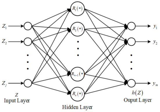
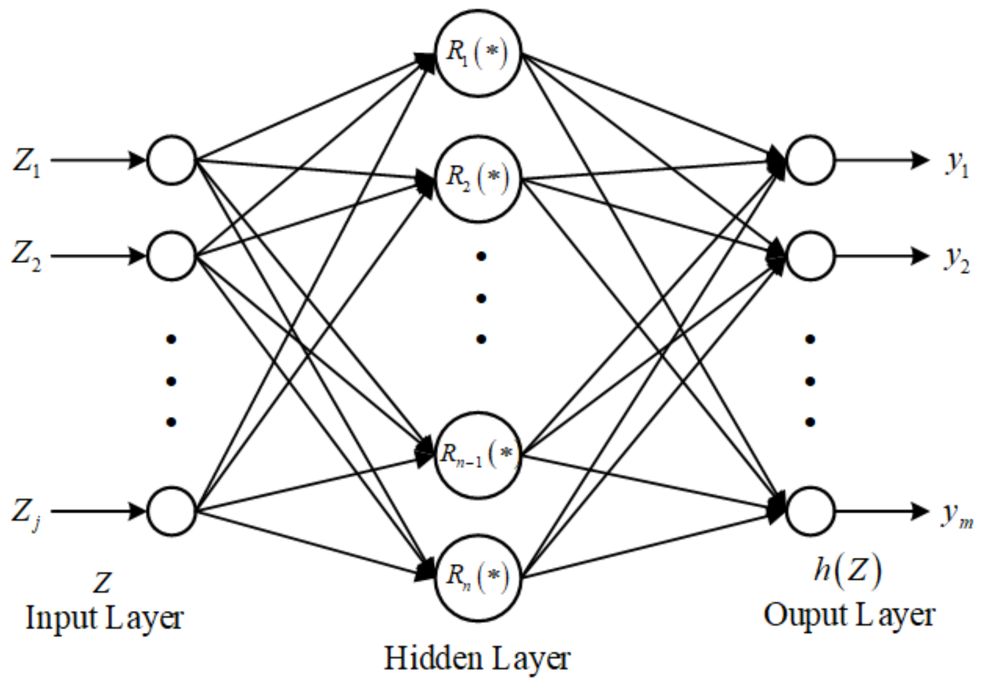
([35]). Let $h\left(Z\right)$ be an unknown continuous function over a compact set ${\mathsf{\Omega }}_Z\subset R^m$; for $\forall \overline{\delta }>0$ and with $m>0$ being the NN node number, there exists a radial basis function (RBF) NN, satisfying the following:

$$h\left(Z\right)={\varphi }^{T}R\left(Z\right)+\delta \left(Z\right),∥\delta \left(Z\right)∥\le \overline{\delta }$$

(8)

where

$${\varphi }^T=\arg {\min }_{\varphi \in R^n}\left\{\underset{Z\in {\mathsf{\Omega }}_Z}{sup}\left|h\left(Z\right)-{\varphi }^{T}R\left(Z\right)\right|\right\}$$

(9)

where $Z=\left[Z_1,\cdots ,Z_m\right]\in R^m$ denotes the input vector, $\varphi ={[{\varphi }_1,{\varphi }_2,\dots ,{\varphi }_m]}^T\subset R^m$ represents the ideal weight vectors. $\delta \left(x\right)$ indicates the approaching error, $R\left(Z\right)={[R_1\left(Z\right),\dots ,R_m\left(Z\right)]}^T$ represents the vectors of RBF basis functions, which can be shown as follows:

$$R_i\left(x\right)=exp\left[-\frac{{∥Z-c_{r_i}∥}^2}{{\sigma }_{NN,i}^2}\right]$$

(10)

in which $c_i={[c_{i1},c_{i2},\dots c_{im}]}^T$ and ${\sigma }_{NN,i}$ are the center and breadth of the RBF NN radial basis functions, respectively. The structure of NN used in this paper is depicted in Figure 1.

Figure 1. Neural network structure.

Lemma 6

([36]). The following inequality holds for any ${\sigma }_i\in R^{+}$ and for any $\varpi \in R$

$$\left|\varpi \right|-\frac{{\varpi }^2}{\sqrt{{\varpi }^2+{\epsilon }_i^2}}\le {\epsilon }_i$$

(11)

2.3. Practical Virtual Controller

Since the virtual control signals perform control operations in the system corresponding to the state variables, a practical virtual controller transformation is introduced in order to make them conform to the state constraints of the corresponding states. Using the concepts of the hyperbolic tangent function as well as the saturation function, a practical virtual controller transformation function is constructed as follows:

$$\varphi \left(\alpha \right)=Dtanh\left(\frac{\alpha }{D}\right)$$

(12)

where D represents the state constraint value for the corresponding state. The designed virtual controller is introduced to the conversion function and the system control task is replaced by the output practical virtual controller. The constraints on the virtual control signals can be realized by using the saturation property of the practical virtual controller function. Then, using the familiar differential median theorem, it is easy to see that at the point ${\alpha }^{\ast }$, and the constant $0<\mu <1$, there exists

$$\varphi \left(\alpha \right)={\left.\frac{\partial \varphi \left(\alpha \right)}{\partial \alpha }\right|}_{\alpha ={\alpha }_{\mu }}\left(\alpha -{\alpha }_0\right)+\varphi \left({\alpha }_0\right)$$

(13)

in which ${\alpha }_{\mu }=\mu \alpha +\left(1-\mu \right){\alpha }_0$. Let ${\alpha }_0=0$, one can obtain

$$\varphi \left(\alpha \right)={\varphi }_{\alpha }\alpha$$

(14)

where ${\varphi }_{\alpha }={\left.\frac{\partial \varphi \left(\alpha \right)}{\partial \alpha }\right|}_{\alpha ={\alpha }_{\mu }}$. Since the hyperbolic tangent function is monotonically increasing in the interval $\left(-\infty ,+\infty \right)$, it can be assumed—without loss of generality—that $0<b_i<{\varphi }_{\alpha }\le 1$, which will be used in each step of the controller design section.

2.4. System Description

Consider the following class of stochastic nonlinear systems:

$$\begin{array}{cc}\hfill & d{x}_i=(g_i\left(x_i\right)x_{i+1}\left(t\right)+f_i\left({\overline{x}}_i\right)dt+{\phi }_i\left(t\right)d\omega \hfill \\ \hfill & d{x}_n=(g_n\left(x_n\right)u\left(t\right)+f_n\left({\overline{x}}_n\right))dt+{\phi }_n\left(t\right)d\omega \hfill \\ \hfill & y\left(t\right)=x_1\left(t\right)\hfill \end{array}$$

(15)

where ${\overline{x}}_i\left(t\right)={[x_1\left(t\right),x_2\left(t\right),\dots ,x_i\left(t\right)]}^T\in R^i,i=1,\dots ,n$ signifies the state, $y\in R$ signifies the system output, $f_i\left(\blacksquare \right)$ and $g_i\left(\blacksquare \right)$ represent the smooth functions that are nonlinear. $u\left(t\right)$ denotes control inputs subject to nonlinearities of multiple actuator constraints, described as follows:

$$u=h\left(v\right)v+\pi \left(v\right)$$

(16)

where v represents the input signal for dead zone and saturation nonlinear models. Parameters $l_{+},l_{-},u_{+},u_{-}$ are design parameters, $u_H,u_L$ represent the positive normal numbers to be designed. $h\left(v\right),\pi \left(v\right)$ are described as follows:

$$h\left(v\right)=\left\{\begin{array}{cc}\hfill & \frac{u_H}{v},v>u_H\hfill \\ \hfill & l_{+},u_{+}<v<u_H\hfill \\ \hfill & 0,-u_{-}<v<u_{+}\hfill \\ \hfill & l_{-},-u_L<v<u_{-}\hfill \\ \hfill & -\frac{u_L}{v},v<-u_L\hfill \end{array}\right.$$

(17)

$$\pi \left(v\right)=\left\{\begin{array}{cc}\hfill & 0,v>u_H\hfill \\ \hfill & -l_{+}{u}_{+},u_{+}<v<u_H\hfill \\ \hfill & 0,-u_{-}<v<u_{+}\hfill \\ \hfill & -l_{-}{u}_{-},-u_L<v<u_{-}\hfill \\ \hfill & 0,v<-u_L\hfill \end{array}\right.$$

(18)

Assumption 1

([37]). Two slopes of the deadband and saturation nonlinear models are equal, i.e., $l_{+}=l_{-}=l$. Dead zone parameters of the controller $u_{+},u_{-}$ and l are bounded, i.e., the existence of known parameters $u_{+max},u_{-max}$ and $l_{max}$ that $\left|u_{+}\right|<u_{+max},\left|u_{-}\right|<u_{-max}$ and $\left|l\right|<l_{max}$.

Remark 3.

It is easy to conclude from Assumption 2 that $\left|\pi \left(v\right)\right|\le H$, where H represents the upper limit value; this feature can greatly reduce the controller design workload.

Assumption 2.

The anticipated tracking trace signals $y_d$ and their nth-order derivatives $y_d^{\left(n\right)}$ considered in this paper are continuous and bounded. Furthermore, to simplify the representation of the subsequent time-varying constraint functions, the following equations are listed, for constants $d_1$ and $d_2$

$$L_{y\left(t\right)}<d_1<y_d<d_2<H_{y\left(t\right)}$$

(19)

Assumption 3.

Functions $g_i\left(x_i\right)$ are bounded. Suppose that there are constants $a_i$, there exists $0<a_i\le \left|g_i\left(x_i\right)\right|<\infty ,i=1,2,\dots ,n$.

Remark 4.

Consider the actual situation; the control input v must be bounded. Then, consider that $m\left(v\right)$, the following inequality naturally holds:

$$0<r\le min\left\{\frac{u_H}{v_{max}},l\right\}\le h\left(v\right)\le max\left\{1,l\right\}$$

(20)

where $v_{max}$ represents the maximum value of the designed controller.

The control objective of this paper is to design an adaptive control strategy, such that (1) all variables of the controlled system are bounded; (2) all system states do not violate their constraint boundaries; (3) system inputs obey the limits of dead zone and saturation constraints; and (4) the virtual controllers that perform the control tasks satisfy the constraints of the corresponding system states. For the convenience of the proof, we set $g_i=g_i\left(x_i\right),f_i=f_i\left({\overline{x}}_i\right)$ and all the time variables t will be omitted in the following.

3. Adaptive NN Control Design and Stability Analysis

Building on the previous section, this section shows the detailed steps for designing a neural adaptive tracking controller using the backstepping method. In the first step, for a given reference trajectory signal $y_d\left(t\right)$, the system output tracking error is designed as $z_1=y-y_d$. In the next step, the virtual controller is designed as ${\alpha }_i$. In the control process, $\varphi \left(a_i\right)$, a new function defined by ${\alpha }_i$ will be specified later. During the controller design process, $\varphi \left(a_i\right)$ will replace ${\alpha }_i$ and completely substitute the control work of ${\alpha }_i$. To distinguish it from the original virtual controller, this is named the practical virtual controller. To realize the task with full state constraints, in step i, we design the practical virtual tracking error to be $z_i=x_i-\varphi \left({\alpha }_{i-1}\right)\left(1<i\le n\right)$. The GBLF method will be used to solve the state constraints task and, therefore, give the expression for the associated tracking error $z_i$ constraint as follows:

$$\left\{\begin{array}{cc}\hfill & -D_{L1}<z_1<D_{H1}\hfill \\ \hfill & -D_i<z_i<D_i\hfill \end{array}\right.$$

(21)

where $D_{L1},D_{H1}$ are in a time-varying function form and $D_i$ is in real-number form.

From system (15), we can obtain the dynamics of $z_1$, $z_i$, and $z_n$ as follows

$$d{z}_1=(g_1{x}_2+f_1-{\dot{y}}_d)dt+{\phi }_{1}d\omega$$

(22)

$$d{z}_i=(g_i{x}_{i+1}+f_i-\dot{\varphi }\left({\alpha }_{i-1}\right))dt+{\overline{\phi }}_{i}d\omega$$

(23)

$$d{z}_n=(g_{n}h\left(v\right)v+g_n\pi \left(v\right)+f_n-\dot{\varphi }\left({\alpha }_{n-1}\right))dt+{\overline{\phi }}_{n}d\omega$$

(24)

where ${\overline{\phi }}_i={\left({\phi }_i-{\displaystyle \sum _{i=1}^{i-1}}\frac{\partial \varphi \left(a_{i-1}\right)}{\partial {\xi }_j}{\phi }_j\right)}^T(i=2,\dots ,n)$,

$$\begin{array}{cc}\hfill & \dot{\varphi }\left({\alpha }_{i-1}\right)=\sum _{j=1}^{i-1}\frac{\partial \varphi \left({\alpha }_{i-1}\right)}{\partial x_j}\left[f_j+g_j{x}_{j+1}\right]+\sum _{j=1}^{i-1}\frac{\partial \varphi \left({\alpha }_{i-1}\right)}{\partial {\widehat{\theta }}_j}{\dot{\widehat{\theta }}}_j\hfill \\ \hfill & +\sum _{j=0}^{i-1}\frac{\partial \varphi \left({\alpha }_{i-1}\right)}{\partial y_d^{\left(j\right)}}{y}_d^{j+1}+\frac{1}{2}\sum _{p,q=1}^{i-1}\frac{{\partial }^2\varphi \left({\alpha }_{i-1}\right)}{\partial x_p\partial x_q}{\phi }_p^T{\phi }_q\hfill \end{array}$$

(25)

which $i=1,2,\dots ,n$.

Step 1: Construct the following GBLF

$$V_1=\frac{1}{4}{\xi }_1^4+\frac{{\gamma }_1}{2}{\tilde{\theta }}_1^2,{\xi }_1=\frac{D_{L1}{D}_{H1}{z}_1}{(D_{H1}-z_1)(D_{L1}+z_1)}$$

(26)

where ${\gamma }_1=a_1{b}_1$, ${\tilde{\theta }}_1={\theta }_1-{\widehat{\theta }}_1$, in which ${\widehat{\theta }}_1$ denotes the estimate of the uncertain parameter ${\theta }_1$. To simplify the arithmetic process, the coefficient terms are first defined as

$${\xi }_{\Delta }={\prod }_1{\dot{D}}_{H1}+{\prod }_2{\dot{D}}_{L1},{\Delta }_1=\frac{D_{H1}{D}_{L1}\left(D_{H1}{D}_{L1}+z_1^2\right)}{{\left(D_{H1}-z_1\right)}^2{\left(D_{L1}+z_1\right)}^2}$$

(27)

where ${\prod }_1=\frac{-D_{L1}{z}_1^2}{{\left(D_{H1}-z_1\right)}^2\left(D_{L1}+z_1\right)}$, ${\prod }_2=\frac{D_{H1}{z}_1^2}{\left(D_{H1}-z_1\right){\left(D_{L1}+z_1\right)}^2}$.

Taking the time derivative of $V_1$ yields

$$\begin{array}{cc}\hfill & L{V}_1={\xi }_1^3{\xi }_{\Delta }+{\xi }_1^3(f_1+g_1{x}_2-{\dot{y}}_d){\Delta }_1-{\gamma }_1{\tilde{\theta }}_1{\dot{\widehat{\theta }}}_1+\frac{3}{2}{\xi }_1^2{\phi }_1^T{\phi }_1\hfill \\ \hfill & ={\xi }_1^3{\Delta }_1(F_1\left(Z_1\right)+g_1\varphi \left({\alpha }_1\right))+{\xi }_1^3{\Delta }_1{g}_1{z}_2-\frac{3{\xi }_1^4}{4{\varsigma }_1^2}{∥{\phi }_1∥}^4-{\gamma }_1{\tilde{\theta }}_1{\dot{\widehat{\theta }}}_1+\frac{3}{2}{\xi }_1^2{\phi }_1^T{\phi }_1\hfill \end{array}$$

(28)

where $F_1\left(Z_1\right)=\frac{{\xi }_{\Delta }}{{\Delta }_1}+f_1-{\dot{y}}_d+\frac{3{\xi }_1}{4{\varsigma }_1^2{\Delta }_1}{∥{\phi }_1∥}^4$ and $Z_1={\left[x_1,y_d,{\dot{y}}_d,D_{H1},D_{L1},{\dot{D}}_{H1},{\dot{D}}_{L1}\right]}^T$. Based on the approximation ability of NNs as well as Lemma 5, as to any constant $\delta$, the following equality holds:

$$F_1\left(Z_1\right)={\varphi }_1^T{R}_1\left(Z_1\right)+{\delta }_1\left(Z_1\right)\left|{\delta }_1\left(Z_1\right)\right|\le \delta$$

(29)

According to Lemma 1, it follows that

$$\begin{array}{cc}\hfill & {\xi }_1^3{\Delta }_1({\varphi }_1^T{R}_1\left(Z_1\right)+{\delta }_1\left(Z_1\right))\hfill \\ \hfill & \le \left|{\xi }_1^3\right|{\Delta }_1(∥{\varphi }_1^T∥∥R_1\left(Z_1\right)∥+\left|{\delta }_1\left(Z_1\right)\right|)\hfill \\ \hfill & \le \left|{\xi }_1^3\right|{\Delta }_1{\gamma }_1{\theta }_1{\hslash }_1\hfill \\ \hfill & \le {\xi }_1^3{\Delta }_1{\gamma }_1{\theta }_1{\hslash }_{1}tanh(\frac{{\xi }_1^3{\Delta }_1{\hslash }_1}{{\tau }_1})+\varsigma {\tau }_1{\gamma }_1{\theta }_1\hfill \end{array}$$

(30)

where $\theta =([max\{{\delta }_1,∥{\varphi }_1^T∥\}/{\gamma }_1])$ and ${\hslash }_1=(1+∥R_1\left(Z_1\right)∥)$.

According to Young’s inequality, the following inequality holds

$$\frac{3}{2}{\xi }_1^2{\phi }_1^T{\phi }_1\le \frac{3}{4{\varsigma }_1^2}{\xi }_1^4{∥{\phi }_1∥}^4+\frac{3}{4}{\varsigma }_1^2$$

(31)

where ${\varsigma }_1>0$ denotes design parameters. With the aid of (28) (30), we can obtain

$$\begin{array}{cc}\hfill & L{V}_1\le {\xi }_1^3{\Delta }_1{g}_1\varphi \left({\alpha }_1\right)+{\xi }_1^3{\Delta }_1{g}_1{z}_2-{\gamma }_1{\tilde{\theta }}_1{\dot{\widehat{\theta }}}_1\hfill \\ \hfill & +{\xi }_1^3{\Delta }_1{\gamma }_1{\theta }_1{\hslash }_{1}tanh(\frac{{\xi }_1^3{\Delta }_1{\hslash }_1}{{\tau }_1})+\varsigma {\tau }_1{\gamma }_1{\theta }_1+\frac{3}{4}{\varsigma }_1^2\hfill \end{array}$$

(32)

We construct virtual control laws and adaptive laws as follows:

$${\alpha }_1=-\frac{1}{{\Delta }_1{\gamma }_1}\frac{{\xi }_1{\overline{\alpha }}_1^2}{\sqrt{{\xi }_1^4{\overline{\alpha }}_1^2+{\epsilon }_1^2}}$$

(33)

$${\overline{\alpha }}_1=k_{11}{(\frac{1}{4})}^{\frac{3}{4}}{\xi }_1+k_{12}{\left(\frac{1}{4}\right)}^2{\xi }_1^6+{\xi }_1{\gamma }_1{\widehat{\theta }}_1{\Delta }_1{\hslash }_{1}tanh(\frac{{\xi }_1^3{\Delta }_1{\hslash }_1}{{\tau }_1})$$

(34)

$${\dot{\widehat{\theta }}}_1={\xi }_1^3{\Delta }_1{\hslash }_{1}tanh(\frac{{\xi }_1^3{\Delta }_1{\hslash }_1}{{\tau }_1})-\frac{{\eta }_1}{{\gamma }_1}{\widehat{\theta }}_1-\frac{{\kappa }_1}{{\gamma }_1}{\widehat{\theta }}_1^3$$

(35)

According to Lemma 6, it follows that

$$\begin{array}{cc}\hfill & {\xi }_1^3{\Delta }_1{g}_1\varphi \left({\alpha }_1\right)={\xi }_1^3{\Delta }_1{g}_1{\varphi }_{{\alpha }_1}{\alpha }_1\hfill \\ \hfill & \le {\epsilon }_1-{\xi }_1^2{\overline{\alpha }}_1\hfill \end{array}$$

(36)

Substituting (33)–(36) into (32), yields

$$L{V}_1\le -k_{11}{(\frac{{\xi }_1^4}{4})}^{\frac{3}{4}}-k_{12}{(\frac{{\xi }_1^4}{4})}^2+{\xi }_1^3{\Delta }_1{g}_1{z}_2+{\eta }_1{\tilde{\theta }}_1{\widehat{\theta }}_1+{\kappa }_1{\tilde{\theta }}_1{\widehat{\theta }}_1^3+{\sigma }_1$$

(37)

where ${\sigma }_1={\epsilon }_1+\frac{3}{4}{\varsigma }_1^2+\varsigma {\tau }_1{\gamma }_1{\theta }_1$.

Step i: Construct the following GBLF

$$V_i=\frac{1}{4}{\xi }_i^4+\frac{{\gamma }_i}{2}{\tilde{\theta }}_i^2,{\xi }_i=\frac{D_i^2{z}_i}{D_i^2-z_i^2}$$

(38)

where ${\gamma }_i=a_i{b}_i$, ${\tilde{\theta }}_i={\theta }_i-{\widehat{\theta }}_i$, in which ${\widehat{\theta }}_i$ represents the estimated value of ${\theta }_i$.

To simplify the arithmetic process, we define the coefficient terms and the additional terms as

$${\Delta }_i=\frac{D_i^2\left(D_i^2+z_i^2\right)}{{\left(D_i^2-z_i^2\right)}^2},\left(i=2,\dots ,n\right)$$

(39)

$${\mathsf{\Psi }}_i={\xi }_{i-1}^3{\Delta }_{i-1}{g}_{i-1}{z}_i,\left(i=2,3,\dots n\right)$$

(40)

Taking the time derivative of $V_i$ yields

$$\begin{array}{cc}\hfill & L{V}_i={\xi }_i^3(f_i+g_i{x}_{i+1}-\dot{\varphi }\left({\alpha }_{i-1}\right)){\Delta }_i-{\gamma }_i{\tilde{\theta }}_i{\dot{\widehat{\theta }}}_i+\frac{3}{2}{\xi }_i^2{\overline{\phi }}_i^T{\overline{\phi }}_i\hfill \\ \hfill & ={\xi }_i^2{\Delta }_i{F}_i\left(Z_i\right)+{\xi }_i^3{\Delta }_i{g}_i\varphi \left({\alpha }_i\right)+{\xi }_i^3{\Delta }_i{g}_i{z}_{i+1}-\frac{3{\xi }_i^4}{4{\varsigma }_i^2}{∥{\overline{\phi }}_i∥}^4\hfill \\ \hfill & -{\gamma }_i{\tilde{\theta }}_i{\dot{\widehat{\theta }}}_i+\frac{3}{2}{\xi }_i^2{\overline{\phi }}_i^T{\overline{\phi }}_i-\frac{{\left({\mathsf{\Psi }}_i\right)}^2}{\sqrt{{\left({\mathsf{\Psi }}_i\right)}^2+{\epsilon }_i^2}}\hfill \end{array}$$

(41)

where $F_i\left(Z_i\right)={\xi }_i{f}_i-{\xi }_i\dot{\varphi }\left(v_{i-1}\right)+\frac{3{\xi }_i^2}{4{\varsigma }_i^2{\Delta }_i}{∥{\overline{\phi }}_i∥}^4+\frac{{\left({\xi }_{i-1}{\Delta }_{i-1}{g}_{i-1}\right)}^2(D_i^2+z_i^2)}{{\Delta }_i^2{D}_i^2\sqrt{{\mathsf{\Psi }}_i^2+{\epsilon }_i^2}}$. Based on the approximation ability of NNs as well as Lemma 5, as to any constant $\delta$, the following equality holds:

$$F_i\left(Z_i\right)={\varphi }_i^T{R}_i\left(Z_i\right)+{\delta }_i\left(Z_i\right),\left|{\delta }_i\left(Z_i\right)\right|\le \delta$$

(42)

According to Lemma 1, it follows that

$$\begin{array}{cc}\hfill & {\xi }_i^2{\Delta }_i({\varphi }_i^T{R}_i\left(Z_i\right)+{\delta }_i\left(Z_i\right))\hfill \\ \hfill & \le {\xi }_i^2{\Delta }_i{\gamma }_i{\theta }_i{\hslash }_{i}tanh(\frac{{\xi }_i^2{\Delta }_i{\hslash }_i}{{\tau }_i})+\varsigma {\tau }_i{\gamma }_i{\theta }_i\hfill \end{array}$$

(43)

where ${\theta }_i=([max\{{\delta }_i,∥{\varphi }_i^T∥\}/{\gamma }_i])$ and ${\hslash }_1=(1+∥R_1\left(Z_1\right)∥)$. According to Young’s inequality, the following inequality holds

$$\frac{3}{2}{\xi }_i^2{\overline{\phi }}_i^T{\overline{\phi }}_i\le \frac{3}{4{\varsigma }_i^2}{\xi }_i^4{\overline{\phi }}_i^4+\frac{3}{4}{\varsigma }_i^2$$

(44)

Construct virtual control laws and adaptive laws as

$${\alpha }_i=-\frac{1}{{\Delta }_i{\gamma }_i}\frac{{\xi }_i{\overline{\alpha }}_i^2}{\sqrt{{\xi }_i^4{\overline{\alpha }}_i^2+{\epsilon }_i^2}}$$

(45)

$${\overline{\alpha }}_i=k_{i1}{(\frac{1}{4})}^{\frac{3}{4}}{\xi }_i+k_{i2}{\left(\frac{1}{4}\right)}^2{\xi }_i^6+{\gamma }_i{\widehat{\theta }}_i{\Delta }_i{\hslash }_{i}tanh(\frac{{\xi }_i^2{\Delta }_i{\hslash }_i}{{\tau }_i})$$

(46)

$${\dot{\widehat{\theta }}}_i={\xi }_i^2{\Delta }_i{\hslash }_{i}tanh(\frac{{\xi }_i^2{\Delta }_i{\hslash }_i}{{\tau }_i})-\frac{{\eta }_i}{{\gamma }_i}{\widehat{\theta }}_i-\frac{{\kappa }_i}{{\gamma }_i}{\widehat{\theta }}_i^3$$

(47)

According to Lemma 6, it follows that

$$\begin{array}{cc}\hfill & {\xi }_i^3{\Delta }_i{g}_i\varphi \left({\alpha }_i\right)={\xi }_i^3{\Delta }_i{g}_i{\varphi }_{{\alpha }_i}{\alpha }_i\hfill \\ \hfill & \le {\epsilon }_i-{\xi }_i^2{\overline{\alpha }}_i\hfill \end{array}$$

(48)

Substituting (43)–(48) into (41), yields

$$L{V}_i\le -k_{i1}{(\frac{{\xi }_i^4}{4})}^{\frac{3}{4}}-k_{i2}{(\frac{{\xi }_i^4}{4})}^2+{\xi }_i^3{\Delta }_i{g}_i{z}_{i+1}+{\eta }_i{\tilde{\theta }}_i{\widehat{\theta }}_i+{\kappa }_i{\tilde{\theta }}_i{\widehat{\theta }}_i^3-\frac{{\left({\mathsf{\Psi }}_i\right)}^2}{\sqrt{{\left({\mathsf{\Psi }}_i\right)}^2+{\epsilon }_i^2}}+{\sigma }_i$$

(49)

where ${\sigma }_i={\epsilon }_i+\frac{3}{4}{\varsigma }_i^2+\varsigma {\tau }_i{\gamma }_i{\theta }_i$.

Step n: Construct the following GBLF

$$V_n=\frac{1}{4}{\xi }_n^4+\frac{{\gamma }_n}{2}{\tilde{\theta }}_n^2,{\xi }_n=\frac{D_n^2{z}_n}{D_n^2-z_n^2}$$

(50)

where ${\gamma }_n=a_n{b}_n$, ${\tilde{\theta }}_n={\theta }_n-{\widehat{\theta }}_n$, where ${\widehat{\theta }}_n$ represents the estimated value of ${\theta }_n$.

Taking the time derivative of $V_n$ gives

$$\begin{array}{cc}\hfill & L{V}_n={\xi }_n^3(f_n+g_{n}h\left(v\right)v+g_n\pi \left(v\right)-\dot{\varphi }\left({\alpha }_{n-1}\right)){\Delta }_n-{\gamma }_n{\tilde{\theta }}_n{\dot{\widehat{\theta }}}_n+\frac{3}{2}{\xi }_n^2{\overline{\phi }}_n^T{\overline{\phi }}_n\hfill \\ \hfill & \le {\xi }_n^2{\Delta }_n{F}_n\left(Z_n\right)+{\xi }_n^3{\Delta }_n{g}_{n}h\left(v\right)v-\frac{3{\xi }_n^4}{4{\varsigma }_n^2}{∥{\overline{\phi }}_n∥}^4-{\gamma }_n{\tilde{\theta }}_n{\dot{\widehat{\theta }}}_n+\frac{3}{2}{\xi }_n^2{\overline{\phi }}_n^T{\overline{\phi }}_n-\frac{{\left({\mathsf{\Psi }}_n\right)}^2}{\sqrt{{\left({\mathsf{\Psi }}_n\right)}^2+{\epsilon }_n^2}}\hfill \end{array}$$

(51)

where $F_n\left(Z_n\right)={\xi }_n{f}_n-{\xi }_n\dot{\varphi }\left(v_{n-1}\right)+{\xi }_{n}H{g}_n+\frac{3{\xi }_n^2}{4{\varsigma }_n^2{\Delta }_n}{∥{\overline{\phi }}_n∥}^4+\frac{{\left({\xi }_{n-1}{\Delta }_{n-1}{g}_{n-1}\right)}^2(D_n^2+z_n^2)}{{\Delta }_n^2{D}_n^2\sqrt{{\mathsf{\Psi }}_n^2+{\epsilon }_n^2}}$.

Construct the real control laws and adaptive laws as follows:

$$u=-\frac{1}{{\Delta }_n{a}_{n}r}\frac{{\xi }_n{\overline{\alpha }}_n^2}{\sqrt{{\xi }_n^4{\overline{\alpha }}_n^2+{\epsilon }_n^2}}$$

(52)

$${\overline{\alpha }}_n=k_{n1}{(\frac{1}{4})}^{\frac{3}{4}}{\xi }_n+k_{n2}{\left(\frac{1}{4}\right)}^2{\xi }_n^6+{\gamma }_n{\widehat{\theta }}_n{\Delta }_n{\hslash }_{n}tanh(\frac{{\xi }_n^2{\Delta }_n{\hslash }_n}{{\tau }_n})$$

(53)

$${\dot{\widehat{\theta }}}_n={\xi }_n^2{\Delta }_n{\hslash }_{n}tanh(\frac{{\xi }_n^2{\Delta }_n{\hslash }_n}{{\tau }_n})-\frac{{\eta }_n}{{\gamma }_n}{\widehat{\theta }}_n-\frac{{\kappa }_n}{{\gamma }_n}{\widehat{\theta }}_n^3$$

(54)

Similar to the n-1 steps above, it can be obtained that

$$L{V}_n\le -k_{n1}{(\frac{{\xi }_n^4}{4})}^{\frac{3}{4}}-k_{n2}{(\frac{{\xi }_n^4}{4})}^2+{\eta }_n{\tilde{\theta }}_n{\widehat{\theta }}_n+{\kappa }_n{\tilde{\theta }}_n{\widehat{\theta }}_n^3+{\sigma }_n-\frac{{\left({\mathsf{\Psi }}_n\right)}^2}{\sqrt{{\left({\mathsf{\Psi }}_n\right)}^2+{\epsilon }_n^2}}$$

(55)

where ${\sigma }_n={\epsilon }_n+\frac{3}{4}{G}_n^2+\varsigma {\tau }_n{\gamma }_n{\theta }_n$.

After the above discussion, the following theorem can be concluded.

Theorem 1.

For the stochastic nonlinear system (15) under Assumptions 1–3, we conclude that if the control input and the adaptive laws are selected as (33), (35), (45), (47), (52) and (54), then the controlled system is SGFSP and the system signal is almost certainly bounded.

The proof is presented in Appendix A.

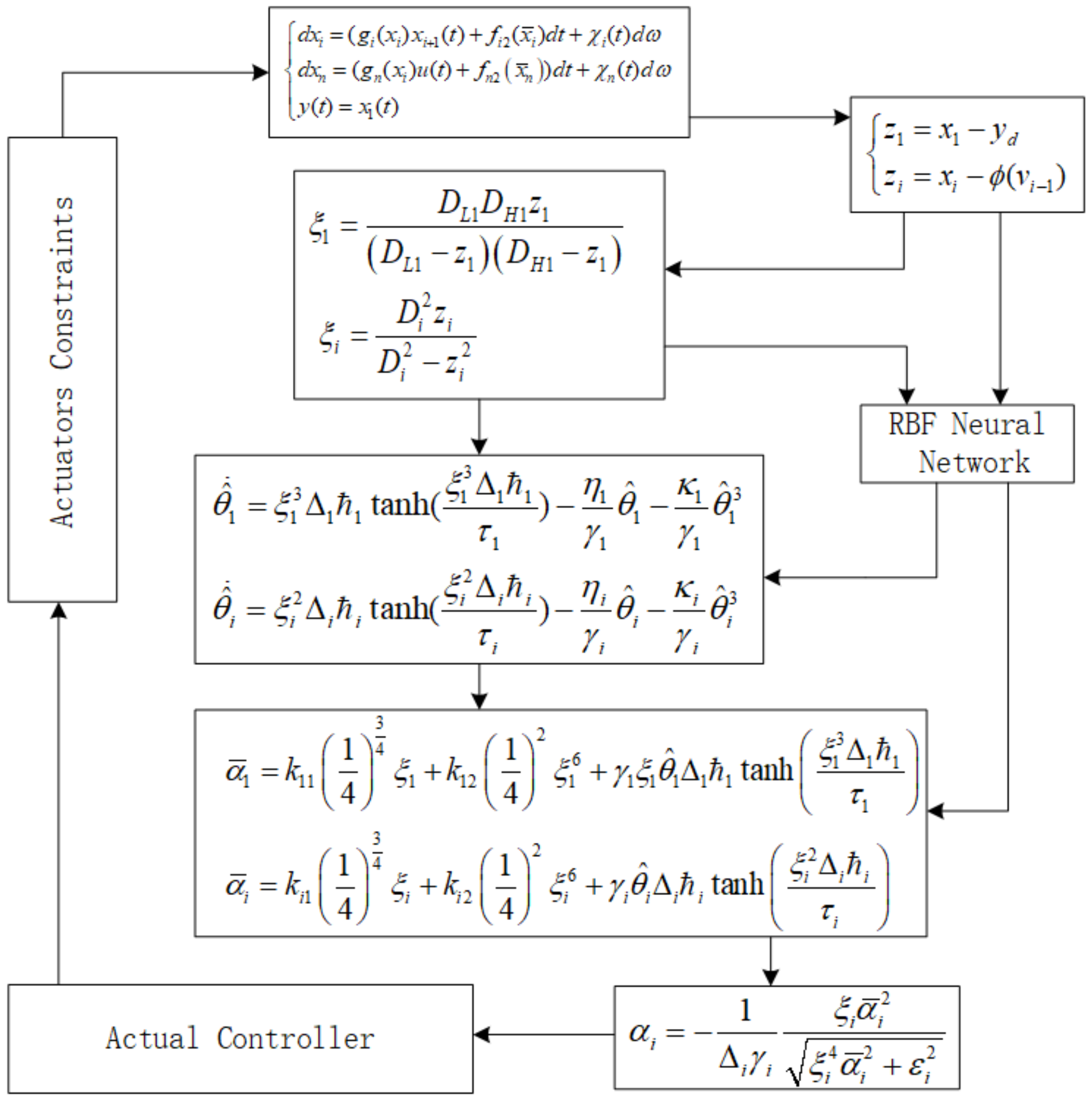
To obtain a clearer picture of the controller designed in this paper and to facilitate the design of the simulation in the next section, the adaptive NN control algorithm scheme is shown in Figure 2.

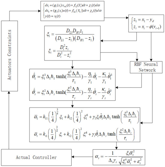
Figure 2. The block diagram of the control scheme.

4. Simulation

In the above formulation of the paper, the research work presented has been completed. In this section, two simulation examples will be used to verify the effectiveness of the proposed control strategy.

A. Mathematical example

The following second-order stochastic nonlinear system is used as the simulation object:

$$\begin{array}{cc}\hfill & {\dot{x}}_1=(x_2+e^{-0.5x_1^2})dt+0.5x_{1}d\omega \hfill \\ \hfill & {\dot{x}}_2=(x_{1}sin\left(x_2^2\right)+u)dt+0.5x_{1}d\omega \hfill \end{array}$$

(56)

where $x_i(i=1,2)$ is the state, $\mathrm{y}=x_1$ is the system output, and u represents the input to the system suffering from dead zone and saturation constraints. The control objective is to enable the system output to track the desired trajectory signal stably. Let the reference trajectory be $y_d=sin\left(t\right)$.

In order to construct a neural network-based adaptive controller, a set of nine neural networks is defined for each state variable on the interval $\left[-4,4\right]$ with the center point as $-4,-3,-2,-1,0,1,2,3,4$. The neural network basis vector function is $R_i\left(Z_i\right)={\left[R_i^1,R_i^2,\dots ,R_i^9\right]}^T$. The neural membership functions are defined by $R_i^l=exp\left(-0.5{\left(Z_i+\left(-5+l\right)\right)}^2\right)$ for $l=1,2,\dots 9$ and $Z_1={\left[x_1,y_d,{\dot{y}}_d,D_{H1},D_{L1},{\dot{D}}_{H1},{\dot{D}}_{L1}\right]}^T$, $Z_2={\left[x_1,x_2,{\xi }_1,{\xi }_2,{\widehat{\theta }}_1\right]}^T$.

The corresponding system state constraints and tracking error constraints as well as the system’s initial values and controller parameters are designed, as shown in Table 2. The relationship between the system input u and the design controller v, i.e., the dead zone and saturation nonlinear models, is described as follows:

$$u=\left\{\begin{array}{cc}\hfill & 52,v>52\hfill \\ \hfill & 0.7(v-0.6),0.6<v<52\hfill \\ \hfill & 0,-0.6<v<0.6\hfill \\ \hfill & 0.7(v+0.6),-20<v<-0.6\hfill \\ \hfill & -20,v<-20\hfill \end{array}\right.$$

(57)

Table 2. System parameters for A.

System Parameter
Constraint functions for system outputs and constraints for state $x_2$
$L_{y\left(t\right)}=sin\left(t\right)-0.2-0.4e^{-0.6t}$; $H_{y\left(t\right)}=sin\left(t\right)+0.3+0.4e^{-0.5t}$; $-3.41<x_2<3.41$
The constraint function or constraint value corresponding to the tracking error
$D_{L1}=0.2+0.4e^{-0.6t};D_{H1}=0.3+0.4e^{-0.6t}$; $D_2=\sqrt{2}$
Initial values and design parameters
${\left[x_1\left(0\right),x_2\left(0\right)\right]}^T={\left[0.5,-0.2\right]}^T$; ${\left[{\widehat{\theta }}_1\left(0\right),{\widehat{\theta }}_2\left(0\right)\right]}^T={\left[0.1,0.1\right]}^T$; $k_{11}=35,k_{12}=20$; $k_{21}=28,k_{22}=25$; $\gamma =2,{\tau }_1={\tau }_2=0.1$; ${\eta }_1={\eta }_2=2,k_1=k_2=1$; ${\epsilon }_1={\epsilon }_2=0.01$

In order to make the virtual controller also comply with the corresponding constraints, we design the following practical virtual control signals:

$$\varphi \left({\alpha }_1\right)=2tanh(\frac{{\alpha }_1}{2})$$

(58)

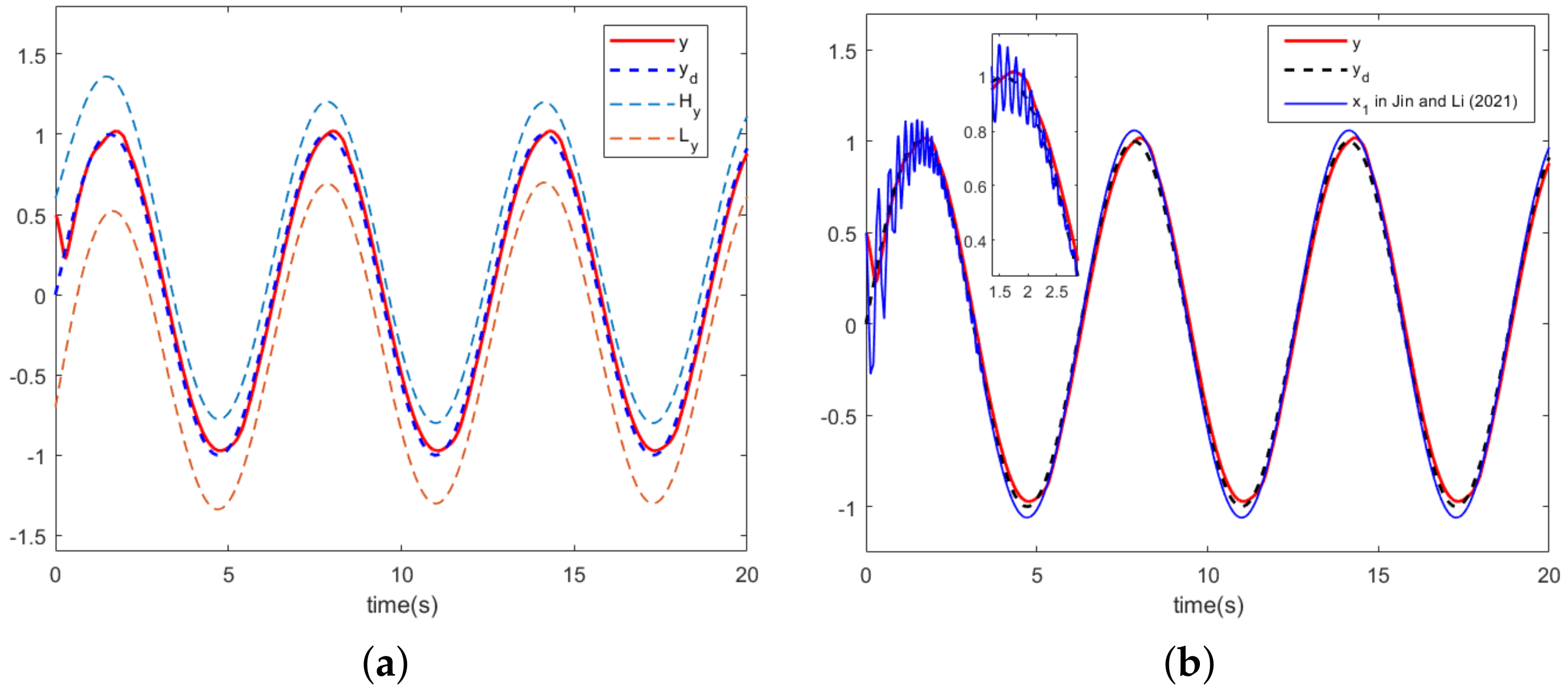
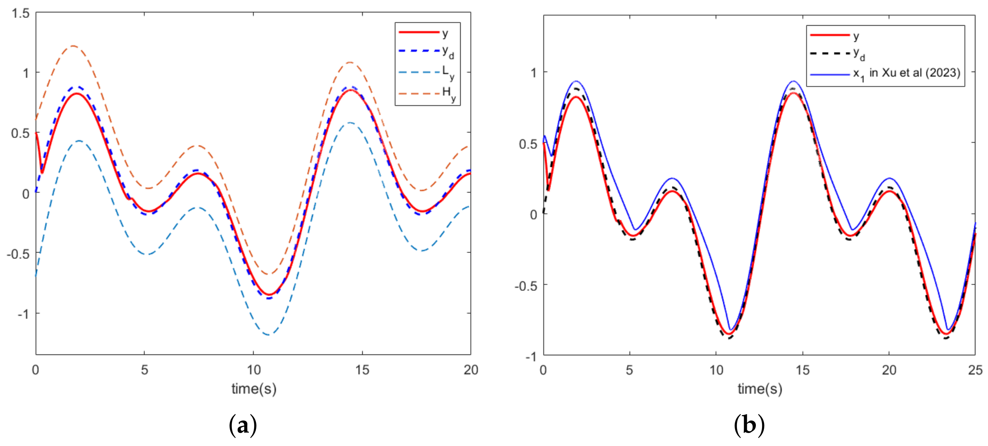
The simulation results in this example are presented in Figure 3, Figure 4, Figure 5, Figure 6 and Figure 7. Figure 3a depicts the trajectory of the system output, y, with the desired trajectory, yd. From Figure 3a, it can be seen that the control strategy designed in this paper has a good control performance, and the system output can quickly track the desired trajectory signals while satisfying the corresponding time-varying function constraints. The control scheme proposed in Reference [26], with the addition of the same dead zone and saturation constraint models used in this example, is compared with the scheme in this paper, and the trajectory comparison of the system output is shown in Figure 3b. From Figure 3b, it can be seen that the presence of dead zones and saturation constraints causes violent jitter in the early stage of the comparison control scheme, which demonstrates the effectiveness of the control strategy in this paper.

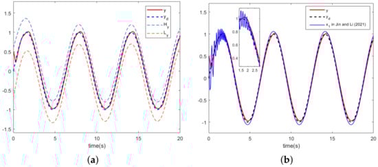
Figure 3. (a) System output and desired trajectory. (b) Output comparison with algorithms [26].

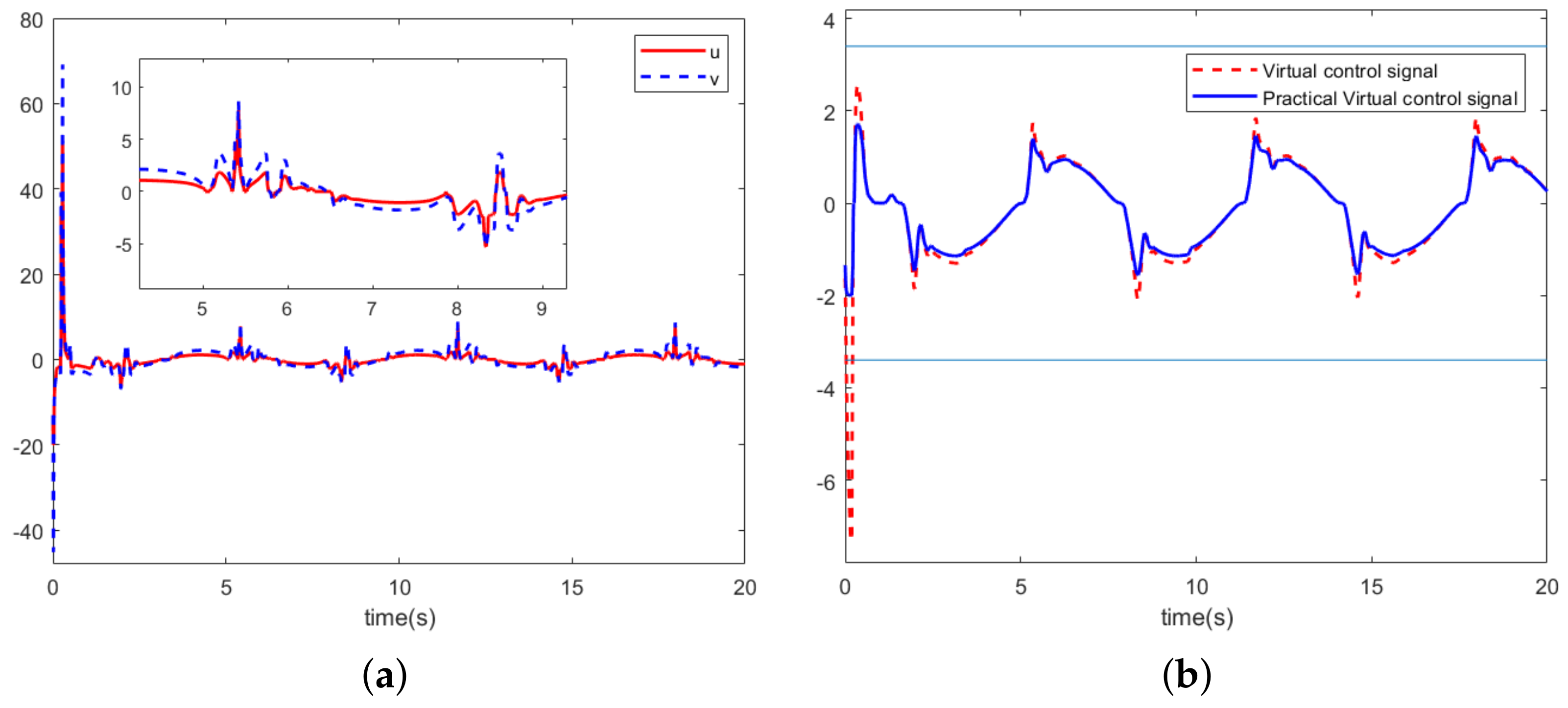
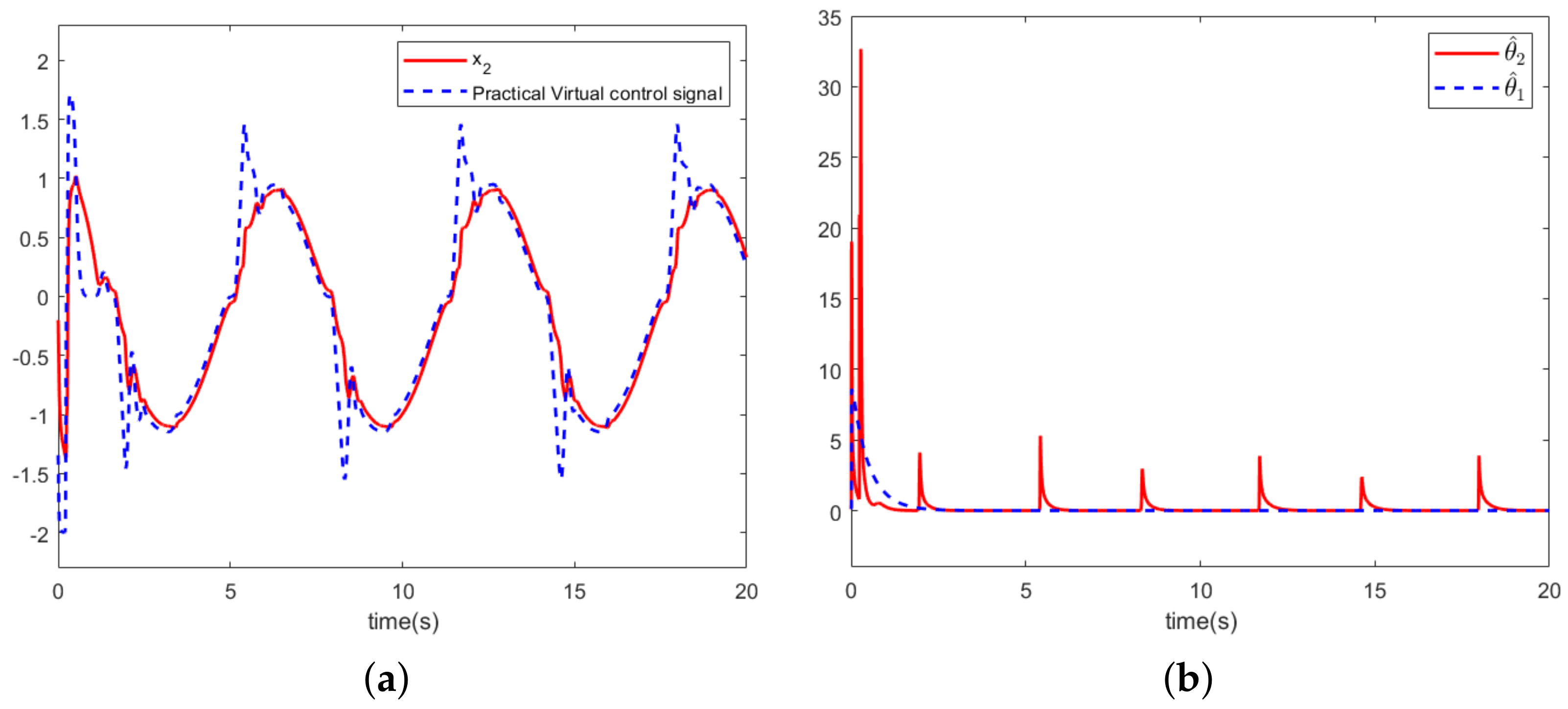
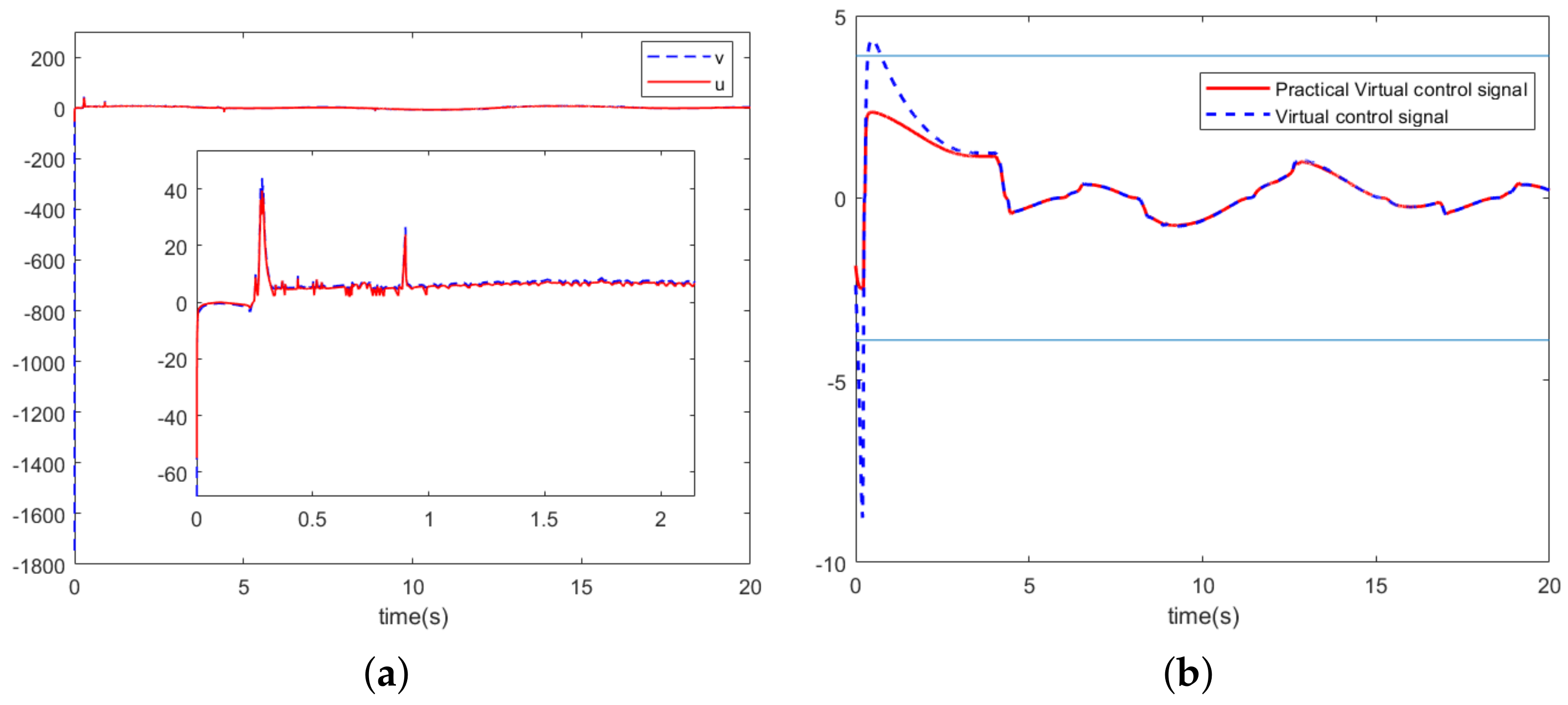
Figure 4. (a) Control input. (b) Virtual control signals.

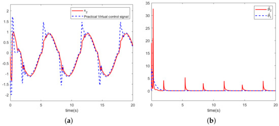
Figure 5. (a) State variable $x_2$. (b) Adaptive parameters.

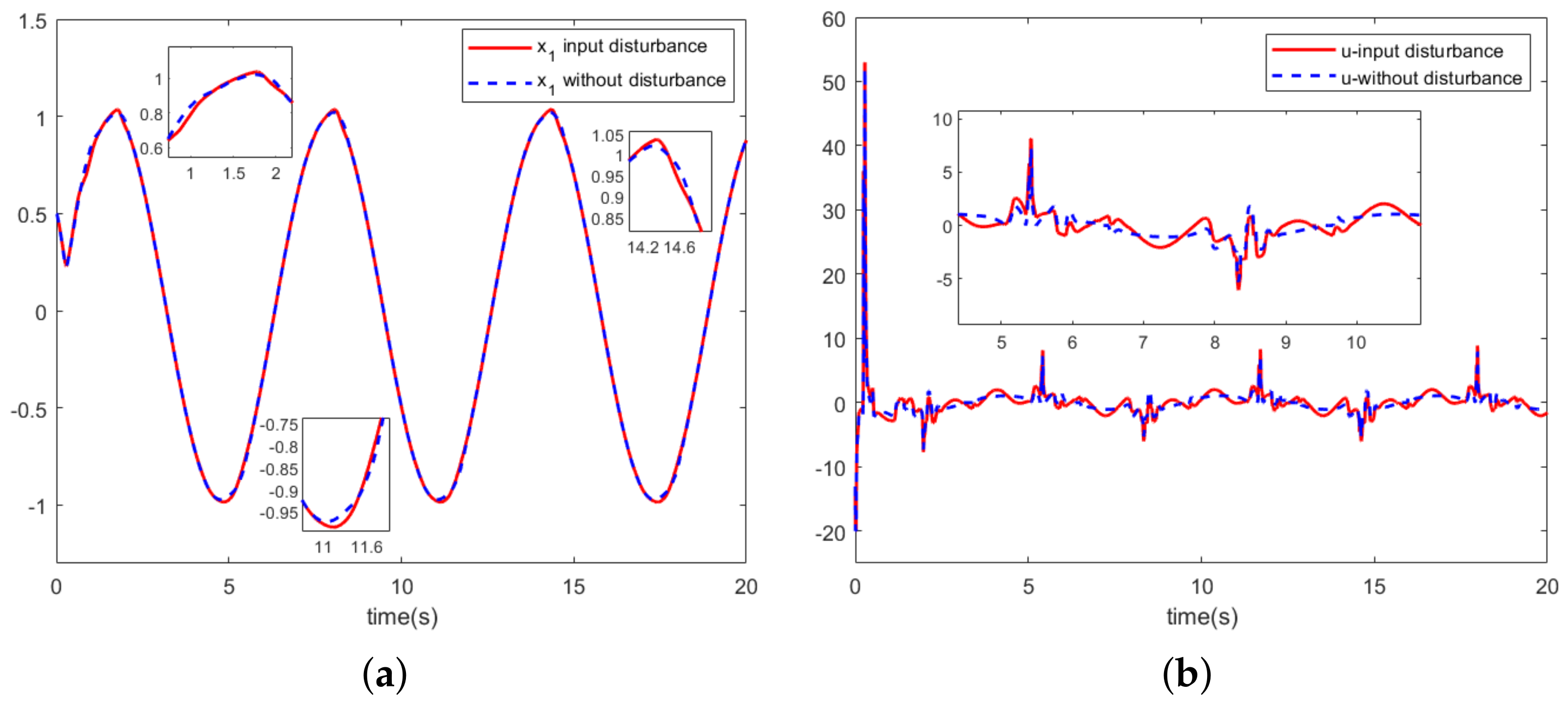
Figure 6. System output (a) and control input (b) with disturbance and without disturbance.

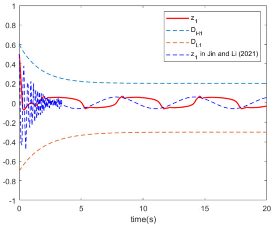
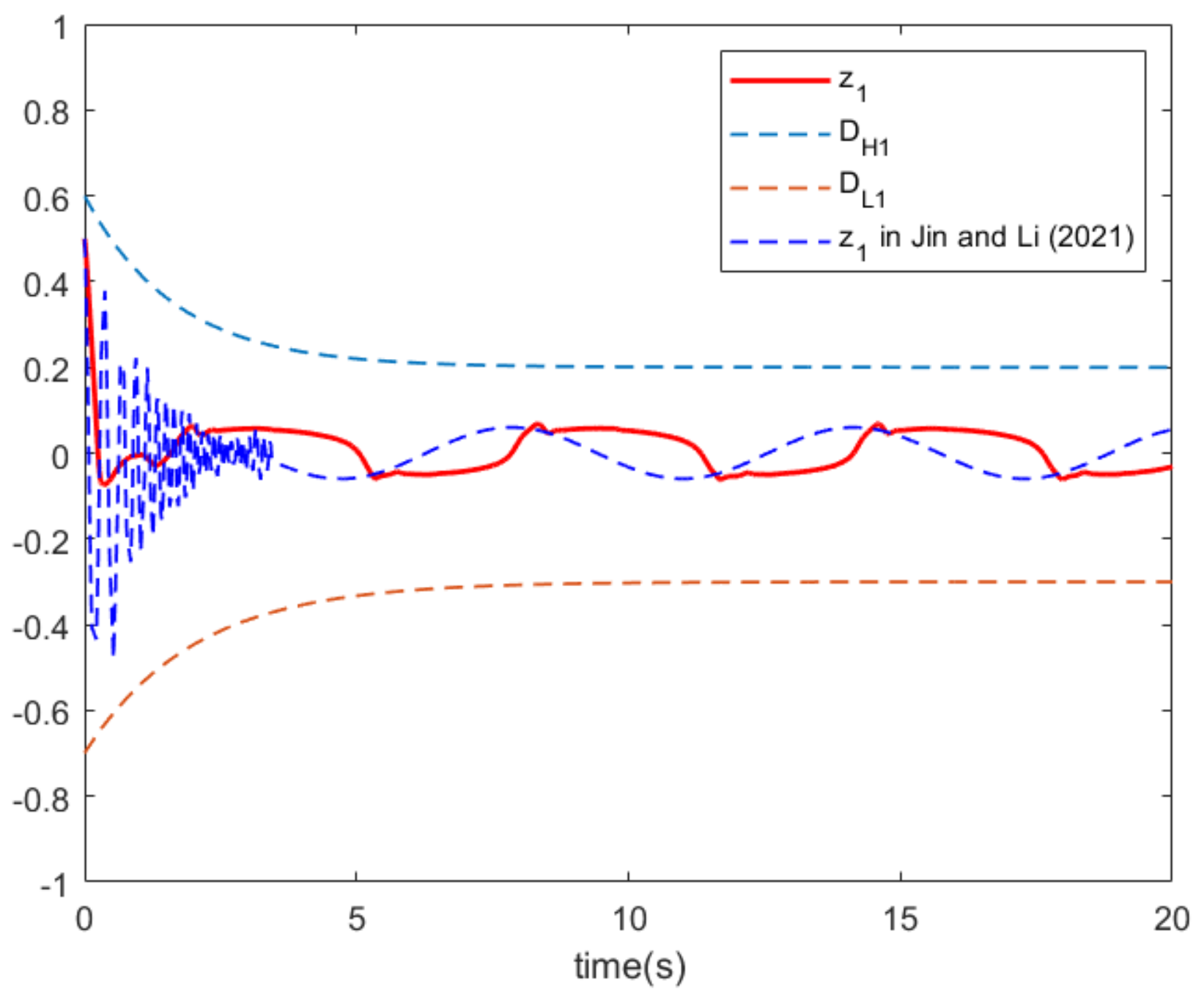
Figure 7. Tracking error of A and algorithms [26].

From the comparative simulation results, it can be seen that the control algorithm designed in this paper can cope with the tracking control of stochastic nonlinear systems with dead zones and saturated nonlinear constraints.

Figure 4a illustrates the controller trajectory and the control input trajectory suffering from dead zone and saturation nonlinearity constraints. Figure 4b illustrates the trajectory of the virtual control signal and the practical virtual controller. From Figure 4b, it can be seen that the practical virtual controller designed in this paper adheres to the constraints of the corresponding system states. The problem of $∥z_i∥=∥x_i∥-∥{\alpha }_{i-1}∥<L_i-∥{\alpha }_{i-1}∥=D_i<0$ is solved. Figure 5a,b illustrates the trajectory of the system state $x_2$ and adaptive parameters ${\widehat{\theta }}_1,{\widehat{\theta }}_2$. Figure 7 illustrates the output tracking error of the control strategy in this paper and the tracking error of the comparison scheme.

Remark 5.

In order to demonstrate the robustness and stability of the adaptive neural network tracking control algorithm proposed in this paper for stochastic nonlinear systems, we add perturbations $d\left(t\right)=1.2sin\left(5t\right)$ to the control input signal u. Figure 6a,b presents a comparison of the trajectories of the control input signal and the system output for additional disturbances and no disturbances. From the figure, it can be seen that the adaptive NN controller designed in this paper has good robustness and stability.

B. Simulations on a single-link manipulator system

A single-link manipulator system containing stochastic perturbations is used as an example to prove the practicality of the designed controller. The single-link manipulator system model is given as follows:

$$J\ddot{q}=-Mg{l}_{0}sin\left(q\right)-B\dot{q}+u\left(v\right)$$

(59)

where $q,\dot{q}$ and $\ddot{q}$ are the coordinate, velocity, and acceleration of angles, respectively. $u\left(v\right)$ is the input torque subject to saturation and deadband. Affected by white noise, the coefficient of viscous friction can be rewritten as $B=B_0+B_{\omega }\mathsf{\Theta }\left(t\right)$, where $\mathsf{\Theta }\left(t\right)$ satisfies ${\int }_0^t\mathsf{\Theta }\left(s\right)ds=\omega \left(t\right)$. Table 3 lists all the parameters of the single-link manipulator system.

Table 3. Example 2: Parameters of a single link robotic arm system.

Parameter	Description	Value
J	Torsion coefficient	0.5 kg·m2
M	Mess of the link	1 kg
g	Acceleration of gravity	9.8 m/s2
$l_0$	Length of the connecting rod	1 m
B	Coefficient of viscous friction	0.5 N·m·s
$B_{\omega }$	Noise coefficient	0.1 N·m·s

We can rewrite system (59) as follows:

$$\left\{\begin{array}{cc}\hfill & d{x}_1=x_{2}dt\hfill \\ \hfill & d{x}_2=2u\left(v\right)dt-\left(19.6sin\left(x_1\right)+x_2\right)dt-0.2x_{2}d\omega \hfill \\ \hfill & y=x_1\hfill \end{array}\right.$$

(60)

The corresponding system state constraints and tracking error constraints, as well as the system’s initial values and controller parameters, are designed as shown in Table 4. The practical virtual controller is designed as $\varphi \left({\alpha }_1\right)=2.5tanh({\alpha }_1/2.5)$. The relationship between the system input u and the design controller v, i.e., the dead zone and saturation nonlinear models, is described as follows:

$$u=\left\{\begin{array}{cc}\hfill & 50,v>50\hfill \\ \hfill & 0.6(v-0.6),0.6<v<50\hfill \\ \hfill & 0,-0.7<v<0.6\hfill \\ \hfill & 0.75(v+0.7),-55<v<-0.7\hfill \\ \hfill & -55,v<-55\hfill \end{array}\right.$$

(61)

Table 4. System parameters for B.

System Parameter
Constraint functions for system outputs and constraints for state $x_2$
$L_{y\left(t\right)}=0.5sin\left(t\right)+0.5sin\left(0.5t\right)-0.2-0.4e^{-0.6t}$; $H_{y\left(t\right)}=0.5sin\left(t\right)+0.5sin\left(0.5t\right)+0.3+0.4e^{-0.5t}$; $-3.91<x_2<3.91$
The constraint function or constraint value corresponding to the tracking error
$D_{L1}=0.2+0.4e^{-0.6t};D_{H1}=0.3+0.4e^{-0.6t}$; $D_2=\sqrt{2}$
Initial values and design parameters
${\left[x_1\left(0\right),x_2\left(0\right)\right]}^T={\left[0.5,0\right]}^T$; ${\left[{\widehat{\theta }}_1\left(0\right),{\widehat{\theta }}_2\left(0\right)\right]}^T={\left[1,0.5\right]}^T$; $k_{11}=28,k_{12}=25$, $k_{21}=25,k_{22}=20$; $\gamma =2,{\tau }_1={\tau }_2=0.1$; ${\eta }_1={\eta }_2=2,k_1=k_2=1$; ${\epsilon }_1={\epsilon }_2=0.01$

The simulation results in this section are presented in Figure 8, Figure 9 and Figure 10. Figure 8a depicts the trajectory of the system output y, the expectation trajectory $y_d$. The practical virtual controller of this paper is introduced to the scheme proposed in Reference [27] and then compared with the scheme designed in this paper, as shown in Figure 8b. As can be seen in Figure 8b, the tracking accuracy of the comparison schemes becomes significantly worse when the virtual controller satisfies the corresponding state constraints.

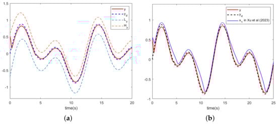
Figure 8. B. (a) System output. (b) Output comparison with algorithms [27].

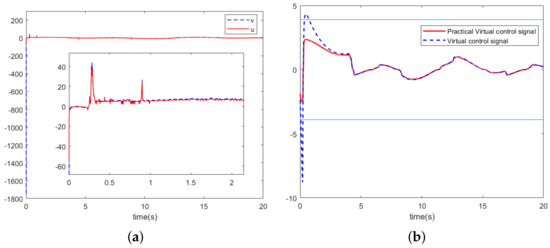
Figure 9. B. (a) Control input. (b) virtual control signals.

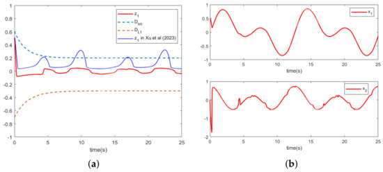
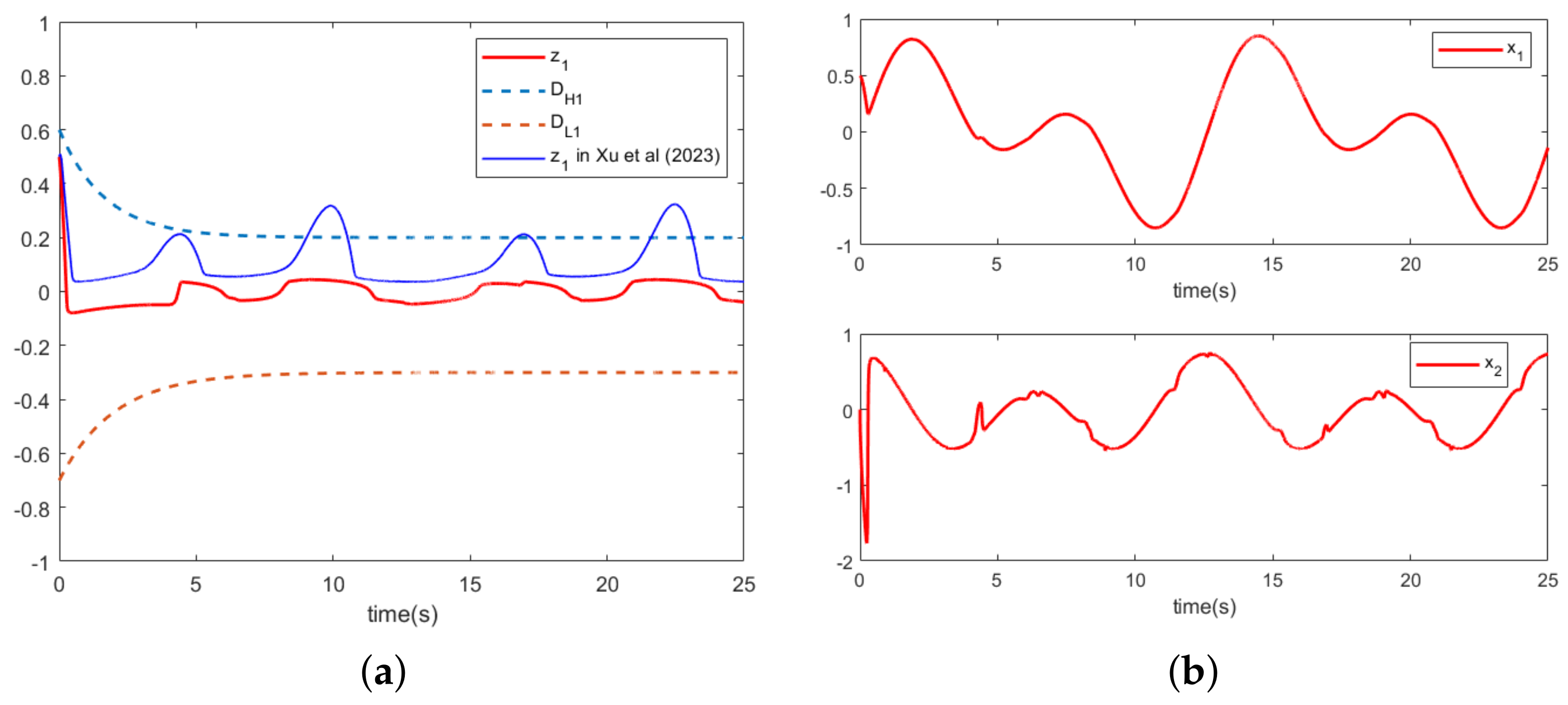
Figure 10. B. (a) Tracking error of B and algorithms [27]. (b) Trajectories of the system state.

By using practical virtual controllers instead of the original virtual control signals, all the signals performing control operations in the system control are in accordance with the corresponding constraints, which really achieves the full-state constraint control of stochastic nonlinear systems. As is well known, many practical physical systems such as flight vehicles, chemical reactors, and aircraft controls are subject to constraints to ensure the safe operation of the system. Therefore, as a control variable that performs the control task, imposing appropriate boundary constraints on the virtual control signal is also of considerable significance for the safe and reliable operation of the controlled system.

From Figure 9b, it can be seen that the practical virtual controller overcomes the issue of the original virtual controller violating the state constraints. Figure 10a demonstrates the system output tracking error for the control strategy of this paper and the comparison scheme. Figure 10 illustrates the trajectory of system states $x_1$, $x_2$.

Remark 6.

It is clear from Figure 9a that the original control input signal amplitude exceeds 1700, which is unlikely for a robotic arm system. After constraining by saturation and deadband, the control input signal amplitude is reduced to the achievable range without affecting the control performance.

From the simulation results shown in this section, it is easy to see that by applying the fixed-time neural network tracking controller designed in this paper and choosing the appropriate parameters, the system can obtain good tracking performance when all signals are bounded and the actual control inputs satisfy the dead zone and saturation constraints. In addition, the introduced practical virtual controller satisfies the constraints of the corresponding system states, and the control objective is achieved with all states and control variables in the system complying with the constraints, which proves the effectiveness and practicality of the designed control strategy.

5. Conclusions and Future Work

Since the uncertainty factor of randomness is often seen in practical application scenarios, in this paper, an adaptive neural network tracking control algorithm is designed for a class of stochastic nonlinear systems. It applies neural network approximation methods to address the interference of system uncertainty in controller design.

In order to practically meet the practical scenarios, this paper considers the full state constraints of the system. Compared with the existing fixed output constraints, the system output considered in this paper satisfies the time-varying function constraints, which have more practical relevance. With the corresponding actuator constraints, the actual control inputs can meet the demands of a realistic industrial production environment.

The use of practical virtual controllers ensures that the virtual control signals performing the control tasks always satisfy the constraints of the corresponding virtual control states throughout the control operation. The adaptive tracking control algorithm designed in this paper ensures that all the variables in the controlled system performing control tasks conform to the predefined boundary constraints; this is of great significance for the safe and reliable operation of real physical systems. Finally, the simulation demonstrates the control effect and verifies the effectiveness of the algorithm designed in this paper. In future research, adaptive fixed-time fault-tolerant control for MIMO stochastic nonlinear systems with full-state constraints will be considered.

References

- Imran, I.H.; Stolkin, R.; Montazeri, A. Adaptive Control of Quadrotor Unmanned Aerial Vehicle with Time-Varying Uncertainties. IEEE Access 2023, 11, 19710–19724. [Google Scholar] [CrossRef]
- Li, Z.; Chen, X.; Xie, M.; Zhao, Z. Adaptive fault-tolerant tracking control of flying-wing unmanned aerial vehicle with system input saturation and state constraints. Trans. Inst. Meas. Control. 2022, 44, 880–891. [Google Scholar] [CrossRef]
- Zhang, X.; Zhuang, Y.; Zhang, X.; Fang, Y. A Novel Asymptotic Robust Tracking Control Strategy for Rotorcraft UAVs. IEEE Trans. Autom. Sci. Eng. 2023, 20, 2338–2349. [Google Scholar] [CrossRef]
- Ba, D.; Li, Y.X.; Tong, S. Fixed-time adaptive neural tracking control for a class of uncertain nonstrict nonlinear systems. Neurocomputing 2019, 363, 273–280. [Google Scholar] [CrossRef]
- Sun, H.; Tu, L.; Yang, L.; Zhu, Z.; Zhen, S.; Chen, Y.H. Adaptive Robust Control for Nonlinear Mechanical Systems with Inequality Constraints and Uncertainties. IEEE Trans. Syst. Man Cybern. Syst. 2023, 53, 1761–1772. [Google Scholar] [CrossRef]
- Li, Y.; Zhu, Q.; Zhang, J. Distributed adaptive fixed-time neural networks control for nonaffine nonlinear multiagent systems. Sci. Rep. 2022, 12, 8459. [Google Scholar] [CrossRef]
- Zhao, K.; Chen, L.; Meng, W.; Zhao, L. Unified Mapping Function-Based Neuroadaptive Control of Constrained Uncertain Robotic Systems. IEEE Trans. Cybern. 2023, 53, 3665–3674. [Google Scholar] [CrossRef]
- Hu, Y.; Yan, H.; Zhang, H.; Wang, M.; Zeng, L. Robust Adaptive Fixed-Time Sliding-Mode Control for Uncertain Robotic Systems with Input Saturation. IEEE Trans. Cybern. 2023, 53, 2636–2646. [Google Scholar] [CrossRef] [PubMed]
- Jin, X. Adaptive fault tolerant tracking control for a class of stochastic nonlinear systems with output constraint and actuator faults. Syst. Control. Lett. 2017, 107, 100–109. [Google Scholar] [CrossRef]
- Wu, J.; He, F.; He, X.; Li, J. Dynamic Event-Triggered Fuzzy Adaptive Control for Non-strict-Feedback Stochastic Nonlinear Systems with Injection and Deception Attacks. Int. J. Fuzzy Syst. 2023, 25, 1144–1155. [Google Scholar] [CrossRef]
- Kanellakopoulos, I.; Kokotovic, P.V.; Morse, A.S. Systematic Design of Adaptive Controllers for Feedback Linearizable Systems. In Proceedings of the 1991 American Control Conference, Boston, MA, USA, 26–28 June 1991; pp. 649–654. [Google Scholar] [CrossRef]
- Qian, Y.C.; Miao, Z.H.; Zhou, J.; Zhu, X.J. Leader-follower consensus of nonlinear agricultural multiagents using distributed adaptive protocols. Adv. Manuf. 2023. [Google Scholar] [CrossRef]
- Wang, F.; Chen, B.; Sun, Y.; Gao, Y.; Lin, C. Finite-Time Fuzzy Control of Stochastic Nonlinear Systems. IEEE Trans. Cybern. 2020, 50, 2617–2626. [Google Scholar] [CrossRef]
- Wang, F.; Chen, B.; Sun, Y.; Lin, C. Finite time control of switched stochastic nonlinear systems. Fuzzy Sets Syst. 2019, 365, 140–152, Theme: Control Engineering. [Google Scholar] [CrossRef]
- He, W.; Mu, X.; Zhang, L.; Zou, Y. Modeling and trajectory tracking control for flapping-wing micro aerial vehicles. IEEE/CAA J. Autom. Sin. 2021, 8, 148–156. [Google Scholar] [CrossRef]
- Lv, Y.; Fu, J.; Wen, G.; Huang, T.; Yu, X. Distributed Adaptive Observer-Based Control for Output Consensus of Heterogeneous MASs with Input Saturation Constraint. IEEE Trans. Circuits Syst. I Regul. Pap. 2020, 67, 995–1007. [Google Scholar] [CrossRef]
- Liu, Z.; Han, Z.; Zhao, Z.; He, W. Modeling and adaptive control for a spatial flexible spacecraft with unknown actuator failures. Sci. China Inf. Sci. 2021, 64, 152208. [Google Scholar] [CrossRef]
- Li, Y.; Liu, L.; Feng, G. Robust adaptive output feedback control to a class of non-triangular stochastic nonlinear systems. Automatica 2018, 89, 325–332. [Google Scholar] [CrossRef]
- Wang, F.; You, Z.; Liu, Z.; Chen, C.L.P. A Fast Finite-Time Neural Network Control of Stochastic Nonlinear Systems. IEEE Trans. Neural Netw. Learn. Syst. 2023, 34, 7443–7452. [Google Scholar] [CrossRef]
- Li, Z.; Wang, F.; Wang, J. Adaptive Finite-Time Neural Control for a Class of Stochastic Nonlinear Systems with Known Hysteresis. IEEE Access 2020, 8, 123639–123648. [Google Scholar] [CrossRef]
- Lu, C.; Pan, Y.; Liu, Y.; Li, H. Adaptive fuzzy finite-time fault-tolerant control of nonlinear systems with state constraints and input quantization. Int. J. Adapt. Control. Signal Process. 2020, 34, 1199–1219. [Google Scholar] [CrossRef]
- Liang, Y.; Li, Y.X.; Hou, Z. Adaptive fixed-time tracking control for stochastic pure-feedback nonlinear systems. Int. J. Adapt. Control. Signal Process. 2021, 35, 1712–1731. [Google Scholar] [CrossRef]
- Jin, X. Adaptive Fixed-Time Control for MIMO Nonlinear Systems with Asymmetric Output Constraints Using Universal Barrier Functions. IEEE Trans. Autom. Control. 2019, 64, 3046–3053. [Google Scholar] [CrossRef]
- Pan, Y.; Du, P.; Xue, H.; Lam, H.K. Singularity-Free Fixed-Time Fuzzy Control for Robotic Systems with User-Defined Performance. IEEE Trans. Fuzzy Syst. 2021, 29, 2388–2398. [Google Scholar] [CrossRef]
- Zhang, J.X.; Yang, G.H. Fault-Tolerant Fixed-Time Trajectory Tracking Control of Autonomous Surface Vessels with Specified Accuracy. IEEE Trans. Ind. Electron. 2020, 67, 4889–4899. [Google Scholar] [CrossRef]
- Jin, X.; Li, Y.X. Adaptive fuzzy control of uncertain stochastic nonlinear systems with full state constraints. Inf. Sci. 2021, 574, 625–639. [Google Scholar] [CrossRef]
- Xu, B.; Li, Y.X.; Tong, S. Neural learning fixed-time adaptive tracking control of complex stochastic constraint nonlinear systems. J. Frankl. Inst. 2023, 360, 13671–13691. [Google Scholar] [CrossRef]
- Min, H.; Xu, S.; Zhang, Z. Adaptive Finite-Time Stabilization of Stochastic Nonlinear Systems Subject to Full-State Constraints and Input Saturation. IEEE Trans. Autom. Control. 2021, 66, 1306–1313. [Google Scholar] [CrossRef]
- Yin, J.; Khoo, S.; Man, Z.; Yu, X. Finite-time stability and instability of stochastic nonlinear systems. Automatica 2011, 47, 2671–2677. [Google Scholar] [CrossRef]
- Yu, J.; Yu, S.; Li, J.; Yan, Y. Fixed-time stability theorem of stochastic nonlinear systems. Int. J. Control. 2019, 92, 2194–2200. [Google Scholar] [CrossRef]
- Yu, J.; Cheng, S.; Shi, P.; Lin, C. Command-Filtered Neuroadaptive Output-Feedback Control for Stochastic Nonlinear Systems with Input Constraint. IEEE Trans. Cybern. 2023, 53, 2301–2310. [Google Scholar] [CrossRef]
- Yuan, X.; Yang, B.; Pan, X.; Zhao, X. Fuzzy Control of Nonlinear Strict-Feedback Systems with Full-State Constraints: A New Barrier Function Approach. IEEE Trans. Fuzzy Syst. 2022, 30, 5419–5430. [Google Scholar] [CrossRef]
- Meng, Q.; Ma, Q.; Shi, Y. Adaptive Fixed-Time Stabilization for a Class of Uncertain Nonlinear Systems. IEEE Trans. Autom. Control. 2023, 68, 6929–6936. [Google Scholar] [CrossRef]
- Chen, M.; Wang, H.; Liu, X. Adaptive Fuzzy Practical Fixed-Time Tracking Control of Nonlinear Systems. IEEE Trans. Fuzzy Syst. 2021, 29, 664–673. [Google Scholar] [CrossRef]
- Song, X.; Sun, P.; Song, S.; Stojanovic, V. Event-driven NN adaptive fixed-time control for nonlinear systems with guaranteed performance. J. Frankl. Inst. 2022, 359, 4138–4159. [Google Scholar] [CrossRef]
- Li, Y.X. Command Filter Adaptive Asymptotic Tracking of Uncertain Nonlinear Systems with Time-Varying Parameters and Disturbances. IEEE Trans. Autom. Control. 2022, 67, 2973–2980. [Google Scholar] [CrossRef]
- Wang, H.; Kang, S.; Zhao, X.; Xu, N.; Li, T. Command Filter-Based Adaptive Neural Control Design for Nonstrict-Feedback Nonlinear Systems with Multiple Actuator Constraints. IEEE Trans. Cybern. 2022, 52, 12561–12570. [Google Scholar] [CrossRef]
Disclaimer/Publisher’s Note: The statements, opinions and data contained in all publications are solely those of the individual author(s) and contributor(s) and not of MDPI and/or the editor(s). MDPI and/or the editor(s) disclaim responsibility for any injury to people or property resulting from any ideas, methods, instructions or products referred to in the content. |
© 2024 by the authors. Licensee MDPI, Basel, Switzerland. This article is an open access article distributed under the terms and conditions of the Creative Commons Attribution (CC BY) license (https://creativecommons.org/licenses/by/4.0/).