Mathematical Modeling of the Displacement of a Light-Fuel Self-Moving Automobile with an On-Board Liquid Crystal Elastomer Propulsion Device

Abstract

The achievement and control of desired motions in active machines often involves precise manipulation of artificial muscles in a distributed and sequential manner, which poses significant challenges. A novel motion control strategy based on self-oscillation in active machines offers distinctive benefits, such as direct energy harvesting from the ambient environment and the elimination of complex controllers. Drawing inspiration from automobiles, a self-moving automobile designed for operation under steady illumination is developed, comprising two wheels and a liquid crystal elastomer fiber. To explore the dynamic behavior of this self-moving automobile under steady illumination, a nonlinear theoretical model is proposed, integrating with the established dynamic liquid crystal elastomer model. Numerical simulations are conducted using the Runge-Kutta method based on MATLAB software, and it is observed that the automobile undergoes a supercritical Hopf bifurcation, transitioning from a static state to a self-moving state. The sustained periodic self-moving is facilitated by the interplay between light energy and damping dissipation. Furthermore, the conditions under which the Hopf bifurcation occurs are analyzed in detail. It is worth noting that increasing the light intensity or decreasing rolling resistance coefficient can improve the self-moving average velocity. The innovative design of the self-moving automobile offers advantages such as not requiring an independent power source, possessing a simple structure, and being sustainable. These characteristics make it highly promising for a range of applications including actuators, soft robotics, energy harvesting, and more.

1. Introduction

Active materials are capable of deforming and moving in response to different external stimuli [1]. These materials are able be used as biomimetic muscles to operate active machines, and offer multiple benefits compared to conventional motor-driven machines [2]. These advantages include the integrated sensors and actuators for enabling intelligent functionality, noiseless deformation, and mechanical tunability [3]. Active machines that respond to electrical, magnetic, and optical stimuli also provide benefits such as wireless remote control and manipulation through obstacles [4]. As a result, active machines show immense potential in various fields, including soft robotics, medical devices, and micro-nano devices [5,6,7].

However, realizing the intended motions of active machines poses challenges. The common solutions have been achieved by precise manipulation of biomimetic muscles in a distributed and sequential manner, analogous to the way the brain manipulates the muscles distributed throughout an animal body [2,3]. Given the swift progress of AI methods, the use of computer modeling and biomimetic muscles is expected to realize smarter living machines [3]. This solution necessitates timely sensing of motion and ambient states, and manipulation of the deformation of biomimetic muscles, in order to control motion. Therefore, it requires a complex sensor and actuator system. The complexity and the demand for precise manipulation present huge challenges, thereby limiting the scope of the application of active machines.

While sophisticated manipulation methods are necessary for completing intricate motion tasks, periodic motions are often sufficient in many engineering applications. Active mechanical systems based on self-oscillation demonstrate unique advantages in implementing periodic motion [8,9,10,11,12,13,14]. Self-oscillation refers to a periodic oscillatory phenomenon triggered by consistent environmental stimuli [15]. By absorbing energy from a steady environmental stimulus, self-oscillation can sustain continuous periodicity. This characteristic reduces the complexity of self-oscillating systems and opens up intriguing possibilities for applications such as portability. Additionally, the period and amplitude of self-oscillation typically depend on system parameters rather than initial conditions, enhancing the robustness of the system [16,17]. These superiorities of self-oscillating machines drive them to become ideal candidates for a variety of practical applications, including millimeter-scale robots [18], active machines [7], nanogenerator [19], mass transport devices [20], etc.

Various self-oscillating systems have been effectively created using responsive materials, such as liquid crystal elastomers (LCEs) [21,22,23], dielectric elastomers [24], ionic gels [25], environmentally sensitive hydrogels [26], and other similar materials. In addition, many attempts have been made to create multiple self-sustained motion modes, including vibration [27,28,29] and bending [30,31], rolling [12,32,33], self-rotation [34,35,36], torsion [37,38], self-fluttering [39], self-oscillation of auxetic metamaterials [40,41], eversion or inversion [42], swimming [43,44], buckling [45,46], jumping [47,48,49], and chaos [50,51], and they even achieve synchronized motion of multiple coupled self-oscillators [52,53]. Self-oscillating systems can balance the damping dissipation during motion by absorbing energy from the environment [14]. In order to achieve energy compensation, researchers have suggested several feedback mechanisms that can be combined with different responsive materials. These mechanisms involve coupling significant deformations with chemical reactions [22], utilizing the self-shading mechanism [17,18,46], and employing a multi-process coupling mechanism that combines droplet evaporation and motion [46]. Among various stimuli-responsive materials, LCE is precisely one of the crucial optically-responsive materials [54]. Liquid crystal elastomers are formed by combining stretchable long-chain polymers with anisotropic rod-like liquid crystal molecules. When exposed to various environmental stimuli, such as light [40], heat [55], and electricity [56], the liquid crystal monomer molecules undergo rotations or phase transitions, leading to changes in their configurations and resulting in noticeable macroscopic deformations. The optically-responsive LCE exhibits rapid response, significant inherent deformation, and reversible deformation [57].

These existing self-oscillating systems have the potential to be used for driving the automatic operation of machines such as automobiles. This paper proposes an LCE-based automobile and the self-rotation of the LCE fiber as the driving force for forward propulsion. By blocking the upper half of the wheels with a baffle, the LCE-based automobile can achieve continuous forward movement under steady illumination, as illustrated in Figure 1. The proposed design for the self-moving automobile features integrated sensors and actuators, adjustable size, high energy utilization efficiency, and wireless control. The paper is structured as follows: in Section 2, the research introduces a nonlinear dynamical model for a self-moving automobile operating under steady illumination. In Section 3, the study examines the two motion regimes of the LCE-based automobile under steady illumination and provides a detailed explanation of the self-moving mechanism. Section 4 focuses on the conditions for Hopf bifurcation and also investigates the effects of various system parameters on the average velocity of the self-moving mechanism. Finally, in Section 5, the study is concluded.

2. Model and Formulation

In this section, a self-moving LCE-based automobile capable of continuous forward motion under steady illumination is proposed. The automobile is composed of an LCE fiber and two wheels. Leveraging the dynamic LCE model, a nonlinear dynamical model for the self-moving LCE-based automobile operating under steady illumination has been established. This study encompasses several key aspects, including the analysis of the self-moving automobile, assessment of tension in the LCE fiber, determination of the number fraction of cis-isomers, the process of nondimensionalization, and the solution method for the governing equations.

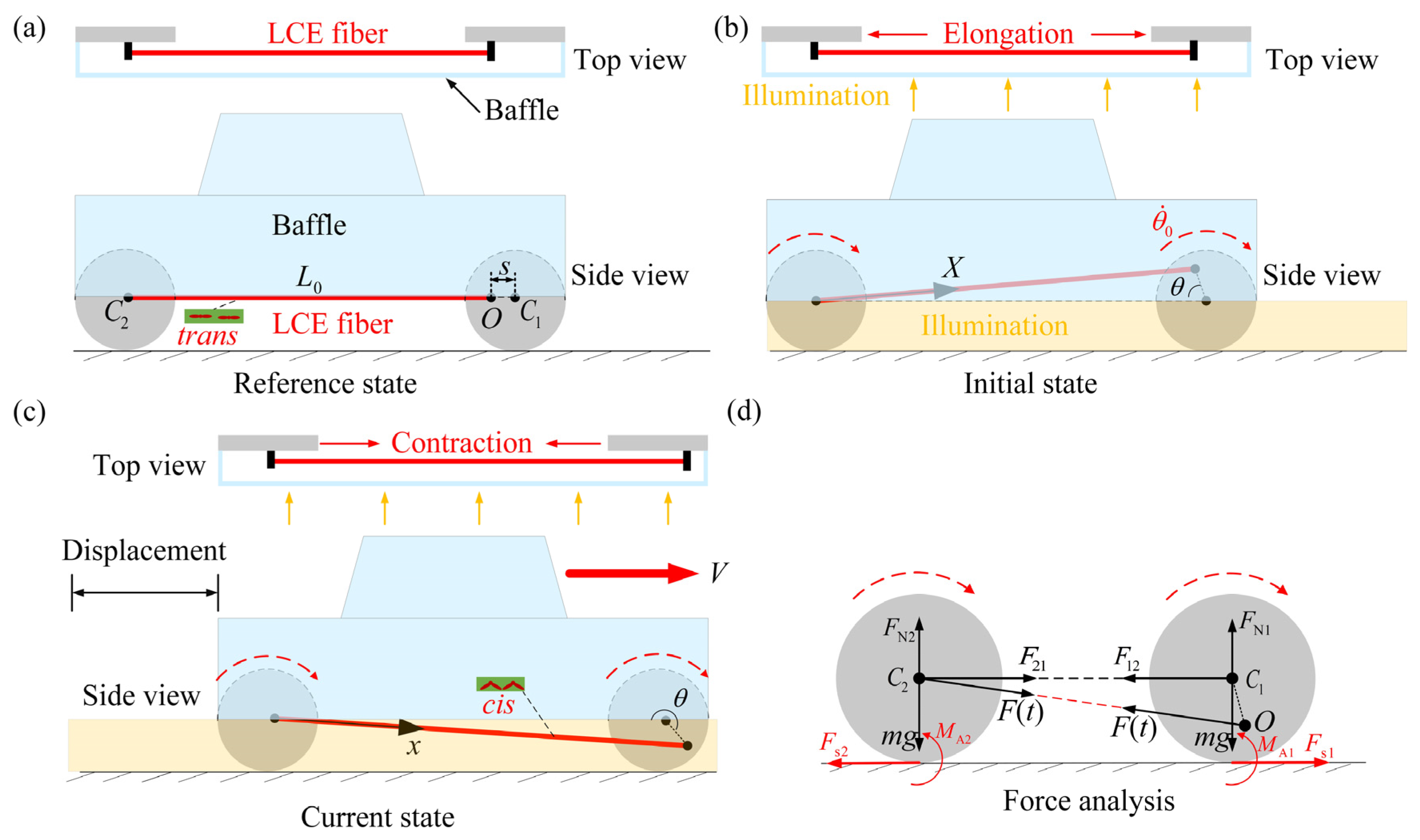
2.1. Dynamics of the Self-Moving LCE-Based Automobile

Figure 1 sketches the LCE-based self-moving automobile, which consists of an LCE fiber and two wheels. Due to the presence of a baffle above the wheels, the area underneath the wheels is steadily illuminated, represented by the yellow area in the Figure 1. One end of the LCE fiber is attached to point O at a distance of s from the center C1 of the front wheel, with s being less than or equal to the wheel radius R, and the other end is attached to the center C2 of the rear wheel. The distance from fixed end O to the wheel center and the wheel center are not in the same plane, which means that the LCE fiber does not wind around the wheel during rotation. As shown in Figure 1a, the LCE fiber is unstressed and has an original length of $L_0$, the nematic LCE fiber contains photosensitive molecules, such as azobenzene molecules, which align themselves along the fiber axis. As a well-established phenomenon, when exposed to light, the LCE fibers undergo contraction as the azobenzene liquid crystal molecules transform from a straight trans state to a bent cis state. Conversely, in darkness, the photo-responsive contraction is reversed as the azobenzene liquid crystal molecules transform from a bent cis state back to a straight trans state, leading to recovery [19,54]. Initially, the LCE-based automobile obtains an initial angular velocity ${\overline{\dot{\theta }}}_0$ from the reference state, and the LCE fibers begin self-rotation, driving the wheels to roll (Figure 1b). At the beginning of the wheels rolling, the azobenzene liquid crystal molecules in the LCE fiber remain in the straight trans state, and then, as the wheels rotate, the LCE fiber begins to enter the illumination zone, the azobenzene liquid crystal molecules transform from the straight trans state to the bent cis state, and the LCE fiber contracts under illumination (Figure 1c). Figure 1d gives the force analysis of the automobile.

The photo-responsive contraction increases the tension $F\left(t\right)$ and the rotational moment $M_{\mathrm{F}}\left(t\right)$. Due to the transformation of azobenzene liquid crystal molecules from a straight trans state to a bent cis state under illumination, as the wheels roll forward, the LCE fiber contracts under illumination, so the $F\left(t\right)$ of the LCE fiber is amplified through the photo-responsive contraction. The friction $F_{\mathrm{s}1}$ and $F_{\mathrm{s}2}$ between the front and rear wheels and the horizontal surface generates the rolling moments $M_{\mathrm{s}1}$ and $M_{\mathrm{s}2}$. At the same time, the rolling damping moments $M_{\mathrm{A}1}$ and $M_{\mathrm{A}2}$ are generated between the wheels and the horizontal surface as the wheels roll, which makes the wheels always tend to rotate in the reverse direction. As the rolling angle of the wheels increases, the light energy absorbed by the LCE fiber progressively increases, and the $F\left(t\right)$ also increases. Subsequently, the automobile speed decreases and the automobile continues to move forward, the LCE fiber gradually exits the illumination zone, and then the automobile continues to roll past the critical position due to its own inertia. The LCE fiber will contract again by illumination, and move through the illuminated and non-illuminated zones in the same way, and, finally, under steady illumination, the wheels may exhibit continuous periodic motion that propels the automobile to continue to move forward.

As depicted in Figure 1d, the wheels experience $M_{\mathrm{F}}\left(t\right)$, $M_{\mathrm{s}1}$ $M_{\mathrm{s}2}$, $M_{\mathrm{A}1}$ and $M_{\mathrm{A}2}$. The derivation of the corresponding nonlinear dynamic governing equation for the self-moving automobile can yield the following expression

$$\left\{\begin{array}{c}J\frac{d^2\theta (t)}{d{t}^2}=M_{\mathrm{F}}(t)-M_{\mathrm{A}1}-M_{\mathrm{s}1}\\ J\frac{d^2\theta (t)}{d{t}^2}=-M_{\mathrm{A}2}-M_{\mathrm{s}2}\end{array}\right.,$$

(1)

$$\left\{\begin{array}{c}F\left(t\right)\cos \alpha +F_{\mathrm{s}1}+F_{12}=m{a}_{\mathrm{c}}\\ -F\left(t\right)\cos \alpha +F_{\mathrm{s}2}-F_{21}=m{a}_{\mathrm{c}}\end{array}\right.,$$

(2)

where J is the moment of inertia of the wheels about their center points $C_1$ and $C_2$, $a_{\mathrm{c}}$ is the translational acceleration of the wheels, calculated as $a_{\mathrm{c}}=\frac{d^2\theta (t)}{d{t}^2}R$, $F_{12}$ and $F_{21}$ are the forces between the two wheels with $F_{12}=F_{21}$, $M_{\mathrm{A}1}$ and $M_{\mathrm{A}2}$ are the rolling damping moments of the front and rear wheels, respectively, calculated as $M_{\mathrm{A}1}=\delta \left[mg+F\left(t\right)\sin \alpha \right]$ and $M_{\mathrm{A}2}=\delta \left[mg-F\left(t\right)\sin \alpha \right]$, $F_{\mathrm{s}1}$ and $F_{\mathrm{s}2}$ are frictions between the front and rear wheels and the horizontal surface, respectively, calculated as $F_{\mathrm{s}1}=-F\left(t\right)\cos \alpha -F_1+m{a}_{\mathrm{c}}$ and $F_{\mathrm{s}2}=F\left(t\right)\cos \alpha +F_2+m{a}_{\mathrm{c}}$, and $M_{\mathrm{s}1}$ and $M_{\mathrm{s}2}$ are the rolling moments of the front and rear wheels, respectively, calculated as $M_{\mathrm{s}1}=F_{\mathrm{s}1}R$ and $M_{\mathrm{s}2}=F_{\mathrm{s}2}R$.

The rotational moment, as stated in Equation (1), and its calculation can be expressed as follows:

$$\left\{\begin{array}{l}\begin{array}{cc}{M}_{\mathrm{F}}(t)=-F(t)d& 2n\pi \le \theta \le \pi +2n\pi \end{array}\\ \begin{array}{cc}{M}_{\mathrm{F}}(t)=F(t)d& \pi +2n\pi \le \theta \le 2\pi +2n\pi \end{array}\end{array}\right.,$$

(3)

where d is the lever.

By amalgamating the rolling damping moments of the front and rear wheels, as well as the rolling moments of the front and rear wheels, respectively, and denoting them as $M_{\mathrm{A}}$ and $M_{\mathrm{s}}$:

$$\left\{\begin{array}{l}{M}_{\mathrm{A}}=2\delta mg\\ M_{\mathrm{s}}=2m{a}_{\mathrm{c}}R\end{array}\right.,$$

(4)

where $\delta$ is the rolling resistance coefficient and $g$ is the gravitational acceleration.

Adding the two formulas of Equation (1) and substituting Equation (4) into Equation (1), Equation (1) can be rewritten as

$$2J\ddot{\theta }=M_{\mathrm{F}}\left(t\right)-2\delta mg\frac{\dot{\theta }}{\left|\dot{\theta }\right|}-2m{a}_{\mathrm{c}}R.$$

(5)

The length of the LCE fiber $L(t)=\sqrt{s^2+{(L_0+s)}^2-2s(s+L_0)\cos \theta }$ and the lever $d\left(t\right)=\left(L_0+s\right)s\sin \theta /L\left(t\right)$.

2.2. Tension of the LCE Fiber

In order to obtain the $M_{\mathrm{F}}\left(t\right)$ in Equation (3), the $F\left(t\right)$ needs to be calculated. To simplify the analysis, the friction and mass of the LCE fiber are disregarded. To simplify, the elastic strain ${\epsilon }_{\mathrm{e}}\left(t\right)$ in the LCE fiber under small deformation can be considered as a linear combination of the ${\epsilon }_{\mathrm{tot}}\left(t\right)$ and the ${\epsilon }_{\mathrm{L}}\left(t\right)$, i.e., ${\epsilon }_{\mathrm{tot}}(t)={\epsilon }_{\mathrm{e}}(t)+{\epsilon }_{\mathrm{L}}(t)$, assuming that the $F\left(t\right)$ is proportional to the elastic strain, that is:

$$F(t)=k{L}_0\left[{\epsilon }_{\mathrm{tot}}(t)-{\epsilon }_{\mathrm{L}}(t)\right],$$

(6)

where k represents the spring constant. It is important to mention that the LCE fiber exhibits homogeneity, while both the ${\epsilon }_{\mathrm{tot}}\left(t\right)$ and ${\epsilon }_{\mathrm{L}}\left(t\right)$ are heterogeneous. In order to examine the heterogeneous deformation of the LCE fiber, two coordinate systems are introduced: the Lagrangian arc coordinate system X in the reference state (Figure 1a) and the Eulerian arc coordinate system x in the current state (Figure 1c). The position of a material point in the LCE fiber during the rolling process of the wheels can be represented as x = x(X,t).

It is assumed that the total strain ${\epsilon }_{\mathrm{L}}\left(X,t\right)$ is linearly dependent on the number fraction of cis-isomers $\varphi \left(t\right)$. The photo-responsive contraction is then determined as

$${\epsilon }_{\mathrm{L}}(t)=-C_0\varphi (t),$$

(7)

where $C_0$ is the contraction coefficient. For simplicity, the total strain is defined as ${\epsilon }_{\mathrm{tot}}(t)=\frac{L(t)-L_0}{L_0}$ [58].

Thus, the $F\left(t\right)$ in Equation (6) can be rewritten as

$$F(t)=k\left[(L(t)-L_0)+C_0{L}_0\varphi (t)\right].$$

(8)

2.3. Dynamic LCE Model

The calculation of the number fraction $\varphi \left(t\right)$, as described in Equation (9), relies on the utilization of the established dynamic LCE model proposed by Finkelmann et al. [59,60]. Yu et al. discovered that the trans-to-cis isomerization of LCE can be triggered by ultraviolet light or a laser with a wavelength below 400 nm [61]. The determination of the $\varphi \left(t\right)$ is influenced by three factors: thermal excitation causing a transition from trans to cis, thermally driven relaxation leading to a transition from cis to trans, and optically driven relaxation inducing a transition from trans to cis. However, in many cases, the thermal excitation from trans to cis is considered insignificant compared to the photo-responsive excitation [60], therefore, the $\varphi \left(t\right)$ can be represented as

$$\frac{\partial \varphi (t)}{\partial t}={\eta }_0{I}_0\left[1-\varphi (t)\right]-{\tau }_0^{-1}\varphi (t),$$

(9)

where ${\tau }_0$ is the thermal relaxation time from cis to trans, $I_0$ is the light intensity, and ${\eta }_0$ is the light absorption constant. Given that the number fraction of cis-isomers at t = 0 is denoted as ${\varphi }_0$, taking into account the initial number fraction (${\varphi }_0=0$), in the presence of the LCE fiber within the illumination zone, the accurate representation of the number fraction of cis-isomers can be obtained

$${\varphi }_1(t)=\frac{{\eta }_0{\tau }_0{I}_0}{{\eta }_0{\tau }_0{I}_0+1}+(1-\frac{{\eta }_0{\tau }_0{I}_0}{{\eta }_0{\tau }_0{I}_0+1})\exp [-\frac{t}{{\tau }_0}({\eta }_0{\tau }_0{I}_0+1)].$$

(10)

Conversely, when the LCE fiber is in the non-illumination zone, the number fraction of cis-isomers can also be expressed as

$${\varphi }_2(t)=\frac{{\eta }_0{\tau }_0{I}_0}{{\eta }_0{\tau }_0{I}_0+1}\exp (-\frac{t}{{\tau }_0}).$$

(11)

2.4. Nondimensionalization

For convenience, the following dimensionless quantities are introduced: $\overline{t}=t/{\tau }_0$, $\overline{L}=L/L_0$, $\overline{R}=R/L_0$, $\overline{X}=X/L_0$, $\overline{x}=x/L_0$, $\overline{d}=d/L_0$, ${\overline{M}}_{\mathrm{F}}\left(\overline{t}\right)=M_F\left(t\right){\tau }_0^2/J$, $\overline{F}\left(\overline{t}\right)=F\left(t\right)L_0{\tau }_0^2/J$, $\overline{k}=k{\tau }_0^2{L}_0^2/J$, $\overline{I}=I{\eta }_0{\tau }_0$, ${\overline{I}}_0=I_0{\eta }_0{\tau }_0$, $\overline{\delta }=\delta /L_0$, $\overline{g}=g{\tau }_0^2/L_0$, and $\overline{s}=s/L_0$. Equations (5), (8), (10) and (11) can be rewritten as follows:

$$\ddot{\theta }\left(\overline{t}\right)={\overline{M}}_{\mathrm{F}}\left(\overline{t}\right)/3-\left(\overline{\delta }\overline{g}/3{\overline{R}}^2\right)\frac{\overline{\dot{\theta }}}{\left|\overline{\dot{\theta }}\right|}.$$

(12)

For simplicity, $\overline{\delta }\overline{g}$ is reduced to A, which denotes the rolling resistance coefficient, and ${\overline{M}}_{\mathrm{A}}=A/3{\overline{R}}^2$.

The dimensionless form for the tension $\overline{F}(\overline{t})$ of the LCE fiber is

$$\overline{F}(\overline{t})=\overline{k}\left[(\overline{L}(\overline{t})-1)+C_0\varphi (\overline{t})\right],$$

(13)

where $\overline{L}(\overline{t})=\sqrt{{\overline{s}}^2+{(1+\overline{s})}^2-2\overline{s}(\overline{s}+1)\cos \theta }$ and $\overline{d}=\left(1+\overline{s}\right)\overline{s}\sin \theta /\overline{L}\left(\overline{t}\right)$.

The nondimensionalized equation for the number fraction of cis-isomers is derived as follows:

in the illumination zone

$${\varphi }_1(\overline{t})=1-\exp [-\overline{t}({\overline{I}}_0+1)];$$

(14)

in the non-illumination zone

$${\varphi }_2(\overline{t})=\exp (-\overline{t}).$$

(15)

Through Equations (14) and (15), the $\varphi (\overline{t})$ can be calculated. As the LCE fiber transitions across the boundary separating the illumination and non-illumination zones, the time-dependent behavior of the $\varphi (\overline{t})$ alternates between Equations (14) and (15). To calculate these intricate dimensionless equations, the Runge-Kutta method is employed, and numerical computations are conducted using MATLAB R2016b software. For the number fraction ${\varphi }_{\mathrm{i}}$ of cis-isomers and the position ${\theta }_{\mathrm{i}}$ of the wheels at time $t_{\mathrm{i}}$, the current tensions $F_{\mathrm{i}}$ and the current rotational moment ${\overline{M}}_{\mathrm{Fi}}$ can be calculated by Equations (12) to (13). Then the angular position of the wheels ${\theta }_{\mathrm{i}+1}$ at time ${\overline{t}}_{\mathrm{i}+1}$ can be calculated using Equation (12).

3. Two Motion Regimes and Mechanism of Self-Moving

In the above process, the governing Equations (12) and (13) of LCE-based automobile are derived. Next, the two motion regimes of the LCE-based automobile will be discussed, and the mechanism of each motion regime will be analyzed in depth.

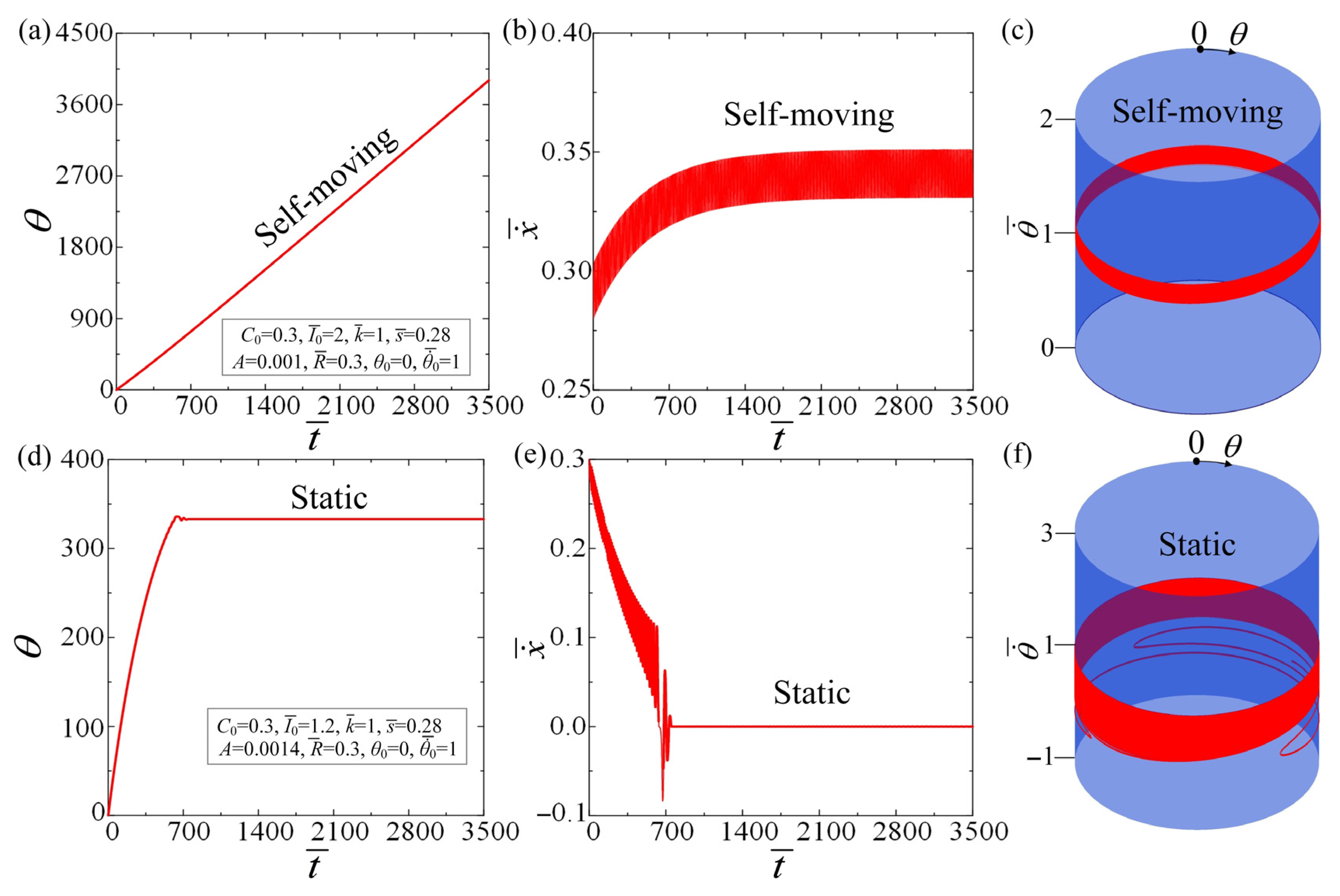
3.1. Two Motion Regimes

In order to analyze the behavior of the self-moving LCE-based automobile under steady illumination, it is necessary to establish the reference values of the dimensionless parameters. These values can be determined based on the material properties and geometric parameters obtained from the available experiments [18,62,63,64].

Table 1. Material properties and geometric parameters.

Parameter	Definition	Value	Unit
A	Rolling resistance coefficient	0~0.01	mm/s2
C0	Contraction coefficient	0~0.2	/
${\eta }_0$	Light-absorption constant	0.0003	m2/(s·W)
${\tau }_0$	Thermal relaxation time from cis-to-trans	0~100	ms
J	Moment of inertia of the wheels	0~1	mg·mm2
I0	Light intensity	0~100	kW/m2
k	Spring coefficient of the LCE fiber	0~2	N/m
R	Wheel radius	0.28~0.5	mm
s	Distance from fixed end to wheel center	0.1~0.3	mm
$L_0$	Original length of LCE fiber	0.1	m

presents the reference values for these properties, while

Table 2. Dimensionless parameters.

Parameter	${\mathit{\theta }}_0$	${\dot{\overline{\mathit{\theta }}}}_0$	${\overline{\mathit{I}}}_0$	$\mathit{A}$	$\overline{\mathit{k}}$	$\overline{\mathit{R}}$	${\mathit{C}}_0$	$\overline{\mathit{s}}$
Value	0	0~10	0~3	0~0.01	0~2	0.28~0.5	0~0.3	0.1~0.3

lists the corresponding dimensionless parameters.

Figure 2 and Movie S1 present the two typical motion regimes that can be achieved in the automobile system, namely the static regime and the self-moving regime. In the calculation, the initial parameter is set to $C_0=0.3$, ${\overline{I}}_0=2$, $\overline{k}=1$, $A=0.001$, $\overline{R}=0.3$, $\overline{s}=0.28$, ${\theta }_0=0$, and ${\overline{\dot{\theta }}}_0=1$. The LCE fiber is stimulated by illumination to undergo periodic self-rotation, which acts like an engine to propel the automobile forward. Driven by the self-rotation of the LCE fiber, the automobile gradually moves forward to self-propel, and after a period of time, the self-rotation frequency of the LCE fiber, as well as the self-moving frequency of the automobile, tend to be steady, which is defined as the self-moving regime. Next, the parameter is set to $C_0=0.3$, ${\overline{I}}_0=1.2$, $\overline{k}=1$, $A=0.0014$, $\overline{R}=0.3$, $\overline{s}=0.28$, ${\theta }_0=0$, and ${\overline{\dot{\theta }}}_0=1$. The self-rotation frequency of the LCE fiber gradually decreases and eventually comes to a stationary state. Influenced by this, the velocity of the automobile directly decreases. When the LCE fiber stops rotating, the velocity of the automobile drops to 0 and stops there, which is the static regime. As shown in Figure 2c,f, as the parameters ${\overline{I}}_0$ and $A$ vary, a stable fixed point loses stability and gives rise to a stable limit cycle. This means that the system transitions from a stable static state to periodic oscillations, which is the characteristic of a supercritical Hopf bifurcation [65]. As shown in Section 4, this paper will additionally explore the mechanism of the self-moving automobile in a detailed study.

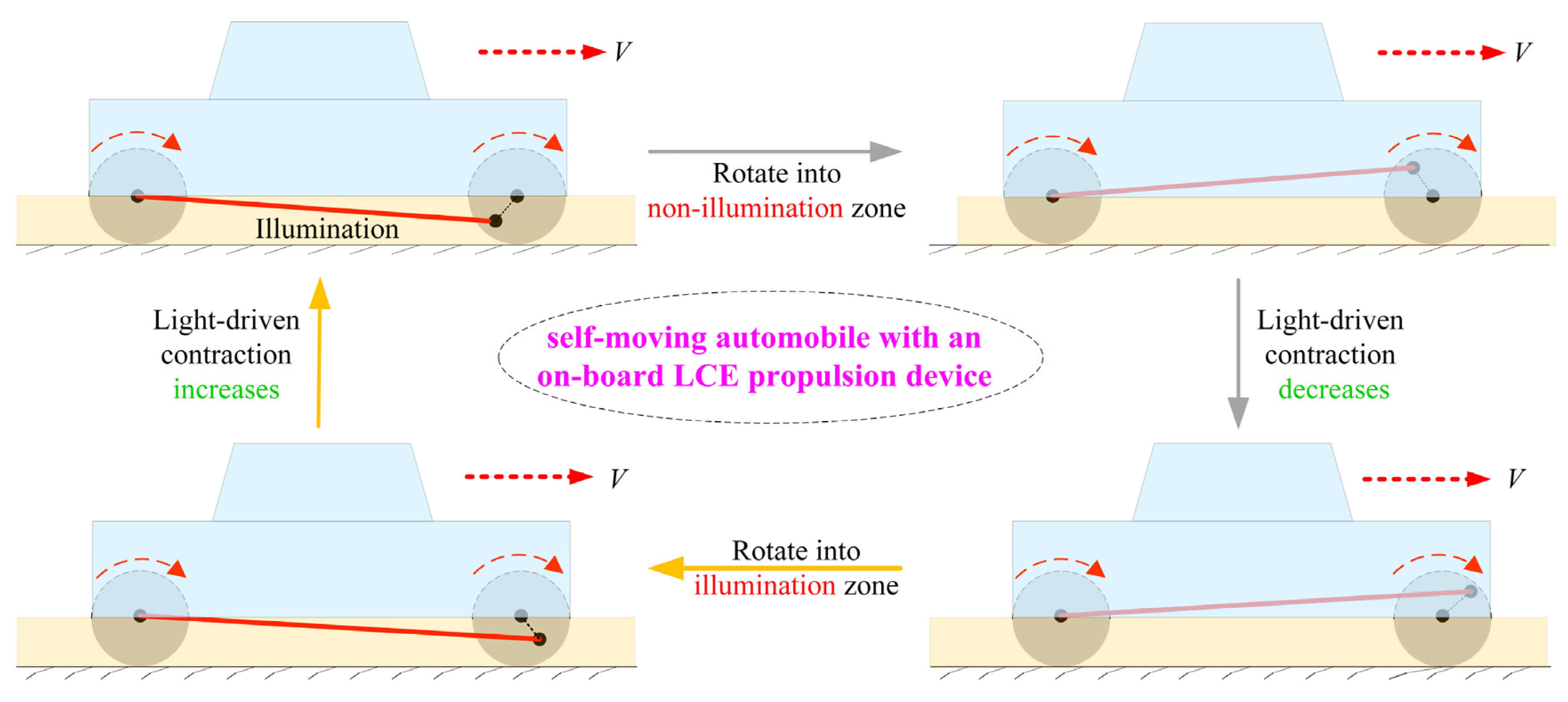
3.2. Mechanism of Self-Moving

This subsection mainly focuses on the mechanism of self-moving for the LCE-based automobile under steady illumination. Figure 3a–c provide the time dependances for the $\varphi$, the $\overline{L}$, and the $\overline{F}$ of the LCE fiber, and the yellow region in the figure represents the illumination zone. For the numerical calculations, the following assumptions are made: $C_0=0.3$, ${\overline{I}}_0=2$, $\overline{k}=1$, $A=0.0014$, $\overline{R}=0.3$, $\overline{s}=0.28$, ${\theta }_0=0$, and ${\overline{\dot{\theta }}}_0=1$. As depicted in Figure 3a, the number fraction of cis-isomers in the LCE exhibits a gradual increase inside the illumination zone, followed by a decrease within the non-illumination zone. The periodic fluctuation of the number fraction with respect to time indicates the cyclical change in the photo-responsive strain. From Figure 3b, it can be seen that the $\overline{L}$ also exhibits periodic variations. Eventually, the fiber length varies periodically with time during one cycle of the self-moving regime, which can be further understood from Figure 4. In Figure 3c, it can be observed that the tension of the LCE fiber exhibits an increasing trend over time within the illumination zone. Conversely, in the dark zone, the tension initially decreases and then increases.

Figure 3d shows the variations in $\overline{F}$ and $\theta$ over one cycle. During the self-rotation of LCE fiber, as the fiber enters the illumination zone the increase in $\overline{F}$ is due to the photo-responsive contraction strain. As the LCE fiber enters the non-illumination zone, the $\overline{F}$ within the fiber exhibits a monotonic decrease owing to the decline in photo-responsive contraction strain. Figure 3e shows the relationship between ${\overline{M}}_{\mathrm{F}}$ and $\theta$. The ${\overline{M}}_{\mathrm{F}}$ is jointly controlled by the $\overline{F}$ and $\theta$. The numerical calculation yields a positive net work performed by the driving force from the LCE fiber, which is represented by the area enclosed by the curve in Figure 3e and is determined to be 0.0232. Figure 3f shows the relationship between ${\overline{M}}_{\mathrm{A}}$ and $\theta$, in which the enclosed loop represents the damping dissipation with a value of 0.0232. The net work is equal to the damping dissipation, which implies that the self-rotation of the LCE fiber is a consequence of the interplay between the net work performed by the driving force and the damping dissipation. Therefore, the automobile realizes self-moving due to the self-rotation of the LCE fiber.

4. Influences of System Parameters on the Self-Moving

The two motion regimes of the LCE-based automobile system and the mechanism of the self-moving regime are summarized in the above discussions. The execution of these principles is governed by seven dimensionless physical parameters, which encompass ${\overline{\dot{\theta }}}_0$, ${\overline{I}}_0$, $\overline{k}$, $\overline{R}$, $\overline{s}$, $C_0$, and $A$. In the computation, the parameters are set to be ${\overline{\theta }}_0=0$. By adjusting these parameters, the LCE engine evolves into self-rotation, and then the automobile can realize continuous self-moving. In the current subsection, the effects of these seven parameters on both the Hopf bifurcation conditions and the average velocity V of the automobile will be examined.

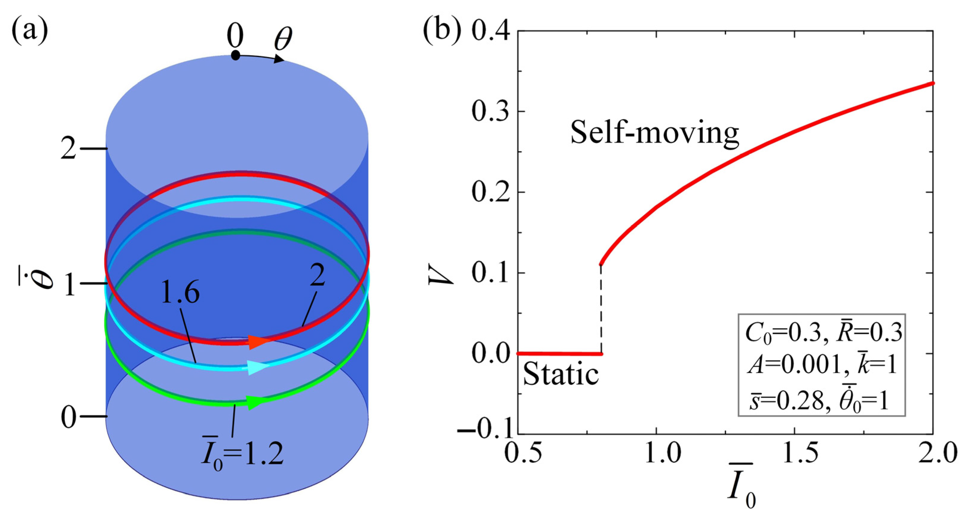
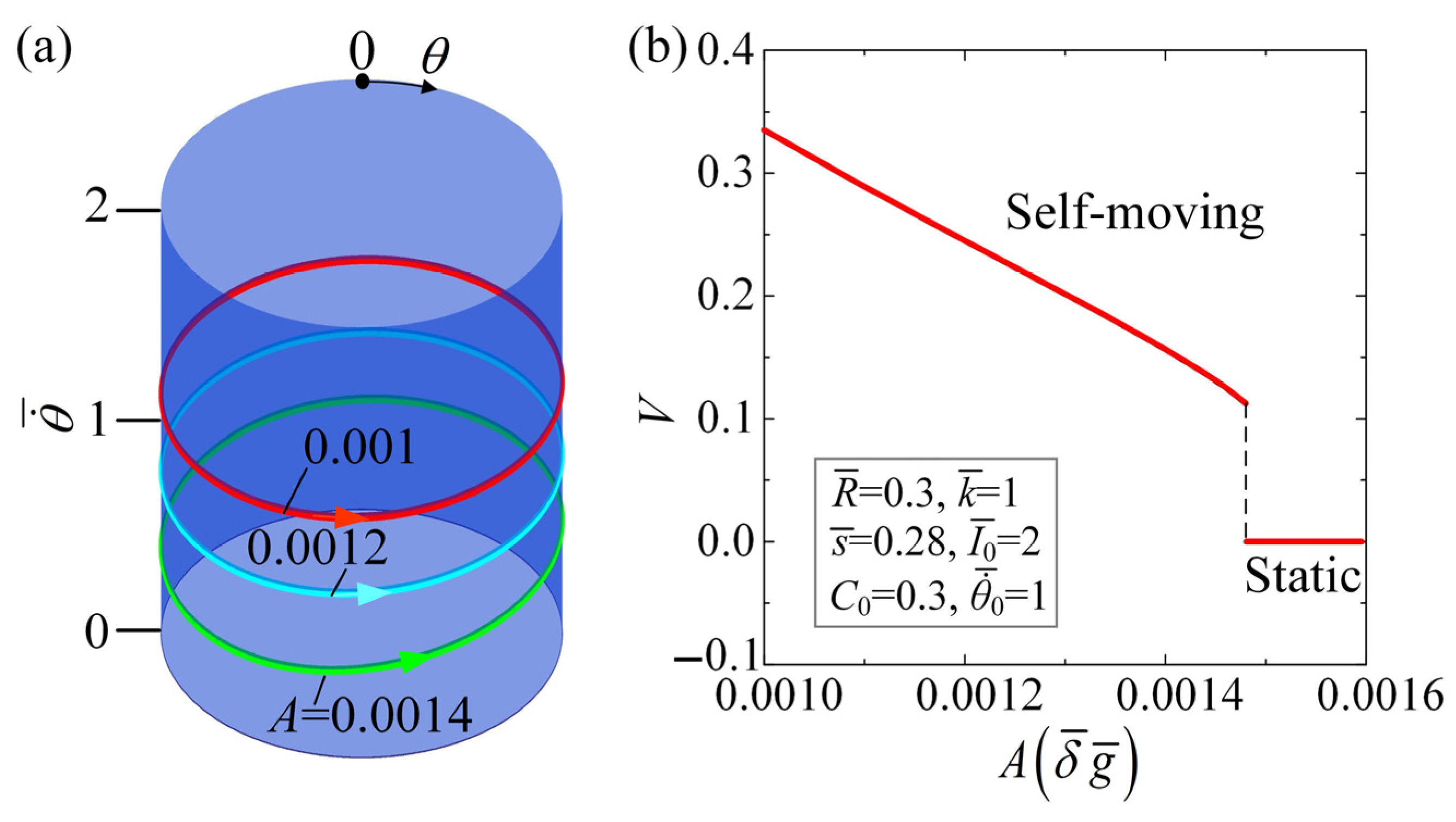
4.1. Effect of the Light Intensity

Figure 5 and Movie S2 illustrate the effect of light intensity ${\overline{I}}_0$ on the self-moving of the LCE-based automobile. The parameters are set for $C_0=0.3$, $\overline{k}=1$, $A=0.001$, $\overline{R}=0.3$, $\overline{s}=0.28$, and ${\overline{\dot{\theta }}}_0=1$. At an approximate value of 0.792 for the light intensity, a critical threshold is reached, triggering the self-rotation of the LCE fiber and enabling the self-moving of the automobile. This indicates that the automobile undergoes a supercritical Hopf bifurcation when the light intensity reaches this critical value. When ${\overline{I}}_0\le 0.792$, the LCE fiber stays stationary, causing the automobile to remain stationary, while when ${\overline{I}}_0=$ 1.2, 1.6, 2, the self-moving regime can be triggered. Figure 5a plots the limit cycles, and Figure 5b shows the effect of ${\overline{I}}_0$ on the average velocity V of the self-moving automobile. With the increase in ${\overline{I}}_0$, the average velocity of the automobile increases gradually. The precise explanation for this outcome is that the photo-responsive contraction of LCE intensifies as parameter ${\overline{I}}_0$ increases, which provides the system with sufficient driving force to perform net work. The light intensity is proved to enable the LCE fiber to rotate faster, thereby accelerating the propulsion velocity of the automobile. In engineering applications, the self-rotation of the LCE fiber and the self-moving of the automobile can be facilitated by adjusting the light intensity.

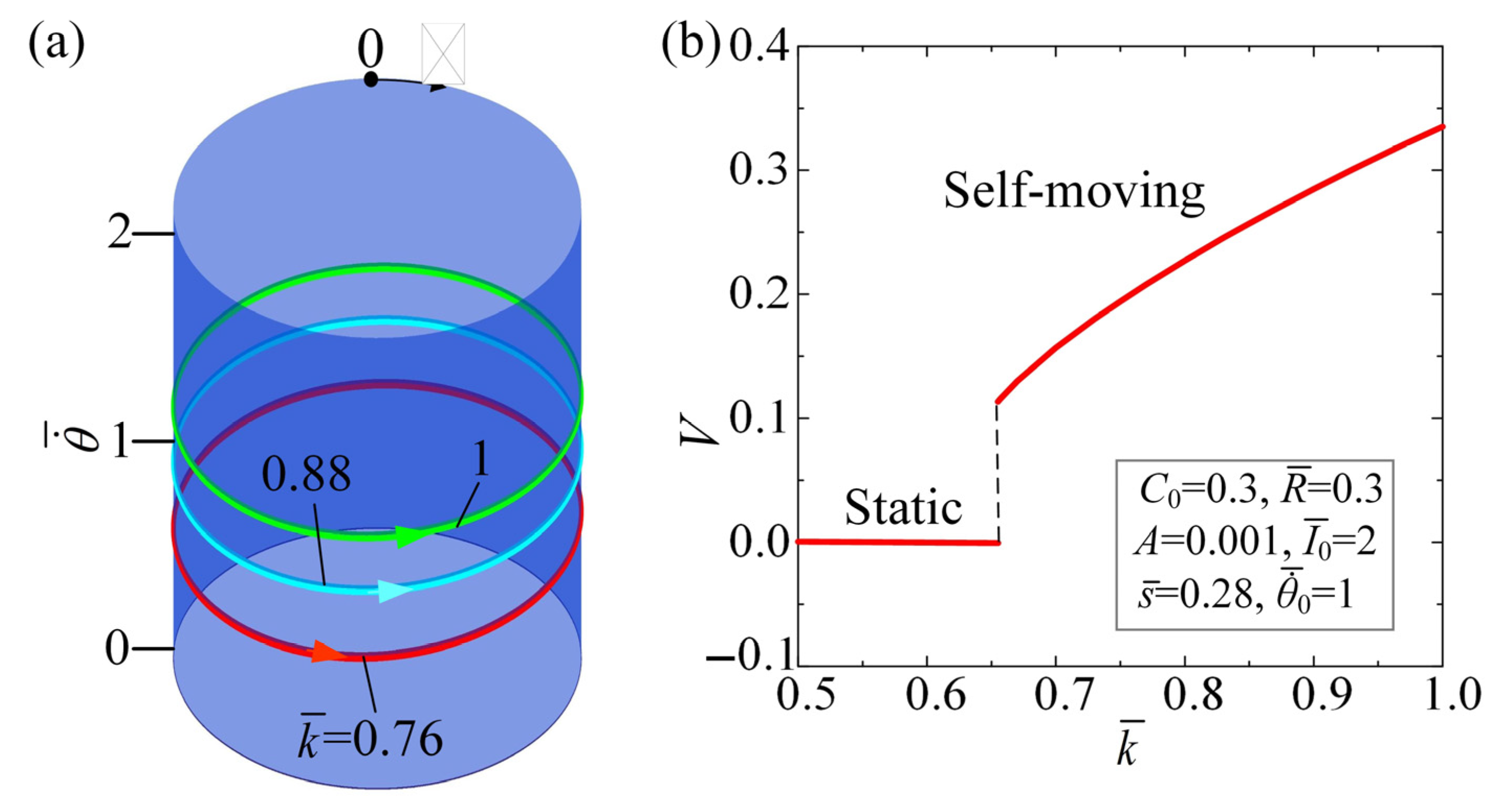
4.2. Effect of the Spring Constant

Figure 6 and Movie S3 describe the effect of spring constant $\overline{k}$ on the self-moving of the LCE-based automobile. Figure 6a depicts the limit cycles for different $\overline{k}$, and Figure 6b displays the relationship between $\overline{k}$ and V of the self-moving automobile. The parameters are set for $C_0=0.3$, ${\overline{I}}_0=2$, $A=0.001$, $\overline{R}=0.3$, $\overline{s}=0.28$, and ${\overline{\dot{\theta }}}_0=1$. A critical value of $\overline{k}$ approximately equal to 0.653 is present for the supercritical Hopf bifurcation between the static regime and the self-moving regime. When $k\le 0.653$, the smaller $\overline{F}$ results in less net work carried out by the ${\overline{M}}_{\mathrm{F}}$, which, consequently, cannot balance the energy dissipated by the damping, and thus, fails to sustain the self-rotation of the LCE fiber and the self-moving of the automobile. Figure 6b presents the increasing trend of average velocity with the increasing $\overline{k}$. The $\overline{F}$ and ${\overline{M}}_{\mathrm{F}}$ of the LCE fiber also increase as the $\overline{k}$ increases. From Equation (6), it can be seen that the effects of ${\overline{I}}_0$ and $\overline{k}$ on tension are similar, as shown in Figure 5 and Figure 6. Given the physical significance of parameter $\overline{k}$, augmenting the $\overline{k}$ can enhance the efficacy of converting light energy into mechanical energy, thereby facilitating more efficient utilization in various engineering applications.

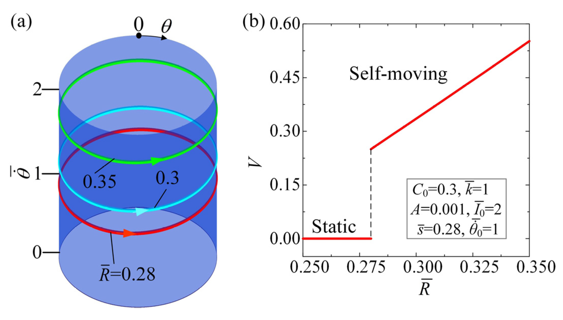
4.3. Effect of the Wheel Radius

Figure 7 and Movie S4 demonstrate the impact of wheel radius $\overline{R}$ on the self-moving of the automobile, for $C_0=0.3$, ${\overline{I}}_0=2$, $A=0.001$, $\overline{k}=1$, $\overline{s}=0.28$, and ${\overline{\dot{\theta }}}_0=1$. In Figure 7a, the limit cycles for varying wheel radius are depicted, and Figure 7b presents the relationship between $\overline{R}$ and average velocity V of the self-moving automobile. A critical $\overline{R}$ of 0.28 is present to trigger the self-rotation of the LCE fiber and the self-moving of the automobile. Since the distance from the fixed end to the wheel center is set as 0.28 in the initial condition, the wheel radius cannot be smaller than this distance, thus only cases where the radius is greater than or equal to 0.28 are considered. When the radius is reduced, the tension in the LCE fiber decreases, resulting in insufficient net work carried out by the rotational moment to counterbalance the damping dissipation. As a result, it becomes inadequate to sustain the self-rotation of the LCE fiber and the self-moving of the automobile. The upward trend of the average velocity with the increasing $\overline{R}$ is given in Figure 7b. The derivations show that the $\overline{F}$ and the ${\overline{M}}_{\mathrm{F}}$ increase as the $\overline{R}$ increases. This finding suggests that the increase in wheel radius can improve the self-rotation of the LCE fiber and the self-moving of the automobile under steady illumination.

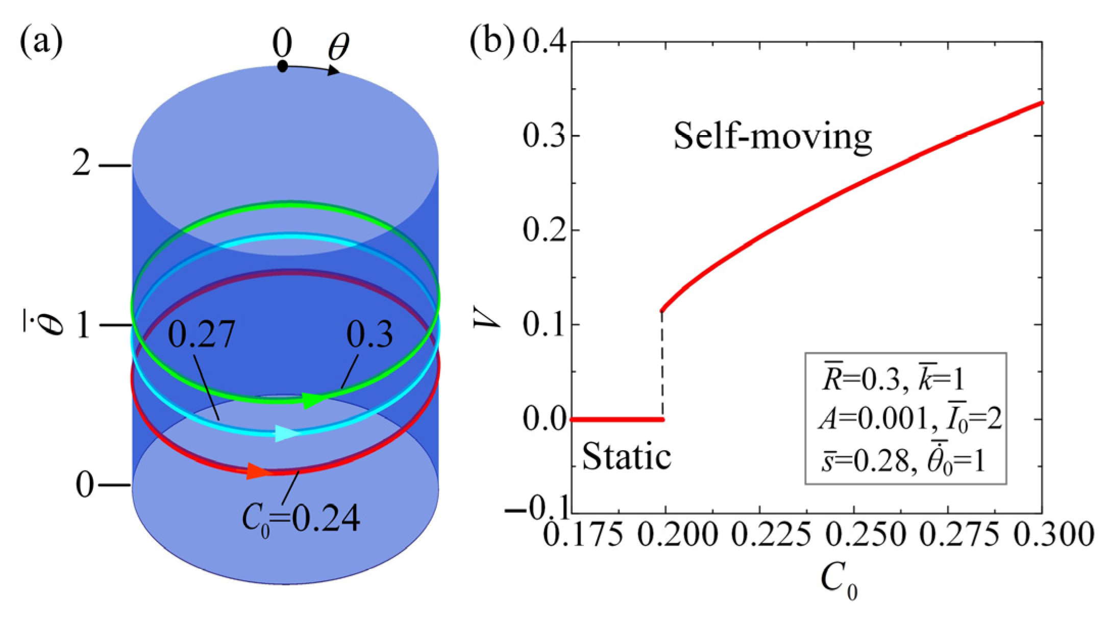
4.4. Effect of the Contraction Coefficient

Figure 8 and Movie S5 display the effect of contraction coefficient $C_0$ on the self-moving of the automobile, for ${\overline{I}}_0=2$, $A=0.001$, $\overline{k}=1$, $\overline{R}=0.3$, $\overline{s}=0.28$, and ${\overline{\dot{\theta }}}_0=1$. Similarly, a critical $C_0$ approximately equal to 0.198 exists for triggering the self-rotation of the LCE fiber and the self-moving of the automobile. The LCE-based automobile remains static when $C_0\le 0.198$, while for $C_0=$ 0.24, 0.27, and 0.3, the self-moving regime can be triggered, with limit cycles being plotted in Figure 8a. Figure 8b describes the effect of $C_0$ on the average velocity V of the self-moving automobile. As $C_0$ increases, the average velocity of the self-moving automobile tends to increase. Equation (7) demonstrates that augmenting the $C_0$ results in an upsurge in the photo-responsive strain, which corresponds to a corresponding increase in the absorbed light energy. This infers that raising the $C_0$ can improve the efficiency of converting light energy into mechanical energy.

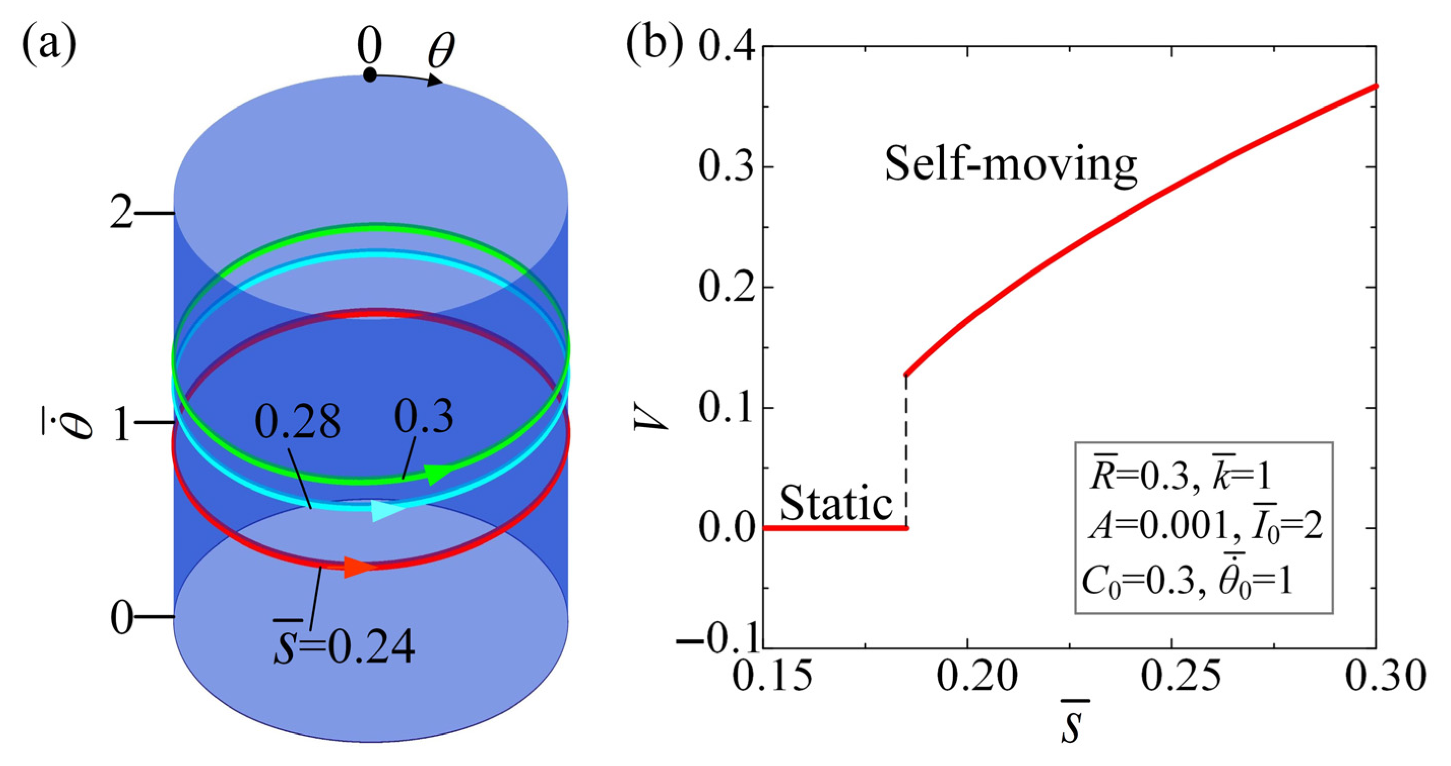
4.5. Effect of the Distance from Fixed End to Wheel Center

Figure 9 and Movie S6 present the influence of distance $\overline{s}$ from fixed end to wheel center on the self-moving of the automobile, for $C_0=0.3$, ${\overline{I}}_0=2$, $A=0.001$, $\overline{k}=1$, $\overline{R}=0.3$, and ${\overline{\dot{\theta }}}_0=1$. Similarly, the critical distance $\overline{s}$ from fixed end to wheel center, which is approximately equal to 0.18, is present to trigger the self-rotation of the LCE fiber and the self-moving of the automobile. When $\overline{s}\le 0.18$, the LCE-based automobile remains in static regime. For $\overline{s}=$ 0.24, 0.28, and 0.3, the automobile exhibits the self-moving regime, and their limit cycles are depicted in Figure 9a. It is worth noting that when the wheel radius is $\overline{R}=0.3$, the distance from fixed end to wheel center cannot exceed the wheel radius; therefore, the value range of this distance is less than or equal to 0.3. Figure 9b illustrates the effect of the distance from fixed end to wheel center on the average velocity of the self-moving automobile. As $\overline{s}$ increases, the average velocity trends upwards. Increasing the distance from fixed end to wheel center will cause an increase in the lever $\overline{d}$, which will in turn induce increases in the $\overline{F}$ and the ${\overline{M}}_{\mathrm{F}}$ of the wheels. This result suggests that increasing the distance from fixed end to wheel center will be beneficial in improving the self-rotation of the LCE fiber and the self-moving of the automobile under steady illumination.

4.6. Effect of the Rolling Resistance Coefficient

Figure 10 and Movie S7 describe the influence of rolling resistance coefficient $A$ on the self-moving of the automobile. Figure 10a illustrates the limit cycles for different rolling resistance coefficients, while Figure 10b expresses the average velocity V of the self-moving automobile as a function of the $A$. In the calculation, the parameters are set for $C_0=0.3$, ${\overline{I}}_0=2$, $\overline{k}=1$, $\overline{R}=0.3$, $\overline{s}=0.28$, and ${\overline{\dot{\theta }}}_0=1$. A critical value of $A$, which is approximately 0.0015, is present to trigger the self-rotation of the LCE fiber and the self-moving of the automobile. When $A\ge 0.0015$, the absorbed light energy is insufficient to compensate for the excessive damping dissipation, causing the automobile to enter a static regime. However, for $A=0.0014$, $A=0.0012$, and $A=0.001$, the self-rotation of the LCE fiber and the self-moving of the automobile can be triggered. An increase in the rolling resistance coefficient leads to a decrease in the average velocity of the self-moving automobile. Based on the aforementioned derivation process, it can be concluded that as the rolling resistance coefficient increases, the LCE fiber requires more energy to overcome damping, resulting in a reduction in the average velocity of the self-moving automobile.

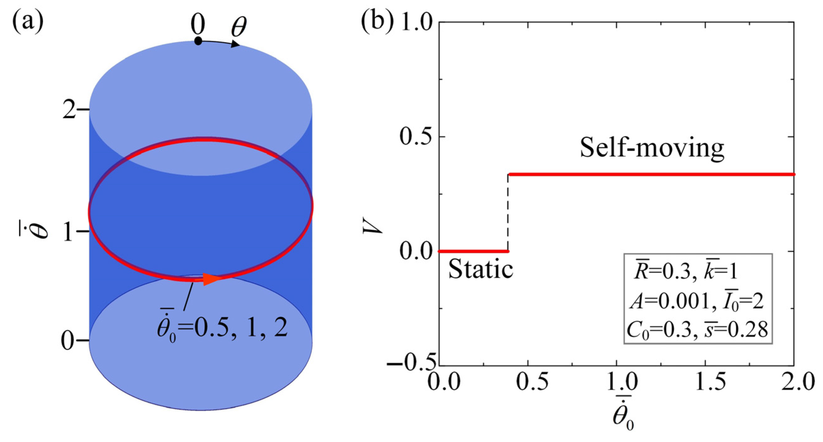
4.7. Effect of the Initial Velocity

Figure 11 and Movie S8 illustrate the effect of initial velocity ${\overline{\dot{\theta }}}_0$ on the self-moving of the automobile. The parameters are set for $C_0=0.3$, $\overline{k}=1$, ${\overline{I}}_0=2$, $A=0.001$, $\overline{R}=0.3$, and $\overline{s}=0.28$. In Figure 11a, the limit cycles for various initial velocities are depicted, while Figure 11b illustrates the relationship between the average velocity V of the self-moving automobile and the ${\overline{\dot{\theta }}}_0$. As shown in Figure 11a,b, the ${\overline{\dot{\theta }}}_0$ has no influence on the limit cycle and the average velocity of the self-moving automobile. From the numerical calculations, a critical ${\overline{\dot{\theta }}}_0$ of roughly 0.357 exists between the static regime and the self-moving regime. The self-rotation of the LCE fiber and the self-moving of the automobile are triggered at initial velocities of 0.5, 1, and 2. Taking into account the equivalency between kinetic and potential energies during the conversion of ${\overline{\theta }}_0$ and ${\overline{\dot{\theta }}}_0$, the initial conditions are irrelevant on the average velocity of the self-moving automobile, which is a fundamental characteristic of self-oscillation [66].

5. Conclusions

To overcome the disadvantage of traditional active machines requiring complex control systems, this paper develops an innovative self-moving LCE-based automobile under steady illumination, featuring an LCE fiber and two wheels. Utilizing the dynamic LCE model, a theoretical framework for the LCE-based automobile is proposed to investigate its self-oscillatory behaviors. Through numerical simulations, this paper has demonstrated that the automobile, propelled by the LCE fiber, experiences a supercritical Hopf bifurcation, transitioning from a static state to a self-moving mode. The self-moving mechanism of the LCE-based automobile is attributed to the light-induced contraction of the LCE fiber in response to illumination, where light energy offsets damping dissipation in cyclic motion. Increasing the system parameters, including $C_0$, ${\overline{I}}_0$, $\overline{k}$, $\overline{R}$, and $\overline{s}$, can improve the self-moving average velocity. Conversely, an increase in $A$ leads to a decrease in the average velocity.

Conclusively, the automobile proposed in this paper can self-move through self-oscillation, and its movement speed can be controlled through system parameters. In the future, this self-moving automobile is worth validating through experiments, and verifying the effectiveness of the equations. It is worth noting that the theoretical analysis overlooks the impact of the viscoelasticity and gravity on LCE fibers, which should be considered in experimental studies. The proposed method of controlling motion through self-oscillation indicates significant advantages, such as integrated sensors and actuators, wireless control, adjustable size, and high energy efficiency. These findings provide guidance for potential applications in the fields of actuators, soft robotics and energy harvesting.

References

1. Brighenti, R.; Artoni, F.; Cosma, M.P. Mechanics of materials with embedded unstable molecules. Int. J. Solids Struct. 2019, 162, 21–35. [Google Scholar] [CrossRef]
2. Chen, Y.F.; Zhao, H.C.; Mao, J.; Chirarattananon, P.; Helbling, F.; Hyun, P.N.; Clarke, D.; Wood, R. Controlled flight of a microrobot powered by soft artificial muscles. Nature 2019, 575, 324–329. [Google Scholar] [CrossRef] [PubMed]
3. Hua, M.; Kim, C.; Du, Y.; Wu, D.; Bai, R.; He, X. Swaying gel: Chemo-mechanical self-oscillation based on dynamic buckling. Matter 2021, 4, 1029–1041. [Google Scholar] [CrossRef]
4. Qi, F.; Li, Y.; Hong, Y.; Zhao, Y.; Qing, H.; Yin, J. Defected twisted ring topology for autonomous periodic flip–spin–orbit soft robot. Proc. Natl. Acad. Sci. USA 2024, 121, e2312680121. [Google Scholar] [CrossRef] [PubMed]
5. Lee, Y.B.; Koehler, F.; Dillon, T.; Loke, G.; Kim, Y.; Marion, J.; Antonini, M.J.; Garwood, I.; Sahasrabudhe, A.; Nagao, K.; et al. Magnetically actuated fiber-based soft robots. Adv. Mater. 2023, 35, 2301916. [Google Scholar] [CrossRef] [PubMed]
6. Liao, W.; Yang, Z. The integration of sensing and actuating based on a simple design fiber actuator towards intelligent soft robots. Adv. Mater. Technol. 2022, 7, 2101260. [Google Scholar] [CrossRef]
7. Cheng, Y.C.; Lu, H.C.; Lee, X.; Zeng, H.; Priimagi, A. Kirigami-based light-induced shape-morphing and locomotion. Adv. Mater. 2020, 32, 1906233. [Google Scholar] [CrossRef] [PubMed]
8. Martella, D.; Nocentini, S.; Parmeggiani, C.; Wiersma, D. Self-regulating capabilities in photonic robotics. Adv. Mater. Technol. 2019, 4, 1800571. [Google Scholar] [CrossRef]
9. Wang, X.; Ho, G.W. Design of untethered soft material micromachine for life-like locomotion. Mater. Today 2022, 53, 197–216. [Google Scholar] [CrossRef]
10. Yoshida, R. Evolution of self-oscillating polymer gels as autonomous soft actuators. In Soft Actuators: Materials, Modeling, Applications, and Future Perspectives; Springer: Berlin/Heidelberg, Germany, 2019; pp. 61–89. [Google Scholar]
11. Wang, X.Q.; Tan, F.C.; Chan, H.K.; Lu, X.; Zhu, L.L.; Kim, S.W.; Ho, W.G. In-built thermo-mechanical cooperative feedback mechanism for self-propelled multimodal locomotion and electricity generation. Nat. Commun. 2018, 9, 3438. [Google Scholar] [CrossRef]
12. Shin, B.; Ha, J.; Lee, M.; Park, K.; Park, H.G.; Choi, H.T.; Cho, K.J.; Kim, H.Y. Hygrobot: A self-locomotive ratcheted actuator powered by environmental humidity. Sci. Robot. 2018, 3, eaar2629. [Google Scholar] [CrossRef] [PubMed]
13. Rothemund, P.; Ainla, A.; Belding, L.; Preston, D.; Kurihara, S.; Suo, Z.G.; Whitesides, G. A soft, bistable valve for autonomous control of soft actuators. Sci. Robot. 2018, 3, eaar7986. [Google Scholar] [CrossRef]
14. Preston, D.; Jiang, H.H.; Joy, S.V.; Rothemund, P.; Rawson, J.; Nemitz, M.; Lee, W.K.; Suo, Z.G.; Walsh, C.; Whitesides, G. A soft ring oscillator. Sci. Robot. 2019, 4, eaaw5496. [Google Scholar] [CrossRef] [PubMed]
15. Fu, M.; Burkart, T.; Maryshev, I.; Franquelim, H.G.; Merino-Salom’on, A.; Reverte-L’opez, M.; Frey, E.; Schwille, P. Mechanochemical feedback loop drives persistent motion of liposomes. Nat. Phys. 2023, 19, 1211–1218. [Google Scholar] [CrossRef]
16. Papangelo, A.; Putignano, C.; Hoffmann, N. Self-excited vibrations due to viscoelastic interactions. Mech. Syst. Signal Process 2020, 144, 106894. [Google Scholar] [CrossRef]
17. Korner, K.; Kuenstler, A.S.; Hayward, R.C.; Audoly, B.; Bhattacharya, K. A nonlinear beam model of photomotile structures. Proc. Natl. Acad. Sci. USA 2020, 117, 9762–9770. [Google Scholar] [CrossRef]
18. He, Q.; Yin, R.; Hua, Y.; Jiao, W.; Mo, C.; Shu, H.; Raney, J.R. A modular strategy for distributed, embodied control of electronics-free soft robots. Sci. Adv. 2023, 9, eade9247. [Google Scholar]
19. Chun, S.; Pang, C.; Cho, S.B. A micropillar-assisted versatile strategy for highly sensitive and efficient triboelectric energy generation under in-plane stimuli. Adv. Mater. 2020, 32, 1905539. [Google Scholar] [CrossRef] [PubMed]
20. Yang, L.; Miao, J.; Li, G.; Ren, R.; Zhang, T.; Guo, D.; Tang, Y.; Shang, W.; Shen, Y. Soft tunable gelatin robot with insect-like claw for grasping, transportation, and delivery. ACS Appl. Polym. Mater. 2022, 4, 5431–5440. [Google Scholar] [CrossRef]
21. Wang, L.; Wei, Z.; Xu, Z.; Yu, Q.; Wu, Z.L.; Wang, Z.; Xiao, R. Shape Morphing of 3D Printed Liquid Crystal Elastomer Structures with Precuts. ACS Appl. Polym. Mater. 2023, 5, 7477–7484. [Google Scholar] [CrossRef]
22. Wang, Y.; Liu, J.; Yang, S. Multi-functional liquid crystal elastomer composites. Appl. Phys. Rev. 2022, 9, 011301. [Google Scholar] [CrossRef]
23. Yang, H.; Zhang, C.; Chen, B.; Wang, Z.; Xu, Y.; Xiao, R. Bioinspired design of stimuli-responsive artificial muscles with multiple actuation modes. Smart Mater. Struct. 2023, 32, 085023. [Google Scholar] [CrossRef]
24. Wu, J.; Yao, S.; Zhang, H.; Man, W.; Bai, Z.; Zhang, F. Liquid crystal elastomer metamaterials with giant biaxial thermal shrinkage for enhancing skin regeneration. Adv. Mater. 2021, 33, 2170356. [Google Scholar] [CrossRef]
25. Jin, B.; Liu, J.; Shi, Y.; Chen, G.; Zhao, Q.; Yang, S. Solvent-assisted 4D programming and reprogramming of liquid crystalline organogels. Adv. Mater. 2021, 34, 2107855. [Google Scholar] [CrossRef] [PubMed]
26. Yang, X.; Shi, W.; Chen, Z.; Du, M.; Xiao, S.; Qu, S.; Li, C. Light-fueled nonequilibrium and adaptable hydrogels for highly tunable autonomous self-oscillating functions. Adv. Funct. Mater. 2023, 33, 2214394. [Google Scholar] [CrossRef]
27. Wu, H.; Lou, J.; Dai, Y.T.; Zhang, B.; Li, K. Bifurcation analysis in liquid crystal elastomer spring self-oscillators under linear light fields. Chaos Solitons Fractals 2024, 181, 114587. [Google Scholar] [CrossRef]
28. Wu, H.; Lou, J.; Dai, Y.T.; Zhang, B.; Li, K. Stability analysis of a liquid crystal elastomer self-oscillator under a linear temperature field. Appl. Math. Mech.-Engl. 2024, 45, 337–354. [Google Scholar] [CrossRef]
29. Cunha, M.; Peeketi, A.R.; Ramgopal, A.; Annabattula, R.K.A. Schenning lightdriven continual oscillatory rocking of a polymer film. ChemistryOpen 2020, 9, 1149–1152. [Google Scholar] [CrossRef] [PubMed]
30. Hu, Y.; Ji, Q.X.; Huang, M.J.; Chang, L.F.; Wu, Y.C. Light-driven self-oscillating actuators with pototactic locomotion based on black phosphorus heterostructure. Angew. Chem. 2021, 60, 20511–20517. [Google Scholar] [CrossRef] [PubMed]
31. Sun, J.; Hu, W.; Zhang, L.Y.; Lan, R.C.; Yang, H.A.; Yang, D.K. Light-driven self-oscillating behavior of liquid-crystalline networks triggered by dynamic isomerization of molecular motors. Adv. Funct. Mater. 2021, 31, 2103311. [Google Scholar] [CrossRef]
32. Bazir, A.; Baumann, A.; Ziebert, F.; Kulić, I.M. Dynamics of fiberboids. Soft Matter 2020, 16, 5210–5223. [Google Scholar] [CrossRef] [PubMed]
33. Yan, Z.; Wang, Y.L.; Bian, M.X.; Wang, M.; Zhou, X.; Yin, S.G.; Qin, W.J.; Liu, Z.F. Transformable thin-film robots capable of crawling, rolling, and oscillation. Appl. Mater. 2022, 28, 101514. [Google Scholar] [CrossRef]
34. Bai, C.; Kang, J.; Wang, Y. Light-induced motion of three-dimensional pendulum with liquid crystal elastomeric fiber. Int. J. Mech. Sci. 2024, 266, 108911. [Google Scholar] [CrossRef]
35. Yu, Y.; Wu, H.; Dai, Y.T.; Li, K. Modeling the light-powered self-rotation of a liquid crystal elastomer fiber-based engine. Phys. Rev. E 2024, 109, 034701. [Google Scholar] [CrossRef] [PubMed]
36. Qiu, Y.; Wu, H.; Dai, Y.; Li, K. Behavior prediction and inverse design for self-rotating skipping ropes based on random forest and neural network. Mathematics 2024, 12, 1019. [Google Scholar] [CrossRef]
37. Zhao, Y.; Chi, Y.D.; Hong, Y.Y.; Yin, J. Twisting for soft intelligent autonomous robot in unstructured environments. Proc. Natl. Acad. Sci. USA 2022, 119, e2200265119. [Google Scholar] [CrossRef] [PubMed]
38. Hu, Z.; Li, Y.; Lv, J. Phototunable self-oscillating system driven by a self-winding fiber actuator. Nat. Commun. 2021, 12, 3211. [Google Scholar] [CrossRef] [PubMed]
39. Wu, H.; Zhao, C.; Dai, Y.T.; Li, K. Light-fueled self-fluttering aircraft with a liquid crystal elastomer-based engine. Commun. Nonlinear Sci. 2024, 133, 107942. [Google Scholar] [CrossRef]
40. Liu, J.; Shi, F.; Song, W.; Dai, Y.T.; Li, K. Modeling of self-oscillating flexible circuits based on liquid crystal elastomers. Int. J. Mech. Sci. 2024, 270, 109099. [Google Scholar] [CrossRef]
41. Wang, Y.; Yin, R.; Jin, L.; Liu, M.; Gao, Y.; Raney, J.; Yang, S. 3D-Printed Photoresponsive Liquid Crystal Elastomer Composites for Free-Form Actuation. Adv. Funct. Mater. 2023, 33, 2210614. [Google Scholar] [CrossRef]
42. Baumann, A.; Sánchez-Ferrer, A.; Jacomine, L.; Martinoty, P.; Le Houerou, V.; Ziebert, F.; Kulić, I.M. Motorizing fibers with geometric zero-energy modes. Nat. Mater. 2018, 17, 523–527. [Google Scholar] [CrossRef]
43. He, Q.G.; Wang, Z.J.; Wang, Y.; Wang, Z.J.; Li, C.H.; Annapooranan, R.; Zeng, J.; Chen, R.K.; Cai, S.Q. Electrospun liquid crystal elastomer microfiber actuator. Sci. Robot. 2021, 6, eabi9704. [Google Scholar] [CrossRef] [PubMed]
44. Li, Z.; Myung, N.V.; Yin, Y. Light-powered soft steam engines for self-adaptive oscillation and biomimetic swimming. Sci. Robot. 2021, 6, eabi4523. [Google Scholar] [CrossRef]
45. Zhao, T.; Fan, Y.; Lv, J. Photomorphogenesis of diverse autonomous traveling waves in a monolithic soft artificial muscle. ACS Appl. Mater. Interfaces 2022, 14, 23839–23849. [Google Scholar] [CrossRef] [PubMed]
46. Kuenstler, A.S.; Chen, Y.; Bui, P.; Kim, H.; DeSimone, A.; Jin, L.; Hayward, R. Blueprinting photothermal shape-morphing of liquid crystal elastomers. Adv. Mater. 2020, 32, 2000609. [Google Scholar] [CrossRef] [PubMed]
47. Kim, Y.; Berg, J.; Crosby, A.J. Autonomous snapping and jumping polymer gels. Nat. Mater. 2021, 20, 1695–1701. [Google Scholar] [CrossRef]
48. Lv, X.; Yu, M.; Wang, W.; Yu, H. Photothermal pneumatic wheel with high loadbearing capacity. Compos. Commun. 2021, 24, 100651. [Google Scholar] [CrossRef]
49. Hu, J.; Nie, Z.; Wang, M.; Liu, Z.; Huang, S.; Yang, H. Springtail-inspired light-driven soft jumping robots based on liquid crystal elastomers with monolithic three-leaf panel fold structure. Angew. Chem. Int. Ed. 2023, 62, e20230408. [Google Scholar]
50. Wu, H.; Dai, Y.; Li, K.; Xu, P. Theoretical study of chaotic jumping of liquid crystal elastomer ball under periodic illumination. Nonlinear Dyn. 2024, 112, 5349–5360. [Google Scholar] [CrossRef]
51. Xu, P.; Chen, Y.; Wu, H.; Dai, Y.; Li, K. Chaotic motion behaviors of liquid crystal elastomer pendulum under periodic illumination. Results Phys. 2024, 56, 107332. [Google Scholar] [CrossRef]
52. Vantomme, G.; Elands, L.C.M.; Gelebart, A.H.; Meijer, E.W.; Broer, D.J. Coupled liquid crystalline oscillators in Huygens’ synchrony. Nat. Mater. 2021, 20, 1702–1706. [Google Scholar] [CrossRef]
53. Wu, H.; Zhang, B.; Li, K. Synchronous behaviors of three coupled liquid crystal elastomer-based spring oscillators under linear temperature fields. Phys. Rev. E 2024, 109, 024701. [Google Scholar] [CrossRef]
54. Chakrabarti, A.; Choi, G.P.T.; Mahadevan, L. Self-Excited Motions of Volatile Drops on Swellable Sheets. Phys. Rev. Lett. 2020, 124, 258002. [Google Scholar] [CrossRef] [PubMed]
55. Chen, B.; Liu, C.; Xu, Z.; Wang, Z.; Xiao, R. Modeling the thermo-responsive behaviors of polydomain and monodomain nematic liquid crystal elastomers. Mech. Mater. 2024, 188, 104838. [Google Scholar] [CrossRef]
56. Sun, J.; Wang, Y.; Liao, W.; Yang, Z. Ultrafast, High-Contractile Electrothermal-Driven Liquid Crystal Elastomer Fibers towards Artificial Muscles. Small 2021, 17, 2103700. [Google Scholar] [CrossRef] [PubMed]
57. Parrany, A.M. Nonlinear light-induced vibration behavior of liquid crystal elastomer beam. Int. J. Mech. Sci. 2018, 136, 179–187. [Google Scholar] [CrossRef]
58. Brannon, R. Kinematics: The mathematics of deformation. Course Notes ME EN 2008, 6530, 10. [Google Scholar]
59. Herbert, K.M.; Fowler, H.E.; McCracken, J.M.; Schlafmann, K.R.; Koch, J.A.; White, T.J. Synthesis and alignment of liquid crystalline elastomers. Nat. Rev. Mater. 2021, 7, 23–38. [Google Scholar] [CrossRef]
60. Finkelmann, H.; Nishikawa, E.; Pereira, G.G.; Warner, M. A new opto-mechanical effect in solids. Phys. Rev. Lett. 2001, 87, 015501. [Google Scholar] [CrossRef]
61. Yu, Y.; Nakano, M.; Ikeda, T. Photomechanics: Directed bending of a polymer film by light-miniaturizing a simple photomechanical system could expand its range of applications. Nature 2003, 425, 145. [Google Scholar] [CrossRef]
62. Braun, L.B.; Hessberger, T.; Pütz, E.; Müller, C.; Giesselmann, F.; Serra, C.A.; Zentel, R. Actuating thermo- and photo-responsive tubes from liquid crystalline elastomers. J. Mater. Chem. C 2018, 6, 9093–9101. [Google Scholar] [CrossRef]
63. Camacho-Lopez, M.; Finkelmann, H.; Palffy-Muhoray, P.; Shelley, M. Fast liquid-crystal elastomer swims into the dark. Nat. Mater. 2004, 3, 307–310. [Google Scholar] [CrossRef] [PubMed]
64. Zhao, T.; Zhang, Y.; Fan, Y.; Wang, J.; Jiang, H.; Lv, J. Light-modulated liquid crystal elastomer actuator with multimodal shape morphing and multifunction. J. Mater. Chem. C 2022, 10, 3796–3803. [Google Scholar] [CrossRef]
65. Farr, W.W.; Li, C.; Labouriau, I.S.; Langford, W.F. Degenerate Hopf bifurcation formulas and Hilbert’s 16th problem. SIAM J. Math. Anal. 1989, 20, 13–30. [Google Scholar] [CrossRef]
66. Liao, B.; Zang, H.; Chen, M.; Wang, Y.; Lang, X.; Zhu, N.; Yang, Z.; Yi, Y. Soft rod-climbing robot inspired by winding locomotion of snake. Soft Robot. 2020, 7, 500–511. [Google Scholar] [CrossRef]
Figure 1. Schematics of a self-moving LCE-based automobile. (a) Reference state. (b) Initial state. (c) Current state. (d) Force analysis. The self-moving of the automobile under steady illumination is initiated by the interaction between the photo-responsive contraction of the LCE fiber and its motion.
Mathematics 12 01322 g001
Figure 2. Two motion regimes of the LCE-based automobile under steady illumination: (a,b,d,e), time-history graphs of the two motion regimes: self-moving regime ( I ¯ 0 = 2 , A = 0.001 ) and static regime ( I ¯ 0 = 1.2 , A = 0.0014 ); (c,f), limit cycles of the two motion regimes. Under steady illumination, the LCE-based automobile can exhibit two distinct motion regimes: the static regime and the self-moving regime. This implies that the automobile is subject to a supercritical Hopf bifurcation, as demonstrated in Section 4.
Mathematics 12 01322 g002
Figure 3. Mechanism of self-moving for the LCE-based automobile. (a) Time history curve for the number fraction of cis-isomers. (b) Time history curve for the length of LCE fiber. (c) Tension varies cyclically with time. (d) Tension-angular function graph. (e) The area enclosed by the enclosed loop represents the energy input from the environment over one cycle. (f) The enclosed loop area represents the damping dissipation over one cycle. During the self-moving of the automobile, which is driven by the self-rotation of the LCE fiber, the damping dissipation within the system is equivalent to the net work performed by the driving force generated by the LCE fiber.
Mathematics 12 01322 g003
Figure 4. Self-moving of the automobile in one cycle under the conditions of Figure 2a–c. Under steady illumination, the automobile will be able to achieve steady forward self-moving.
Mathematics 12 01322 g004
Figure 5. Effect of light intensity on the self-moving, for C 0 = 0.3 , k ¯ = 1 , A = 0.001 , R ¯ = 0.3 , s ¯ = 0.28 , and θ ˙ ¯ 0 = 1 . (a) Limit cycles. (b) Effect of different light intensities on the average velocity of the self-moving automobile. A critical light intensity of I ¯ 0 0.792 exists for the supercritical Hopf bifurcation between the static regime and the self-moving regime. As the light intensity I ¯ 0 increases, the average velocity of the self-moving automobile presents an upward trend.
Mathematics 12 01322 g005
Figure 6. Influence of spring constant on the self-moving, for C 0 = 0.3 , I ¯ 0 = 2 , A = 0.001 , R ¯ = 0.3 , s ¯ = 0.28 , and θ ˙ ¯ 0 = 1 . (a) Limit cycles. (b). Effect of different spring constants on the average velocity of the self-moving automobile. For the transition from the static regime to the self-moving regime, there exists a critical value of parameter k ¯ 0.653 that leads to a supercritical Hopf bifurcation. With the increase in spring constant k ¯ , the average velocity of the self-moving automobile presents an increasing trend.
Mathematics 12 01322 g006
Figure 7. Effect of R ¯ on the self-moving, for C 0 = 0.3 , I ¯ 0 = 2 , A = 0.001 , k ¯ = 1 , s ¯ = 0.28 , and θ ˙ ¯ 0 = 1 . (a) Limit cycles. (b) Effect of different wheel radii on the average velocity of the self-moving automobile. There exists a critical wheel radius of R ¯ = 0.28 for the supercritical Hopf bifurcation between the static regime and the self-moving regime. The average velocity of the self-moving automobile increases with the increasing wheel radius R ¯ .
Mathematics 12 01322 g007
Figure 8. Effect of C 0 on the self-moving, for I ¯ 0 = 2 , A = 0.001 , k ¯ = 1 , R ¯ = 0.3 , s ¯ = 0.28 , and θ ˙ ¯ 0 = 1 . (a) Limit cycles. (b) Effect of different contraction coefficients on the average velocity of the self-moving automobile. There is a critical value of C 0 0.198 for the supercritical Hopf bifurcation between the static regime and the self-moving regime.. With the increase in C 0 , the average velocity of the self-moving automobile tends to increase.
Mathematics 12 01322 g008
Figure 9. Effect of the distance from fixed end to wheel center on the self-moving, for C 0 = 0.3   I ¯ 0 = 2 , A = 0.001 , k ¯ = 1 , R ¯ = 0.3 , and θ ˙ ¯ 0 = 1 . (a) Limit cycles. (b) Effect of different distances from fixed end to wheel center on the average velocity of the self-moving automobile. A critical distance of s ¯ 0.18 is present for the supercritical Hopf bifurcation between the static regime and the self-moving regime. As the distance s ¯ from fixed end to wheel center increases, the average velocity of the self-moving automobile trends upwards.
Mathematics 12 01322 g009
Figure 10. Effect of A on the self-moving, for C 0 = 0.3 , I ¯ 0 = 2 , k ¯ = 1 , R ¯ = 0.3 , s ¯ = 0.28 , and θ ˙ ¯ 0 = 1 . (a) Limit cycles. (b) Effect of different rolling resistance coefficients on the average velocity of the self-moving automobile. There is a critical rolling resistance coefficient of A = 0.0015 for the supercritical Hopf bifurcation between the static regime and the self-moving regime. The increase in rolling resistance coefficient A leads to the decline in the average velocity of the self-moving automobile.
Mathematics 12 01322 g010
Figure 11. Effect of θ ˙ ¯ 0 on the self-moving, for C 0 = 0.3 , k ¯ = 1 , I ¯ 0 = 2 , A = 0.001 , R ¯ = 0.3 , and s ¯ = 0.28 . (a) Limit cycles. (b) Effect of different initial velocities on the average velocity of the self-moving automobile. There is a critical velocity of θ ˙ ¯ 0 0.357 for the supercritical Hopf bifurcation between the static regime and the self-moving regime. However, the parameter θ ˙ ¯ 0 does not have any influence on the average velocity of the self-moving automobile.
Mathematics 12 01322 g011