Fractional-Order Sliding Mode Observer for Actuator Fault Estimation in a Quadrotor UAV

Abstract

In this paper, we present the design of a fractional-order sliding mode observer (FO-SMO) for actuator fault estimation in a quadrotor unmanned aerial vehicle (QUAV) system. Actuator faults can significantly compromise the stability and performance of QUAV systems; therefore, early detection and compensation are crucial. Sliding mode observers (SMOs) have recently demonstrated their accuracy in estimating faults in QUAV systems under matched uncertainties. However, existing SMOs encounter difficulties associated with chattering and sensitivity to initial conditions and noise. These challenges significantly impact the precision of fault estimation and may even render fault estimation impossible depending on the magnitude of the fault. To address these challenges, we propose a new fractional-order SMO structure based on the Caputo derivative definition. To demonstrate the effectiveness of the proposed FO-SMO in overcoming the limitations associated with classical SMOs, we assess the robustness of the FO-SMO under three distinct scenarios. First, we examined its performance in estimating actuator faults under varying initial conditions. Second, we evaluated its ability to handle significant chattering phenomena during fault estimation. Finally, we analyzed its performance in fault estimation under noisy conditions. For comparison purposes, we assess the performance of both observers using the Normalized Root-Mean-Square Error (NRMSE) criterion. The results demonstrate that our approach enables more accurate actuator fault estimation, particularly in scenarios involving chattering phenomena and noise. In contrast, the performance of classical (non-fractional) SMO suffers significantly under these conditions. We concluded that our FO-SMO is more robust to initial conditions, chattering phenomena, and noise than the classical SMO.

1. Introduction

Over the past decade, unmanned aerial vehicles (UAVs) have received significant attention from researchers due to their wide-ranging potential applications in both military and civilian sectors [1,2]. In particular, the quadrotor unmanned aerial vehicle (QUAV) is increasingly popular due to its advantageous characteristics, such as vertical take-off and landing capabilities and stable hovering [3], making it the preferred UAV for tasks such as search and rescue, law enforcement, inspection [4], sample collection, and inspection of power lines [5].

To ensure that QUAVs can effectively navigate various environments and demonstrate high performance and autonomy, the design of an effective motion control scheme is crucial [6]. However, load conditions, parameter uncertainties, and external disturbances affect the control system performance. To overcome these control challenges of the QUAV, various advanced control techniques have been proposed [7]. Popular control approaches that have received great interest are based on sliding mode control [8], backstepping control [9], $H_{\infty }$ control [10], gain scheduling control [11], adaptive control [12], fuzzy logic control [13], and neuronal network control [14].

Due to their high complexity, automation, and operational environments, QUAVs are susceptible to faults. The faults are a great danger not just to the QUAV but also to people’s safety and the environment, particularly when flying over urban areas. Therefore, ensuring the safety and reliability of QUAVs is paramount [15]. One of the critical components of a QUAV is the actuator system. Owing to unforeseen damage and the degradation of components, actuators are increasingly susceptible to a range of faults [16]. Actuator faults reduce the performance of the QUAV control system and may even cause a complete breakdown of the QUAV. Even a minor fault in a single subsystem can significantly impact the closed-loop system and potentially lead to catastrophic damage [17]. It is, therefore, crucial to detect and diagnose these faults as quickly as possible and compensate for their effect on the QUAV control system until a safe landing is achieved.

Different effective fault detection and diagnosis (FDD) schemes to address actuator faults in QUAVs have been proposed in the literature [18]. Data-driven and model-based methods have been proposed for detecting and diagnosing faults in QUAVs [19]. Over the last 30 years, model-based methods for FDD have evolved significantly [20]. A model-based method that has received particular attention is the dynamical observer, also known as an estimator (or simply an observer). This observer has become popular because it allows the integration of FDD algorithms with control system strategies.

Several observers have been proposed to address FDD problems in QUAVs, such as the nonlinear adaptive observer [21], Thau observer [22], robust observer [23], and Kalman filter [24]. The residual approach is typically utilized by these observers for FDD tasks. However, this approach relies on a precise mathematical model of the QUAV, which can be challenging to obtain due to its complex dynamics and susceptibility to uncertainties and disturbances. As a result, false alarms or missed detections may be experienced.

In recent decades, sliding mode observers (SMOs) have attracted considerable attention, and researchers have extensively explored their application across diverse areas. For instance, in [25], a novel approach was introduced, employing a nonsingular terminal SMO along with an adaptive observer for controlling electrical drive systems. The robustness and capability of SMOs in managing uncertainties in dynamic systems make them highly appealing for fault detection tasks [26]. Consequently, studies have reported the inherent robustness properties of SMOs to certain classes of uncertainty in QUAVs, including their ability to directly estimate and handle actuator faults without requiring the fault to be detected [27].

Despite being widely adopted, SMOs are associated with certain drawbacks. Significant challenges include chattering, sensitivity to initial conditions, and noise. Chattering, characterized by high-frequency oscillations, can adversely affect the performance of fault estimation conducted by the SMO. Conversely, initial conditions can impact the stability and convergence speed of the observer. Noise, on the other hand, introduces uncertainty into the measurements, affecting the accuracy of fault estimation [28]. Mitigating chattering and noise in SMOs is crucial for improving their performance and reliability in practical applications. Various techniques, such as smoothing algorithms (quasi-sliding modes) [29] and high-order sliding modes [30], have been employed to address these issues and enhance the effectiveness of SMOs in real-world scenarios.

In recent years, fractional-order calculus (FOC), a branch of mathematical analysis focusing on derivatives and integrals of non-integer order, has gained considerable importance across various academic disciplines [31]. The prevalent adoption of the FOC stems from its inherent capability to offer more precise descriptions of intricate phenomena and systems, surpassing the conventional calculus methods that heavily rely on integer-order operations [32]. The increased precision offered by FOC has proven indispensable in fields such as physics, engineering, biology, neuroscience, and finance [33]. FOC enables the modeling of systems with memory effects, non-local interactions, and unconventional behaviors, therefore enabling researchers and practitioners to deepen their understanding, improve prediction capabilities, and enhance control over complex dynamic systems [34].

Several researchers have demonstrated the significant efficacy of FOC in designing dynamical observers [35,36]. For instance, in [37], the authors highlight the robustness to noise of a fractional-order high-gain observer in a heat exchanger process. A fractional-order sliding mode control based on a nonlinear disturbance observer aimed at reducing chattering and improving transient response in an electric drive system is presented in [38]. In [39], a new fractional-order disturbance observer is presented. The proposed observer is combined with fractional-order sliding mode control for the regulation of a variety of fractional and integer-order systems experiencing mismatched disturbances. Enhanced control performance is demonstrated by the method, which is characterized by faster response speed, lower overshooting, and reduced chattering effect. In [40], three cascaded fractional-order SMOs are developed to estimate the state of charge of lithium batteries. Compared to existing SMOs, the proposed method achieves weaker chattering, faster response times, and higher estimation accuracy. In [41], an SMO is modified to employ a fractional-order approach for estimating disturbances in a QUAV. This adaptation exhibits superior transient performance compared to the classical observer. An SMO for nonlinear fractional-order systems is introduced in [42]. The proposed observer, using the Caputo derivative, focuses on the estimation challenges in chaotic nonlinear systems with fractional order.

Although the application of FOC in the design of SMOs has been explored, its use for actuator fault estimation remains an open issue. Additionally, the problems of chattering, sensitivity to initial conditions, and measurement noise, which are present in classical SMOs, have not been simultaneously addressed. Therefore, we propose a new fractional-order sliding mode observer (FO-SMO) for actuator fault estimation in a QUAV. Our novel approach focuses on the use of fractional differential equations based on the Caputo Definition to build the SMO since it has been demonstrated that fractional-order dynamics provide robustness and can model physical phenomena in systems that cannot be modeled with classical dynamics. Unlike existing methods, our proposed FO-SMO exhibits robustness to initial conditions, chattering, and noise. To illustrate the substantial effectiveness of our proposed observer, we conduct comparative analyses between the FO-SMO and the classical (integer-order) SMO under various conditions. The robustness against the chattering phenomenon, initial conditions, and noise are assessed using the Normalized Root-Mean-Square Error (NRMSE) criterion.

The manuscript is structured as follows: Section 2 introduces fractional calculus definitions and explains the approach to solving fractional-order differential equations. Section 3 covers the mathematical model, control algorithm, and actuator faults of the QUAV system. Section 4 describes the development of the integer (SMO) and the non-integer (FO-SMO) sliding mode observers for estimating actuator faults in a QUAV. Section 5 presents the research results, and Section 6 concludes the manuscript.

2. Fractional Calculus Definitions

Fractional calculus, a field within mathematical analysis, expands upon conventional calculus through the inclusion of non-integer-order derivatives and integrals. In contrast to traditional calculus, which focuses on integer-order derivatives and integrals, fractional calculus introduces the notion of fractional-order operators. Exploring fractional calculus allows for a deeper comprehension of systems with intricate dynamics and serves as a valuable resource for modeling and examining real-world phenomena [43].

Three fundamental definitions within fractional-order calculus are the Riemann-Liouville (RL), Grunwald–Letnikov (GL), and Caputo definitions. To begin, we introduce the RL definition of a fractional-order integral.

Let $f:[0,\infty )\to \mathbb{R}$ be a continuous function. Then, the formulation of the fractional Riemann-Liouville (RL) integral is presented as follows [44]:

$${}_0{}^{\mathit{RL}}I_t^{\beta }f(t)=\frac{1}{\Gamma \left(\beta \right)}{\int }_0^{t}f\left(\eta \right){(t-\eta )}^{\beta -1}d\eta , t>0,$$

(1)

In this context, $\beta \in {\mathbb{R}}^{+}$ represents the fractional order in the integral. The symbol $\Gamma (·)$ refers to the Gamma function which is defined as

$$\Gamma \left(z\right)={\int }_0^{\infty }{t}^{z-1}\mathit{exp}\left(-t\right)dt,$$

(2)

Please note that in Equation (1), when $\beta =1$, the RL integral is just the classical integral definition. Using the same conditions for the function $f\left(t\right)$ we define the fractional RL derivative of order $\alpha$ as

$${}_0{}^{\mathit{RL}}D_t^{\alpha }f(t)=\frac{1}{\Gamma (m-\alpha )}\frac{d^m}{{dt}^m}{\int }_0^{t}f\left(\eta \right){(t-\eta )}^{m-\alpha -1}d\eta , t>0$$

(3)

where $\alpha >0$ and $m=\left[\alpha \right]+1$, $\left[\alpha \right]$ is the integer part of $\alpha$. It is important to mention that when $\alpha$ is 1, the RL derivative is just like the classical derivative. Finally, we define the Caputo derivative of order $\alpha$ as

$${}_0{}^{C}D_t^{\alpha }f(t)=\frac{1}{\Gamma (m-\alpha )}{\int }_0^t{f}^{\left(m\right)}\left(\eta \right){(t-\eta )}^{m-\alpha -1}d\eta , t>0,$$

(4)

for the Caputo derivative, we have that when $\alpha =1$, we recover the classical derivative definition [45].

Numerical Methods for Solving Fractional-Order Differential Equations

Solving fractional-order differential equations often presents difficulties. However, various numerical methods offer solutions. In this research, we utilize the Grunwald–Letnikov (GL) algorithm, known for its effectiveness in computing numerical solutions for such equations [46]. This algorithm, based on the GL derivative, is especially suited for dealing with both RL and Caputo derivatives [47]. Its widespread adoption in numerically solving fractional-order differential equations is well-documented, with numerous studies attesting to its reliability and performance [48].

We first show the GL definition as follows:

$${}_0{}^{\mathit{GL}}D_t^{\theta }f\left(t\right)=\underset{h\to 0}{\mathit{lim}}\frac{1}{h^{\theta }}\sum _{j=0}^{⌈t/h⌉}{\left(-1\right)}^j\left(\begin{array}{c}\theta \\ j\end{array}\right)f\left(t-jh\right),$$

(5)

here $\theta$ represents the order in the derivative, where $\theta$ belongs to the set of the real numbers ($\theta \in \mathbb{R}$), $j$ represents the time increment. It is important to note that when $\theta \in [-\mathrm{1,0})$, the definition denotes the fractional-order integral, while when $\theta \in \left(\mathrm{0,1}\right]$ indicates the fractional-order derivative. To compute binomial coefficients, we utilize the connection between Euler’s Gamma function and factorial, expressed as

$$\left(\begin{array}{c}\theta \\ j\end{array}\right)=\frac{\Gamma (\theta +1)}{\Gamma (j+1)\Gamma (\theta -j+1)},$$

(6)

The GL method facilitates the computation of the numerical solution for a fractional-order differential equation expressed as follows:

$${}_0{}^{\mathit{GL}}D_t^{\theta }f\left(t\right)=g\left(f\left(t\right)\right),$$

(7)

and the numerical solution of the method is expressed as

$$f\left(t_k\right)=g(f\left(t_{k-1}\right))h^{\theta }-\sum _{j=1}^k{c}_j^{\theta }f\left(t_{k-j}\right),$$

(8)

$$c_j^{\theta }=\left(1-\frac{1+\theta }{j}\right)c_{j-1}^{\theta },$$

(9)

where $h$ represents the time step, the initial coefficient value is initialized as $c_0^{\theta }=\theta$, and the summation component of the numerical solution is referred to as the intrinsic memory trace [49].

3. Mathematical Model of the Quadrotor Unmanned Aerial Vehicle

Unmanned aerial vehicles (UAVs) have emerged as transformative technologies across multiple applications, from surveillance and reconnaissance to environmental monitoring and disaster response. Among these UAVs, the quadrotor UAV (QUAV) system has attracted considerable attention due to its distinctive four-rotor configuration, offering a unique blend of stability and agility, vertical take-off and landing, and stable hovering [50].

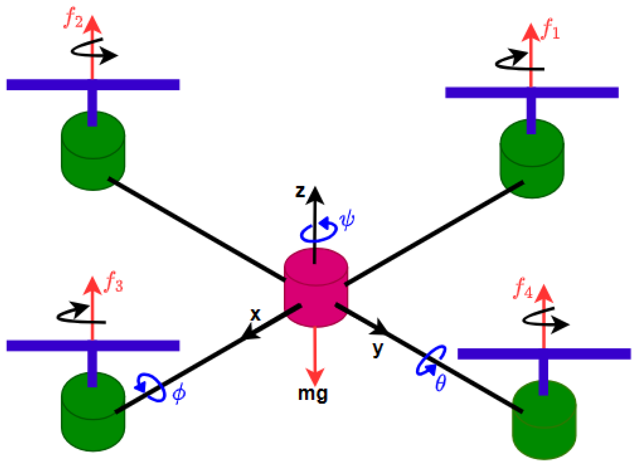
The mechanical structure of the QUAV, as depicted in Figure 1, is relatively simple. It comprises four autonomously controlled rotors affixed to a rigid cross frame. Five forces exert influence on the QUAV: the gravitational force, denoted by $mg$, and the four propeller forces, each labeled $f_i$, which operate along the $z$-axis in the body-fixed reference frame, as illustrated in Figure 1. The indices $i=1,2,3,4$ correspond to the four individual propellers, respectively.

The generation of thrusts and torques on the QUAV involves two sets of identical fixed-pitch propellers. To maintain torque equilibrium, one pair of propellers (1 and 3) rotates clockwise, while the other pair (2 and 4) rotates counterclockwise. Control over the QUAV’s movements is achieved by manipulating the speeds of these independent rotors. Altering the speeds of diametrically opposite rotors induces pitch or roll motion, while yaw motion results from a discrepancy in speed balance between clockwise and counterclockwise rotors. Simultaneous adjustments of these rotor speeds enable vertical motion.

3.1. Mathematical Description

The dynamics of the QUAV have been explored in existing literature. As outlined in [51], when considering small angular velocities, the dynamics of the QUAV can be expressed as follows:

$$\begin{gathered} \ddot{\psi }\left(t\right)=\frac{u_{\psi }\left(t\right)}{I_{zz}}+\frac{\left(I_{xx}-I_{yy}\right)\dot{\varphi }\left(t\right)\dot{\theta }\left(t\right)}{I_{zz}}+\dot{\varphi }\left(t\right)\dot{\theta }\left(t\right), \\ \ddot{\theta }\left(t\right)=\frac{u_{\theta }\left(t\right)}{I_{yy}}+\frac{\left(I_{zz}-I_{xx}\right)\dot{\psi }\left(t\right)\dot{\varphi }\left(t\right)}{I_{yy}}-\dot{\psi }\left(t\right)\dot{\varphi }\left(t\right), \\ \ddot{\varphi }\left(t\right)=\frac{u_{\varphi }\left(t\right)}{I_{xx}}+\frac{\left(I_{yy}-I_{zz}\right)\dot{\psi }\left(t\right)\dot{\theta }\left(t\right)}{I_{xx}}+\dot{\psi }\left(t\right)\dot{\theta }\left(t\right), \\ \ddot{x}\left(t\right)=\left(S\psi \left(t\right)S\varphi \left(t\right)+C\psi \left(t\right)S\theta \left(t\right)C\varphi \left(t\right)\right)\frac{u_z\left(t\right)}{m}, \\ \ddot{y}\left(t\right)=\left(-C\psi \left(t\right)S\varphi \left(t\right)+S\psi \left(t\right)S\theta \left(t\right)C\varphi \left(t\right)\right)\frac{u_z\left(t\right)}{m}, \\ \ddot{z}\left(t\right)=\left(C\theta \left(t\right)C\varphi \left(t\right)\right)\frac{u_z\left(t\right)}{m}-g, \end{gathered}$$

(10)

where, in the horizontal plane, the coordinates $x\left(t\right)$ and $y\left(t\right)$ define the position, while the vertical position is represented by the coordinate $z\left(t\right)$ (see Figure 1), $\psi \left(t\right)$ is the yaw angle around $z$ axis, $\theta \left(t\right)$ is the pitch angle around the $y$ axis, and $\varphi \left(t\right)$ is the roll angle around the $x$ axis. $m$ denotes the mass of the QUAV, $g$ is the acceleration due to gravity, $I_{xx}$, $I_{yy}$, and $I_{zz}$ are the moments of inertia along the $x$, $y$, and $z$ axes, respectively. $C$ and $S$ represent the trigonometric functions cosine and sine, respectively. The control inputs $u_z\left(t\right)$, $u_{\psi }(t)$, $u_{\theta }(t)$, and $u_{\varphi }(t)$ are the total thrust input and the angular yaw, pitch, and roll moments, respectively.

The control inputs of the QUAV model are defined by

$$\left[\begin{array}{c}\begin{array}{c}{u}_z\left(t\right)\\ u_{\psi }\left(t\right)\\ u_{\theta }\left(t\right)\end{array}\\ u_{\varphi }\left(t\right)\end{array}\right]=\left[\begin{array}{cccc}1& 1& 1& 1\\ l& -l& l& -l\\ l& 0& -l& 0\\ 0& l& 0& -l\end{array}\right]\left[\begin{array}{c}\begin{array}{c}{f}_1\left(t\right)\\ f_2\left(t\right)\\ f_3\left(t\right)\end{array}\\ f_4\left(t\right)\end{array}\right]$$

(11)

where $l$ is the distance from the motors to the center of gravity of the QUAV and $f_i$ (with $i=1, 2, 3, 4$) denotes the generated force for each motor of the QUAV.

We use state-space representation since it facilitates the analysis of the system’s stability, controllability, and observability using mathematical tools such as linear algebra and modern control theory used for the design of dynamical observers. Therefore, we transform the QUAV model into the state-space representation. Selecting the state vector as $\mathcal{Z}={\left[x,\dot{x},y,\dot{y},z,\dot{z},\psi ,\dot{\psi },\theta ,\dot{\theta },\varphi ,\dot{\varphi }\right]}^T$, the state-space representation of the QUAV model is given by

$$\dot{\mathcal{Z}}\left(t\right)=\left[\begin{array}{c}\begin{array}{c}{\mathcal{z}}_2\left(t\right)\\ p_1\left(t\right)u_z\left(t\right)/m\\ \begin{array}{c}{\mathcal{z}}_4\left(t\right)\\ p_2\left(t\right)u_z\left(t\right)/m\\ \begin{array}{c}{\mathcal{z}}_6\left(t\right)\\ \left(p_3\left(t\right)u_z\left(t\right)/m\right)-g\\ \begin{array}{c}{\mathcal{z}}_8\left(t\right)\\ a_1{\mathcal{z}}_{10}\left(t\right){\mathcal{z}}_{12}\left(t\right)+{\mathcal{z}}_{10}\left(t\right){\mathcal{z}}_{12}\left(t\right)+b_1{u}_{\psi }\left(t\right)\\ \begin{array}{c}{\mathcal{z}}_{10}\left(t\right)\\ {a_2\mathcal{z}}_8\left(t\right){\mathcal{z}}_{12}\left(t\right)-{\mathcal{z}}_8\left(t\right){\mathcal{z}}_{12}\left(t\right)+b_2{u}_{\theta }\left(t\right)\\ {\mathcal{z}}_{12}\left(t\right)\end{array}\end{array}\end{array}\end{array}\end{array}\\ {a_3\mathcal{z}}_8\left(t\right){\mathcal{z}}_{10}\left(t\right)+{\mathcal{z}}_8\left(t\right){\mathcal{z}}_{10}\left(t\right)+b_3{u}_{\varphi }\left(t\right)\end{array}\right],$$

(12)

where $\mathcal{Z}=\left[x,\dot{x},y,\dot{y},z,\dot{z},\psi ,\dot{\psi },\theta ,\dot{\theta },\varphi ,\dot{\varphi }\right]=\left[{\mathcal{z}}_1,{\mathcal{z}}_2,{\mathcal{z}}_3,{\mathcal{z}}_4,{\mathcal{z}}_5,{\mathcal{z}}_6,{\mathcal{z}}_7,{\mathcal{z}}_8,{\mathcal{z}}_9,{\mathcal{z}}_{10},{\mathcal{z}}_{11},{\mathcal{z}}_{12}\right]\in {\mathbb{R}}^{12}$ is the state vector, and the parameters of the model are defined as follows

$$\begin{gathered} a_1=\left(\right(I_{xx}-I_{yy}\left)\right)/I_{zz}, \\ {a}_2=\left(\left(I_{zz}-I_{xx}\right)\right)/I_{yy,} \\ {a}_3=\left(\left(I_{yy}-I_{zz}\right)\right)/I_{xx}, \\ {b}_1=1/I_{zz}, \\ {b}_2=1/I_{yy}, \\ {b}_3=1/I_{xx}, \\ {p}_1\left(t\right)=S{\mathcal{z}}_7\left(t\right)S{\mathcal{z}}_{11}\left(t\right)+C{\mathcal{z}}_7\left(t\right)S{\mathcal{z}}_9\left(t\right)C{\mathcal{z}}_{11}\left(t\right), \\ {p}_2\left(t\right)=-C{\mathcal{z}}_7\left(t\right)S{\mathcal{z}}_{11}\left(t\right)+S{\mathcal{z}}_7\left(t\right)S{\mathcal{z}}_9\left(t\right)C{\mathcal{z}}_{11}\left(t\right), \\ {p}_3\left(t\right)=C{\mathcal{z}}_9\left(t\right)C{\mathcal{z}}_{11}\left(t\right). \end{gathered}$$

(13)

The nonlinear dynamic model of the QUAV represented by Equation (12) is transformed into a linear-time invariant model through a linearized process around the equilibrium point of the QUAV. The QUAV has a main operating point, which corresponds to the point where the QUAV is fixed at coordinates $x, y, z$. This operating point occurs when the acceleration on the $z$ axis and the angles of the QUAV are zero, corresponding to an equilibrium point $\left(\varphi ,\theta ,\psi ,\ddot{z}\right)=(\mathrm{0,0},\mathrm{0,0})$ [41]. The resulting linear model is expressed in state-space form:

$$\begin{gathered} \dot{\mathcal{Z}}\left(t\right)=\mathcal{A}\mathcal{Z}\left(t\right)+\mathcal{B}\mathcal{U}\left(t\right), \\ \mathcal{Y}\left(t\right)=\mathcal{H}\mathcal{Z}\left(t\right), \end{gathered}$$

(14)

where the system matrix $\mathcal{A}$, and the input matrix $\mathcal{B}$, are defined as

$$\begin{gathered} \mathcal{A}=\left[ \begin{array}{cccccccccccc}0& 1& 0& 0& 0& 0& 0& 0& 0& 0& 0& 0\\ 0& 0& 0& 0& 0& 0& 0& 0& g& 0& 0& 0\\ 0& 0& 0& 1& 0& 0& 0& 0& 0& 0& 0& 0\\ 0& 0& 0& 0& 0& 0& 0& 0& 0& 0& -g& 0\\ 0& 0& 0& 0& 0& 1& 0& 0& 0& 0& 0& 0\\ 0& 0& 0& 0& 0& 0& 0& 0& 0& 0& 0& 0\\ 0& 0& 0& 0& 0& 0& 0& 1& 0& 0& 0& 0\\ 0& 0& 0& 0& 0& 0& 0& 0& 0& 0& 0& 0\\ 0& 0& 0& 0& 0& 0& 0& 0& 0& 1& 0& 0\\ 0& 0& 0& 0& 0& 0& 0& 0& 0& 0& 0& 0\\ 0& 0& 0& 0& 0& 0& 0& 0& 0& 0& 0& 1\\ 0& 0& 0& 0& 0& 0& 0& 0& 0& 0& 0& 0\end{array} \right], \\ \mathcal{B}=\left[\begin{array}{cccc}0& 0& 0& 0\\ 0& 0& 0& 0\\ 0& 0& 0& 0\\ 0& 0& 0& 0\\ 0& 0& 0& 0\\ 1/m& 0& 0& 0\\ 0& 0& 0& 0\\ 0& 0& 0& 1/I_{zz}\\ 0& 0& 0& 0\\ 0& 0& 1/I_{yy}& 0\\ 0& 0& 0& 0\\ 0& 1/I_{xx}& 0& 0\end{array}\right], \end{gathered}$$

(15)

respectively, and assuming $\mathcal{Y}={\left[x \dot{x} y \dot{y} z \dot{z} \psi \dot{\psi } \theta \dot{\theta } \varphi \dot{\varphi }\right]}^T$ as the system output vector, it follows that the output matrix is given by

$$\mathcal{H}=\left[ \begin{array}{cccccccccccc}1& 0& 0& 0& 0& 0& 0& 0& 0& 0& 0& 0\\ 0& 1& 0& 0& 0& 0& 0& 0& 0& 0& 0& 0\\ 0& 0& 1& 0& 0& 0& 0& 0& 0& 0& 0& 0\\ 0& 0& 0& 1& 0& 0& 0& 0& 0& 0& 0& 0\\ 0& 0& 0& 0& 1& 0& 0& 0& 0& 0& 0& 0\\ 0& 0& 0& 0& 0& 1& 0& 0& 0& 0& 0& 0\\ 0& 0& 0& 0& 0& 0& 1& 0& 0& 0& 0& 0\\ 0& 0& 0& 0& 0& 0& 0& 1& 0& 0& 0& 0\\ 0& 0& 0& 0& 0& 0& 0& 0& 1& 0& 0& 0\\ 0& 0& 0& 0& 0& 0& 0& 0& 0& 1& 0& 0\\ 0& 0& 0& 0& 0& 0& 0& 0& 0& 0& 1& 0\\ 0& 0& 0& 0& 0& 0& 0& 0& 0& 0& 0& 1\end{array} \right].$$

(16)

3.2. Control of the Quadrotor Unmanned Aerial Vehicle (QUAV)

Due to the dynamic instability of the QUAV, a control algorithm is required to stabilize it. Hence, this section is dedicated to the development of a control strategy aimed at stabilizing the QUAV at its origin. Specifically, we introduce an optimal control strategy designed to regulate the QUAV’s position at the origin.

The adoption of an optimal regulator control strategy over alternative methods, such as sliding mode control, for addressing the regulation challenges of the QUAV is driven by several crucial factors. Primarily, a structured and mathematically rigorous approach is provided by optimal regulator control methodologies for developing controllers that minimize predetermined cost functions while adhering to system constraints. This framework enables the customization of control strategies to meet specific performance goals and operational needs, including considerations for energy efficiency. Furthermore, the integration of complex dynamics and constraints inherent to QUAVs, such as actuator saturation and state constraints, is enabled by optimal regulator control. This ensures that operational boundaries are maintained within safe operational limits while overall performance is optimized. Additionally, flexibility in selecting cost functions and optimization criteria is offered by optimal regulator control techniques, allowing for the prioritization of various performance metrics based on the specific demands of the application [52]. This adaptability is particularly advantageous in the realm of QUAVs, where a range of control strategies may be required due to diverse mission objectives and environmental conditions.

For the optimal regulator design, we consider the multi-input, multi-output dynamic system described by

$$\begin{gathered} \dot{\mathcal{Z}}\left(t\right)=\mathcal{A}\mathcal{Z}\left(t\right)+\mathcal{B}\mathcal{U}\left(t\right), \\ \mathcal{Y}\left(t\right)=\mathcal{H}\mathcal{Z}\left(t\right), \end{gathered}$$

(17)

and we design a linear quadratic regulator (LQR) law as

$$\mathcal{U}\left(t\right)=-K\mathcal{Z}\left(t\right),$$

(18)

to minimize the performance index

$$J={\int }_0^{\infty }({\mathcal{Z}}^T(t)Q\mathcal{Z}(t)+{\mathcal{U}}^T(t)R\mathcal{U}(t))dt,$$

(19)

where $Q$, and $R$ are positive-definite real symmetric matrices. It is important to note that if the unknown elements of the matrix $K$ are determined to minimize the performance index given by Equation (19), then the control law $\mathcal{U}\left(t\right)$ is optimal for any initial state $\mathcal{Z}\left(0\right)$. The $Q$, and $R$ matrices serve as weighting matrices for the state variables and the input variables, respectively. The first term of the control law penalizes the error of the state variables, while the second term takes into account the expenditure of energy of the control signals. To solve the optimization problem, we proceed as follows:

• We select the matrices Q and R. To limit the magnitude of the state variables, we penalize states by defining the weight matrix Q as follows:

  $$Q=\left[ \begin{array}{cccccccccccc}10& 0& 0& 0& 0& 0& 0& 0& 0& 0& 0& 0\\ 0& 1& 0& 0& 0& 0& 0& 0& 0& 0& 0& 0\\ 0& 0& 1& 0& 0& 0& 0& 0& 0& 0& 0& 0\\ 0& 0& 0& 1& 0& 0& 0& 0& 0& 0& 0& 0\\ 0& 0& 0& 0& 1& 0& 0& 0& 0& 0& 0& 0\\ 0& 0& 0& 0& 0& 1& 0& 0& 0& 0& 0& 0\\ 0& 0& 0& 0& 0& 0& 1& 0& 0& 0& 0& 0\\ 0& 0& 0& 0& 0& 0& 0& 1& 0& 0& 0& 0\\ 0& 0& 0& 0& 0& 0& 0& 0& 1& 0& 0& 0\\ 0& 0& 0& 0& 0& 0& 0& 0& 0& 50& 0& 0\\ 0& 0& 0& 0& 0& 0& 0& 0& 0& 0& 1& 0\\ 0& 0& 0& 0& 0& 0& 0& 0& 0& 0& 0& 1\end{array} \right],$$

  (20)

  and equal penalties are applied to each control input by selecting the weighting matrix $R$ as an identity matrix, as follows:

  $$R=\left[\begin{array}{c}\begin{array}{c}\begin{array}{ccc}1& 0& \begin{array}{cc}0& 0\end{array}\end{array}\\ \begin{array}{ccc}0& 1& \begin{array}{cc}0& 0\end{array}\end{array}\end{array}\\ \begin{array}{c}\begin{array}{ccc}0& 0& \begin{array}{cc}1& 0\end{array}\end{array}\\ \begin{array}{ccc}0& 0& \begin{array}{cc}0& 1\end{array}\end{array}\end{array}\end{array}\right].$$

  (21)

The choice of $Q$ and $R$ matrices depends on the specific requirements and objectives of the control problem. It often involves a trade-off between achieving desired performance and minimizing control effort. The selection process may involve system identification, optimization techniques, tuning methods, and, in this particular case, heuristics based on experience and domain knowledge. In the $Q$ matrix, the first and tenth components of the QUAV state are penalized more than other components to reduce the error to less than 5. Meanwhile, the matrix $R$ was selected as an identity matrix to apply equal penalties to each control input.

2.

We solve the reduced-matrix Riccati equation given by

$${\mathcal{A}}^{T}P+P\mathcal{A}-P\mathcal{B}{R}^{-1}{\mathcal{B}}^{T}P+Q=0$$

(22)

for the matrix $P$. Since more than one matrix $P$ may satisfy the Riccati equation, we select one that is a positive-definite matrix.

3.

We find the feedback gain matrix solving the equation K = −R⁻¹B^TP. Thus, the resulting gain matrix that stabilizes the QUAV system is given by

$$K=\left[\begin{array}{cccccccccccc}0& 0& 0& 0& 1& 1.95& 0& 0& 0& 0& 0& 0\\ 0& 0& -1& -1.46& 0& 0& 0& 0& 0& 0& 5.59& 1.07\\ 3.16& 4.04& 0& 0& 0& 0& 0& 0& 23.74& 7.11& 0& 0\\ 0& 0& 0& 0& 0& 0& 1& 1.03& 0& 0& 0& 0\end{array}\right]$$

(23)

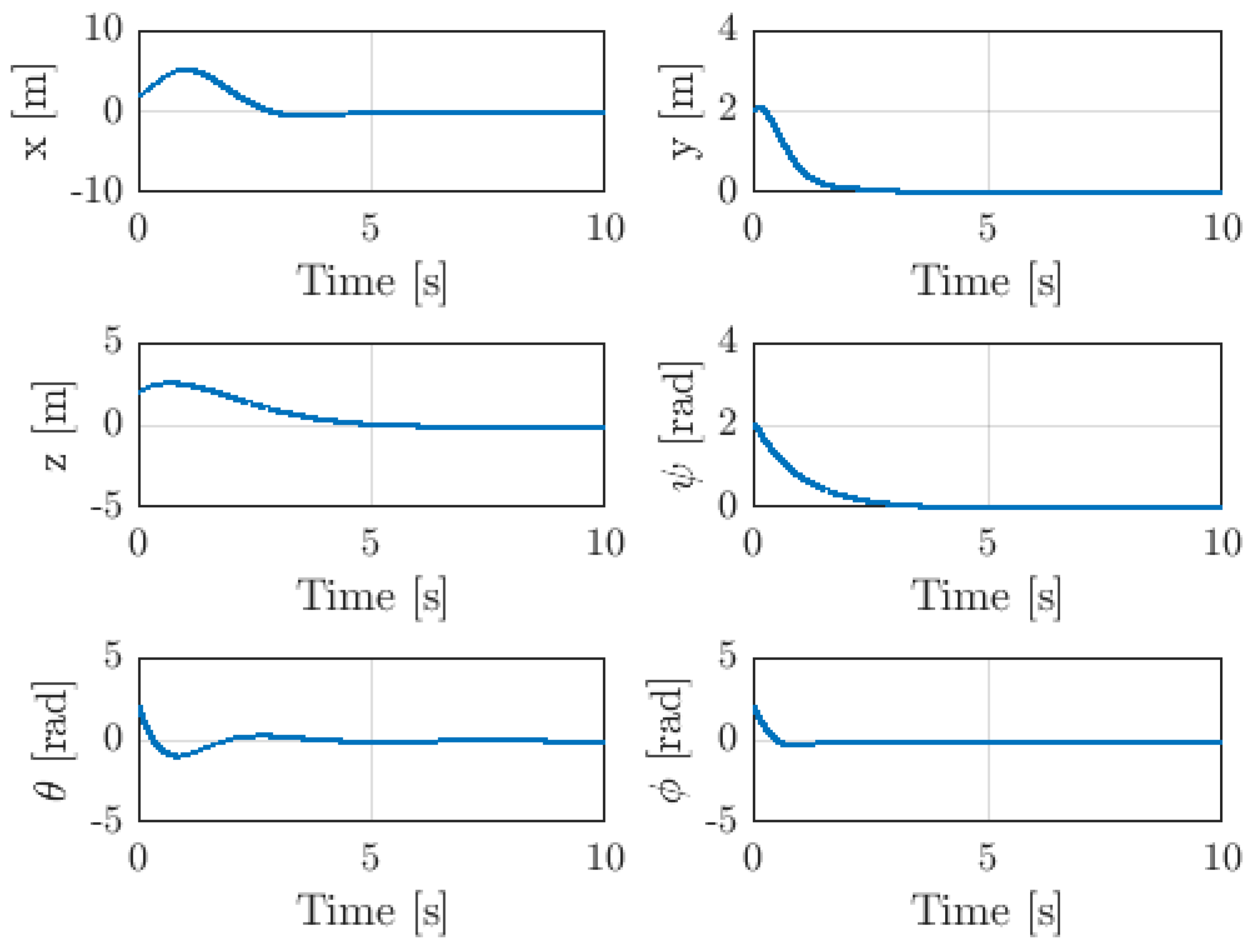
Since all the closed-loop eigenvalues of $\mathcal{A}-K\mathcal{B}$ are in the left half-complex plane, the closed-loop system is asymptotically stable. To verify this assumption, we simulate the closed-loop system subject to the initial conditions $\mathcal{Z}=\left[2, 2, 2, 2, 2, 2, 2, 2, 2, 2, 2, 2\right]\in {\mathbb{R}}^{12}$, and the operation parameters shown in

Table 1. Parameters of the QUAV system [41].

Parameter	Symbol	Value
Mass	m	1.4 kg
Arm length	l	1 m
Moment of Inertia along the x-axis	Ixx	0.0116 kg m2
Moment of Inertia along the y-axis	Iyy	0.0116 kg m2
Moment of Inertia along the z-axis	Izz	0.0232 kg m2

. These parameters were obtained from [41]. Figure 2 shows the simulation results of using the linear quadratic regulator (LQR). It demonstrates how the positions (x, y, z), and the orientations (ψ, θ, ϕ) converge to zero.

3.3. Actuator Faults in the Quadrotor Unmanned Aerial Vehicle (QUAV)

The propulsion system of a QUAV consists of four identical brushless motors paired with fixed-pitched propellers, illustrated in Figure 1. Therefore, the QUAVs heavily depend on precise control of their four rotors to maintain stability, maneuverability, and overall operational efficiency. Actuator faults, ranging from motor deterioration to sudden malfunctions or partial failures in the propulsion system, can significantly disrupt the QUAV’s flight dynamics and compromise its mission objectives, therefore diminishing its reliability and safety. The effects of actuator faults in QUAVs go beyond just making them perform worse; they can also put the vehicle’s safety at risk, along with nearby buildings and people. Consequently, research and development efforts have increasingly focused on understanding, modeling, and mitigating actuator faults in QUAVs to bolster the reliability and resilience of these aerial vehicles [53].

In this research, we adopt an approach where actuator faults are conceptualized as additional signals occurring within the input channel of the QUAV system. By viewing actuator faults in this manner, we aim to distinguish this fault. To achieve this, we propose an observer-based method for estimating these faults. Through analysis and simulation, we explore the implications of incorporating such fault models into QUAV dynamics.

The actuator fault considered in this paper refers to a partial loss of control effectiveness, which is recognized as one of the most common actuator faults. We modeled this fault as a time-variant sinusoidal signal given by

$$\mathcal{F}\left(t\right)=M\mathit{sin}\left(\omega t\right),$$

(24)

where $M$, and $\omega$ are the amplitude and the frequency of the actuator fault, respectively. We assume that this fault acts additively. Therefore, the actuator fault is modeled as

$$u_i^f(t)=u_i(t)+{\mu }_i\mathcal{F}\left(t\right),$$

(25)

where $u_i^f(t)$ denotes the $i$th component of the input control vector $\mathcal{U}\left(t\right)$. A value of ${\mu }_i=0$ indicates that the $i$th actuator is functioning normally, while a value of ${\mu }_i>0$ indicates a loss of control effectiveness in the $i$-th actuator.

Therefore, the dynamics model of the QUAV considering actuator faults can be written as

$$\dot{\mathcal{Z}}\left(t\right)=\mathcal{A}\mathcal{Z}\left(t\right)+\mathcal{B}\mathcal{U}\left(t\right)+\mathcal{D}\mathcal{F}\left(t\right),$$

(26)

where the term $\mathcal{D}\mathcal{F}\left(t\right)$ denotes the addition of an actuator fault, and the matrix $\mathcal{D}=\mathcal{B}{\rm M}$, with ${\rm M}={\left[{\mu }_1 {\mu }_2 {\mu }_3 {\mu }_4\right]}^T$ is a fault-coupling matrix.

4. Actuator Fault Estimation Using Dynamical Observers

In QUAV systems, ensuring the accurate and reliable performance of actuators is pivotal for the overall functionality of the aircraft. Nevertheless, actuator faults, such as degradation or unexpected damage, can significantly impact the system’s behavior, potentially leading to a QUAV crash. To avoid these issues, it is important to detect and isolate these faults as quickly as possible [54].

The actuator fault detection and isolation (FDI) problem involves the timely identification of deviations from normal system behavior and the accurate identification of the faulty components responsible for these deviations [55]. Over the last few decades, the application of dynamical observers (also known as observers or estimators) for fault detection and isolation problems has garnered significant attention. This attention is owed to their ability to provide early and accurate fault detection, adapt to diverse system dynamics, and remain compatible with nonlinear and complex systems [56].

Traditionally, the concept of residual generation is employed to solve the fault detection and isolation problem using observers. Residuals are computed by measuring the difference between the system output and the output predicted by the observer. Under normal operational conditions, the residual is expected to be negligible; however, in the presence of faults, it is anticipated to show a significant deviation from zero. By analyzing these residuals, one can detect and isolate faults in a system [57]. However, because residual-based approaches rely heavily on an accurate model of the system, any discrepancies between the model and the actual system behavior can lead to false alarms or missed detections [58].

In recent decades, there has been a growing interest in employing observers to address FDI problems, obviating the need for residual generators. This methodology, known as the fault estimation approach, seeks to directly quantify or infer the magnitude and characteristics of faults within a system [59]. Over the past two decades, sliding mode observers (SMOs) have emerged as valuable tools for fault estimation in dynamic systems due to their robustness and simplicity. Leveraging the sliding mode control principle, SMOs facilitate the estimation of system states and fault signals, even in the presence of uncertainties and disturbances [60]. A key advantage of SMOs lies in their capacity to operate without explicit knowledge of system dynamics, rendering them suitable for diverse applications where accurate system models may be elusive or impractical to obtain. Moreover, SMOs offer robust performance in the face of modeling errors and disturbances, therefore enhancing their efficacy in tasks related to fault detection and estimation, particularly within the domain of QUAVs [61].

4.1. Actuator Fault Estimation Using a Sliding Mode Observer (SMO)

A sliding mode observer (SMO) is essentially a mathematical model of a system driven by its inputs and measured outputs, as well as the output estimation error. The output estimation error is injected into the SMO as a corrective term through a nonlinear switching function (referred to as the nonlinear output estimation error) to force the observer states to converge to the system states. When this occurs, it is said that a sliding motion takes place. During the sliding motion, the low-frequency component of the nonlinear output estimation error (known as equivalent output error injection) contains information about actuator faults acting in the input channel of the system. By suitably filtering the equivalent output error injection, an accurate estimate of the actuator faults can be obtained [62].

The design of the SMO is based on a linear system subject to actuator faults given by

$$\begin{gathered} \dot{\mathcal{X}}\left(t\right)=\mathcal{A}\mathcal{X}\left(t\right)+\mathcal{B}\mathcal{U}\left(t\right)+\mathcal{D}\mathcal{F}\left(t\right), \\ \mathcal{Y}\left(t\right)=\mathcal{H}\mathcal{X}\left(t\right), \end{gathered}$$

(27)

where $\mathcal{X}\left(t\right)\in {\mathbb{R}}^n$ is the state vector, $\mathcal{Y}\left(\mathrm{t}\right)\in {\mathbb{R}}^{\mathrm{p}}$ is the output vector, and $\mathcal{U}\left(t\right)\in {\mathbb{R}}^m$ is the input vector. $\mathcal{A}\in {\mathbb{R}}^{n\times n}$ is the system matrix, $\mathcal{B}{\in \mathbb{R}}^{n\times m}$ is the input matrix, $\mathcal{H}\in {\mathbb{R}}^{p\times n}$ is the output matrix, and $\mathcal{D}\in {\mathbb{R}}^{n\times q}$ is the fault-coupling matrix. To design an SMO for the system described by Equation (27), it is necessary for matrices $\mathcal{B},\mathcal{H}$, and $\mathcal{D}$ to be full rank and for the function $\mathcal{F}:{\mathbb{R}}_{+}\to {\mathbb{R}}^q$, which represents an actuator fault, to be bounded such that $‖\mathcal{F}\left(t\right)‖\le \rho$, where $\rho \in {\mathbb{R}}_{+}$. Hence $‖\mathcal{F}\left(t\right)‖$ denotes the Euclidian norm. Furthermore, we presume that the system outputs are being measured. We also assume that the dynamical system adheres to the following two conditions: $rank\left(HD\right)=q$, and the invariant zeros of the triple ($\mathcal{A}$, $\mathcal{B}$, $\mathcal{H}$) must lie in $C^{-}$ (left half-complex plane).

Given the conditions stated above, it is possible to find a linear transformation $T$ that allows for the reformulation of the system model in Equation (27). This transformation enables a new representation of the system, facilitating further analysis and observer design. In this new coordinate system, the system, input, coupling fault, and output matrices are given as follows:

$$T\mathcal{A}{T}^{-1}=\left[\begin{array}{cc}{\mathcal{A}}_{11}& {\mathcal{A}}_{12}\\ {\mathcal{A}}_{21}& {\mathcal{A}}_{22}\end{array}\right], T\mathcal{B}=\left[\begin{array}{c}{\mathcal{B}}_1\\ {\mathcal{B}}_2\end{array}\right], T\mathcal{D}=\left[\begin{array}{c}0\\ {\mathcal{D}}_2\end{array}\right], and \mathcal{H}{T}^{-1}=\left[\begin{array}{cc}0& I_p\end{array}\right],$$

(28)

respectively. Where ${\mathcal{A}}_{11}\in {\mathbb{R}}^{\left(n-p\right)\times \left(n-p\right)}$, ${\mathcal{A}}_{12}\in {\mathbb{R}}^{\left(n-p\right)\times p}$, ${\mathcal{A}}_{21}\in {\mathbb{R}}^{p\times \left(n-p\right)}$, ${\mathcal{A}}_{22}\in {\mathbb{R}}^{p\times p}$, ${\mathcal{B}}_1\in {\mathbb{R}}^{\left(n-p\right)\times m}, {\mathcal{B}}_2\in {\mathbb{R}}^{p\times m}$, ${ D}_2\in {\mathbb{R}}^{p\times q}$, and $I_p\in {\mathbb{R}}^{p\times p}$ represents the identity matrix. Thus, the dynamical model of the new system can be written as

$$\begin{gathered} {\dot{\mathcal{X}}}_1(t)={\mathcal{A}}_{11}{\mathcal{X}}_1\left(t\right)+{\mathcal{A}}_{12}{\mathcal{X}}_2\left(t\right)+{\mathcal{B}}_1\mathcal{U}\left(t\right), \\ {\dot{\mathcal{X}}}_2(t)={\mathcal{A}}_{21}{\mathcal{X}}_1(t)+{\mathcal{A}}_{22}{\mathcal{X}}_2(t)+{\mathcal{B}}_2\mathcal{U}\left(t\right)+{\mathcal{D}}_2\mathcal{F}\left(t\right), \\ \mathcal{Y}(t)={\mathcal{X}}_2\left(t\right), \end{gathered}$$

(29)

where ${\mathcal{X}}_1\left(t\right)\in {\mathbb{R}}^{n-p}$ represents the vector of unmeasured states, ${\mathcal{X}}_2\left(\mathrm{t}\right)\in {\mathbb{R}}^{\mathrm{p}}$ represents the vector of measured states, and the matrix ${\mathcal{A}}_{11}$ has stable eigenvalues. The transformed system model outlined by Equation (29) will serve as the basis for designing the SMO. The observer structure under consideration can be succinctly represented as

$$\begin{gathered} \dot{{\widehat{\mathcal{X}}}_1}(t)={\mathcal{A}}_{11}{\widehat{\mathcal{X}}}_1\left(t\right)+{\mathcal{A}}_{12}{\widehat{\mathcal{X}}}_2\left(t\right)+{\mathcal{B}}_1\mathcal{U}\left(t\right)-{\mathcal{A}}_{12}{E}_y(t), \\ \dot{{\widehat{\mathcal{X}}}_2}(t)={\mathcal{A}}_{21}{\widehat{\mathcal{X}}}_1(t)+{\mathcal{A}}_{22}{\widehat{\mathcal{X}}}_2(t)+{\mathcal{B}}_2\mathcal{U}\left(t\right)-\left({\mathcal{A}}_{22}-{\mathcal{A}}_{22}^s\right)E_y(t)+{\mathcal{V}}_2(t). \end{gathered}$$

(30)

where ${\widehat{\mathcal{X}}}_1\left(t\right)$ and ${\widehat{\mathcal{X}}}_2\left(t\right)$ represent the state estimates for ${\mathcal{X}}_1\left(t\right)$ and ${\mathcal{X}}_2\left(t\right)$, respectively. $E_y\left(t\right)$ denotes the error between the estimates and the true outputs of the system, ${\mathcal{A}}_{22}^s$ denotes a stable design matrix, and the discontinuous signal ${\mathcal{V}}_2\left(t\right)\in {\mathbb{R}}^p$, is expressed as

$${\mathcal{V}}_2(t)=\left\{\begin{array}{c}-\rho ‖D_2‖\frac{Q_2{E}_y\left(t\right)}{‖Q_2{E}_y\left(t\right)‖} \mathrm{if} E_y(t)\ne 0\\ 0 \mathrm{otherwise},\end{array}\right.$$

(31)

where $Q_2\in {\mathbb{R}}^{p\times p}$ is a symmetric positive-definite Lyapunov matrix for ${\mathcal{A}}_{22}^s$, ${ D}_2\in {\mathbb{R}}^{p\times q}$ is the transformed fault-coupling matrix, $E_y$(t) is the output estimation error vector, and $\rho$ is a design parameter. To achieve adequate fault estimation, the value of $\rho$ should be selected to satisfy $\rho >‖\mathcal{F}\left(t\right)‖$. However, it should not be chosen that is much larger than the magnitude of the fault, as this increases the chattering.

The state estimation error vector of the unmeasured states $E_1\left(t\right)$, is defined as the difference between the estimated state vector ${\widehat{\mathcal{X}}}_1\left(t\right)$ and the actual state vector ${\mathcal{X}}_1\left(t\right)$. Similarly, the output estimation error vector $E_y\left(t\right)$, is defined as the difference between the estimated output vector ${\widehat{\mathcal{X}}}_2\left(t\right)$ and the actual output vector ${\mathcal{X}}_2\left(t\right)$. Thus, the dynamics of the error are expressed as

$$\begin{gathered} {\dot{E}}_1\left(t\right)={\mathcal{A}}_{11}{E}_1\left(t\right) \\ { \dot{E}}_y\left(t\right)={\mathcal{A}}_{21}{E}_1\left(t\right)+{\mathcal{A}}_{22}^s{E}_y\left(t\right)+{\mathcal{V}}_2\left(t\right)-{\mathcal{D}}_2\mathcal{F}\left(t\right) \end{gathered}$$

(32)

To establish the stability of the proposed observer, our objective is to demonstrate the asymptotic convergence of both $E_y\left(t\right)$ and ${\dot{E}}_y(t)$ to zero as the error dynamics attain sliding motion within a finite time frame. This endeavor is accomplished through the application of the Lyapunov approach, which provides a rigorous framework for analyzing the system’s stability properties.

Proposition 1.

A family of symmetric positive-definite matrices Q₂ exists, ensuring the asymptotic stability of the dynamical error system depicted in Equation (32).

Proof. 

Let $W_1\in {\mathbb{R}}^{(n-p)\times (n-p)}$ and $W_2\in {\mathbb{R}}^{p\times p}$ denote symmetric positive-definite design matrices. We define $Q_2\in {\mathbb{R}}^{p\times p}$ as the unique symmetric positive-definite solution to the Lyapunov equation

$$Q_2{A}_{22}^s+{\left(A_{22}^{\mathrm{s}}\right)}^T{Q}_2=-W_2,$$

(33)

utilizing the computed value of $Q_2$, we establish the definition of a matrix $\widehat{W}$ as follows:

$$\widehat{W}=A_{21}^T{Q}_2{W}_2^{-1}{Q}_2{A}_{21}+W_1,$$

(34)

where $\widehat{W}={\widehat{W}}^T>0$ (i.e., it is a positive-definite matrix). Let $Q_1\in {\mathbb{R}}^{(n-p)\times (n-p)}$ be the unique symmetric positive-definite solution to the Lyapunov equation

$$Q_1{A}_{11}+A_{11}^T{Q}_1=-\widehat{W}.$$

(35)

Consider as a candidate Lyapunov function the function given by

$$V\left(t\right)=E_1^T\left(t\right)Q_1{E}_1\left(t\right)+E_y^T\left(t\right)Q_2{E}_y\left(t\right).$$

(36)

The derivative of the candidate Lyapunov function yields

$$\dot{V}\left(t\right)={\dot{E}}_1^T\left(t\right)Q_1{E}_1\left(t\right)+E_1^T\left(t\right)Q_1{\dot{E}}_1\left(t\right)+{\dot{E}}_y^T\left(t\right)Q_2{E}_y\left(t\right)+E_y^T\left(t\right)Q_2{\dot{E}}_y\left(t\right),$$

(37)

where

$${\dot{E}}_1^T\left(t\right)Q_1{E}_1\left(t\right)+E_1^T\left(t\right)Q_1{\dot{E}}_1\left(t\right)=-E_1^T\left(t\right)\widehat{W}{E}_1\left(t\right),$$

(38)

and

$$\begin{gathered} {\dot{E}}_y^T\left(t\right)Q_2{E}_y\left(t\right)+E_y^T\left(t\right)Q_2{\dot{E}}_y\left(t\right)\hspace{1em}\hspace{1em}\hspace{1em}\hspace{1em}\hspace{1em}\hspace{1em}\hspace{1em}\hspace{1em}\hspace{1em}\hspace{1em} \\ \hspace{1em}\hspace{1em}\hspace{1em}\hspace{1em}\hspace{1em}\hspace{1em}\hspace{1em}\hspace{1em}\hspace{1em}\hspace{1em}\hspace{1em}\hspace{1em}=E_1^T\left(t\right)A_{21}^T{Q}_2{E}_y\left(t\right)+E_y^T\left(t\right)Q_2{A}_{21}{E}_1\left(t\right)-E_y^T\left(t\right)W_2{E}_y\left(t\right) \\ \hspace{1em}\hspace{1em}\hspace{1em}\hspace{1em}\hspace{1em}+2E_y^T\left(t\right)Q_2{\mathcal{V}}_2\left(t\right)-2E_y^T\left(t\right)Q_2{D}_2\mathcal{F}\left(t\right). \end{gathered}$$

(39)

Defining ${\overline{E}}_y(t)=E_y(t)-W_2^{-1}{Q}_2{A}_{21}{E}_1(t)$, then Equation (39) can be rewritten as

$$\begin{array}{cc}{\dot{E}}_y^T\left(t\right)Q_2{E}_y\left(t\right)+& E_y^T\left(t\right)Q_2{\dot{E}}_y\left(t\right)\hfill \\ & =-{\overline{E}}_y^T\left(t\right)W_2{\overline{E}}_y\left(t\right)+E_1^T\left(t\right)A_{21}^T{Q}_2{W}_2^{-1}{Q}_2{A}_{21}{E}_1\left(t\right)+2E_y^T\left(t\right)Q_2{\mathcal{V}}_2\left(t\right)\\ & -2E_y^T{Q}_2{D}_2\mathcal{F}\left(t\right).\hfill \end{array}$$

(40)

Therefore, the derivative of the candidate Lyapunov function can be rewritten as follows:

$$\begin{array}{c}\hfill \dot{V}\left(t\right)=-E_1^T\left(t\right)\widehat{W}{E}_1\left(t\right)-{\overline{E}}_y^T\left(t\right)W_2{\overline{E}}_y\left(t\right)+E_1^T\left(t\right)A_{21}^T{Q}_2{W}_2^{-1}{Q}_2{A}_{21}{E}_1\left(t\right)\hfill \\ \hspace{1em}\hspace{1em}\hspace{1em}\hspace{1em}\hspace{1em}\hspace{1em}\hspace{1em}+2E_y^T\left(t\right)Q_2{\mathcal{V}}_2\left(t\right)-2E_y^T{Q}_2{D}_2\mathcal{F}\left(t\right)\hfill \\ \hspace{1em}\hspace{1em}\hspace{1em}\hspace{1em}\hspace{1em}\hspace{1em}\hspace{1em}=-E_1^T\left(t\right)W_1{E}_1\left(t\right)-{\overline{E}}_y^T\left(t\right)W_2{\overline{E}}_y\left(t\right)+2E_y^T\left(t\right)Q_2{\mathcal{V}}_2\left(t\right)\hfill \\ \hspace{1em}\hspace{1em}\hspace{1em}\hspace{1em}\hspace{1em}\hspace{1em}\hspace{1em}-2E_y^T\left(t\right)Q_2{D}_2\mathcal{F}\left(t\right)\hfill \\ \hspace{1em}\hspace{1em}\hspace{1em}\hspace{1em}\hspace{1em}\hspace{1em}\hspace{1em}=-E_1^T\left(t\right)W_1{E}_1\left(t\right)-{\overline{E}}_y^T\left(t\right)W_2{\overline{E}}_y\left(t\right)-2\rho ‖D_2‖‖Q_2{E}_y\left(t\right)‖\hfill \\ \hspace{1em}\hspace{1em}\hspace{1em}\hspace{1em}\hspace{1em}\hspace{1em}\hspace{1em}-2E_y^T\left(t\right)Q_2{D}_2\mathcal{F}\left(t\right)\hfill \end{array}$$

(41)

Using the fact that $‖\mathcal{F}\left(\mathrm{t}\right)‖\le \rho$, with $\rho \in {\mathbb{R}}_{+}$, we obtain

$$\begin{array}{c}\hfill \dot{V}\left(t\right)\le -E_1^T\left(t\right)W_1{E}_1\left(t\right)-{\overline{E}}_y^T\left(t\right)W_2{\overline{E}}_y\left(t\right)-2\rho ‖D_2‖‖Q_2{E}_y\left(t\right)‖\hfill \\ \hspace{1em}\hspace{1em}\hspace{1em}\hspace{1em}\hspace{1em}\hspace{1em}\hspace{1em}\hspace{1em}\hspace{1em}+2\rho ‖D_2‖‖Q_2{E}_y\left(t\right)‖=-E_1^T\left(t\right)W_1{E}_1\left(t\right)-{\overline{E}}_y^T\left(t\right)W_2{\overline{E}}_y\left(t\right)\hfill \\ \hspace{1em}\hspace{1em}\hspace{1em}\hspace{1em}\hspace{1em}\hspace{1em}\hspace{1em}\hspace{1em}\hspace{1em}<0,\forall \left(E_1\left(t\right),E_y\left(t\right)\right)\ne 0,\hfill \end{array}$$

(42)

therefore, if the actuator fault satisfies $‖\mathcal{F}\left(\mathrm{t}\right)‖\le \rho$, then the Lyapunov derivative is always negative, and the stability of the observer is proved. □

In the above analysis, it is demonstrated that the error dynamics described by Equation (32) exhibit quadratic stability. This stability property implies that both $E_y(t)$, and ${\dot{E}}_y(t)$ converge to zero asymptotically as the error dynamics achieve sliding motion within a finite time frame.

The observer provided in Equation (30) can be expressed more conveniently in the original coordinates of the system as follows:

$$\begin{gathered} \dot{\widehat{\mathcal{X}}}=\mathcal{A}\widehat{\mathcal{X}}\left(t\right)+\mathcal{B}\mathcal{U}\left(t\right)-G_l{E}_y\left(t\right)+G_{nl}\mathcal{V}\left(t\right) \\ \widehat{\mathcal{Y}}(t)=\mathcal{H}\widehat{\mathcal{X}}(t) \end{gathered}$$

(43)

where $G_l$, and $G_{nl}$ are the linear and nonlinear gain matrices given by

$$\begin{gathered} G_l=T^{-1}\left[\begin{array}{c}{\mathcal{A}}_{12}\\ {\mathcal{A}}_{22}-{\mathcal{A}}_{22}^s\end{array}\right], \\ {G}_{nl}=‖{\mathcal{D}}_2‖T^{-1}\left[\begin{array}{c}0\\ I_p\end{array}\right], \end{gathered}$$

(44)

respectively, and $\mathcal{V}\left(t\right)$ is the output estimation error injection term, which is a nonlinear discontinuous signal defined as

$$\mathcal{V}\left(t\right)=\left[\begin{array}{c}0\\ {\mathcal{V}}_2\left(t\right)\end{array}\right].$$

(45)

To tackle the actuator fault estimation issue employing an SMO, we leverage its robustness properties. Upon achieving sliding motion, both $E_y\left(t\right)=0$ and ${\dot{E}}_y\left(t\right)=0$ are forced to zero in finite time. Consequently, the dynamics of the output estimation error given in Equation (32) can be expressed as

$$0={\mathcal{A}}_{21}{E}_1\left(t\right)+{\mathcal{V}}_2\left(t\right)-{\mathcal{D}}_2\mathcal{F}\left(t\right).$$

(46)

Given the stability of ${\mathcal{A}}_{11}$, it ensures that $E_1\left(t\right)$ tends towards zero, therefore indicating ${\mathcal{V}}_2\left(t\right)$ converges to ${\mathcal{D}}_2\mathcal{F}\left(t\right)$. Consequently, the fault information is encapsulated within the signal ${\mathcal{V}}_2\left(t\right)$. Given that ${\mathcal{V}}_2\left(t\right)$ represents a high-frequency signal, one method to discern the fault dynamics involves employing a filtering process.

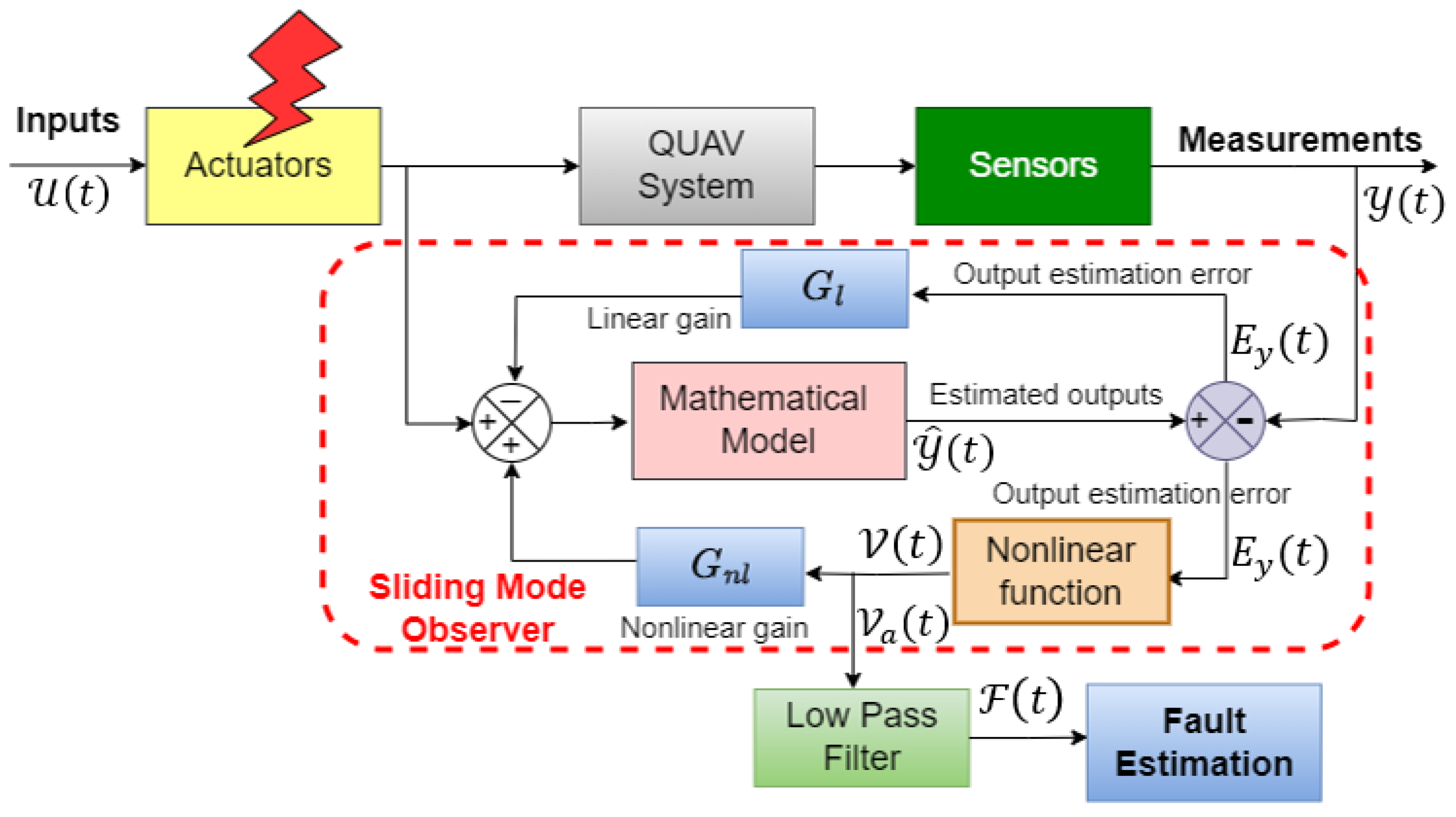
Figure 3 illustrates the architecture employed for actuator fault estimation using the proposed SMO. This architecture is based on the mathematical model for the QUAV, encompassing the dynamics of the system, actuators, and sensors. The model is further expanded to incorporate potential faults in the actuators. Subsequently, an SMO is developed to iteratively reduce the output estimation error to zero, even in the presence of actuator faults. The SMO is driven by the inputs of the QUAV and the output estimation error. This error signal is then fed back into the observer via a nonlinear function to compensate for the effect of actuator faults across the system. In fact, it is found that when the sliding motion occurs, the nonlinear function of the output estimation error, also known as the nonlinear output estimation error, contains information about the actuator faults in the system. As the nonlinear output estimation error is a high-frequency switching signal, we propose the use of a low-pass filter to obtain the signal’s average, thereby estimating the actuator fault.

We implemented the proposed low-pass filter using a first-order differential equation as

$${\dot{\mathcal{V}}}_a\left(t\right)+\delta {\mathcal{V}}_a\left(t\right)={\mathcal{V}}_2\left(t\right),$$

(47)

where ${\mathcal{V}}_a\left(t\right)$ denotes the average of the nonlinear output estimation error ${\mathcal{V}}_2\left(t\right)$, while $\delta$ represents the time constant of the low-pass filter. To ensure accurate fault estimation, it is crucial to select the smallest possible value for the time constant, ensuring it exceeds the sampling time of the computer-implemented low-pass filter.

• Numerical example

We design the SMO for the QUAV system, considering all the state variables as outputs. Therefore, the coordinate transformation used for the SMO design results in

$$T=\left[ \begin{array}{cccccccccccc}1& 0& 0& 0& 0& 0& 0& 0& 0& 0& 0& 0\\ 0& 1& 0& 0& 0& 0& 0& 0& 0& 0& 0& 0\\ 0& 0& 1& 0& 0& 0& 0& 0& 0& 0& 0& 0\\ 0& 0& 0& 1& 0& 0& 0& 0& 0& 0& 0& 0\\ 0& 0& 0& 0& 1& 0& 0& 0& 0& 0& 0& 0\\ 0& 0& 0& 0& 0& 1& 0& 0& 0& 0& 0& 0\\ 0& 0& 0& 0& 0& 0& 1& 0& 0& 0& 0& 0\\ 0& 0& 0& 0& 0& 0& 0& 1& 0& 0& 0& 0\\ 0& 0& 0& 0& 0& 0& 0& 0& 1& 0& 0& 0\\ 0& 0& 0& 0& 0& 0& 0& 0& 0& 1& 0& 0\\ 0& 0& 0& 0& 0& 0& 0& 0& 0& 0& 1& 0\\ 0& 0& 0& 0& 0& 0& 0& 0& 0& 0& 0& 1\end{array} \right].$$

(48)

Since it assumed that all the state variables are measured, both ${\mathcal{A}}_{11}$, and ${\mathcal{A}}_{21}$ are empty matrices, and the matrix ${\mathcal{A}}_{22}$ is equal to the original system matrix $\mathcal{A}$. The design matrix ${\mathcal{A}}_{22}^s$ is defined as

$${\mathcal{A}}_{22}^s=(-10)\ast \left[ \begin{array}{cccccccccccc}1& 0& 0& 0& 0& 0& 0& 0& 0& 0& 0& 0\\ 0& 1& 0& 0& 0& 0& 0& 0& 0& 0& 0& 0\\ 0& 0& 1& 0& 0& 0& 0& 0& 0& 0& 0& 0\\ 0& 0& 0& 1& 0& 0& 0& 0& 0& 0& 0& 0\\ 0& 0& 0& 0& 1& 0& 0& 0& 0& 0& 0& 0\\ 0& 0& 0& 0& 0& 1& 0& 0& 0& 0& 0& 0\\ 0& 0& 0& 0& 0& 0& 1& 0& 0& 0& 0& 0\\ 0& 0& 0& 0& 0& 0& 0& 1& 0& 0& 0& 0\\ 0& 0& 0& 0& 0& 0& 0& 0& 1& 0& 0& 0\\ 0& 0& 0& 0& 0& 0& 0& 0& 0& 1& 0& 0\\ 0& 0& 0& 0& 0& 0& 0& 0& 0& 0& 1& 0\\ 0& 0& 0& 0& 0& 0& 0& 0& 0& 0& 0& 1\end{array} \right].$$

(49)

The linear $G_l$, and nonlinear $G_{nl}$ gain matrices of the SMO are

$$G_l=\left[ \begin{array}{cccccccccccc}10& 1& 0& 0& 0& 0& 0& 0& 0& 0& 0& 0\\ 0& 10& 0& 0& 0& 0& 0& 0& g& 0& 0& 0\\ 0& 0& 10& 1& 0& 0& 0& 0& 0& 0& 0& 0\\ 0& 0& 0& 10& 0& 0& 0& 0& 0& 0& g& 0\\ 0& 0& 0& 0& 10& 1& 0& 0& 0& 0& 0& 0\\ 0& 0& 0& 0& 0& 10& 0& 0& 0& 0& 0& 0\\ 0& 0& 0& 0& 0& 0& 10& 1& 0& 0& 0& 0\\ 0& 0& 0& 0& 0& 0& 0& 10& 0& 0& 0& 0\\ 0& 0& 0& 0& 0& 0& 0& 0& 10& 1& 0& 0\\ 0& 0& 0& 0& 0& 0& 0& 0& 0& 10& 0& 0\\ 0& 0& 0& 0& 0& 0& 0& 0& 0& 0& 10& 1\\ 0& 0& 0& 0& 0& 0& 0& 0& 0& 0& 0& 10\end{array} \right],$$

(50)

and

$$G_{nl}=\left[ \begin{array}{cccccccccccc}1& 0& 0& 0& 0& 0& 0& 0& 0& 0& 0& 0\\ 0& 1& 0& 0& 0& 0& 0& 0& 0& 0& 0& 0\\ 0& 0& 1& 0& 0& 0& 0& 0& 0& 0& 0& 0\\ 0& 0& 0& 1& 0& 0& 0& 0& 0& 0& 0& 0\\ 0& 0& 0& 0& 1& 0& 0& 0& 0& 0& 0& 0\\ 0& 0& 0& 0& 0& 1& 0& 0& 0& 0& 0& 0\\ 0& 0& 0& 0& 0& 0& 1& 0& 0& 0& 0& 0\\ 0& 0& 0& 0& 0& 0& 0& 1& 0& 0& 0& 0\\ 0& 0& 0& 0& 0& 0& 0& 0& 1& 0& 0& 0\\ 0& 0& 0& 0& 0& 0& 0& 0& 0& 1& 0& 0\\ 0& 0& 0& 0& 0& 0& 0& 0& 0& 0& 1& 0\\ 0& 0& 0& 0& 0& 0& 0& 0& 0& 0& 0& 1\end{array} \right],$$

(51)

respectively. The matrix $Q_2$ for the nonlinear discontinuous function $\mathcal{V}\left(t\right)$ results in

$$Q_2=\left(0.05\right)\ast \left[ \begin{array}{cccccccccccc}1& 0& 0& 0& 0& 0& 0& 0& 0& 0& 0& 0\\ 0& 1& 0& 0& 0& 0& 0& 0& 0& 0& 0& 0\\ 0& 0& 1& 0& 0& 0& 0& 0& 0& 0& 0& 0\\ 0& 0& 0& 1& 0& 0& 0& 0& 0& 0& 0& 0\\ 0& 0& 0& 0& 1& 0& 0& 0& 0& 0& 0& 0\\ 0& 0& 0& 0& 0& 1& 0& 0& 0& 0& 0& 0\\ 0& 0& 0& 0& 0& 0& 1& 0& 0& 0& 0& 0\\ 0& 0& 0& 0& 0& 0& 0& 1& 0& 0& 0& 0\\ 0& 0& 0& 0& 0& 0& 0& 0& 1& 0& 0& 0\\ 0& 0& 0& 0& 0& 0& 0& 0& 0& 1& 0& 0\\ 0& 0& 0& 0& 0& 0& 0& 0& 0& 0& 1& 0\\ 0& 0& 0& 0& 0& 0& 0& 0& 0& 0& 0& 1\end{array} \right].$$

(52)

The fault-coupling matrix is represented by $D={\left[0, 0, 0, 0, 0, 0, 0, 0, 0, 0, 0 1\right]}^T$. Since we assume that all the states are measured in this particular case $D=D_2$, and the nonlinear function $\mathcal{V}\left(t\right)={\mathcal{V}}_2\left(t\right)$. The nonlinear function is obtained from Equation (31). The system and input matrices are given by Equation (15), and the output matrix is given by Equation (16).

4.2. Fractional-Order Sliding Mode Observer (FO-SMO)

In recent years, there has been growing interest in adapting classical observers to a fractional-order approach within the realm of control systems. This adaptation offers several advantages over traditional methodologies, providing enhanced capabilities for state estimation in dynamic systems [63]. Historically, classical observers have been preferred due to their simplicity and effectiveness in estimating the state of dynamic systems [64]. In particular, classical sliding mode observers (SMOs), although very effective for the estimation process subject to matched uncertainties, have struggled to adequately capture the fault dynamics due to chattering and their sensitivity to initial conditions and noise [65].

In response to these challenges, we propose a novel approach leveraging fractional-order sliding mode observers (FO-SMOs), which emerges as a promising solution. By integrating fractional-order calculus concepts into the observer design process, this approach offers a more flexible and adaptive framework for fault estimation, capable of accommodating the intricate dynamics of UAV systems while mitigating the effects of disturbances and uncertainties. This proposal aims to explore the potential of FO-SMOs in enhancing fault estimation accuracy and robustness in UAV applications, paving the way for safer and more reliable autonomous operations.

The proposed fractional-order representation of the SMO (referred to in what follows as FO-SMO) is based on the definition presented in Section 2. Applying the Caputo derivative definition of Equation (4) to the SMO given in Equation (43) results in

$${}_0{}^{C}D_t^{{\alpha }_1}\widehat{\mathcal{X}}\left(t\right)=\mathcal{A}\widehat{\mathcal{X}}\left(t\right)+\mathcal{B}\mathcal{U}\left(t\right)-G_l{E}_y\left(t\right)+G_{nl}\mathcal{V}\left(t\right),$$

(53)

and the factional-order representation of the differential equation for the low-pass filter results in

$${}_0{}^{C}D_t^{{\alpha }_2}{\mathcal{V}}_a\left(t\right)=-\delta {\mathcal{V}}_a\left(t\right)+\mathcal{V}\left(t\right).$$

(54)

It is important to note that in Equations (53) and (54), ${\alpha }_1$ and ${\alpha }_2$ represent the orders of the observer and the low-pass filter, respectively. These orders can vary independently, defining this novel approach as a fractional multi-order system. With the system dynamics and low-pass filter now described in different orders, an additional degree of freedom in the system parameters is introduced. One notable advantage of employing the proposed fractional-order sliding mode observer (FO-SMO) is its capability to capture the intricate dynamics inherent in QUAV systems with greater precision. It is important to underline that when both ${\alpha }_1$ and ${\alpha }_2$ are equal to 1, we return to the classical case (integer order). By leveraging fractional-order derivatives and integrals, the FO-SMO presents a more adaptable depiction of system dynamics compared to its integer-order counterpart, the classical SMO. This attribute enhances the observer’s flexibility, empowering it to effectively mitigate the chattering phenomenon and exhibit reduced sensitivity to initial conditions and measurement noise, ensuring more dependable fault estimation.

4.3. Numerical Solution of the FO-SMO

To compute the solutions of both the FO-SMO and the low-pass filter, we use the Grunwald–Letnikov (GL) algorithm presented in Section 2. The solution of the FO-SMO is represented as

$$\widehat{\mathcal{X}}\left(t_k\right)=\left[\mathcal{A}\widehat{\mathcal{X}}\left(t_k\right)+\mathcal{B}\mathcal{U}\left(t_k\right)-G_l{E}_y\left(t_k\right)+G_{nl}\mathcal{V}\left(t_k\right)\right]h^{{\alpha }_1}-\sum _{j=1}^k{c}_j^{{\alpha }_1}\widehat{\mathcal{X}}\left(t_{k-j}\right),$$

(55)

while the solution for the low-pas filter is represented as

$${\mathcal{V}}_a\left(t_k\right)=[-\delta {\mathcal{V}}_a\left(t_k\right)+\mathcal{V}\left(t_k\right)]h^{{\alpha }_2}-\sum _{j=1}^k{c}_j^{{\alpha }_2}{\mathcal{V}}_a\left(t_{k-j}\right)$$

(56)

where $c_j^{{\alpha }_i}=\left(1-\frac{1+{\alpha }_i}{j}\right)c_{j-1}^{{\alpha }_i}$, with $i=$1,2$.$ We performed this numerical solution using MATLAB (latest v. 2024a). For all simulations, we selected the time step $h=0.001$, ${\alpha }_1=0.86$ and ${\alpha }_2=1$.

5. Simulation Results

In this section, we conduct simulations to assess the performance of the proposed observer. We compare the fractional-order sliding mode observer (FO-SMO) with the classical (integer-order) sliding mode observer (SMO) to determine its accuracy and effectiveness in estimating actuator faults in a QUAV system. The parameters of the QUAV utilized in this study are outlined in Table 1. Throughout the simulation, the QUAV is directed to return to its initial position using LQR control, with actuator faults occurring at time $t=0$. These faults are modeled as bounded additive sinusoidal signals adhering to the matching condition. To comprehensively evaluate the observer’s efficacy, we subject it to various operational conditions.

• Experiment Configuration.

To effectively compare the performance of the classical (integer-order) sliding mode observer (SMO) with the proposed fractional-order sliding mode observer (FO-SMO) and to draw meaningful conclusions regarding their suitability for actuator fault estimation, the simulation diagram depicted in Figure 4 was established. This experiment aims to compare the performance of both observers in terms of convergence speed and robustness to initial conditions and measurement noise.

In all our tests, we used the LQR control strategy to stabilize the QUAV at the origin, along with the parameters specified in Table 1. For both observers, the inputs consisted of the actuator signals and measurement outputs. The experiment involved estimating the actuator faults under different operational conditions of the QUAV. First, we considered ideal conditions without measurement noise and evaluated the effect of initial conditions on fault estimation accuracy. Second, we considered the effect of the chattering on fault estimation. Finally, we considered a more realistic scenario where noise was added to all measurement outputs to assess the robustness of both observers to measurement noise. Additionally, we explored the advantages of using a non-integer low-pass filter rather than the classical low-pass filter.

We implemented the observers using the Euler method with a time step of $h=0.001$, and we set the time constant $\delta$ of the low-pass filter to 0.02 for both SMO and FO-SMO. The initial conditions for the observer were established as 0, whereas the initial conditions of the QUAV system varied from zero. The order of the FO-SMO was defined as 0.86.

To quantitatively demonstrate that the performance is better in the FO-SMO than in SMO, we utilize the Normalized Root-Mean-Square Error (NRMSE) criterion. The NRMSE provides a valuable metric for evaluating the accuracy of estimations, expressing the goodness of fit as a percentage, and offering insights into the relative performance of the estimation process. The NRMSE is defined as

$$FIT=\frac{‖{\mathcal{F}}_m\left(:,i\right)-{\mathcal{F}}_e\left(:,i\right)‖}{‖{\mathcal{F}}_m\left(:,i\right)-{mean(\mathcal{F}}_m\left(:,i\right))‖}$$

(57)

In Equation (57), FIT represents the fit of the estimation in terms of the NRMSE, ${\mathcal{F}}_m$ represents the actual fault, ${\mathcal{F}}_e$ represents fault estimation for the observer, and $i$ represents the number of samples.

Case 1.

Robustness to the initial conditions

The initial conditions of the SMO are crucial for ensuring the region and speed of convergence of the observer. These conditions represent the initial state of the observer’s variables, which are used to estimate the system’s state and, in this specific approach, to conduct fault estimation. If the initial conditions of the observer are far from those of the QUAV system, the SMO may fail to converge or converge slowly. Since initial conditions are often unknown in real-world scenarios, ensuring the observer’s robustness to these conditions is essential. Therefore, we conducted simulations to evaluate the robustness of both SMO and FO-SMO to initial conditions. The simulation results compare how well both observers estimate actuator faults under different initial conditions.

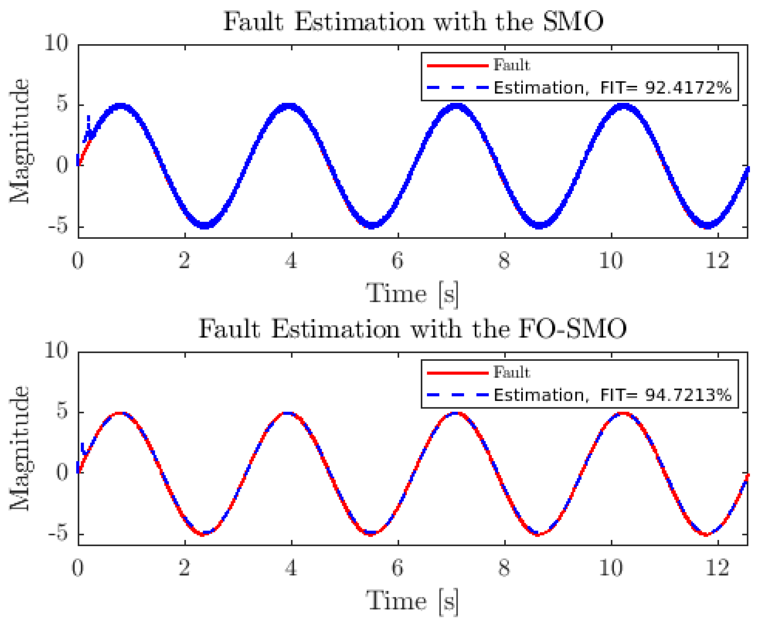
Initially, both observers were initialized to zero, and the initial conditions of the QUAV system were set close, with all states assigned a value of 1. Figure 5 depicts the results of fault estimation using both the FO-SMO and the SMO. The simulation reveals a better performance of the FO-SMO. A sinusoidal signal with an amplitude of 5 was used to simulate the actuator fault. For the FO-SMO and the low-pass filter, fractional orders of ${\alpha }_1=0.86$ and ${\alpha }_2=1$ were employed, respectively. It should be noted that the low-pass filter, in this case, was considered to be of integer order. Notably, the FO-SMO converges more rapidly and exhibits more accurate fault estimation.

In Figure 6, we observe a similar scenario but with a notable difference. The initial conditions of the QUAV were selected further apart compared to the previous case, at a value of 4. In this case, the FIT indicator of the SMO registers at 92.3781%, while the FIT indicator of the FO-SMO stands at 94.2461%. Therefore, we observe that when the initial conditions of the systems and observers are selected far apart, both a reduced convergence rate and a decrease in the FIT of the fault estimation process are presented. Despite these challenging conditions, it is worth noting that the FO-SMO demonstrates superior performance.

In general, we can conclude that when the initial conditions are closer to the true state of the system, the observer is likely to converge faster. Conversely, if the initial conditions are far from the true state, the observer may require more time to adjust its internal variables and converge to an accurate estimate of the system’s state.

Case 2.

Robustness to the chattering

The chattering in SMOs is a well-known issue that can significantly impact their performance. Chattering refers to the rapid switching of nonlinear output injection signals near the sliding surface, resulting in high-frequency oscillations. The presence of chattering in the fault estimation signal can significantly degrade the estimation. Furthermore, since the estimation signal could be utilized to compensate for the fault effect in the control system, this outcome becomes impractical.

The chattering phenomenon in the SMO is heavily influenced by a nonlinear function described in Equation (31), rewritten here for major clarity.

$${\mathcal{V}}_2(t)=\left\{\begin{array}{c}-\rho ‖Q_2‖\frac{Q_2{E}_y\left(t\right)}{‖Q_2{E}_y\left(t\right)‖} \mathrm{if} E_y(t)\ne 0\\ 0 \mathrm{otherwise},\end{array}\right.$$

(58)

In Equation (58), the parameter $\rho$ plays a crucial role in the intensity of chattering. It is important to note that the $\rho$ parameter determines the speed of observer convergence. To ensure an accurate estimation of actuator faults, the value of $\rho$ should be chosen to be greater than the magnitude of the actuator fault. While it is common to use high values for this parameter, doing so can increase chattering. Therefore, it is wise to take a conservative approach. Furthermore, the type of actuator fault being estimated also affects chattering, with fault signals that undergo abrupt changes tending to cause more pronounced chattering.

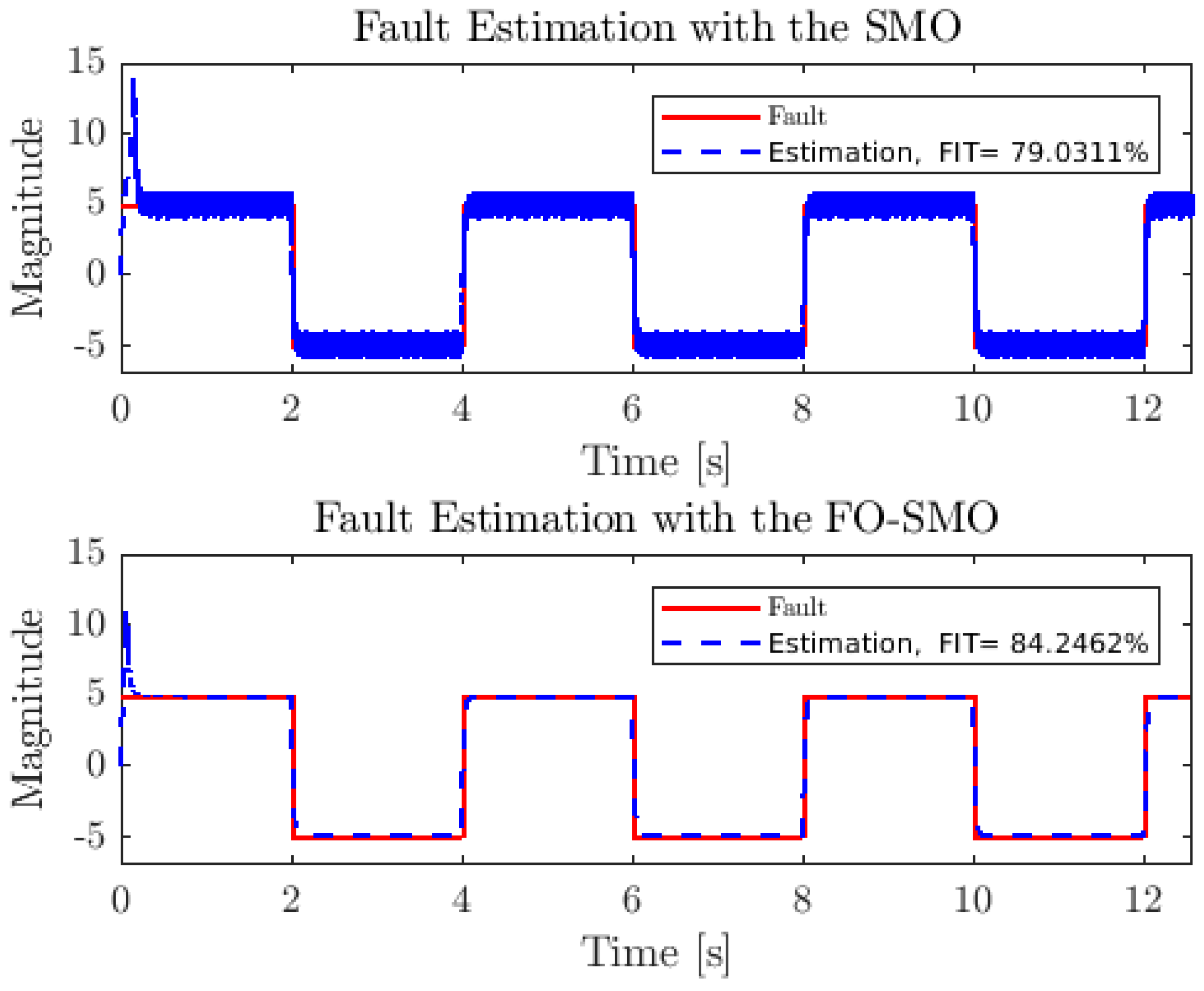
To demonstrate the attenuation properties of the proposed FO-SMO, we compare the performance of both the SMO and the FO-SMO under chattering conditions. To accomplish this, we use a fault signal that exhibits abrupt changes, and we set the $\rho$ value to 20, which is considerably greater than the magnitude of the fault. Under these conditions, the effect of chattering is increased.

In Figure 7, the results of actuator fault estimation under chattering conditions are depicted. There is a significant presence of chattering in the fault estimation of the SMO compared to that observed in Case 1. For the simulation, the initial conditions of the observers were set to 0, while the initial conditions of the QUAV system were set to 2. It is noteworthy that the presence of chattering has degraded the fault estimation in both the SMO and FO-SMO, resulting in FIT values of 79.0311% and 84.2462%, respectively. It is important to emphasize that while selecting $\rho =20$ may have positive effects on increasing the speed of convergence, it also has the adverse effect of increasing chattering, consequently reducing the accuracy of fault estimation. However, the FO-SMO demonstrates superior FIT compared to the classical SMO. Additionally, the high-frequency component is eliminated in the FO-SMO.

Case 3.

Robustness to the measurement noise

In the upcoming tests, we evaluate both the FO-SMO and the SMO under real-world conditions, which involve adding noise to the measured outputs of the QUAV system. This condition allows us to demonstrate that the FO-SMO is more robust to noise than the classical SMO.

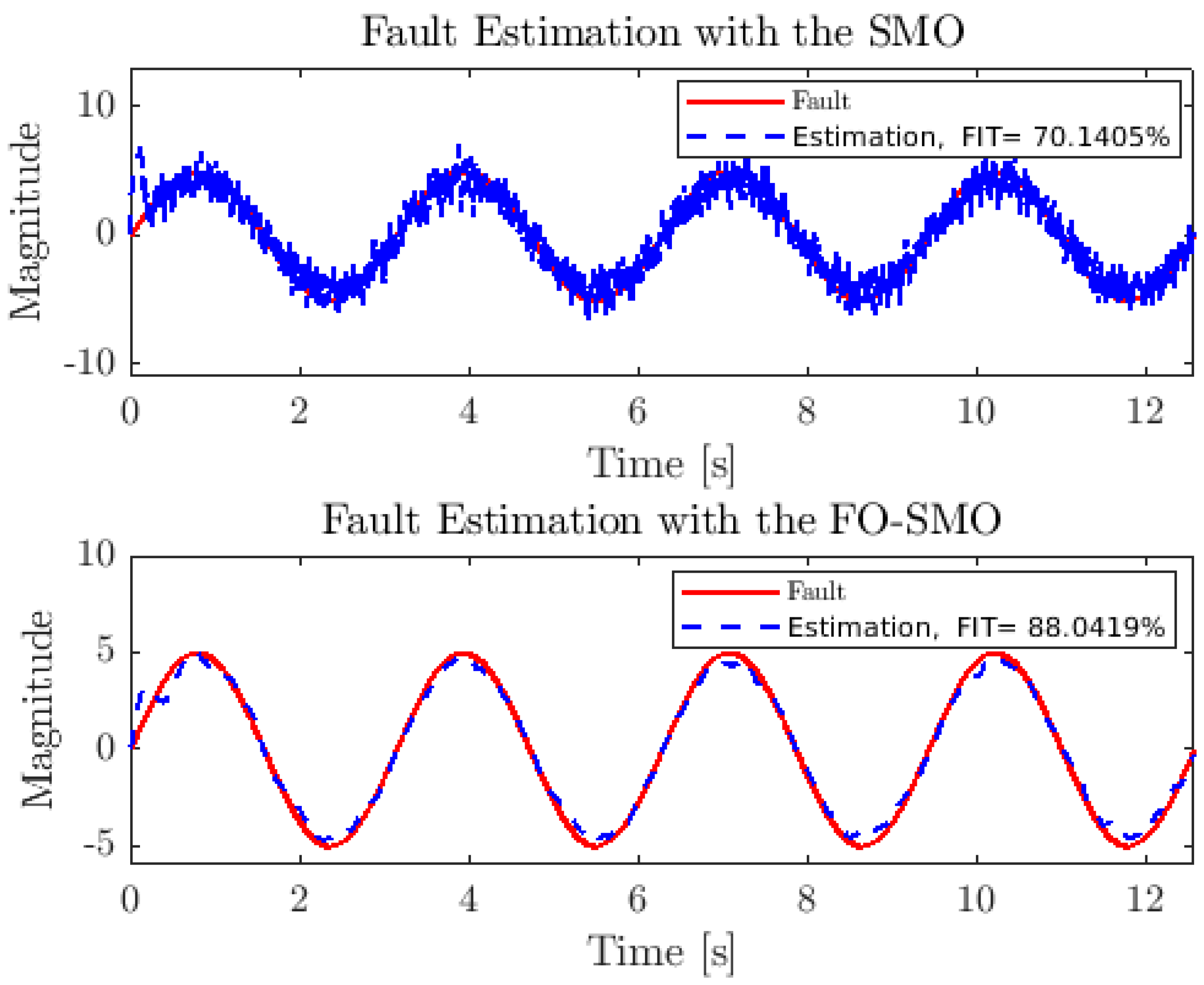
First, noise was introduced to all measurements of the QUAV system. Normally distributed noise is the most common type occurring in natural processes, making the normal distribution an appropriate approximation when exclusively natural noises are incorporated into a signal. To introduce this noise, we utilized the randn function in MATLAB, generating elements that adhere to a normal distribution with a mean of 0 and a variance of 1. The noise was specified as $r\left(t\right)=0.2r and \left(1\right)$. The initial conditions of the observers were set to zero, while those of the QUAV system were chosen at a value of 2. Sinusoidal signals with an amplitude of 5 were used as actuator faults, and the $\rho$ parameter was set to 5. The fractional orders employed for the FO-SMO and the low-pass filter were ${\alpha }_1=0.86$ and ${\alpha }_2=1.7$, respectively. The simulation results of actuator fault estimation using both the SMO and the FO-SMO under noise measurement conditions are presented in Figure 8. It is observed that the addition of noise notably affects the accuracy of the estimated actuator faults, with the FIT for the SMO at 70.1405%, while the FIT for the FO-SMO significantly outperforms it at 88.0419%.

In Figure 9, we observe a scenario similar to the previous one, with a notable difference. A more significant noise measurement has been introduced, specified as $r\left(t\right)=0.6r and \left(1\right)$. The fractional orders employed for the FO-SMO and the low-pass filter were the same as in the above case, and the initial conditions were also set as in the previous case. The simulation results for actuator fault estimation using both the SMO and the FO-SMO under these more severe noise conditions are depicted in Figure 9. Notably, fault estimation using the classical SMO becomes impractical due to the addition of noise. The FIT for the SMO is merely 38.7587%, whereas the FIT for the FO-SMO significantly outperforms it at 82.7243%. This stark contrast highlights the FO-SMO’s remarkable performance in conducting fault estimation under severe noisy conditions. Furthermore, it underscores the effectiveness of employing a fractional-order approach for both the SMO and the low-pass filter, resulting in enhanced fault estimation accuracy even in the presence of measurement noise.

6. Conclusions and Discussion

In this study, we proposed a fractional-order sliding mode observer (FO-SMO) for actuator fault estimation in a QUAV system. Our investigations included comparing the FO-SMO with the classical (integer-order) sliding mode observer (SMO) to assess its correctness and effectiveness. Through rigorous experimentation under various operational conditions of the QUAV, we aimed to ascertain the robustness and accuracy of the FO-SMO in actuator fault estimation. The simulations were meticulously designed, incorporating factors such as initial conditions, chattering, and the influence of measurement noise. We also explored the advantages of employing a non-integer low-pass filter in conjunction with the FO-SMO. Our results indicate that the FO-SMO demonstrates superior performance compared to the classical SMO in fault estimation, particularly under challenging conditions such as noise and chattering. Notably, the FO-SMO exhibited robustness to initial condition variations and effectively mitigated the adverse effects of chattering, resulting in more accurate fault estimation. Furthermore, when subjected to realistic scenarios with added measurement noise, the FO-SMO showcased remarkable resilience and outperformed the classical SMO by a significant margin. The introduction of a fractional-order low-pass filter further enhanced the FO-SMO’s capability to accurately estimate actuator faults, even in the presence of severe noise.

In conclusion, our findings underscore the effectiveness and practicality of the FO-SMO for actuator fault estimation in dynamic systems like QUAVs. By leveraging fractional-order techniques and incorporating robust design considerations, the FO-SMO offers promising prospects for enhancing fault detection and diagnosis in real-world applications. This research contributes valuable insights into the advancement of fault estimation methodologies, paving the way for more reliable and efficient operation of dynamic systems.