Stationary Distribution of Stochastic Age-Dependent Population–Toxicant Model with Markov Switching

Abstract

This work focuses on the convergence of the numerical invariant measure for a stochastic age-dependent population–toxicant model with Markov switching. Considering that Euler–Maruyama (EM) has the advantage of fast computation and low cost, explicit EM was used to discretize the time variable. With the help of the p-th moment boundedness of the analytical and numerical solutions of the model, the existence and uniqueness of the corresponding invariant measures were obtained. Under suitable assumptions, the conclusion that the numerical invariant measure converges to the invariant measure of the analytic solution was proven by defining the Wasserstein distance. A numerical simulation was performed to illustrate the theoretical results.

1. Introduction

The large amount of waste discharged by industrial and agricultural industries has caused serious ecological problems (see [1,2,3]). In particular, the presence of toxicants in the environment is one of the main factors with respect to the reduction in species diversity as well as the extinction of some species. Therefore, it is very important to study the effects of toxicants released in the environment on biological populations by establishing mathematical models. Hallam et al. [4,5] first proposed the deterministic population model in a polluted environment. Next, Liu and Ma [6] established the threshold for the Lotka–Volterra model to analyze the dynamic behavior of a population. Feng and Wang [7] provided some sufficient conditions for weak persistence and extinction. For further details on the results and theory of the deterministic population–toxicant model, see [8,9,10,11].

The aforementioned model parameters are usually assumed to be constants. In fact, in practical problems, the model parameters are affected not only by environmental noise but also by random switching in terms of temperature and climate. In recent years, the stochastic age-dependent population model with Markov switching has attracted the attention of many scholars. For example, Li [12] established a class of stochastic age-dependent population models with Markov switching and proved the convergence of the numerical approximation solution. Then, Ma and Zhang [13] investigated the convergence of the semi-implicit method for the stochastic age-dependent population model. Using Burkholder–Davis–Gundy inequality, Rathinasamy [14] proved that the split-step $\theta$ methods converged to the analytical solutions of the model under given conditions. Motivated by [12,13], Liu et al. [15] proposed a stochastic population model with Markov switching in a polluted environment and obtained the threshold between weak persistence and extinction. However, few authors have studied the stochastic age-dependent population model with Markov switching in a polluted environment. This paper introduces a continuous-time Markov chain into the random parameters of the stochastic age-structured population model in a polluted environment and studies the approximation of its invariant measure.

It is important to find an effective algorithm to approximate the original system’s invariant measure to study the dynamic behavior of a stochastic population. There have been several research results on the invariant measures of stochastic differential equations (see [16,17,18,19]). On the other hand, due to the difficulty of finding general explicit solutions to stochastic differential equations with Markov switching, the numerical approximation method and its ergodic have become interesting hot spots [20,21]. For example, Mao and Yuan [22] investigated the convergence of stationary distributions of EM numerical schemes for stochastic differential equations with Markov switching. Subsequently, under local Lipschitz conditions, Bao [23] proved the approximation of invariant measures for stochastic difference equations with Markov switching. Although the numerical invariant measures for stochastic differential equations have been well studied, there are few studies on the numerical invariant measures of a stochastic age-dependent population model with Markov switching. Based on the ideas of [22,23], in this work, we focus on the existence and uniqueness of the invariant measure for a random age-dependent population–toxicant model with Markov switching using the explicit EM method, which has the advantage of being a simpler calculation, and prove that the numerical invariant measure converges to the underlying invariant measure. Due to the complexity of random population systems with Markov switching, it is difficult to express the exact solution to such a system. Therefore, it is extremely important to develop accurate and efficient numerical approximation methods to calculate the density of populations and toxic substances in population models. However, there are few studies on the numerical approximation of a stochastic age-dependent population model with Markov switching. The main difficulty is that the transition rate matrices of ${\Lambda }_t$ may be different for every step of a jump. The novelties of this study are as follows:

• A stochastic age-dependent population–toxicant model with Markov switching is established. The ergodicity of the invariant measure for this model is obtained, applying stochastic techniques such as Gronwall inequality, Young inequality, and so on.
• Under certain suitable conditions, the explicit EM semi-discrete method is used for the time variables, and the convergence of the numerical invariant measure is analyzed.

The structure of this article is as follows: In Section 2, a new stochastic age-dependent population model is proposed, and some necessary preliminary knowledge is introduced for the following analysis. In Section 3, the existence and uniqueness of the invariant measure for the exact solution under the given conditions are proven, and the boundedness of the p-th moment for the numerical solution is obtained using Gronwall inequality. Furthermore, the convergence of the numerical invariant measure is proven by defining the Wasserstein distance. In Section 4, we verify the theoretical results with numerical examples. The conclusions of this study are presented in Section 5.

2. Model and Preliminaries

2.1. Model Formulation

To begin with, we provide the following stochastic age-dependent population model in a polluted environment, which was proposed by Zhao [24]:

$$\left\{\begin{array}{l}\begin{array}{lll}\frac{\partial P(a,t)}{\partial t} + \frac{\partial P(a,t)}{\partial a}=-\mu (a,t,C_0(t))P(a,t) + g(t,P(a,t))\frac{d{W}_t}{dt},\hfill & & inQ\\ \frac{d{C}_0(t)}{dt}=k(t)C_e(t)-(l(t) + m(t))C_0(t),\hfill & & int\in [0,T]\\ \frac{d{C}_e(t)}{dt}=-h(t)C_e(t) + u(t),\hfill & & int\in [0,T]\\ P(0,t)=\varphi (t)={\int }_0^A\beta (a,t,C_0(t))P(a,t)da,\hfill & & int\in [0,T]\\ P(a,0)=P_0(a),\hfill & & ina\in (0,A)\\ 0 \le C_0(0) \le 1,0 \le C_e(0) \le 1,\hfill \\ N(t)={\int }_0^{A}P(a,t)da.\hfill & & int\in [0,T]\end{array}\hfill \end{array}\right.$$

(1)

All parameters in model (1) are assumed to be positive and are summarized in the Table 1.

Table 1. List of parameters, variables, and their meanings in model (1).

Parameter	Biological Meaning
$P(a,t)$	The density of the population
$m(t)$	The depuration rate of the toxicant
$C_0(t)$	Toxic substances in organisms
$C_e(t)$	Toxic substances in the environment
$l(t)$	The net organismal excretion rate of the toxicant
$\mu (a,t,C_0(t))$	The mortality rate function of the population
$\beta (a,t,C_0(t))$	The fertility rate function of the population
$h(t)$	The total loss rate of the toxicant from the environment
$k(t)$	The net organismal uptake rate of the toxicant from the environment
$g(t,P(a,t))$	The diffusion coefficient dependent on a, t, and $P(a,t)$
$N(t)$	The total density of the population at time t
$u(t)$	The exogenous total toxicant input into the environment at time t

In fact, the parameters of a stochastic age-dependent population model may experience abrupt changes caused by phenomena such as environmental shift in different regimes. Therefore, we can develop a model with regime switching using a finite-state Markov chain. Let ${\Lambda }_t,$$t>0$ be a right-continuous Markov chain in the probability space taking values in a finite state of $S=\{1,2,\dots ,N\}$ for some positive integer ($N<\infty$) with transition rules being specified by

$$\mathbb{P}({\Lambda }_{t+\Delta }=j|{\Lambda }_t=i)=\left\{\begin{array}{cc}{q}_{ij}\Delta + o(\Delta ),\hfill & i\ne j,\\ 1 + q_{ii}\Delta + o(\Delta ),\hfill & i=j,\end{array}\right.$$

(2)

where $\Delta >0$, $o(\Delta )$ denotes that ${lim}_{\Delta \to 0}\frac{o(\Delta )}{\Delta }=0$. $q_{ij}$ is the transition rate from state i to j satisfying $q_{ii}=-{\displaystyle \sum _{i\ne j}}{q}_{ij}$. We assume that the Markov chain ($\{{\Lambda }_t\}$) is independent of ${\{W_t\}}_{t\ge 0}$ and that the transition matrix ($Q:={(q_{ij})}_{N\times N}$) is irreducible and conservative. Under this condition, the Markov chain has a unique stationary distribution ($\pi =({\pi }_1,{\pi }_2,\dots ,{\pi }_N)\in R^{1\times N}$), which can be determined by solving the equation $\pi Q=\mathbf{0}$ (where $\mathbf{0}$ is zero vector) subject to ${\displaystyle \sum _{k=1}^N}{\pi }_k=1$ and ${\pi }_k>0$, $\forall k\in S$.

Inspired by [15], we introduce colored noise (i.e., the Markov chain) into the stochastic age-dependent population model (1). The following model is obtained:

$$\left\{\begin{array}{l}\begin{array}{lll}\frac{\partial P(a,t)}{\partial t} + \frac{\partial P(a,t)}{\partial a}=-\mu (a,t,C_0(t),{\Lambda }_t)P(a,t) + g(t,P(a,t),{\Lambda }_t)\frac{d{W}_t}{dt},\hfill & & inQ\\ \frac{d{C}_0(t)}{dt}=k({\Lambda }_t)C_e(t)-(l({\Lambda }_t) + m({\Lambda }_t))C_0(t),\hfill & & int\in [0,T]\\ \frac{d{C}_e(t)}{dt}=-h({\Lambda }_t)C_e(t) + u(t),\hfill & & int\in [0,T]\\ P(0,t)=\varphi (t)={\int }_0^A\beta (a,t,C_0(t),{\Lambda }_t)P(a,t)da,\hfill & & int\in [0,T]\\ P(a,0)=x_1=P_0(a),\hfill & & ina\in (0,A)\\ 0 \le C_0(0) \le 1,0 \le C_e(0) \le 1,\hfill \\ N(t)={\int }_0^{A}P(a,t)da,\hfill & & int\in [0,T]\end{array}\hfill \end{array}\right.$$

(3)

where $Q=(0,A)\times [0,T],$$P_0(a)$ is the initial population density.

Remark 1. 

The parameters of the system are not constant but randomly switch over time. The system can use many biological models: susceptible–infected–recovered (SIR), susceptible–infected–vaccinated (SIV), the Lotka–Volterra model, and so on. Our future work will focus on sensitivity analysis of the system.

Remark 2. 

In the real world, population systems are usually affected by random perturbations in the environment, such as seasons, temperature, and so on. In addition, the jump due to instantaneous changes (e.g., high temperature, a rainstorm, and policy implementation) in the state of the population system need to be taken into account [25]. To depict these phenomena, it is necessary to introduce non-Gaussian noise, such as the Lévy process, a discontinuous function with right continuity and left limits [26]. The stochastic population models driven by Lévy noise are rarely analyzed for the control problem. This will also be part of our future work.

2.2. Preliminaries

• Let $(\Omega ,\mathcal{F},\mathbb{P})$ be a complete probability space with ${\{{\mathcal{F}}_t\}}_{0\le t\le T}$ as the natural filtration generated by Brownian motion ($W_t$), which means ${\mathcal{F}}_t=\sigma \{W_s;0 \le s \le t\}$ augmented with all P-null sets of ${\mathcal{F}}_0$.
• $\mathbb{E}$ stands for the expectation corresponding to $\mathbb{P}$.
• C denotes a positive constant whose value may change in different occurrences.
• $V=H^1([0,A])\equiv \{\phi |\phi \in L^2([0,A]),\frac{\partial \phi }{\partial a}\in L^2([0,A])$, where $\frac{\partial \phi }{\partial a}$ represents generalized partial derivatives, and is a Sobolev space.
• $⟨·,·⟩$ denotes the duality product between V and $V^{\prime }$, and $(·,·)$ is the scalar product in H.

For an operator ($B\in \mathcal{L}(M,H)$) in the space of all bounded linear operators from M into H, we $|·|$ denotes the norm in H ($H=L^2([0,A])$) such that

$$V\hookrightarrow H\equiv H^{\prime }\hookrightarrow V^{\prime }.$$

(4)

The integral version of Equation (3) is given by the following equation:

$$\left\{\begin{array}{c}\begin{array}{c}{P}_t=x_1-{\int }_0^t[\frac{\partial P(s)}{\partial a} + \mu (a,s,C_0(s),{\Lambda }_s)P(s)]ds + {\int }_0^{t}g(s,P(s),{\Lambda }_s)d{W}_s,\hfill \\ C_0=x_2 + {\int }_0^t[k({\Lambda }_t)C_e(t)-(l({\Lambda }_t) + m({\Lambda }_t))C_0(t)]ds,\hfill \\ C_e=x_3 + {\int }_0^t[-h({\Lambda }_t)C_e(t) + u(t)]ds,\hfill \end{array}\hfill \end{array}\right.$$

(5)

where $P(a,0)=x_1,C_0(0)=x_2,C_e(0)=x_3$, $g(t,·,i):S\times L_H^2\to \mathcal{L}(M,H)$ is the family of nonlinear operators, and ${\mathcal{F}}_t$ is almost surely measurable in t.

Now, let us provide the following necessary assumptions:

Assumption 1. 

Assume

$$\begin{array}{c}0 \le \beta (a,t,C_0(t),{\Lambda }_t) \le \overline{\beta }<\infty ,0 \le {\mu }_0 \le \mu (a,t,C_0(t),{\Lambda }_t) \le \overline{\mu }<\infty ,\hfill \\ k_0 + h_0 \le k({\Lambda }_t) + h({\Lambda }_t) \le \widehat{k} + \widehat{h}<\infty ,l_0 + m_0 \le l({\Lambda }_t) + m({\Lambda }_t) \le \widehat{M}<\infty ,\hfill \end{array}$$

(6)

where $\overline{\beta }$, $\widehat{k}$, $\widehat{h}$, $\widehat{M}$, and $\overline{\mu }$ denote positive constants.

Assumption 2. 

There exists a positive constant ${\psi }_i$ such that for $i\in \mathbb{S}$, $t\in [0,T]$,

$$\parallel g(t,P^{x_1,i}(t),i)-g(t,P^{{\overline{x}}_1,i}(t),i){\parallel }^2 \le {\psi }_i{|P^{x_1,i}(t)-P^{{\overline{x}}_1,i}(t)|}^2,$$

(7)

where $x_1$ and ${\overline{x}}_1$ are the two different initial values.

Further, for each $i\in \mathbb{S}$ and $P^{x_1,i}(t)\in H$, $t\in [0,T]$,

$$\parallel g(t,P^{x_1,i}(t),i){\parallel }^2 \le L + {\psi }_i{|P^{x_1,i}(t)|}^2,$$

(8)

where L depends on the initial value of the function $g(t,0,i)$.

Assumption 3. 

Assume

$$0 \le u_0 \le u(t) \le \overline{u}<\infty ,$$

(9)

where $\overline{u}$ is a positive constant.

Remark 3. 

Assumption 1 implies that the coefficients of system (5) are all finite numbers and non-negative. Assumption 2 guarantees the existence and uniqueness of the solution for system (5). From a biological point of view, Assumption 3 indicates that the exogenous total toxicant input is finite.

We replace $((P(t),C_0(t),C_e(t)),{\Lambda }_t)$ with $((P^{x_1,i}(t),C_0^{x_2,i}(t),C_e^{x_3,i}(t)),{\Lambda }_t^i)$, especially the initial value $((P(0),C_0(0),C_e(0)),{\Lambda }_0)=((x_1,x_2,x_3),i)\in H\times \mathbb{R}\times \mathbb{R}\times \mathbb{S}.$ For any $p\in (0,1]$, setting $x:=(x_1,x_2,x_3)$, the norm of vector $x-\overline{x}$ in space $\mathbb{H}:=H\times R\times R$ is defined as $|x-\overline{x}|:=\sqrt{|x_1-{\overline{x}}_1| + |x_2-{\overline{x}}_2| + |x_3-{\overline{x}}_3|}$. We define a metric on $\mathbb{H}\times \mathbb{S}$ as follows:

$$\begin{array}{c}{d}_p((x,i),(\overline{x},i)):={\int }_{\mathbb{H}}{|x-\overline{x}|}^p + I_{\{i\ne j\}},(x,i),(\overline{x},i)\in \mathbb{H}\times \mathbb{S},\hfill \end{array}$$

where $I_G$ denotes the indicator function of set G, and $\overline{x}=({\overline{x}}_1,{\overline{x}}_2,{\overline{x}}_3)$ is a different initial value. For $p\in (0,1]$, we define the Wasserstein distance between $\nu \in \mathcal{P}(\mathbb{H}\times \mathbb{S})$ and ${\nu }^{\prime }\in \mathcal{P}(\mathbb{H}\times \mathbb{S})$ by

$$W_p(\nu ,{\nu }^{\prime })=inf\mathbb{E}{d}_p(X_k,X_{k^{\prime }}),$$

where the infimum is taken over all pairs of random variables ($X_k$, $X_{k^{\prime }}$ on $\mathbb{H}\times \mathbb{S}$ with respective laws $\nu$, ${\nu }^{\prime }$). Let ${\mathbb{P}}_t((x_1,x_2,x_3),i;·)$ be the transition probability kernel of the pair $((P^{x_1,i}(t),C_0^{x_2,i}(t),C_e^{x_3,i}(t)),{\Lambda }_t^i)$, a time-homogeneous Markov process (see [27]). Recall that $\pi \in \mathcal{P}(\mathbb{H}\times \mathbb{S})$ is called an invariant measure of $((P^{x_1,i}(t),C_0^{x_2,i}(t),C_e^{x_3,i}(t)),{\Lambda }_t^i)$ if

$$\pi (A\times \{i\})=\sum _{j=1}^N{\int }_{\mathbb{H}}{\mathbb{P}}_t((x_1,x_2,x_3),j;A\times \{i\})\pi (d(x_1,x_2,x_3)\times \{j\}),t\ge 0,A\in \mathbb{H},i\in \mathbb{S}$$

(10)

holds. For any $p>0$, let

$$diag(\rho )\triangleq diag({\rho }_1,\dots ,{\rho }_N),Q_p\triangleq Q + \frac{p}{2}diag(\rho ),{\eta }_p\triangleq -\underset{\gamma }{max}Re\gamma ,$$

(11)

where ${\rho }_i$ is a positive constant, and $\gamma \in \mathrm{spec}(Q_p)$, $\mathrm{spec}(Q_p)$ denotes the spectrum of $Q_p$ (i.e., the multi-set of its eigenvalues). $Re\gamma$ is the real part of $\gamma$, and $diag({\rho }_1,\dots ,{\rho }_N)$ denotes the diagonal matrix whose diagonal entries starting in the upper-left corner are ${\rho }_1,\dots ,{\rho }_N$, respectively.

3. Invariant Measure

With the help of the p-th moment boundedness of the analytical and numerical solutions of the model, the existence and uniqueness of the corresponding invariant measures are obtained. Under suitable assumptions, the conclusion that the numerical invariant measure converges to the invariant measure of the analytic solution is proven by defining the Wasserstein distance.

Under Assumptions 1–3, using the method similar to that described in [28], we can prove the existence and uniqueness of the solution. Therefore, it is omitted. In this section, we first prove the existence and uniqueness of the corresponding invariant measure. Then, we discuss the numerical invariant measure of the Euler–Maruyama method and the convergence of the numerical invariant measure under the Wasserstein measure.

3.1. Invariant Measure of Exact Solution

Theorem 1. 

Let $N<\infty$ and Assumptions 1–3 hold with ${max}_{i\in S}{\rho }_i>0$. Then, the exact solution of system (3) admits a unique invariant measure ($\pi \in \mathcal{P}(\mathbb{H}\times \mathbb{S})$).

Proof. 

Let $((P^{x_1,i}(t),C_0^{x_2,i}(t),C_e^{x_3,i}(t)),{\Lambda }_t^i)$ be the exact solution of Equation (3) with $((x_1,x_2,x_3),i)$ as initial values, where $((x_1,x_2,x_3),i)\in \mathbb{H}\times \mathbb{S}$. A simple application of the Feynman–Kac formula shows that $Q_{p,t}=e^{t{Q}_p}$, where $Q_p$ is given in Equation (11). Then, the spectral radius (Ria$(Q_{p,t})$, i.e., Ria$(Q_{p,t})={sup}_{\lambda \in \mathrm{spec}(Q_{p,t})}|\lambda |$) of $Q_{p,t}$ equals $e^{-{\eta }_{p}t}.$ Since all coefficients of $Q_{p,t}$ are positive, the Perron–Frobenius theorem (see, e.g., [29]) shows that $-{\eta }_p$ is a simple eigenvalue of $Q_p$, all other eigenvalues having a strictly smaller real part. Note that the eigenvector of $Q_{p,t}$ corresponding to $e^{-{\eta }_{p}t}$ is also an eigenvector of $Q_p$ corresponding to $-{\eta }_p$. According to the Perron–Frobenius theorem, for $Q_p$, it can be found that there is a positive eigenvector (${\xi }^{(p)}=({\xi }_1^{(p)},\dots ,{\xi }_N^{(p)})\gg \mathbf{0}$, where $\mathbf{0}\in \mathbb{H}$ is a zero vector) corresponding to the eigenvalue $-{\eta }_p$, and ${\xi }^{(p)}\gg \mathbf{0}$ means that each component is ${\xi }_i^{(p)}>0$. Let

$$p_0=1\wedge \underset{i\in \mathbb{S},{\rho }_i>0}{min}\{-2q_{ii}/{\rho }_i\}.$$

(12)

Combined with Lemma 2.1 of [23], we can obtain

$$Q_p{\xi }_i^{(p)}=-{\eta }_p{\xi }_i^{(p)}\ll \mathbf{0},$$

(13)

and

$$\underset{t\ge 0}{sup}\mathbb{E}(|P^{x_1,i}{(t)|}^p + |C_0^{x_2,i}{(t)|}^p + |C_e^{x_3,i}(t){|}^p) \le C.$$

(14)

Furthermore,

$$\begin{array}{cc}& e^{{\eta }_{p}t}\mathbb{E}((1 + |C_e^{x_3,i}{(t)|}^2{)}^{p/2}{\xi }_{{\Lambda }_t^i}^{(p)})\hfill \\ \hfill =& (1 + |x_3{|}^2{)}^{\frac{p}{2}}{\xi }_i^{(p)} + \mathbb{E}{\int }_0^t{e}^{{\eta }_{p}s}(1 + |C_e^{x_3,i}(s){{|}^2)}^{\frac{p}{2}}\left\{{\eta }_p{\xi }_{{\Lambda }_s^i}^{(p)} + (Q{\xi }^{(p)})({\Lambda }_s^i)\right\}ds\hfill \\ & + \mathbb{E}{\int }_0^t{e}^{{\eta }_{p}s}\left\{\frac{p}{2}(1 + |C_e^{x_3,i}(s){{|}^2)}^{\frac{p-2}{2}}2⟨C_e^{x_3,i}(s),-h({\Lambda }_s^i)C_e^{x_3,i}(s) + u(s)⟩\right\}{\xi }_{{\Lambda }_s^i}^{(p)}ds\hfill \\ \hfill \le & (1 + |x_3{|}^2{)}^{\frac{p}{2}}{\xi }_i^{(p)} + \frac{p}{2}\mathbb{E}{\int }_0^t{e}^{{\eta }_{p}s}(1 + |C_e^{x_3,i}{(s)|}^2{)}^{\frac{p-2}{2}}K(1 + |C_e^{x_3,i}(s){|}^2){\xi }_{{\Lambda }_s^i}^{(p)}ds,\hfill \end{array}$$

(15)

where $K:=max\{\overline{u},2(\widehat{h} + \widehat{k}) + 1\}$ is a positive constant. In the last step, we use the fundamental inequality ($2ab \le a^2 + b^2$) for any $a,b \le 0$. Finally, using Gronwall inequality and taking the sup on both sides of Equation (15), we obtain the following result:

$$\underset{t\ge 0}{sup}\mathbb{E}|C_e^{x_3,i}{(t)|}^p \le C(1 + |x_3{|}^p).$$

(16)

Using similar methods, it is not difficult to obtain

$$\underset{t\ge 0}{sup}\mathbb{E}|C_0^{x_2,i}{(t)|}^p \le C(1 + |x_2{|}^p).$$

(17)

On the other hand, according to the Itô formula, for any $p\in (0,p_0)$, we can obtain

$$\begin{array}{cc}& e^{{\eta }_{p}t}\mathbb{E}((1 + |P^{x_1,i}{(t)|}^2{)}^{p/2}{\xi }_{{\Lambda }_t^i}^{(p)})\hfill \\ =\hfill & (1 + |x_1{|}^2{)}^{\frac{p}{2}}{\xi }_i^{(p)} + \mathbb{E}{\int }_0^t{e}^{{\eta }_{p}s}(1 + |P^{x_1,i}(s){{|}^2)}^{\frac{p}{2}}\left\{{\eta }_p{\xi }_{{\Lambda }_s^i}^{(p)} + (Q{\xi }^{(p)})({\Lambda }_s^i)\right\}ds\hfill \\ & + \mathbb{E}{\int }_0^t{e}^{{\eta }_{p}s}\{\frac{p}{2}(1 + |P^{x_1,i}{(s)|}^2{)}^{-1}(2⟨P_s^{x_1,i},-\frac{\partial P^{x_1,i}(s)}{\partial a}\hfill \\ & -\mu (a,t,C_0(t),{\Lambda }_s^i)P^{x_1,i}(s)⟩ + \parallel g(s,P^{x_1,i}(s),{\Lambda }_s^i){\parallel }^2){\xi }_{{\Lambda }_s^i}^{(p)}\hfill \\ & + \frac{p(p-2)}{2}(1 + |P^{x_1,i}{(s)|}^2{)}^{-2}\parallel P^{x_1,i}(s)*g(s,P^{x_1,i}(s),{\Lambda }_s^i){\parallel }^2{\xi }_{{\Lambda }_s^i}^{(p)}\}(1 + |P^{x_1,i}(s){{|}^2)}^{\frac{p}{2}}ds,\hfill \end{array}$$

(18)

due to $\frac{p(p-2)}{2}<0$ and

$$\begin{array}{cc}⟨P^{x_1,i}(s),-\frac{\partial P^{x_1,i}(s)}{\partial a}⟩\hfill & =-{\int }_0^A{P}^{x_1,i}(s)d_a(P^{x_1,i}(s))=\frac{1}{2}{({\int }_0^A\beta (a,t,C_0(t),{\Lambda }_t)P^{x_1,i}(s)da)}^2\hfill \\ & \le \frac{1}{2}{\int }_0^A{\beta }^2(a,t,C_0(t),{\Lambda }_t)da{\int }_0^A{(P^{x_1,i}(s))}^{2}da\hfill \\ & \le \frac{1}{2}{A}^2{\overline{\beta }}^2{|P^{x_1,i}(s)|}^2.\hfill \end{array}$$

(19)

It follows from Equation (18) that

$$\begin{array}{cc}& e^{{\eta }_{p}t}\mathbb{E}((1 + |P^{x_1,i}{(t)|}^2{)}^{p/2}{\xi }_{{\Lambda }_t^i}^{(p)})\hfill \\ \le \hfill & (1 + |x_1{|}^2{)}^{\frac{p}{2}}{\xi }_i^{(p)} + \mathbb{E}{\int }_0^t{e}^{{\eta }_{p}s}\{\frac{p}{2}(1 + |P^{x_1,i}{(s)|}^2{)}^{-1}((2\overline{\mu } + A^2{\overline{\beta }}^2){|P^{x_1,i}(s)|}^2\hfill \\ & + \parallel g(s,P^{x_1,i}(s),{\Lambda }_s^i){\parallel }^2) + {\eta }_p{\xi }_{{\Lambda }_s^i}^{(p)} + Q{\xi }^{(p)}({\Lambda }_s^i)\}{\xi }_{{\Lambda }_s^i}^{(p)}(1 + |P^{x_1,i}(s){{|}^2)}^{\frac{p}{2}}ds\hfill \\ \le \hfill & (1 + |x_1{{|}^2)}^{\frac{p}{2}}{\xi }_i^{(p)} + \mathbb{E}{\int }_0^t{e}^{{\eta }_{p}s}\left\{\frac{p}{2}(1 + |P^{x_1,i}{(s)|}^2{)}^{\frac{p}{2}-1}(L + \overline{C}|P^{x_1,i}(s){|}^2)\right\}{\xi }_{{\Lambda }_s^i}^{(p)}ds\hfill \\ \le \hfill & C(1 + |x_1{|}^p) + \frac{p}{2}\mathbb{E}{\int }_0^t{e}^{{\eta }_{p}s}R(1 + |P^{x_1,i}(s){{|}^2)}^{\frac{p}{2}}{\xi }_{{\Lambda }_s^i}^{(p)}ds,\hfill \end{array}$$

(20)

where $\overline{C}=2\overline{\mu } + A^2{\overline{\beta }}^2 + {\psi }_i$, $R:=max\{\overline{C},L\}$. Then, according to the Gronwall inequality and taking sup over $t\ge 0$ for Equation (21), we have

$$\underset{t\ge 0}{sup}\mathbb{E}|P^{x_1,i}{(t)|}^p \le C(1 + |x_1{|}^p).$$

(21)

Equations (16), (17), and (21) lead to Equation (14).

In order to show the uniqueness and ergodicity of invariant measures, based on references [19,22,30], we can define a probability measure

$${\chi }_t(A):=\frac{1}{t}{\int }_0^t{\mathbb{P}}_s(x,i;A)ds,\forall t>0,A\in (\mathbb{H}\times \mathbb{S}).$$

Then, for any $\epsilon >0$, according to Equation (21) and Chebyshev’s inequality, there exists a sufficiently large $r>0$ such that

$$\begin{array}{cc}{\chi }_t(K_r\times \mathbb{S})\hfill & =\frac{1}{t}{\int }_0^t{\mathbb{P}}_s(x,i;K_r\times \mathbb{S})ds\hfill \\ & \ge 1-\frac{{sup}_{t\ge 0}E(|P_t^{x_1,i}{|}^p + |C_0^{x_2,i}{(t)|}^p + |C_e^{x_3,i}(t){|}^p)}{r^p}\ge 1-\epsilon .\hfill \end{array}$$

(22)

Hence, ${\chi }_t$ is tight, due to the compact embedding ($V⋐\mathbb{H}$); then, $K_r=\{x\in \mathbb{H};|x| \le r\}$ is a compact subset of $\mathbb{H}$. Borrowing the proof method of [[23], Theorem 2.3], ${\sigma }^{*}>0$ is constant such that $W_p({\Delta }_{((x_1,x_2,x_2),i)}{\mathbb{P}}_t,{\Delta }_{(({\overline{x}}_1,{\overline{x}}_2,{\overline{x}}_3),j)}{\mathbb{P}}_t) \le C{e}^{-{\sigma }^{*}t}$ holds. Therefore, conclusions about the existence and uniqueness of the result for the invariant measure can be obtained but omit details to avoid repetition. □

3.2. Numerical Invariant Measure

The simulation of a discrete Markov chain was proposed in [27]. Now, let $t_1,t_2,\dots ,t_m$ be deterministic grid points of $[0,T]$. $\Delta =t_{k+1}-t_k$ denotes increments of time. $t_k=k\Delta$, $k\ge 1$, $\Delta =\frac{T}{N} \le 1$. For system (5), we can define the discrete-time Euler–Maruyama approximate solution ($P_{\Delta }^{x_1,i}(t_{k+1})\approx P^{x_1,i}(t_{k+1})$, $C_{0,\Delta }^{x_2,i}(t_{k+1})\approx C_0^{x_2,i}(t_{k+1})$, $C_{e,\Delta }^{x_3,i}(t_{k+1})\approx C_e^{x_3,i}(t_{k+1})$ on $t=0,\Delta ,2\Delta ,\dots ,N\Delta$) using the following iterative scheme:

$$\left\{\begin{array}{c}\begin{array}{c}{P}_{\Delta }^{x_1,i}(t_{k+1})=P_{\Delta }^{x_1,i}(t_k)-[\frac{\partial P_{\Delta }^{x_1,i}(t_{k+1})}{\partial a} + \mu (a,t_k,C_0(t_k),{\Lambda }_{t_k}^i)P_{\Delta }^{x_1,i}(t_k)]\Delta \hfill \\ + g(t_k,P_{\Delta }^{x_1,i}(t_k),{\Lambda }_{t_k}^i)\Delta W_k,\hfill \\ C_{0,\Delta }^{x_2,i}(t_{k+1})=C_{0,\Delta }^{x_2,i}(t_k) + [k({\Lambda }_{t_k}^i)C_{e,\Delta }^{x_3,i}(t_k)-(l({\Lambda }_{t_k}^i) + m({\Lambda }_{t_k}^i))C_{0,\Delta }^{x_2,i}(t_k)]\Delta ,\hfill \\ C_{e,\Delta }^{x_3,i}(t_{k+1})=C_{e,\Delta }^{x_3,i}(t_k) + [-h({\Lambda }_{t_k}^i)C_{e,\Delta }^{x_3,i}(t_k) + u(t_k)]\Delta .\hfill \end{array}\hfill \end{array}\right.$$

(23)

where the initial values are $P_{\Delta }(0)=x_1$, $C_{0,\Delta }(0)=x_2$, $C_{e,\Delta }(0)=x_3$, ${\Lambda }_0=i$, $P_{\Delta }^{x_1,i}(t_k,0)={\int }_0^A\beta (a,t_k,C_0(t_k),{\Lambda }_{t_k}^i)P_{\Delta }^{x_1,i}(t_k)da$, and $\Delta W_k=W_{k+1}-W_k$ is Brownian motion. Then

$$\left\{\begin{array}{c}\begin{array}{c}{P}_{\Delta }^{x_1,i}(t)=x_1-{\int }_0^t[\frac{\partial P_{\Delta }^{x_1,i}(s)}{\partial a} + \mu (a,\lfloor s/\Delta \rfloor \Delta ,C_0(s),{\Lambda }_{\lfloor s/\Delta \rfloor \Delta }^i){\overline{P}}_{\Delta }^{x_1,i}(\lfloor s/\Delta \rfloor \Delta )]ds\hfill \\ + {\int }_0^{t}g(\lfloor s/\Delta \rfloor \Delta ,{\overline{P}}_{\Delta }^{x_1,i}(\lfloor s/\Delta \rfloor \Delta ),{\Lambda }_{\lfloor t/\Delta \rfloor \Delta }^i)d{W}_s,\hfill \\ C_{0,\Delta }^{x_2,i}(t)=x_2 + {\int }_0^t[k({\Lambda }_{\lfloor s/\Delta \rfloor \Delta }^i){\overline{C}}_{e,\Delta }^{x_3,i}(\lfloor s/\Delta \rfloor \Delta )-(l({\Lambda }_{\lfloor s/\Delta \rfloor \Delta }^i) + m({\Lambda }_{\lfloor s/\Delta \rfloor \Delta }^i)){\overline{C}}_{0,\Delta }^{x_2,i}(\lfloor s/\Delta \rfloor \Delta )]ds,\hfill \\ C_{e,\Delta }^{x_3,i}(t)=x_3 + {\int }_0^t[-h({\Lambda }_{\lfloor s/\Delta \rfloor \Delta }^i){\overline{C}}_{e,\Delta }^{x_3,i}(\lfloor s/\Delta \rfloor \Delta ) + u(\lfloor s/\Delta \rfloor \Delta )]ds,\hfill \end{array}\hfill \end{array}\right.$$

(24)

where for ${\Lambda }_0^i=i\in \mathbb{S}$, ${\overline{P}}_{\Delta }^{x_1,i}(t)={\sum }_{k=0}^N{P}_{\Delta }^{x_1,i}(t_k)I_{[t_k,t_{k+1})}(t)$, ${\overline{C}}_{0,\Delta }^{x_2,i}(t)={\sum }_{k=0}^N{C}_{0,\Delta }^{x_2,i}(t_k)I_{[t_k,t_{k+1})}(t)$, ${\overline{C}}_{e,\Delta }^{x_3,i}(t)={\sum }_{k=0}^N{C}_{e,\Delta }^{x_3,i}(t_k)I_{[t_k,t_{k+1})}(t)$. $I_G$ is the indicator function of set G. By a straightforward calculation, one has $P_{\lfloor t/\Delta \rfloor \Delta }^{x_1,i}={\overline{P}}_{\lfloor t/\Delta \rfloor \Delta }^{x_1,i}$, $C_{0,\lfloor t/\Delta \rfloor \Delta }^{x_2,i}={\overline{C}}_{0,\lfloor t/\Delta \rfloor \Delta }^{x_2,i}$, $C_{e,\lfloor t/\Delta \rfloor \Delta }^{x_3,i}={\overline{C}}_{e,\lfloor t/\Delta \rfloor \Delta }^{x_3,i}$, $t\ge 0$ (i.e., the discrete-time EM scheme (23) coincides with the corresponding continuous-time EM scheme (24) at the grid points whenever they enjoy the same starting points). $\lfloor a\rfloor$ denotes the integer part of a.

By a similar method [19], we set $X_k^{x,i}:=(P_k^{x_1,i},C_{0,k}^{x_2,i},C_{e,k}^{x_3,i})$ and $x:=(x_1,x_2,x_3)$, $Z_k^{x,i}=(X_k^{x,i},{\Lambda }_k^i)$. ${\{Z_k^{x,i}\}}_{k\ge 0}$ is a non-homogenous Markov process with transition probability kernel ${\mathbb{P}}_{m\Delta ,k\Delta }^{\Delta }(x,j;A\times \{i\}):=\mathbb{P}(X_{k\Delta }^{x,i}\in A\times \{i\}|X_{m\Delta }^{x,j}=(x,j))$, $\forall k\ge m\ge 0.$ If ${\pi }^{\Delta }\in \mathcal{P}(H\times \mathbb{S})$ satisfies

$${\pi }^{\Delta }(A\times \{i\})=\sum _{j=1}^N{\int }_{\mathbb{H}}{\mathbb{P}}_{k\Delta }^{\Delta }(x,j;A\times \{i\}){\pi }^{\Delta }(dx\times \{j\}),k\ge 0,A\in \mathbb{H},i\in \mathbb{S},$$

(25)

then ${\pi }^{\Delta }$ is called an invariant measure of $(X_k^{x_x,i},{\Lambda }_k^i)$. Let

$$q_0:=\underset{i\in \mathbb{S}}{max}(-q_{ii}),{\rho }_0=\underset{i\in \mathbb{S}}{max}|{\rho }_i|,\widehat{{\xi }_0}\triangleq \underset{i\in \mathbb{S}}{max}{\xi }_i^{(p)},\breve{{\xi }_0}\triangleq {(\underset{i\in \mathbb{S}}{max}{\xi }_i^{(p)})}^{-1},$$

$$J^{*}:=max\{3p{4}^p({\psi }_0 + \overline{\mu })(q_0\widehat{{\xi }_0}\breve{{\xi }_0} + {\overline{\mu }}^{\frac{p}{2}}),4^{1+p}p{\psi }_0[3^{\frac{p}{2}}({\overline{\mu }}^2 + {\psi }_0) + q_0\widehat{{\xi }_0}\breve{{\xi }_0}]\}.$$

To prove the p-th moment boundedness of the numerical solution for the EM scheme, first, we cite the classical conclusion in the next Lemma (see [31]).

Lemma 1 

(In Mao [31]). Let $h(x,w)$ be a scalar bounded measurable random function of x independent of ${\mathcal{F}}_s$, and let ζ be an ${\mathcal{F}}_s$-measurable random variable. Then,

$$\mathbb{E}(h(\zeta ,w)|{\mathcal{F}}_s)=H(\zeta ),$$

(26)

where $H(\zeta )=\mathbb{E}h(x,w)$.

Lemma 1 provides great convenience for proof of Lemma 2. The following lemma shows that the continuous approximation is bounded.

Lemma 2. 

Under Assumptions 1–3, if

$$\Delta <\frac{1}{4{({\psi }_0 + \overline{u})}^2}\wedge \frac{1}{2g^{*}}\wedge \frac{1}{8{\overline{\mu }}^2}\wedge {(\frac{{\eta }_p-e^{*}}{J^{*}})}^{2/p},$$

(27)

then we have

$$\begin{array}{c}\underset{t\in [0,T]}{sup}\mathbb{E}(|P_{\Delta }^{x_1,i}{(t)|}^p + |C_{0,\Delta }^{x_2,i}{(t)|}^p + |C_{e,\Delta }^{x_3,i}{(t)|}^p) \le C(|x_1{|}^p + |x_2{|}^p + |x_3{|}^p),\hfill \end{array}$$

(28)

where $g^{*}:=max\{\widehat{k} + \widehat{h},\widehat{M}\}$ and $e^{*}:=p(\overline{\mu } + A^2{\overline{\beta }}^2)$ for any $p\in (0,p_0),$ and the initial values are$((x_1,x_2,x_3),i)\in \mathbb{H}\times \mathbb{S}$.

Proof. 

In the following proof, let $W_{t,\Delta }={|W_t-W_{\lfloor t/\Delta \rfloor \Delta }|}^2$ and

$${\overline{P}}_{\Delta }^{x_1,i}:={\overline{P}}_{\Delta }^{x_1,i}(\lfloor t/\Delta \rfloor \Delta ),{\overline{C}}_{0,\Delta }^{x_2,i}:={\overline{C}}_{e,\Delta }^{x_2,i}(\lfloor t/\Delta \rfloor \Delta ),{\overline{C}}_{e,\Delta }^{x_3,i}:={\overline{C}}_{e,\Delta }^{x_3,i}(\lfloor t/\Delta \rfloor \Delta ).$$

First, by (8), one obtains from (24) that

$$\begin{array}{cc}|{\overline{P}}_{\Delta }^{x_1,i}|\hfill & \le |P_{\Delta }^{x_1,i}(t)| + (|\frac{\partial P_{\Delta }^{x_1,i}(t)}{\partial a}| + |\overline{\mu }{\overline{P}}_{\Delta }^{x_1,i}|)\Delta + |g(\lfloor t/\Delta \rfloor \Delta ,{\overline{P}}_{\Delta }^{x_1,i},{\Lambda }_{\lfloor t/\Delta \rfloor \Delta }^i)|\sqrt{W_{t,\Delta }}\hfill \\ & \le |P_{\Delta }^{x_1,i}(t)| + |\frac{\partial P_{\Delta }^{x_1,i}(t)}{\partial a}|\Delta + \overline{\mu }|{\overline{P}}_{\Delta }^{x_1,i}|\Delta + (L + {\psi }_0|{\overline{P}}_{\Delta }^{x_1,i}|)\sqrt{W_{t,\Delta }},\hfill \end{array}$$

(29)

and

$$\begin{array}{c}|P_{\Delta }^{x_1,i}(t)-{\overline{P}}_{\Delta }^{x_1,i}| \le (|\frac{\partial P_{\Delta }^{x_1,i}(t)}{\partial a}| + |\overline{\mu }{\overline{P}}_{\Delta }^{x_1,i}|)\Delta + (L + {\psi }_0|{\overline{P}}_{\Delta }^{x_1,i}|)\sqrt{W_{t,\Delta }}.\hfill \end{array}$$

(30)

Therefore, taking $\Delta <\frac{1}{8{\overline{\mu }}^2}$, we arrive at

$$\begin{array}{cc}|{\overline{P}}_{\Delta }^{x_1,i}{|}^2\hfill & \le 4|P_{\Delta }^{x_1,i}{(t)|}^2 + 4|\frac{\partial P_{\Delta }^{x_1,i}(t)}{\partial a}{|}^2{\Delta }^2 + 4{\overline{\mu }}^2|{\overline{P}}_{\Delta }^{x_1,i}{|}^2{\Delta }^2 + 4(L + {\psi }_0|{\overline{P}}_{\Delta }^{x_1,i}{|)}^2{W}_{t,\Delta }\hfill \\ & \le 4|P_{\Delta ,t}^{x_1,i}{|}^2 + 4|\frac{\partial P_{\Delta }^{x_1,i}(t)}{\partial a}{|}^2\Delta + 4{\overline{\mu }}^2|{\overline{P}}_{\Delta }^{x_1,i}{|}^2\Delta + 4(L + {\psi }_0|{\overline{P}}_{\Delta }^{x_1,i}{|)}^2{W}_{t,\Delta }\hfill \\ & \le 8|P_{\Delta }^{x_1,i}{(t)|}^2 + 8|\frac{\partial P_{\Delta }^{x_1,i}(t)}{\partial a}{|}^2\Delta + 8(L + {\psi }_0|{\overline{P}}_{\Delta }^{x_1,i}{|)}^2{W}_{t,\Delta },\hfill \end{array}$$

(31)

and

$$\begin{array}{cc}|P_{\Delta }^{x_1,i}(t)-{\overline{P}}_{\Delta }^{x_1,i}{|}^2\hfill & \le 4|\frac{\partial P_{\Delta }^{x_1,i}(t)}{\partial a}{|}^2{\Delta }^2 + 4|\overline{\mu }{\overline{P}}_{\Delta }^{x_1,i}{|}^2{\Delta }^2 + 2(L + {\psi }_0|{\overline{P}}_{\Delta }^{x_1,i}{|)}^2{W}_{t,\Delta }\hfill \\ & \le 32{\overline{\mu }}^2|P_{\Delta }^{x_1,i}{(t)|}^2{\Delta }^2 + 36{\overline{\mu }}^2|\frac{\partial P_{\Delta }^{x_1,i}(t)}{\partial a}{|}^2{\Delta }^2 + 6(L + {\psi }_0|{\overline{P}}_{\Delta }^{x_1,i}{|)}^2{W}_{t,\Delta }.\hfill \end{array}$$

(32)

Next, by applying the Itô formula for $p\in (0,p_0)$ and $\rho >0$, we can obtain

$$\begin{array}{cc}& e^{\rho t}\mathbb{E}((1 + |P_{\Delta }^{x_1,i}{(t)|}^2{)}^{p/2}{\xi }_{{\Lambda }_t^i}^{(p)})\hfill \\ \le \hfill & (1 + |x_1{|}^2{)}^{p/2}{\xi }_i^{(p)} + \mathbb{E}{\int }_0^t{e}^{\rho s}\left\{\rho {\xi }_{{\Lambda }_s^i}^{(p)} + (Q{\xi }^{(p)})({\Lambda }_s^i)\right\}(1 + |P_{\Delta }^{x_1,i}(s){{|}^2)}^{p/2}ds\hfill \\ & + \mathbb{E}{\int }_0^t{e}^{\rho s}(1 + |P_{\Delta }^{x_1,i}{(s)|}^2{)}^{\frac{p}{2}}{\xi }_{{\Lambda }_s^i}^{(p)}\{\frac{p}{2}(1 + |P_{\Delta }^{x_1,i}(s){{|}^2)}^{-1}(2⟨P_{\Delta }^{x_1,i}(s),-\frac{\partial P_{\Delta }^{x_1,i}(s)}{\partial a}⟩\hfill \\ & -2⟨P_{\Delta }^{x_1,i}(s),\overline{\mu }{\overline{P}}_{\Delta }^{x_1,i}⟩ + {\parallel g(\lfloor s/\Delta \rfloor \Delta ,{\overline{P}}_{\Delta }^{x_1,i},{\Lambda }_{\lfloor s/\Delta \rfloor \Delta }^i)\parallel }^2){\xi }_{{\Lambda }_s^i}^{(p)}\hfill \\ & + \frac{p(p-2)}{2}(1 + |P_{\Delta }^{x_1,i}{(s)|}^2{)}^{-2}\parallel P_{\Delta }^{x_1,i}(s)*g(\lfloor s/\Delta \rfloor \Delta ,{\overline{P}}_{\Delta }^{x_1,i},{\Lambda }_{\lfloor s/\Delta \rfloor \Delta }^i),{\Lambda }_s^i{)\parallel }^2\}ds,\hfill \end{array}$$

(33)

Using inequality Equation (19) and $p(p-2)<0$, we can obtain

$$\begin{array}{cc}& e^{\rho t}\mathbb{E}((1 + |P_{\Delta }^{x_1,i}{(t)|}^2{)}^{p/2}{\xi }_{{\Lambda }_t^i}^{(p)})\hfill \\ \le \hfill & (1 + |x_1{|}^2{)}^{p/2}{\xi }_i^{(p)} + \mathbb{E}{\int }_0^t{e}^{\rho s}\left\{\rho {\xi }_{{\Lambda }_s^i}^{(p)} + (Q{\xi }^{(p)})({\Lambda }_s^i)\right\}(1 + |P_{\Delta }^{x_1,i}(s){{|}^2)}^{p/2}ds\hfill \\ & + \mathbb{E}{\int }_0^t{e}^{\rho s}\{\frac{p}{2}(1 + |P_{\Delta }^{x_1,i}{(s)|}^2{)}^{-1}(2⟨P_{\Delta ,s}^{x_0,i},\overline{\mu }{\overline{P}}_{\Delta }^{x_1,i}⟩ + A^2{\overline{\beta }}^2{|P_{\Delta }^{x_1,i}(s)|}^2\hfill \\ & + \parallel g(\lfloor s/\Delta \rfloor \Delta ,{\overline{P}}_{\Delta }^{x_1,i},{\Lambda }_{\lfloor s/\Delta \rfloor \Delta }^i){\parallel }^2){\xi }_{{\Lambda }_s^i}^{(p)}\}(1 + |P_{\Delta }^{x_1,i}(s){{|}^2)}^{p/2}ds\hfill \\ \le \hfill & (1 + |x_1{|}^2{)}^{p/2}{\xi }_i^{(p)} + C{e}^{\rho t} + \mathbb{E}{\int }_0^t{e}^{\rho s}\left\{\rho {\xi }_{{\Lambda }_s^i}^{(p)} + (Q{\xi }^{(p)})({\Lambda }_s^i)\right\}(1 + |P_{\Delta }^{x_1,i}(s){{|}^2)}^{p/2}ds\hfill \\ & + \mathbb{E}{\int }_0^t{e}^{\rho s}\left\{\frac{p}{2}(1 + |P_{\Delta }^{x_1,i}(s){{|}^2)}^{\frac{p-2}{2}}\left(I_1 + (9\overline{\mu } + A^2{\overline{\beta }}^2){|P_{\Delta }^{x_1,i}(s)|}^2\right){\xi }_{{\Lambda }_s^i}^{(p)}\right\}ds,\hfill \end{array}$$

(34)

where $I_1:=({\psi }_0 + \overline{\mu }){|{\overline{P}}_{\Delta }^{x_1,i}|}^2$, ${\psi }_0:=\underset{i\in \mathbb{S}}{max}|{\psi }_i|$. By using the conclusion of [32], for any $s \le \Delta$, due to $q_{ii}<0$, we have

$$\begin{array}{c}\mathbb{P}({\Lambda }_s^i\ne {\Lambda }_0^i)=1-\mathbb{P}({\Lambda }_s^i={\Lambda }_0^i) \le 1-e^{q_{ii}s} \le 1-e^{q_{ii}\Delta } \le -q_{ii}\Delta \le q_0\Delta .\hfill \end{array}$$

(35)

Applying the results of Lemma 1, we obtain

$$\begin{array}{c}\mathbb{E}(|P_{\Delta }^{x_1,i}{(\lfloor s/\Delta \rfloor \Delta )|}^p){\mathbf{1}}_{{\Lambda }_{\lfloor s/\Delta \rfloor \Delta }^i\ne {\Lambda }_s^i})\hfill \\ =\mathbb{E}(\mathbb{E}((|P_{\Delta }^{x_1,i}{(\lfloor s/\Delta \rfloor \Delta )|}^p){\mathbf{1}}_{{\Lambda }_{\lfloor s/\Delta \rfloor \Delta }^i\ne {\Lambda }_s^i})|{\mathcal{F}}_{\lfloor s/\Delta \rfloor \Delta })\hfill \\ =\mathbb{E}((|P_{\Delta }^{x_1,i}{(\lfloor s/\Delta \rfloor \Delta )|}^p)\mathbb{E}({\mathbf{1}}_{{\Lambda }_{\lfloor s/\Delta \rfloor \Delta }^i\ne {\Lambda }_s^i}|{\Lambda }_{\lfloor s/\Delta \rfloor \Delta }^i))\hfill \\ \le q_0\Delta \mathbb{E}(|P_{\Delta }^{x_1,i}(\lfloor s/\Delta \rfloor \Delta ){|}^p),\hfill \end{array}$$

(36)

where ${\{W_t\}}_{t\ge 0}$ is independent of ${\{{\Lambda }_t\}}_{t\ge 0}$. Furthermore, due to $\frac{\partial \phi }{\partial a}\in L^2([0,A])$, we have ${\int }_0^T{|\frac{\partial \phi }{\partial a}|}^{2}ds<C<\infty$. In addition, in the light of Equations (36) and (32), taking $\Delta <\frac{1}{4\overline{\mu }}$, it follows that

$$\begin{array}{cc}& \frac{p}{2}\mathbb{E}{\int }_0^t{e}^{\rho s}(1 + |P_{\Delta }^{x_1,i}(s){{|}^2)}^{\frac{p-2}{2}}{I}_1{\xi }_{{\Lambda }_s^i}^{(p)}ds\hfill \\ & =\frac{p}{2}\mathbb{E}{\int }_0^t{e}^{\rho s}(1 + |P_{\Delta }^{x_1,i}{(s)|}^2{)}^{\frac{p-2}{2}}({\psi }_0 + \overline{\mu }){|{\overline{P}}_{\Delta }^{x_1,i}|}^2{\xi }_{{\Lambda }_s^i}^{(p)}ds\hfill \\ \le \hfill & p({\psi }_0 + \overline{\mu })\mathbb{E}{\int }_0^t{e}^{\rho s}(1 + |P_{\Delta }^{x_1,i}(s){|}^2{)}^{\frac{p-2}{2}}{|P_{\Delta }^{x_1,i}(s)-{\overline{P}}_{\Delta }^{x_1,i}|}^2{\mathbf{1}}_{\{{\Lambda }_{\lfloor s/\Delta \rfloor \Delta }^i\ne {\Lambda }_s^i\}}{\xi }_{{\Lambda }_s^i}^{(p)}ds\hfill \\ & + p({\psi }_0 + \overline{\mu })\mathbb{E}{\int }_0^t{e}^{\rho s}(1 + |P_{\Delta }^{x_1,i}(s){|}^2{)}^{\frac{p-2}{2}}{|P_{\Delta }^{x_1,i}(s)|}^2{\mathbf{1}}_{\{{\Lambda }_{\lfloor s/\Delta \rfloor \Delta }^i\ne {\Lambda }_s^i\}}{\xi }_{{\Lambda }_s^i}^{(p)}ds\hfill \\ \le \hfill & 3p({\psi }_0 + \overline{\mu })\mathbb{E}{\int }_0^t{e}^{\rho s}(1 + |P_{\Delta }^{x_1,i}(s){{|}^2)}^{\frac{p}{2}}{\mathbf{1}}_{\{{\Lambda }_{\lfloor s/\Delta \rfloor \Delta }^i\ne {\Lambda }_s^i\}}{\xi }_{{\Lambda }_s^i}^{(p)}ds\hfill \\ & + 3p({\psi }_0 + \overline{\mu })\mathbb{E}{\int }_0^t{e}^{\rho s}(1 + |P_{\Delta }^{x_1,i}(s){|}^2{)}^{\frac{p-2}{2}}{|\frac{\partial P_{\Delta }^{x_1,i}(s)}{\partial a}|}^2{\mathbf{1}}_{\{{\Lambda }_{\lfloor s/\Delta \rfloor \Delta }^i\ne {\Lambda }_s^i\}}{\xi }_{{\Lambda }_s^i}^{(p)}ds\hfill \\ \le \hfill & C{e}^{\rho t} + 3p{2}^{\frac{p}{2}}({\psi }_0 + \overline{\mu })\widehat{{\xi }_0}\mathbb{E}{\int }_0^t{e}^{\rho s}{|{\overline{P}}_{\Delta }^{x_1,i}|}^p{\mathbf{1}}_{\{{\Lambda }_{\lfloor s/\Delta \rfloor \Delta }^i\ne {\Lambda }_s^i\}}ds\hfill \\ & + 3p{2}^{\frac{p}{2}}({\psi }_0 + \overline{\mu })\mathbb{E}{\int }_0^t{e}^{\rho s}{|P_{\Delta }^{x_1,i}(s)-{\overline{P}}_{\Delta }^{x_1,i}|}^p{\mathbf{1}}_{\{{\Lambda }_{\lfloor s/\Delta \rfloor \Delta }^i\ne {\Lambda }_s^i\}}{\xi }_{{\Lambda }_s^i}^{(p)}ds\hfill \\ \le \hfill & C{e}^{\rho t} + 3p{4}^p({\psi }_0 + \overline{\mu })(q_0\widehat{{\xi }_0}\breve{{\xi }_0} + {\overline{\mu }}^{\frac{p}{2}}){\Delta }^{\frac{p}{2}}{\int }_0^t{e}^{\rho s}\mathbb{E}((1 + |P_{\Delta }^{x_1,i}(s){|}^2{)}^{\frac{p}{2}}{\xi }_{{\Lambda }_s^i}^{(p)})ds,\hfill \end{array}$$

(37)

where in the above inequality, we mainly use the fundamental inequality (${(c + d)}^{\theta } \le c^{\theta } + d^{\theta }$) for any $c,d>0$ and $\theta \in (0,1)$. Therefore, according to Equations (34) and (37), we have

$$\begin{array}{cc}& e^{\rho t}\mathbb{E}((1 + |P_{\Delta }^{x_1,i}{(t)|}^2{)}^{p/2}{\xi }_{{\Lambda }_t^i}^{(p)})\hfill \\ \le \hfill & C(1 + |x_1{|}^p + e^{\rho t}) + \mathbb{E}{\int }_0^t{e}^{\rho s}(\rho -{\eta }_p)(1 + |P_{\Delta }^{x_1,i}(s){{|}^2)}^{p/2}{\xi }_{{\Lambda }_s^i}^{(p)}ds\hfill \\ & + \mathbb{E}{\int }_0^t{e}^{\rho s}\left\{\frac{p}{2}(1 + |P_{\Delta }^{x_1,i}(s){{|}^2)}^{-1}\left(I_1 + (9\overline{\mu } + A^2{\overline{\beta }}^2){|P_{\Delta }^{x_1,i}(s)|}^2\right){\xi }_{{\Lambda }_s^i}^{(p)}\right\}(1 + |P_{\Delta }^{x_1,i}(s){{|}^2)}^{p/2}ds\hfill \\ \le \hfill & C(1 + |x_1{|}^p + e^{\rho t})-({\eta }_p-\alpha {\Delta }^{\frac{p}{2}}-\rho -\frac{p}{2}(9\overline{\mu } + A^2{\overline{\beta }}^2))\mathbb{E}{\int }_0^t{e}^{\rho s}(1 + |P_{\Delta }^{x_1,i}(s){{|}^2)}^{p/2}{\xi }_{{\Lambda }_s^i}^{(p)}ds,\hfill \end{array}$$

(38)

where $\alpha :=3p{4}^p({\psi }_0 + \overline{\mu })(q_0\widehat{{\xi }_0}\breve{{\xi }_0} + {\overline{\mu }}^{\frac{p}{2}})$, taking $\rho ={\eta }_p-J^{*}{\Delta }^{\frac{p}{4}}-p(9\overline{\mu } + A^2{\overline{\beta }}^2)>0$. According to Gronwall inequality and taking the upper bound on the left-hand side of Equation (38), we obtain

$$\begin{array}{c}\underset{t\in [0,T]}{sup}\mathbb{E}(1 + |P_{\Delta }^{x_1,i}{(s)|}^p) \le C(1 + |x_1{|}^p)e^{-(J^{*}{\Delta }^{\frac{p}{4}}-\alpha {\Delta }^{\frac{p}{2}}-\frac{p}{2}(9\overline{\mu } + A^2{\overline{\beta }}^2))T} \le C(1 + |x_1{|}^p).\hfill \end{array}$$

(39)

On the other hand, by repeating the same procedure, taking $\Delta <\frac{1}{2(\widehat{k} + \widehat{h})}$, we have

$$|{\overline{C}}_{e,\Delta }^{x_3,i}| \le 2|C_{e,\Delta }^{x_3,i}(t)| + 2\overline{u}\Delta ,$$

(40)

and

$$\begin{array}{cc}|{\overline{C}}_{0,\Delta }^{x_2,i}|\hfill & \le |C_{0,\Delta }^{x_2,i}(t)| + \widehat{M}|{\overline{C}}_{0,\Delta }^{x_2,i}|\Delta + (\widehat{k} + \widehat{h})|{\overline{C}}_{e,\Delta }^{x_3,i}|\Delta \hfill \\ & \le 2|C_{0,\Delta }^{x_2,i}(t)| + 2|C_{e,\Delta }^{x_3,i}(t)| + 2\overline{u}\Delta .\hfill \end{array}$$

(41)

Therefore, combining Equation (24) and Equation (40), the following result can be obtained:

$$\begin{array}{cc}|C_{e,\Delta }^{x_3,i}{(t)|}^2\hfill & \le 2|x_3{|}^2 + 2{\int }_0^t[{(g^{*})}^2|{\overline{C}}_{e,\Delta }^{x_3,i}(s){|}^2 + 2{\overline{u}}^2]ds\hfill \\ & \le 2|x_3{|}^2 + 32{(g^{*})}^2{\int }_0^t(|C_e^{x_3,i}(s){|}^2 + {\overline{u}}^2{\Delta }^2)ds + 4{\int }_0^t{\overline{u}}^{2}ds,\hfill \end{array}$$

(42)

Applying H$\ddot{o}$lder inequality and taking the sup of Equation (42), it follows that

$$\begin{array}{c}\underset{s\in [0,t]}{sup}|C_{e,\Delta }^{x_3,i}{(t)|}^p \le C(1 + |x_3{|}^2{)}^{\frac{p}{2}} + 4^{\frac{5p}{4}}{c}_t{(g^{*})}^p\mathbb{E}{\int }_0^t(\underset{s\in [0,t]}{sup}|C_e^{x_3,i}(s){|}^p)ds,\hfill \end{array}$$

(43)

where $c_t$ is a positive constant related to time t. Then, according to Gronwall inequality, Equation (43) becomes

$$\underset{t\in [0,T]}{sup}{|C_{e,\Delta }^{x_3,i}(t)|}^p \le C.$$

(44)

Using a similar method, applying the results of Equations (39) and (40), it then follows that

$$\begin{array}{cc}|C_{0,\Delta }^{x_2,i}{(t)|}^2\hfill & \le 3|x_2{|}^2 + 3{(g^{*})}^2{\int }_0^t|{\overline{C}}_{e,\Delta }^{x_3,i}(s){|}^{2}ds + 3{\widehat{M}}^2{\int }_0^t{|{\overline{C}}_{0,\Delta }^{x_2,i}(s)|}^{2}ds\hfill \\ & \le 3|x_2{|}^2 + h^{*}{\int }_0^t(|C_{e,\Delta }^{x_3,i}{(s)|}^2 + {\overline{u}}^2{\Delta }^2)ds + 36{\widehat{M}}^2{\int }_0^t{|C_{0,\Delta }^{x_2,i}(s)|}^{2}ds,\hfill \end{array}$$

(45)

due to Equation (27), H$\ddot{o}$lder inequality, and the following equation:

$$(h^{*}{\int }_0^t(|C_{e,\Delta }^{x_3,i}{(s)|}^2 + {\overline{u}}^2{\Delta }^2{)ds)}^{\frac{p}{2}} \le {(h^{*})}^{\frac{p}{2}}{c}_t{\int }_0^t{|C_{e,\Delta }^{x_3,i}(s)|}^{p}ds + {(h^{*}(\overline{u}T))}^{\frac{p}{2}},$$

where $h^{*}:=24{(g^{*})}^2 + 36{\widehat{M}}^2$ is a positive constant, and according to Gronwall inequality, one can obtain

$$\underset{t\in [0,T]}{sup}{|C_{0,\Delta }^{x_2,i}(t)|}^p \le C.$$

(46)

Finally, the results of Equations (39), (44), and (46) show that Lemma 2 holds.

□

To investigate the uniqueness of the numerical invariant measure, we provide the asymptotically attractive property of the numerical solutions of the implicit EM scheme.

Lemma 3. 

Under the conditions of Theorem 1, we assume that $\mathbb{E}[|\frac{\partial \phi }{\partial a}{|}^2]<C$ and $\overline{\mu }>\frac{3g^{*}}{4}$ and that there exists a sufficiently small ${\Delta }^{*}$ such that for any $\Delta \in (0,{\Delta }^{*})$, the numerical solutions of the implicit EM scheme satisfy

$$\begin{array}{c}\mathbb{E}(|P_{\Delta }^{x_1,i}(t)-P_{\Delta }^{{\overline{x}}_1,j}(t){|}^p + |C_{0,\Delta }^{x_2,i}(t)-C_{0,\Delta }^{{\overline{x}}_2,j}(t){|}^p + |C_{e,\Delta }^{x_3,i}(t)-C_{e,\Delta }^{{\overline{x}}_3,j}(t){|}^p)\hfill \\ \le C(1 + |x_1{|}^p + |{\overline{x}}_1{|}^p + |x_2{|}^p + |{\overline{x}}_2{|}^p + |x_3{|}^p + |{\overline{x}}_3{|}^p)e^{-\tilde{\sigma }t},\hfill \end{array}$$

(47)

for any $p\in (0,p_0)$, $p_0$ is given in (12), $((x_1,x_2,x_2),i),(({\overline{x}}_1,{\overline{x}}_2,{\overline{x}}_3),j)\in \mathbb{H}\times \mathbb{S}$, $g^{*}$ is introduced in Lemma 2, and $\tilde{\sigma }$ is a positive constant.

Proof. 

Equation (29) and Lemma 2 imply that

$$\begin{array}{cc}|{\overline{P}}_{\Delta }^{x_1,i}-{\overline{P}}_{\Delta }^{{\overline{x}}_1,i}| \le \hfill & |P_{\Delta }^{x_1,i}(t)-P_{\Delta }^{{\overline{x}}_1,i}(t)| + |\frac{\partial (P_{\Delta }^{x_1,i}(t)-P_{\Delta }^{{\overline{x}}_1,i}(t))}{\partial a}|\Delta \hfill \\ & + \overline{\mu }|{\overline{P}}_{\Delta }^{x_1,i}-{\overline{P}}_{\Delta }^{{\overline{x}}_1,i}|\Delta + ({\psi }_0|{\overline{P}}_{\Delta }^{x_1,i}-{\overline{P}}_{\Delta }^{{\overline{x}}_1,i}|)\sqrt{W_{t,\Delta }}\hfill \\ \hfill \le & 2|P_{\Delta }^{x_1,i}(t)-P_{\Delta }^{{\overline{x}}_1,i}(t)| + 2|\frac{\partial (P_{\Delta }^{x_1,i}(t)-P_{\Delta }^{{\overline{x}}_1,i}(t))}{\partial a}|\Delta ,\hfill \end{array}$$

(48)

such that

$$|{\overline{P}}_{\Delta }^{x_1,i}-{\overline{P}}_{\Delta }^{{\overline{x}}_1,i}{|}^2 \le 8{|P_{\Delta }^{x_1,i}(t)-P_{\Delta }^{{\overline{x}}_1,i}(t)|}^2 + 8{\psi }^{*}{\Delta }^2,$$

(49)

and

$$|P_{\Delta }^{x_1,i}(s)-P_{\Delta }^{{\overline{x}}_1,i}(s)-({\overline{P}}_{\Delta }^{x_1,i}-{\overline{P}}_{\Delta }^{{\overline{x}}_1,i}){|}^2 \le 24u^{*}{|P_{\Delta }^{x_1,i}(t)-P_{\Delta }^{{\overline{x}}_1,i}(t)|}^2 + 11{\psi }^{*}{\Delta }^2,$$

(50)

where $u^{*}:={\overline{\mu }}^2{\Delta }^2 + {\psi }_0{\Delta }^{\frac{1}{2}}$ and ${\psi }^{*}:={|\frac{\partial (P_{\Delta }^{x_1,i}(t)-P_{\Delta }^{{\overline{x}}_1,i}(t))}{\partial a}|}^2$. For any $\epsilon >0$ and $\rho >0$, according to the Itô formula and Equation (19), it follows from Assumptions 1–3 that

$$\begin{array}{cc}& \mathbb{E}(e^{\rho t}(\epsilon + |P_{\Delta }^{x_1,i}(t)-P_{\Delta }^{{\overline{x}}_1,i}{(t)|}^2{)}^{\frac{p}{2}}{\xi }_{{\Lambda }_t^i}^{(p)})\hfill \\ \le \hfill & (\epsilon + |x_1-{\overline{x}}_1{|}^2{)}^{p/2}{\xi }_i^{(p)}-({\eta }_p-\rho )\mathbb{E}{\int }_0^t{e}^{\rho s}{\xi }_{{\Lambda }_s^i}^{(p)}(\epsilon + |P_{\Delta }^{x_1,i}(s)-P_{\Delta }^{{\overline{x}}_1,i}(s){{|}^2)}^{p/2}ds\hfill \\ & + \frac{p}{2}\mathbb{E}{\int }_0^t{e}^{\rho s}(\epsilon + |P_{\Delta }^{x_1,i}(s)-P_{\Delta }^{{\overline{x}}_1,i}{(s)|}^2{)}^{\frac{p-2}{2}}{\xi }_{{\Lambda }_s^i}^{(p)}ds\{A^2{\overline{\beta }}^2{|P_{\Delta }^{x_1,i}(s)-P_{\Delta }^{{\overline{x}}_1,i}(s)|}^2\hfill \\ & + 2⟨P_{\Delta }^{x_1,i}(s)-P_{\Delta }^{{\overline{x}}_1,i}(s),\overline{\mu }({\overline{P}}_{\Delta }^{x_1,i}-{\overline{P}}_{\Delta }^{{\overline{x}}_1,i})⟩ + V_1\}ds\hfill \\ \le \hfill & C({\epsilon }^{\frac{p}{2}} + |x_1-{\overline{x}}_1{|}^p)-({\eta }_p-\rho )\mathbb{E}{\int }_0^t{e}^{\rho s}{\xi }_{{\Lambda }_s^i}^{(p)}(\epsilon + |P_{\Delta }^{x_1,i}(s)-P_{\Delta }^{{\overline{x}}_1,i}(s){{|}^2)}^{p/2}ds\hfill \\ & + \frac{p}{2}\mathbb{E}{\int }_0^t{e}^{\rho s}(\epsilon + |P_{\Delta }^{x_1,i}(s)-P_{\Delta }^{{\overline{x}}_1,i}{(s)|}^2{)}^{\frac{p-2}{2}}{\xi }_{{\Lambda }_s^i}^{(p)}\{A^2{\overline{\beta }}^2{|P_{\Delta }^{x_1,i}(s)-P_{\Delta }^{{\overline{x}}_1,i}(s)|}^2\hfill \\ & + 9\overline{\mu }|P_{\Delta }^{x_1,i}(s)-P_{\Delta }^{{\overline{x}}_1,i}{(s)|}^2 + 8{\overline{\mu }}^2{|\frac{\partial (P_{\Delta }^{x_1,i}(s)-P_{\Delta }^{{\overline{x}}_1,i}(s))}{\partial a}|}^2{\Delta }^2 + V_1\}ds,\hfill \end{array}$$

(51)

where $V_1:={\parallel g(\lfloor s/\Delta \rfloor \Delta ,{\overline{P}}_{\Delta }^{x_1,i},{\Lambda }_{\lfloor s/\Delta \rfloor \Delta }^i)-g(\lfloor s/\Delta \rfloor \Delta ,{\overline{P}}_{\Delta }^{{\overline{x}}_1,i},{\Lambda }_{\lfloor s/\Delta \rfloor \Delta }^i)\parallel }^2$. It is clear from Assumption 1 that

$$\begin{array}{cc}& \frac{p}{2}\mathbb{E}{\int }_0^t{e}^{\rho s}(\epsilon + |P_{\Delta }^{x_1,i}(s)-P_{\Delta }^{{\overline{x}}_1,i}(s){{|}^2)}^{\frac{p-2}{2}}{\xi }_{{\Lambda }_s^i}^{(p)}{V}_{1}ds\hfill \\ \le \hfill & \frac{p}{2}{\psi }_0\mathbb{E}{\int }_0^t{e}^{\rho s}(\epsilon + |P_{\Delta }^{x_1,i}(s)-P_{\Delta }^{{\overline{x}}_1,i}{(s)|}^2{)}^{\frac{p-2}{2}}{|{\overline{P}}_{\Delta }^{x_1,i}-{\overline{P}}_{\Delta }^{{\overline{x}}_1,i}|}^2{\mathbf{1}}_{{\Lambda }_{\lfloor s/\Delta \rfloor \Delta }^i\ne {\Lambda }_s^i}{\xi }_{{\Lambda }_s^i}^{(p)}ds\hfill \\ \le \hfill & C{e}^{\rho t} + 4p{\psi }_0\mathbb{E}{\int }_0^t{e}^{\rho s}(\epsilon + |P_{\Delta }^{x_1,i}(s)-P_{\Delta }^{{\overline{x}}_1,i}{(s)|}^2{)}^{\frac{p-2}{2}}{|P_{\Delta }^{x_1,i}(s)-P_{\Delta }^{{\overline{x}}_1,i}(s)|}^2{\mathbf{1}}_{{\Lambda }_{\lfloor s/\Delta \rfloor \Delta }^i\ne {\Lambda }_s^i}{\xi }_{{\Lambda }_s^i}^{(p)}ds\hfill \\ \le \hfill & J_1 + 4p(2^{\frac{p}{2}}){\psi }_0\mathbb{E}{\int }_0^t{e}^{\rho s}{|P_{\Delta }^{x_1,i}(s)-P_{\Delta }^{{\overline{x}}_1,i}(s)-({\overline{P}}_{\Delta }^{x_1,i}-{\overline{P}}_{\Delta }^{{\overline{x}}_1,i})|}^p{\mathbf{1}}_{{\Lambda }_{\lfloor s/\Delta \rfloor \Delta }^i\ne {\Lambda }_s^i}{\xi }_{{\Lambda }_s^i}^{(p)}ds\hfill \\ & + 4p(2^{\frac{p}{2}}){\psi }_0\widehat{{\xi }_0}\mathbb{E}{\int }_0^t{e}^{\rho s}{|{\overline{P}}_{\Delta }^{x_1,i}-{\overline{P}}_{\Delta }^{{\overline{x}}_1,i}|}^p{\mathbf{1}}_{{\Lambda }_{\lfloor s/\Delta \rfloor \Delta }^i\ne {\Lambda }_s^i}ds\hfill \\ \le \hfill & J_1 + 4p(2^{\frac{p}{2}}){(24u^{*})}^{\frac{p}{2}}{\psi }_0{\int }_0^t{e}^{\rho s}\mathbb{E}((\epsilon + |P_{\Delta }^{x_1,i}(s)-P_{\Delta }^{{\overline{x}}_1,i}(s){|}^2{)}^{\frac{p}{2}}{\xi }_{{\Lambda }_s^i}^{(p)})ds\hfill \\ & + 4p(2^{\frac{p}{2}})8^{\frac{p}{2}}{q}_0\Delta {\psi }_0\widehat{{\xi }_0}\breve{{\xi }_0}{\int }_0^t{e}^{\rho s}\mathbb{E}((\epsilon + |P_{\Delta }^{x_1,i}(s)-P_{\Delta }^{{\overline{x}}_1,i}(s){|}^2{)}^{\frac{p}{2}}{\xi }_{{\Lambda }_s^i}^{(p)})ds\hfill \\ \le \hfill & J_1 + 4^{1 + p}p{\psi }_0[3^{\frac{p}{2}}({\overline{\mu }}^2 + {\psi }_0) + q_0\widehat{{\xi }_0}\breve{{\xi }_0}]{\Delta }^{\frac{p}{4}}{\int }_0^t{e}^{\rho s}\mathbb{E}((\epsilon + |P_{\Delta }^{x_1,i}(s)-P_{\Delta }^{{\overline{x}}_1,i}(s){|}^2{)}^{\frac{p}{2}}{\xi }_{{\Lambda }_s^i}^{(p)})ds,\hfill \end{array}$$

(52)

where $J_1:=C(e^{\rho t} + {\epsilon }^{\frac{p}{2}})$. Setting $I_2:=4^{1 + p}p{\psi }_0[3^{\frac{p}{2}}({\overline{\mu }}^2 + {\psi }_0) + q_0\widehat{{\xi }_0}\breve{{\xi }_0}]$ and substituting Equation (52) into Equation (51), one has

$$\begin{array}{cc}& \mathbb{E}(e^{\rho t}(\epsilon + |P_{\Delta }^{x_1,i}(t)-P_{\Delta }^{{\overline{x}}_1,i}{(t)|}^2{)}^{\frac{p}{2}}{\xi }_{{\Lambda }_t^i}^{(p)})\hfill \\ \le \hfill & C({\epsilon }^{\frac{p}{2}} + e^{\rho t} + |x_1-{\overline{x}}_1{|}^p)-({\eta }_p-\rho -I_2{\Delta }^{\frac{p}{4}}){\int }_0^t{e}^{\rho s}\mathbb{E}(\epsilon + |P_{\Delta }^{x_1,i}(s)-P_{\Delta }^{{\overline{x}}_1,i}(s){{|}^2)}^{p/2}{\xi }_{{\Lambda }_s^i}^{(p)}ds\hfill \\ & + \frac{p}{2}{\int }_0^t{e}^{\rho s}\mathbb{E}(\epsilon + |P_{\Delta }^{x_1,i}(s)-P_{\Delta }^{{\overline{x}}_1,i}(s){{|}^2)}^{\frac{p}{2}}(A^2{\overline{\beta }}^2 + 9\overline{\mu }){\xi }_{{\Lambda }_s^i}^{(p)}ds,\hfill \end{array}$$

(53)

Then, taking $\epsilon \downarrow 0$ and $\rho ={\eta }_p-J^{*}{\Delta }^{\frac{p}{4}}-p(9\overline{\mu } + A^2{\overline{\beta }}^2)>0$, according to Gronwall inequality, there exists a $\varrho =J^{*}-I_2>0$ such that

$$\mathbb{E}(|P_{\Delta }^{x_1,i}(t)-P_{\Delta }^{{\overline{x}}_1,i}{(t)|}^p) \le C(1 + |x_1{|}^p + |{\overline{x}}_1{|}^p)e^{-\varrho t}.$$

(54)

From Equation (24), we can obtain the following estimate:

$$|{\overline{C}}_{e,\Delta }^{x_3,i}-{\overline{C}}_{e,\Delta }^{{\overline{x}}_3,i}{|}^2 \le 4{|C_{e,\Delta }^{x_3,i}(t)-C_{e,\Delta }^{{\overline{x}}_3,i}(t)|}^2,$$

(55)

and

$$|{\overline{C}}_{0,\Delta }^{x_2,i}-{\overline{C}}_{0,\Delta }^{{\overline{x}}_2,i}{|}^2 + |{\overline{C}}_{e,\Delta }^{x_3,i}-{\overline{C}}_{e,\Delta }^{{\overline{x}}_3,i}{|}^2 \le 4^2(|C_{0,\Delta }^{x_2,i}(t)-C_{0,\Delta }^{{\overline{x}}_2,i}{(t)|}^2 + |C_{e,\Delta }^{x_3,i}(t)-C_{e,\Delta }^{{\overline{x}}_3,i}(t){|}^2),$$

(56)

Furthermore, by virtue of Young’s inequality,

$$\begin{array}{cc}& e^{\rho t}\mathbb{E}((\epsilon + |C_{e,\Delta }^{x_3,i}(t)-C_{e,\Delta }^{{\overline{x}}_3,i}{(t)|}^2{)}^{p/2}{\xi }_{{\Lambda }_t^i}^{(p)})\hfill \\ \le \hfill & (\epsilon + |x_3-{\overline{x}}_3{|}^2{)}^{\frac{p}{2}}{\xi }_i^{(p)} + \mathbb{E}{\int }_0^t{e}^{\rho s}(\epsilon + |C_{e,\Delta }^{x_3,i}(s)-C_{e,\Delta }^{{\overline{x}}_3,i}(s){{|}^2)}^{\frac{p}{2}}\left\{\rho {\xi }_{{\Lambda }_s^i}^{(p)} + (Q{\xi }^{(p)})({\Lambda }_s^i)\right\}ds\hfill \\ & + \mathbb{E}{\int }_0^t{e}^{\rho s}\left\{p{g}^{*}(\epsilon + |C_{e,\Delta }^{x_3,i}(s)-C_{e,\Delta }^{{\overline{x}}_3,i}(s){{|}^2)}^{\frac{p-2}{2}}⟨C_{e,\Delta }^{x_3,i}(s)-C_{e,\Delta }^{{\overline{x}}_3,i}(s),{\overline{C}}_{e,\Delta }^{x_3,i}-{\overline{C}}_{e,\Delta }^{{\overline{x}}_3,i}⟩\right\}{\xi }_{{\Lambda }_s^i}^{(p)}ds\hfill \\ \le \hfill & (\epsilon + |x_3-{\overline{x}}_3{|}^2{)}^{\frac{p}{2}}{\xi }_i^{(p)}-({\eta }_p-\rho -3p{g}^{*})\mathbb{E}{\int }_0^t{e}^{\rho s}(\epsilon + |C_{e,\Delta }^{x_3,i}(s)-C_{e,\Delta }^{{\overline{x}}_3,i}(s){{|}^2)}^{\frac{p}{2}}{\xi }_{{\Lambda }_s^i}^{(p)}ds,\hfill \end{array}$$

(57)

and

$$\begin{array}{cc}& e^{\rho t}\mathbb{E}((\epsilon + |C_{0,\Delta }^{x_2,i}(t)-C_{0,\Delta }^{{\overline{x}}_2,i}{(t)|}^2{)}^{p/2}{\xi }_{{\Lambda }_t^i}^{(p)})\hfill \\ \le \hfill & (\epsilon + |x_2-{\overline{x}}_2{|}^2{)}^{\frac{p}{2}}{\xi }_i^{(p)} + \mathbb{E}{\int }_0^t{e}^{\rho s}(\epsilon + |C_{0,\Delta }^{x_2,i}(s)-C_{0,\Delta }^{{\overline{x}}_2,i}(s){{|}^2)}^{\frac{p}{2}}\left\{\rho {\xi }_{{\Lambda }_s^i}^{(p)} + (Q{\xi }^{(p)})({\Lambda }_s^i)\right\}ds\hfill \\ & + \mathbb{E}{\int }_0^t{e}^{\rho s}\left\{p{g}^{*}(\epsilon + |C_{0,\Delta }^{x_2,i}(s)-C_{0,\Delta }^{{\overline{x}}_2,i}(s){{|}^2)}^{\frac{p-2}{2}}⟨C_{0,\Delta }^{x_2,i}(s)-C_{0,\Delta }^{{\overline{x}}_2,i}(s),{\overline{C}}_{e,\Delta }^{x_3,i}-{\overline{C}}_{e,\Delta }^{{\overline{x}}_3,i}⟩\right\}{\xi }_{{\Lambda }_s^i}^{(p)}ds\hfill \\ & + \mathbb{E}{\int }_0^t{e}^{\rho s}\left\{p{g}^{*}(\epsilon + |C_{0,\Delta }^{x_2,i}(s)-C_{0,\Delta }^{{\overline{x}}_2,i}(s){{|}^2)}^{\frac{p-2}{2}}⟨C_{0,\Delta }^{x_2,i}(s)-C_{0,\Delta }^{{\overline{x}}_2,i}(s),{\overline{C}}_{0,\Delta }^{x_2,i}-{\overline{C}}_{0,\Delta }^{{\overline{x}}_2,i}⟩\right\}{\xi }_{{\Lambda }_s^i}^{(p)}ds.\hfill \end{array}$$

(58)

Using Equations (57) and (58), it is not difficult to obtain

$$\begin{array}{c}{e}^{\rho t}\mathbb{E}((\epsilon + |C_{0,\Delta }^{x_2,i}(t)-C_{0,\Delta }^{{\overline{x}}_2,i}{(t)|}^2 + |C_{e,\Delta }^{x_3,i}(t)-C_{e,\Delta }^{{\overline{x}}_3,i}{(t)|}^2{)}^{p/2}{\xi }_{{\Lambda }_t^i}^{(p)})\hfill \\ \le I_3-({\eta }_p-\rho -12p{g}^{*})\mathbb{E}{\int }_0^t{e}^{\rho s}(\epsilon + |C_{0,\Delta }^{x_2,i}(s)-C_{0,\Delta }^{{\overline{x}}_2,i}(s){|}^2 + |C_{e,\Delta }^{x_3,i}(s)-C_{e,\Delta }^{{\overline{x}}_3,i}(s){{|}^2)}^{\frac{p}{2}}{\xi }_{{\Lambda }_s^i}^{(p)}ds,\hfill \end{array}$$

(59)

where $I_3:=C(|x_3{|}^p + |{\overline{x}}_3{|}^p + |x_2{|}^p + |{\overline{x}}_2{|}^p)$. Using the similar method of Equation (54), taking $\rho ={\eta }_p-J^{*}{\Delta }^{\frac{p}{4}}-p(9\overline{\mu } + A^2{\overline{\beta }}^2)>0$ and $\epsilon \downarrow 0$ and using Gronwall inequality, there exists constants $k^{*}>0$ such that

$$\begin{array}{c}\mathbb{E}(|C_{e,\Delta }^{x_3,i}(t)-C_{e,\Delta }^{{\overline{x}}_3,i}(t){|}^p + |C_{0,\Delta }^{x_2,i}(t)-C_{0,\Delta }^{{\overline{x}}_2,i}(t){|}^p)\hfill \\ \le C(|x_3{|}^p + |{\overline{x}}_3{|}^p + |x_2{|}^p + |{\overline{x}}_2{|}^p)e^{-k^{*}t}.\hfill \end{array}$$

(60)

Setting $\sigma :=\varrho \wedge k^{*}$, we define $\tilde{\tau }=inf\{n\ge 0;{\Lambda }_{n\Delta }^i={\Lambda }_{n\Delta }^j\}$. In addition, because $\mathbb{S}$ is a finite set and Q is irreducible, there exists $\theta$ such that

$$\mathbb{P}(\tilde{\tau }>n) \le e^{-\theta n\Delta },n>0.$$

(61)

For $0<p<p_0$, we choose $q>1$ such that $0<pq<p_0$. In order to facilitate our discussion, we let ${\tilde{P}}_t^{x_1,i}:=P_{\Delta }^{x_1,i}(t)$, ${\tilde{C}}_{0,t}^{x_2,i}:=C_{0,\Delta }^{x_2,i}(t)$, and ${\tilde{C}}_{e,t}^{x_3,i}:=C_{e,\Delta }^{x_3,i}(t)$ and use Equations (47) and (61) and H$\ddot{o}$lder inequality such that

$$\begin{array}{cc}& \mathbb{E}(|{\tilde{P}}_t^{x_1,i}-{\tilde{P}}_t^{{\overline{x}}_1,j}{|}^p)\hfill \\ \le \hfill & (\mathbb{E}|{\tilde{P}}_t^{x_1,i}-{\tilde{P}}_t^{{\overline{x}}_1,j}{|}^{pq}{\mathbf{1}}_{\{\tilde{\tau }>n/2\}}{)}^{\frac{1}{q}}{(\mathbb{P}(\tilde{\tau }>n/2))}^{1-\frac{1}{q}} + \mathbb{E}({\mathbf{1}}_{\{\tilde{\tau } \le n/2\}}\mathbb{E}(|{\tilde{P}}_t^{x_1,i}-{\tilde{P}}_t^{{\overline{x}}_1,j}{|}^p|{\mathcal{F}}_{\tilde{\tau }}))\hfill \\ \le \hfill & (\mathbb{E}|{\tilde{P}}_t^{x_1,i}-{\tilde{P}}_t^{{\overline{x}}_1,j}{|}^{pq}{\mathbf{1}}_{\{\tilde{\tau }>n/2\}}{)}^{\frac{1}{q}}{(\mathbb{P}(\tilde{\tau }>n/2))}^{1/p} + \mathbb{E}({\mathbf{1}}_{\{\tilde{\tau } \le n/2\}}\mathbb{E}|{\tilde{P}}_{t-\tilde{\tau }}^{{\tilde{P}}_{\tilde{\tau }}^{x_1,i},{\Lambda }_{\tau }^i}-{\tilde{P}}_{t-\tilde{\tau }}^{{\tilde{P}}_{\tilde{\tau }}^{{\overline{x}}_1,j},{\Lambda }_{\tilde{\tau }}^j}{|}^p)\hfill \\ \le \hfill & C{e}^{-\frac{q-1}{2q}\theta n\Delta }(\mathbb{E}|{\tilde{P}}_t^{x_1,i}-{\tilde{P}}_t^{{\overline{x}}_1,j}{|}^{pq}{)}^{\frac{1}{q}} + C{e}^{-\frac{\sigma }{2}n\Delta }\mathbb{E}{|{\tilde{P}}_{\tilde{\tau }\wedge \frac{n}{2}}^{x_1,i}-{\tilde{P}}_{\tilde{\tau }\wedge \frac{n}{2}}^{{\overline{x}}_1,j}|}^p,\hfill \end{array}$$

(62)

Similar to the arguments presented above, note that

$$\mathbb{E}(|{\tilde{C}}_{0,t}^{x_2,i}-{\tilde{C}}_{0,t}^{{\overline{x}}_2,j}{|}^p) \le C{e}^{-\frac{q-1}{2q}\theta n\Delta }(\mathbb{E}|{\tilde{C}}_{0,t}^{x_2,i}-{\tilde{C}}_{0,t}^{{\overline{x}}_2,j}{|}^{pq}{)}^{\frac{1}{q}} + C{e}^{-\frac{\sigma }{2}n\Delta }\mathbb{E}{|{\tilde{C}}_{0,\tilde{\tau }\wedge \frac{n}{2}}^{x_2,i}-{\tilde{C}}_{0,\tilde{\tau }\wedge \frac{n}{2}}^{{\overline{x}}_2,j}|}^p,$$

(63)

and

$$\mathbb{E}(|{\tilde{C}}_{e,t}^{x_3,i}-{\tilde{C}}_{e,t}^{{\overline{x}}_3,j}{|}^p) \le C{e}^{-\frac{q-1}{2q}\theta n\Delta }(\mathbb{E}|{\tilde{C}}_{e,t}^{x_3,i}-{\tilde{C}}_{e,t}^{{\overline{x}}_3,j}{|}^{pq}{)}^{\frac{1}{q}} + C{e}^{-\frac{\sigma }{2}n\Delta }\mathbb{E}{|{\tilde{C}}_{e,\tilde{\tau }\wedge \frac{n}{2}}^{x_3,i}-{\tilde{C}}_{e,\tilde{\tau }\wedge \frac{n}{2}}^{{\overline{x}}_3,j}|}^p.$$

(64)

And as a result,

$$\begin{array}{c}{\tilde{P}}_{\tilde{\tau }\wedge \frac{n}{2}}^{x_1,i}=\sum _{m=0}^{\frac{n}{2}}{\tilde{P}}_m^{x_1,i}{\mathbf{1}}_{\{\tilde{\tau }\wedge \frac{n}{2}=m\}}(\omega ),\hfill \end{array}$$

(65)

Then taking the expectations of both sides of Equation (65), the equation becomes

$$\begin{array}{cc}\mathbb{E}(|{\tilde{P}}_{\tilde{\tau }\wedge \frac{n}{2}}^{x_1,i}-{\tilde{P}}_{\tilde{\tau }\wedge \frac{n}{2}}^{{\overline{x}}_1,j}{|}^p)\hfill & \le \sum _{m=0}^{\frac{n}{2}}\mathbb{E}(|{\tilde{P}}_m^{x_1,i}{|}^p{\mathbf{1}}_{\{\tilde{\tau }\wedge \frac{n}{2}=m\}}(\omega )) + \sum _{m=0}^{\frac{n}{2}}\mathbb{E}(|{\tilde{P}}_m^{{\overline{x}}_1,j}{|}^p{\mathbf{1}}_{\{\tilde{\tau }\wedge \frac{n}{2}=m\}}(\omega ))\hfill \\ & \le \sum _{m=0}^{\frac{n}{2}}[\mathbb{E}(|{\tilde{P}}_m^{x_1,i}{|}^p) + \mathbb{E}(|{\tilde{P}}_m^{{\overline{x}}_1,j}{|}^p)].\hfill \end{array}$$

(66)

One can obtain

$$\mathbb{E}(|{\tilde{C}}_{0,\tilde{\tau }\wedge \frac{n}{2}}^{x_2,i}-{\tilde{C}}_{0,\tilde{\tau }\wedge \frac{n}{2}}^{{\overline{x}}_1,j}{|}^p) \le \sum _{m=0}^{\frac{n}{2}}[\mathbb{E}(|{\tilde{C}}_{0,m}^{x_2,i}{|}^p) + \mathbb{E}(|{\tilde{C}}_{0,m}^{{\overline{x}}_2,j}{|}^p)],$$

(67)

and

$$\mathbb{E}(|{\tilde{C}}_{e,\tilde{\tau }\wedge \frac{n}{2}}^{x_3,i}-{\tilde{C}}_{e,\tilde{\tau }\wedge \frac{n}{2}}^{{\overline{x}}_3,j}{|}^p) \le \sum _{m=0}^{\frac{n}{2}}[\mathbb{E}(|{\tilde{C}}_{e,m}^{x_3,i}{|}^p) + \mathbb{E}(|{\tilde{C}}_{e,m}^{{\overline{x}}_3,j}{|}^p)].$$

(68)

Combing Equations (66)–(68) and Equation (28), a straightforward computation shows that

$$\begin{array}{c}\mathbb{E}(|{\tilde{P}}_{\tilde{\tau }\wedge \frac{n}{2}}^{x_1,i}-{\tilde{P}}_{\tilde{\tau }\wedge \frac{n}{2}}^{{\overline{x}}_1,j}{|}^p) + \mathbb{E}(|{\tilde{C}}_{0,\tilde{\tau }\wedge \frac{n}{2}}^{x_2,i}-{\tilde{C}}_{0,\tilde{\tau }\wedge \frac{n}{2}}^{{\overline{x}}_1,j}{|}^p) + \mathbb{E}(|{\tilde{C}}_{e,\tilde{\tau }\wedge \frac{n}{2}}^{x_3,i}-{\tilde{C}}_{e,\tilde{\tau }\wedge \frac{n}{2}}^{{\overline{x}}_3,j}{|}^p)\hfill \\ \le C(1 + |x_1{|}^p + |x_2{|}^p + |x_3{|}^p + |{\overline{x}}_1{|}^p + |{\overline{x}}_2{|}^p + |{\overline{x}}_3{|}^p)(n + 2),\hfill \end{array}$$

(69)

Setting $\tilde{\sigma }:=\frac{(q-1)\theta }{2q}\wedge \frac{\rho }{2}$, from Equations (62)–(64), the following result is derived:

$$\begin{array}{c}\mathbb{E}(|{\tilde{P}}_t^{x_1,i}-{\tilde{P}}_t^{{\overline{x}}_1,j}{|}^p + |{\tilde{C}}_{0,t}^{x_2,i}-{\tilde{C}}_{0,t}^{{\overline{x}}_2,j}{|}^p + |{\tilde{C}}_{e,t}^{x_3,i}-{\tilde{C}}_{e,t}^{{\overline{x}}_3,j}{|}^p)\hfill \\ \le C(1 + |s_1{|}^p + |s_2{|}^p + |s_3{|}^p + |{\overline{s}}_1{|}^p + |{\overline{s}}_2{|}^p + |{\overline{s}}_3{|}^p)e^{-\tilde{\sigma }n\Delta }.\hfill \end{array}$$

(70)

Finally, the proof of Lemma 3 is completed. □

Theorem 2. 

Under the conditions of Theorem 1, there exists a sufficiently small ${\Delta }^{*}$ such that for any $\Delta \in (0,{\Delta }^{*})$, the solutions of the implicit EM method (24) converge to a unique invariant measure (${\pi }^{\Delta }\in \mathcal{P}(H\times \mathbb{S})$) with some exponential rate ($\tilde{\gamma }>0$) in the Wasserstein distance.

Proof. 

In fact, for any initial data ($(x_1,x_2,x_3)$), according Equation (2) and Chebyshev inequality, we derive that $\{{\Delta }_{(x_1,x_2,x_3)}{\mathbb{P}}_{n\Delta }^{\Delta }\}$ is tight. Therefore, there exists an exact subsequence that converges weakly to an invariant measure denoted by ${\pi }^{\Delta }\in \mathcal{P}(H^3\times \mathbb{S})$. By virtue of Equation (61), we have the following result:

$$\mathbb{P}({\Lambda }_{n\Delta }^i\ne {\Lambda }_{n\Delta }^j)=\mathbb{P}({\tau }^{\Delta }>n) \le e^{-\theta n\Delta }.$$

(71)

For any $n>0$, it is not difficult to obtain

$$\begin{array}{c}{W}_p({\Delta }_{(x,i)}{\mathbb{P}}_{n\Delta }^{\Delta },{\Delta }_{(\overline{x},j)}{\mathbb{P}}_{n\Delta }^{\Delta })\hfill \\ \le \mathbb{E}(|{\overline{P}}_{n\Delta }^{x_1,i}-{\overline{P}}_{n\Delta }^{{\overline{x}}_1,j}{|}^p + |{\overline{C}}_{0,n\Delta }^{x_2,i}-{\overline{C}}_{0,n\Delta }^{{\overline{x}}_2,j}{|}^p + |{\overline{C}}_{e,n\Delta }^{x_3,i}-{\overline{C}}_{e,n\Delta }^{{\overline{x}}_3,j}{|}^p) + \mathbb{P}({\Lambda }_{n\delta }^i\ne {\Lambda }_{n\delta }^j)\hfill \\ \le C(1 + |x_1{|}^p + |x_2{|}^p + |x_3{|}^p + |{\overline{x}}_1{|}^p + |{\overline{x}}_2{|}^p + |{\overline{x}}_3{|}^p)e^{-\tilde{\gamma }n\Delta },\hfill \end{array}$$

(72)

where $\tilde{\gamma }:=\tilde{\sigma }\wedge \theta$. Given $\forall n,m>0$, it follows from Lemma 2 that

$$\begin{array}{c}{W}_p({\Delta }_{(x,i)}{\mathbb{P}}_{n\Delta }^{\Delta },{\Delta }_{(x,i)}{\mathbb{P}}_{(n + m)\Delta }^{\Delta })\hfill \\ =W_p({\Delta }_{(x,i)}{\mathbb{P}}_{n\Delta }^{\Delta },{\Delta }_{(x,i)}{\mathbb{P}}_{n\Delta }^{\Delta }{\mathbb{P}}_{m\Delta }^{\Delta })\hfill \\ \le {\int }_{\mathbb{H}\times \mathbb{S}}{W}_p({\delta }_{((x_1,x_2,x_2),i)}{\mathbb{P}}_{n\Delta }^{\Delta },{\delta }_{(({\overline{x}}_1,{\overline{x}}_2,{\overline{x}}_3),j)}{\mathbb{P}}_{n\Delta }^{\Delta }){\mathbb{P}}_{m\Delta }^{\Delta }((x_1,x_2,x_2),i;d({\overline{x}}_1,{\overline{x}}_2,{\overline{x}}_3),j)\hfill \\ \le \sum _{j\in \mathbb{S}}{\int }_{\mathbb{H}}C(1 + |x_1{|}^p + |x_2{|}^p + |x_3{|}^p + |{\overline{x}}_1{|}^p + |{\overline{x}}_2{|}^p + |{\overline{x}}_3{|}^p)e^{-\overline{\gamma }n\Delta }{H}_1\hfill \\ \le C{e}^{-\tilde{\gamma }n\Delta },\hfill \end{array}$$

(73)

where $H_1={\mathbb{P}}_{m\Delta }^{\Delta }((x_1,x_2,x_2),i;d({\overline{x}}_1,{\overline{x}}_2,{\overline{x}}_3),j)$; then, taking $m\to \infty$,

$$W_p({\Delta }_{((x_1,x_2,x_3),i)}{\mathbb{P}}_{n\Delta }^{\Delta },{\pi }^{\Delta })\to 0,n\to \infty ;$$

(74)

in other words, ${\pi }^{\Delta }$ is the unique invariant measure of $\{{\Delta }_{(x_1,x_2,x_3)}{\mathbb{P}}_{n\Delta }^{\Delta }\}$. $\forall {\pi }^{\Delta },{\nu }^{\Delta }\in \mathcal{P}(\mathbb{H}\times \mathbb{S})$ are invariant measures of $(({\overline{P}}_{n\Delta }^{x_1,i},{\overline{C}}_{0,n\Delta }^{x_2,i},{\overline{C}}_{e,n\Delta }^{x_3,i}),{\Lambda }_{n\Delta }^i)$ and $(({\overline{P}}_{n\Delta }^{{\overline{x}}_1,i},{\overline{C}}_{0,n\Delta }^{{\overline{x}}_2,i},{\overline{C}}_{e,n\Delta }^{{\overline{x}}_3,i}),{\Lambda }_{n\Delta }^i)$, respectively. Furthermore, we have

$$\begin{array}{c}{W}_p({\pi }^{\Delta },{\nu }^{\Delta })=W_p({\pi }^{\Delta }{\mathbb{P}}_{n\Delta }^{\Delta },{\nu }^{\Delta }{\mathbb{P}}_{n\Delta }^{\Delta })\hfill \\ \le \sum _{i,j=1}^N{\int }_{\mathbb{H}\times \mathbb{S}}{\int }_{\mathbb{H}\times \mathbb{S}}{\pi }^{\Delta }(d(x\times \{i\}){\nu }^{\Delta }(d\overline{x}\times \{j\})W_p({\Delta }_{(x,i)}{\mathbb{P}}_{n\Delta }^{\Delta },{\Delta }_{(\overline{x},j)}{\mathbb{P}}_{n\Delta }^{\Delta }).\hfill \end{array}$$

(75)

Therefore, the uniqueness for the numerical invariant measure is proven. □

Remark 4. 

There are many variables in Theorems 1 and 2, so the algorithm is complicated, and the calculation is large. Therefore, the calculation of a simplified algorithm needs further discussion.

Theorem 3. 

Under Assumptions 1–3, $\forall \Delta \in (0,1)$,

$$W_p(\pi ,{\pi }^{\Delta }) \le C{\Delta }^{\frac{p}{2}},p\in (0,p_0),$$

where $p_0=1\wedge \underset{i\in \mathbb{S},{\rho }_i>0}{min}\{-2q_{ii}/{\rho }_i\}.$

Proof. 

For $p\in (0,p_0)$,

$$W_p({\Delta }_{((x_1,x_2,x_3),i)}{\mathbb{P}}_{n\Delta },\pi ) \le {\int }_{\mathbb{H}\times \mathbb{S}}\pi (d({\overline{x}}_1,{\overline{x}}_2,{\overline{x}}_3)\times \{j\})W_p({\Delta }_{((x_1,x_2,x_3),i)}{\mathbb{P}}_{n\Delta }^{\Delta },{\Delta }_{(({\overline{x}}_1,{\overline{x}}_2,{\overline{x}}_3),j)}{\mathbb{P}}_{n\Delta }^{\Delta }),$$

and

$$W_p({\Delta }_{((s_1,s_2,s_2),i)}{\mathbb{P}}_{n\Delta }^{\Delta },{\pi }^{\Delta }) \le {\int }_{\mathbb{H}\times \mathbb{S}}\pi (d({\overline{x}}_1,{\overline{x}}_2,{\overline{x}}_3)\times \{j\})W_p({\Delta }_{((x_1,x_2,x_2),i)}{\mathbb{P}}_{n\Delta }^{\Delta },{\Delta }_{(({\overline{x}}_1,{\overline{x}}_2,{\overline{x}}_3),j)}{\mathbb{P}}_{n\Delta }^{\Delta }).$$

Then, based on Assumptions 1–3 and Lemma 2, for any $\Delta \in (0,{\Delta }^{*})$, is $n>0$ sufficiently large such that

$$W_p({\Delta }_{((x_1,x_2,x_3),i)}{\mathbb{P}}_{n\Delta },\pi ) + W_p({\Delta }_{((x_1,x_2,x_3),i)}{\mathbb{P}}_{n\Delta }^{\Delta },{\pi }^{\Delta }) \le C{\Delta }^{\frac{p}{2}},$$

(76)

where ${\Delta }^{*}$ was introduced in Lemma 3. For any given $n>0$, applying a method similar to [23], one obtains

$$\underset{\Delta \to 0}{lim}{W}_p({\Delta }_{((x_1,x_2,x_3),i)}{\mathbb{P}}_{n\Delta },{\Delta }_{((x_1,x_2,x_3),i)}{\mathbb{P}}_{n\Delta }^{\Delta })=0.$$

That is to say that there exists a positive constant ($\nu$) such that

$$W_p({\Delta }_{((x_1,x_2,x_3),i)}{\mathbb{P}}_{n\Delta },{\Delta }_{((x_1,x_2,x_3),i)}{\mathbb{P}}_{n\Delta }^{\Delta }) \le C{e}^{\nu \Delta n}{\Delta }^{\frac{p}{2}}.$$

Combining Theorem 1 and Equation (73) yields

$$W_p({\Delta }_{((x_1,x_2,x_3),i)}{\mathbb{P}}_{n\Delta },\pi ) + W_p({\Delta }_{((x_1,x_2,x_3),i)}{\mathbb{P}}_{n\Delta }^{\Delta },{\pi }^{\Delta }) \le C{e}^{-{\gamma }^{*}n\Delta },$$

(77)

where ${\gamma }^{*}=min\{{\sigma }^{*},\tilde{\gamma }\}$. $\overline{C}$ denotes the integer part of $-pln\Delta /[2(\nu + {\gamma }^{*})\Delta ]$, which satisfies $\overline{C}\to 0$ as $\Delta \to 0$. In addition, $e^{\nu \overline{C}\Delta }{\Delta }^{\frac{p}{2}} \le {\Delta }^{\frac{p{\sigma }^{*}}{2(\nu + {\gamma }^{*})}} \le {\Delta }^{\frac{p}{2}}$ and $e^{-{\sigma }^{*}\overline{C}\Delta } \le e^{{\gamma }^{*}{\Delta }^{*}}{\Delta }^{\frac{p}{2}}$. Therefore, $W_p(\pi ,{\pi }^{\Delta }) \le C{\Delta }^{\frac{p}{2}}$ holds. □

Remark 5. 

The improvement of Markovian switching conditions can be influenced by many factors, which can generally be divided into the quality of the data, the frequency of the observations, and the computational factors. (1) Quality of data: The accuracy and cleanliness of the data can significantly impact the performance of the model. (2) Frequency of observations: The choice of time scale (e.g., daily vs. monthly data) can affect the detection of switches. (3) Estimation techniques: The method used to estimate the model parameters (e.g., maximum likelihood estimation, Bayesian methods) can influence the accuracy and efficiency of the model.

4. Numerical Example

Consider two state transitions, that is, the state space ($\mathbb{S}=\{1,2\}$) and the generator $\left(\begin{array}{cc}3\hfill & -3\hfill \\ -4\hfill & 4\hfill \end{array}\right).$ It is easy to see that its unique stationary distribution ($\pi =({\pi }_1,{\pi }_2)$) is given by ${\pi }_1=1/2$, ${\pi }_1=1/2$. $W(t)$ and ${\Lambda }_t$ are assumed to be independent. We fix some parameter values based on the existing literature and experimental data [2,11,15].

In state $``1"$, we take the following values: $\beta (a,t,C_0(t),1)=\mu (a,t,C_0(t),1)=(1-C_0(t))\frac{1}{1-a}$, $g(s,P(s),1)=0.25P(s)$; $k(1)=0.35$, $l(1)=0.05$, $m(1)=0.3$, $h(1)=0.3$, $u(t)=cos(t)$.

In state $``2"$, we take the following values: $\beta (a,t,C_0(t),2)=(1-C_0(t))\frac{1}{1-a}$, $\mu (a,t,C_0(t),2)=\frac{1}{1-a}exp(1-C_0(t))$, $g(s,P(s),2)=0.05sin(P(s))$; $k(2)=0.25$, $l(2)=0.09$, $m(2)=0.4$, $h(2)=0.5$, $u(t)=cos(t)$. We consider the following model:

$$\left\{\begin{array}{c}\begin{array}{c}\frac{\partial P(a,t)}{\partial t} + \frac{\partial P(a,t)}{\partial a}=-\mu (a,t,C_0(t),{\Lambda }_t)P(a,t) + g(t,P(a,t),{\Lambda }_t)\frac{d{W}_t}{dt},\hfill \\ \frac{d{C}_0(t)}{dt}=k({\Lambda }_t)C_e(t)-(l({\Lambda }_t) + m({\Lambda }_t))C_0(t),\hfill \\ \frac{d{C}_e(t)}{dt}=-h({\Lambda }_t)C_e(t) + cost,\hfill \\ P(0,t)=\varphi (t)={\int }_0^A(1-C_0(t))\frac{1}{1-a}P(a,t)da,\hfill \\ P(a,0)=exp(-\frac{1}{1-a}),\hfill \\ C_0(0)=0.3,C_e(0)=0.4,\hfill \end{array}\hfill \end{array}\right.$$

(78)

where $A=1$, $T=1$, $t\in (0,1)$, and $a\in (0,1)$. Since the second and third equations of system (78) are ordinary differential equations, it is not difficult to obtain exact solutions by using the constant variation formulas. Therefore, we only need to consider the numerical simulation of the EM method for the following equation:

$$\frac{\partial P(a,t)}{\partial t} + \frac{\partial P(a,t)}{\partial a}=-\mu (a,t,C_0(t),{\Lambda }_t)P(a,t) + g(t,P(a,t),{\Lambda }_t)\frac{d{W}_t}{dt}.$$

(79)

As we know, the exact solution of stochastic partial differential Equation (79) is difficult to be exactly expressed. Here, we let $exp(-\frac{1-(1 + C_0(t))t}{1-a})(1 + \Delta W)$ be the “explicit solution” of Equation (79) (the simulation; see the Figure 1a) by using the characteristic line law. Figure 1b describes the EM numerical solution of Equation (79) under Markov switching. Figure 2 shows that the EM numerical solution converges to an exact solution when the step size gradually becomes smaller, i.e., $\Delta t\to 0$.

Figure 1. (a) “Explicit solution“ ($exp(-\frac{1-(1 + C_0(t))t}{1-a})$) of Equation (79); (b) numerical solution for EM method of stochastic differential Equation (78).

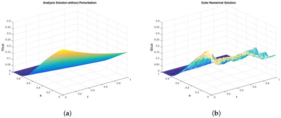
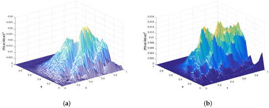
Figure 2. Sample paths produced by the square of the difference between (a) “explicit solution" $P(a,t)$ and (b) numerical solution $Q(a,t)$ under $\Delta t=0.005$ and $\Delta t=0.0005$, respectively (78).

In addition, it is not difficult to verify that system (78) has a unique invariant probability measure. However, for system (78), its true solution is almost impossible to find. Therefore, let the EM method generate the empirical distribution as the true invariant probability distribution. Inspired by [33], the statistic of the Kolmogorov–Smirnov test can be used to estimate the difference between two distributions. First, we choose 200 independent paths of (78) to simulate with $\Delta t=0.005$ from $t=0$ to $t=1$. We can easily obtain 10 paths after averaging at time $t=1$. The yellow line in Figure 3a describes the empirical distribution, which is constructed by 10 points at $t=1$. The blue line in Figure 3a represents the numerical invariant probability distribution generated by the EM method. The red line in Figure 3a shows that the error between the numerical invariant measure (i.e., numerical probability distribution) and the true invariant measure (i.e., true invariant probability distribution) gradually decreases with increasing time (t). Next, based on Figure 3, i.e., $W_p(\pi ,{\pi }^{\Delta }) \le C{\Delta }^{\frac{p}{2}}$, the log(error) plot of the differences between the numerical and true invariant probability distributions with step sizes is shown in Figure 3b. Obviously, it is not difficult to conclude that as the step size becomes smaller, the Wasserstein distance also decreases, tending toward 0.

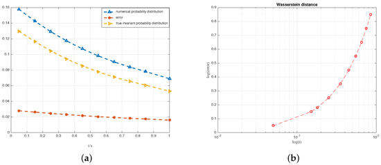
Figure 3. (a) The difference between the empirical and true distributions along the time line for system (78); (b) log–log plot of errors against step size.

5. Concluding Remarks

In this work, a class of stochastic age-dependent population–toxicant equations with Markovian switching was considered. Applying Gronwall inequality, a criterion for the existence and uniqueness of the invariant measure for the model was proposed. Moreover, we also proved the existence and uniqueness of the numerical invariance measure for system (3) when $\Delta$ is sufficiently small, and we proved that the numerical invariance measure converges at a rate of ${\Delta }^{\frac{p}{2}}$ to the invariance measure of the corresponding exact number. We outlined some possible research directions and problems for our future work. In this study, based on the classical population model [17,24], a stochastic age-dependent population model with Markov switching in a polluted environment was developed. The analysis was mathematical and methodological. In order to ensure the model moves closer to the biological background, a more realistic and simplified control equation is needed. The applications of the stochastic age-dependent population model with Markov switching will be the main research direction in our future work.

References

- Srinivasu, P.D.N. Control of environmental pollution to conserve a population. Nonlinear Anal. Real World Appl. 2002, 3, 397–411. [Google Scholar] [CrossRef]
- Amani, A.Z. Studies on the population dynamics of some common weeds under the stress of environmental pollution. J. Dent. 1983, 41, 195–206. [Google Scholar]
- Agarwal, M.; Devi, S. The effect of environmental tax on the survival of biological species in a polluted environment: A mathematical model. Nonlinear Anal. Model. Control 2010, 3, 271–286. [Google Scholar] [CrossRef]
- Hallam, T.G.; Clark, C.E.; Lassiter, R.R. Effects of toxicants on populations: A qualitative approach I. Equilibrium environmental exposure. Ecol. Model. 1983, 18, 291–304. [Google Scholar] [CrossRef]
- Hallam, T.G.; Clar, C.E.; Jordan, G.S. Effects of toxicant on population: A qualitative approach II. First Order Kinetics. J. Math. Biol. 1983, 109, 411–429. [Google Scholar] [CrossRef] [PubMed]
- Liu, H.; Ma, Z. The threshold of survival for system of two species in a polluted environment. J. Math. Biol. 1991, 30, 49–61. [Google Scholar] [PubMed]
- Feng, Y.; Wang, K. The survival analysis for single-species system in a polluted environment. Ann. Differ. Equ. 2006, 22, 154–159. [Google Scholar]
- Hallam, T.G.; Zhien, M. Persistence in Population models with demographic fluctuations. J. Math. Biol. 1986, 24, 327–339. [Google Scholar] [CrossRef] [PubMed]
- Jinxiao, P.; Zhen, J.; Zhien, M. Thresholds of survival for an n-dimensional Volterra mutualistic system in a polluted environment. J. Math. Anal. Appl. 2000, 252, 519–531. [Google Scholar] [CrossRef][Green Version]
- Mukherjee, D. Persistence and global stability of a population in a polluted environment with delay. J. Biol. Syst. 2008, 10, 225–232. [Google Scholar] [CrossRef]
- He, J.; Wang, K. The survival analysis for a population in a polluted environment. Nonlinear Anal. Real World Appl. 2009, 10, 1555–1571. [Google Scholar] [CrossRef]
- Li, R.; Leung, P.; Pang, W. Convergence of numerical solutions to stochastic age-dependent population equations with Markovian switching. J. Comput. Appl. Math. 2009, 233, 1046–1055. [Google Scholar] [CrossRef]
- Ma, W.; Zhang, Q. Convergence of the Semi-implicit Euler method for stochastic age-dependent population equations with Markovian switching. In Proceedings of the Information Computing and Applications, Tangshan, China, 15–18 October 2010; Springer: Berlin/Heidelberg, Germany, 2010. [Google Scholar]
- Rathinasamy, A. Split-step θ-methods for stochastic age-dependent population equations with Markovian switching. Nonlinear Anal. Real World Appl. 2012, 13, 1334–1345. [Google Scholar] [CrossRef]
- Liu, M.; Wang, K. Persistence and extinction of a stochastic single-species model under regime switching in a polluted environment II. J. Theor. Biol. 2010, 267, 283–291. [Google Scholar] [CrossRef]
- Yin, G.; Mao, X.; Yin, K. Numerical approximation of invariant measures for hybrid diffusion systems. IEEE Trans. Autom. Control 2005, 50, 934–946. [Google Scholar] [CrossRef]
- Bao, J.; Yin, G.; Yuan, C. Ergodicity for functional stochastic differential equations and applications. Nonlinear Anal. Theory Methods Appl. 2014, 98, 66–82. [Google Scholar] [CrossRef]
- Ruttanaprommarin, N.; Sabir, Z.; Núñez, R.A.S.; Az-Zobi, E.; Weera, W.; Botmart, T.; Zamart, C. A stochastic framework for solving the prey-predator delay differential model of Holling type-III. Comput. Mater. Contin. 2023, 3, 5915–5930. [Google Scholar] [CrossRef]
- Mao, X.; Yuan, C.; Yin, G. Numerical method for stationary distribution of stochastic differential equations with Markovian switching. J. Comput. Appl. Math. 2005, 174, 1–27. [Google Scholar] [CrossRef]
- Yu, X.; Yuan, S.; Zhang, T. Persistence and ergodicity of a stochastic single species model with Allee effect under regime switching. Commun. Nonlinear Sci. Numer. Simul. 2018, 59, 359–374. [Google Scholar] [CrossRef]
- Vassiliou, P.C.G. Non-Homogeneous Markov Chains and Systems. Theory and Applications; Chapman and Hall: London, UK; CRC Press: Boca Raton, FL, USA, 2023. [Google Scholar]
- Yuan, C.; Mao, X. Stationary distributions of Euler-Maruyama-type stochastic difference equations with Markovian switching and their convergence. J. Differ. Equ. Appl. 2005, 11, 29–48. [Google Scholar] [CrossRef]
- Bao, J.; Shao, J.; Yuan, C. Approximation of invariant measures for Regime-switching Diffusions. Potential Anal. 2016, 44, 707–727. [Google Scholar] [CrossRef]
- Zhao, Y.; Yuan, S.; Zhang, Q. Numerical solution of a fuzzy stochastic single-species age-structure model in a polluted environment. Appl. Math. Comput. 2015, 260, 385–396. [Google Scholar] [CrossRef]
- Wu, R.; Zou, X.; Wang, K. Dynamics of logistic systems driven by Lévy noise under regime switching. Electron. J. Differ. Equ. 2014, 2014, 1–16. [Google Scholar]
- Du, Y.; Ye, M.; Zhang, Q. A positivity-preserving numerical algorithm for stochastic age-dependent population system with Lévy noise in a polluted environment. Comput. Math. Appl. Int. J. 2022, 125, 51–79. [Google Scholar] [CrossRef]
- Mao, X.; Yuan, C. Stochastic Differential Equations with Markovian Switching; Imperial College Press: London, UK, 2006. [Google Scholar]
- Luo, Z.; Fan, X. Optimal control for an age-dependent competitive species model in a polluted environment. Appl. Math. Comput. 2014, 228, 91–101. [Google Scholar] [CrossRef]
- Yang, H.; Li, X. Explicit approximations for nonlinear switching diffusion systems in finite and infinite horizons. J. Differ. Equ. 2018, 265, 2921–2967. [Google Scholar] [CrossRef]
- Fu, X. On invariant measures and the asymptotic behavior of a stochastic delayed SIRS epidemic model. Phys. A 2019, 523, 1008–1023. [Google Scholar] [CrossRef]
- Mao, X. Stochastic Differential Equations and Applications, 2nd ed.; Horwood Publishing Limited: Chichester, UK, 2008. [Google Scholar]
- Anderson, W.J. Continuous-Time Markov Chains; Springer: Berlin/Heidelberg, Germany, 1991. [Google Scholar]
- Massey, F. The kolmogorov-smirnov test for goodness of fit. J. Am. Stat. Assoc. 1951, 46, 68–78. [Google Scholar] [CrossRef]
Disclaimer/Publisher’s Note: The statements, opinions and data contained in all publications are solely those of the individual author(s) and contributor(s) and not of MDPI and/or the editor(s). MDPI and/or the editor(s) disclaim responsibility for any injury to people or property resulting from any ideas, methods, instructions or products referred to in the content. |
© 2024 by the authors. Licensee MDPI, Basel, Switzerland. This article is an open access article distributed under the terms and conditions of the Creative Commons Attribution (CC BY) license (https://creativecommons.org/licenses/by/4.0/).