Optimal Control Applied to Piecewise-Fractional Ebola Model

Abstract

A recently proposed fractional-order mathematical model with Caputo derivatives was developed for Ebola disease. Here, we extend and generalize this model, beginning with its correction. A fractional optimal control (FOC) problem is then formulated and numerically solved with the rate of vaccination as the control measure. The research presented in this work addresses the problem of fitting real data from Guinea, Liberia, and Sierra Leone, available at the World Health Organization (WHO). A cost-effectiveness analysis is performed to assess the cost and effectiveness of the control measure during the intervention. We come to the conclusion that the fractional control is more efficient than the classical one only for a part of the time interval. Hence, we suggest a system where the derivative order changes over time, becoming fractional or classical when it makes more sense. This type of variable-order fractional model, known as piecewise derivative with fractional Caputo derivatives, is the most successful in managing the illness.

1. Introduction

Life begins with birth, growth follows, then multiplication, ageing, and has an end with death. Life consists of several stages. The transition between those stages makes life dynamic. It also depends on several conditions, such as food resources, natural resources, weather conditions, exposure to pathogen agents, etc. These are the ingredients of a compartmental model where differential equations manage transitions. In this work, we are interested in the dynamics of a population exposed to a particular microorganism, the Ebola virus.

Physical contact with body fluids, secretions, tissues, or semen from infected individuals can spread the highly pernicious Ebola virus [1,2]. Between 1976 and 2014, at least 18 Ebola outbreaks were confirmed in Africa. About 2400 cases and 1600 fatalities from the Ebola virus were reported up until 2012. On 27 March 2014, a new Ebola outbreak broke out in West Africa, resulting in 28,602 confirmed cases and 11,301 fatalities.

A few compartmental models of Ebola epidemics have recently been proposed [3,4,5,6,7,8,9,10]. A number of methods have been proposed to simulate the disease’s spread in three African nations—Guinea, Liberia, and Sierra Leone—affected by the 2014 outbreak. By including an additional variable for the quantity of vaccines, Ref. [4] addresses the optimal control problem of the Ebola epidemic with vaccination constraints. Fractional derivatives have been added to the models in a few studies [11,12]. A detailed study of an Ebola compartmental model with eight non-linear differential equations has also been proposed in [3].

A fractional order differential system has been employed recently to investigate the spread of Ebola [13]. That model is here generalised and the vaccination is here considered as a measure to control the infection. Conventional optimum control is generalized, and, as a result, fractional optimal control (FOC) is included. Unlike earlier studies, such as example [14], we were unable to identify a derivative order for which the fractional model fits data better than the classical model. We did find, nevertheless, that the fractional optimal control is more effective and is superior for a portion of the time interval. Therefore, we suggest a system in which the derivative order varies during the interval, becoming fractional or classical when it is more beneficial. This variable-order fractional system, named the piecewise fractional order derivative system, has been demonstrated to be helpful in the management of the illness.

The paper is organised as follows. The fractional order model formulation is presented in Section 2. The fractional optimal control of the model is depicted in Section 3. Main results are then given in Section 4: parameter estimation of the model (Section 4.1); numerical results and cost-effectiveness analysis for the fractional optimal control problem (Section 4.2); and the piecewise derivative with fractional Caputo derivatives (Section 4.2). Section 5 ends with conclusions and perspectives of future work.

2. The Fractional Order Model

A density-dependent demography of a dynamic population for Ebola disease [13], is considered. The compartmental model divided the total population N into 8 mutually exclusive compartments: susceptible (S), exposed (E), infected (I), asymptomatic but still infectious (R), dead but not buried (L), hospitalized (H), buried (B), and completely recovered (C). The Caputo fractional-order version of the model is given below.

$$\left\{\begin{array}{cc}\hfill { }_0^C{D}_t^{\alpha }S=& {\displaystyle ({\alpha }_1-{\alpha }_{2}N)N-\frac{{\beta }_i}{N}SI-\frac{{\beta }_h}{N}SH-\frac{{\beta }_d}{N}SL-\frac{{\beta }_r}{N}SR}\hfill \\ & -({\mu }_1+{\mu }_{2}N)S,\hfill \\ \hfill { }_0^C{D}_t^{\alpha }E=& {\displaystyle \frac{{\beta }_i}{N}SI+\frac{{\beta }_h}{N}SH+\frac{{\beta }_d}{N}SL+\frac{{\beta }_r}{N}SR-\sigma E-({\mu }_1+{\mu }_{2}N)E,}\hfill \\ \hfill { }_0^C{D}_t^{\alpha }I=& \sigma E-({\gamma }_1+\epsilon +\tau +{\mu }_1+{\mu }_{2}N)I,\hfill \\ \hfill { }_0^C{D}_t^{\alpha }R=& {\gamma }_{1}I+{\gamma }_{2}H-({\gamma }_3+{\mu }_1+{\mu }_{2}N)R,\hfill \\ \hfill { }_0^C{D}_t^{\alpha }L=& \epsilon I-({\delta }_1+\zeta )L,\hfill \\ \hfill { }_0^C{D}_t^{\alpha }H=& \tau I-({\gamma }_2+{\delta }_2+{\mu }_1+{\mu }_{2}N)H,\hfill \\ \hfill { }_0^C{D}_t^{\alpha }B=& {\delta }_{1}L+{\delta }_{2}H-\zeta B,\hfill \\ \hfill { }_0^C{D}_t^{\alpha }C=& {\gamma }_{3}R-({\mu }_1+{\mu }_{2}N)C.\hfill \end{array}\right..$$

(1)

where ${ }_0^C{D}_t^{\alpha }$ denotes the left Caputo fractional order derivative of order $\alpha$ ($0<\alpha <1$).

The time dimensions of the equations of model (1) are not appropriate. On the left-hand side, the dimension is (time)^α, while on the right-hand side, the dimension is (time)⁻¹. For more details, see [15,16], for instance. We claim that the proper way of writing system (1) is

$$\left\{\begin{array}{cc}\hfill { }_0^C{D}_t^{\alpha }S=& {\displaystyle ({\alpha }_1^{\alpha }-{\alpha }_2^{\alpha }N)N-\frac{{\beta }_i^{\alpha }}{N}SI-\frac{{\beta }_h^{\alpha }}{N}SH-\frac{{\beta }_d^{\alpha }}{N}SL-\frac{{\beta }_r^{\alpha }}{N}SR}\hfill \\ & -({\mu }_1^{\alpha }+{\mu }_2^{\alpha }N)S,\hfill \\ \hfill { }_0^C{D}_t^{\alpha }E=& {\displaystyle \frac{{\beta }_i^{\alpha }}{N}SI+\frac{{\beta }_h^{\alpha }}{N}SH+\frac{{\beta }_d^{\alpha }}{N}SL+\frac{{\beta }_r^{\alpha }}{N}SR-{\sigma }^{\alpha }E-({\mu }_1^{\alpha }+{\mu }_2^{\alpha }N)E,}\hfill \\ \hfill { }_0^C{D}_t^{\alpha }I=& {\sigma }^{\alpha }E-({\gamma }_1^{\alpha }+{\epsilon }^{\alpha }+{\tau }^{\alpha }+{\mu }_1^{\alpha }+{\mu }_2^{\alpha }N)I,\hfill \\ \hfill { }_0^C{D}_t^{\alpha }R=& {\gamma }_1^{\alpha }I+{\gamma }_2^{\alpha }H-({\gamma }_3^{\alpha }+{\mu }_1^{\alpha }+{\mu }_2^{\alpha }N)R,\hfill \\ \hfill { }_0^C{D}_t^{\alpha }L=& {\epsilon }^{\alpha }I-({\delta }_1^{\alpha }+{\zeta }^{\alpha })L,\hfill \\ \hfill { }_0^C{D}_t^{\alpha }H=& {\tau }^{\alpha }I-({\gamma }_2^{\alpha }+{\delta }_2^{\alpha }+{\mu }_1^{\alpha }+{\mu }_2^{\alpha }N)H,\hfill \\ \hfill { }_0^C{D}_t^{\alpha }B=& {\delta }_1^{\alpha }L+{\delta }_2^{\alpha }H-{\zeta }^{\alpha }B,\hfill \\ \hfill { }_0^C{D}_t^{\alpha }C=& {\gamma }_3^{\alpha }R-({\mu }_1^{\alpha }+{\mu }_2^{\alpha }N)C.\hfill \end{array}\right.$$

(2)

Following the steps of [13], and references cited therein, we obtain the basic reproduction number of model (2), that is

$$R_0=\frac{{\sigma }^{\alpha }({\beta }_i^{\alpha }{a}_1{a}_2{a}_3+a_3(a_1{\gamma }_1^{\alpha }+{\tau }^{\alpha }{\gamma }_2){\beta }_r^{\alpha }+a_1{a}_2{ϵ}^{\alpha }{\beta }_d^{\alpha }+a_2{a}_3{\tau }^{\alpha }{\beta }_h^{\alpha })}{a_1{a}_2{a}_3({\gamma }_1^{\alpha }+{ϵ}^{\alpha }+{\tau }^{\alpha }+a_4)({\sigma }^{\alpha }+a_4)}$$

(3)

with $a_1={\gamma }_1^{\alpha }+{\delta }_2^{\alpha }+{\mu }_1^{\alpha }+{\mu }_2^{\alpha }{N}^{\ast }$, $a_2={\gamma }_3+{\mu }_1^{\alpha }+{\mu }_2^{\alpha }{N}^{\ast }$, $a_3={\delta }_1^{\alpha }+{\xi }^{\alpha }$, $a_4={\mu }_1^{\alpha }+{\mu }_2^{\alpha }{N}^{\ast }$ and $N^{\ast }={\displaystyle \frac{{\alpha }_1^{\alpha }-{\mu }_1^{\alpha }}{{\alpha }_2^{\alpha }+{\mu }_2^{\alpha }}}$.

According to Figure 1, the variation of the derivative order, $\alpha$, influences the value of $R_0$. When the value of $\alpha$ is low and close to zero, the infection has no capability to spread to the population since $R_0<1$. However, when $\alpha$ surpasses 0.6, we observe that $R_0>1$, which means that the infection will be able to start spreading in the population. This last case needs attention from the health authorities and is the one that concerns us.

3. Fractional Optimal Control of the Model

We introduce in the fractional model (2), a control function $u\left(t\right)$, which represents the percentage of susceptible individuals being vaccinated at each instant of time t with $t\in [0,t_f]$. The resulting fractional optimal control problem consists in minimizing the objective function $\mathcal{J}$, that is, the cost associated with the vaccination programme, subject to controlled fractional dynamics. The mathematical formulation is

$$\begin{array}{c}\hfill \begin{array}{cc}\hfill min\mathcal{J}(I,& u)={\int }_0^{t_f}\left({\kappa }_{1}I+{\kappa }_2{u}^2\right)dt\hfill \\ \hfill \mathrm{s}\mathrm{u}\mathrm{b}\mathrm{j}\mathrm{e}\mathrm{c}\mathrm{t} \mathrm{t}\mathrm{o}\\ \hfill { }_0^C{D}_t^{\alpha }S=& {\displaystyle ({\alpha }_1^{\alpha }-{\alpha }_2^{\alpha }N)N-\frac{{\beta }_i^{\alpha }}{N}SI-\frac{{\beta }_h^{\alpha }}{N}SH-\frac{{\beta }_d^{\alpha }}{N}SL-\frac{{\beta }_r^{\alpha }}{N}SR}\hfill \\ \hfill & -({\mu }_1^{\alpha }+{\mu }_2^{\alpha }N+u^{\alpha })S,\hfill \\ \hfill { }_0^C{D}_t^{\alpha }E=& {\displaystyle \frac{{\beta }_i^{\alpha }}{N}SI+\frac{{\beta }_h^{\alpha }}{N}SH+\frac{{\beta }_d^{\alpha }}{N}SL+\frac{{\beta }_r^{\alpha }}{N}SR-\sigma E}\hfill \\ \hfill & -({\mu }_1^{\alpha }+{\mu }_2^{\alpha }N)E,\hfill \\ \hfill { }_0^C{D}_t^{\alpha }I=& {\sigma }^{\alpha }E-({\gamma }_1^{\alpha }+{\epsilon }^{\alpha }+{\tau }^{\alpha }+{\mu }_1^{\alpha }+{\mu }_2^{\alpha }N)I,\hfill \\ \hfill { }_0^C{D}_t^{\alpha }R=& {\gamma }_1^{\alpha }I+{\gamma }_2^{\alpha }H-({\gamma }_3^{\alpha }+{\mu }_1^{\alpha }+{\mu }_2^{\alpha }N)R,\hfill \\ \hfill { }_0^C{D}_t^{\alpha }L=& {\epsilon }^{\alpha }I-({\delta }_1^{\alpha }+{\zeta }^{\alpha })L,\hfill \\ \hfill { }_0^C{D}_t^{\alpha }H=& {\tau }^{\alpha }I-({\gamma }_2^{\alpha }+{\delta }_2^{\alpha }+{\mu }_1^{\alpha }+{\mu }_2^{\alpha }N)H,\hfill \\ \hfill { }_0^C{D}_t^{\alpha }B=& {\delta }_1^{\alpha }L+{\delta }_2^{\alpha }H-{\zeta }^{\alpha }B,\hfill \\ \hfill { }_0^C{D}_t^{\alpha }C=& {\gamma }_3^{\alpha }R-({\mu }_1^{\alpha }+{\mu }_2^{\alpha }N)C+u^{\alpha }S.\hfill \end{array}\end{array}$$

(4)

with given initial conditions

$$S\left(0\right),E\left(0\right),I\left(0\right),R\left(0\right),L\left(0\right),H\left(0\right),B\left(0\right),C\left(0\right)⩾0.$$

(5)

Parameters $0<{\kappa }_1,{\kappa }_2<+\infty$ are positive numbers that represent the weights associated with the number of infected individuals and on the cost associated with the vaccination program. The set of admissible control functions is

$$\mathcal{U}=\left\{u(·)\in L^{\infty }(0,t_f):0⩽u⩽u_{max}\right\}.$$

(6)

Since the integrand of the cost functional $\mathcal{J}$ is convex and the set of admissible control functions $\mathcal{U}$ is compact, we have by Filippov’s existence theorem (Theorem 3.1 of the reference [17]) that there exists at least one optimal control $\overline{u}$ and its associated optimal state trajectory $\overline{x}$. Pontryagin’s maximum principle (PMP) for fractional optimal control is used to determine the solution of the problem [17,18]. The Hamiltonian of the resulting optimal control problem is as follows:

$$\begin{array}{cc}\hfill H& ={\kappa }_{1}I+{\kappa }_2{u}^2+{\xi }_1(({\alpha }_1^{\alpha }-{\alpha }_2^{\alpha }N)N-\frac{{\beta }_i^{\alpha }}{N}SI-\frac{{\beta }_h^{\alpha }}{N}SH-\frac{{\beta }_d^{\alpha }}{N}SL-\frac{{\beta }_r^{\alpha }}{N}SR\hfill \\ \hfill & -({\mu }_1^{\alpha }+{\mu }_2^{\alpha }N+u^{\alpha })S)+{\xi }_2(\frac{{\beta }_i^{\alpha }}{N}SI+\frac{{\beta }_h^{\alpha }}{N}SH+\frac{{\beta }_d^{\alpha }}{N}SL+\frac{{\beta }_r^{\alpha }}{N}SR-{\sigma }^{\alpha }E\hfill \\ \hfill & -({\mu }_1^{\alpha }+{\mu }_2^{\alpha }N)E)+{\xi }_3({\sigma }^{\alpha }E-({\gamma }_1^{\alpha }+{\epsilon }^{\alpha }+{\tau }^{\alpha }+{\mu }_1^{\alpha }+{\mu }_2^{\alpha }N)I)+{\xi }_4({\gamma }_1^{\alpha }I+{\gamma }_2^{\alpha }H\hfill \\ \hfill & -({\gamma }_3^{\alpha }+{\mu }_1^{\alpha }+{\mu }_2^{\alpha }N)R)+{\xi }_5({\epsilon }^{\alpha }I-({\delta }_1^{\alpha }+{\zeta }^{\alpha })L)+{\xi }_6({\tau }^{\alpha }I-({\gamma }_2^{\alpha }+{\delta }_2^{\alpha }+{\mu }_1^{\alpha }\hfill \\ \hfill & +{\mu }_2^{\alpha }N\left)H\right)+{\xi }_7({\delta }_1^{\alpha }L+{\delta }_2^{\alpha }H-{\zeta }^{\alpha }B)+{\xi }_8({\gamma }_3^{\alpha }R-({\mu }_1^{\alpha }+{\mu }_2^{\alpha }N)C+u^{\alpha }S).\hfill \end{array}$$

(7)

The adjoint system asserts that the co-state variables ${\xi }_i\left(t\right),i=1,\dots ,8$, verify

$$\begin{array}{cc}\hfill { }_t{D}_{t_f}^{\alpha }{\xi }_1\left(t\right)=& I{\mu }_2^{\alpha }{\xi }_3+H{\mu }_2^{\alpha }{\xi }_6+{\mu }_2^{\alpha }{\xi }_{4}R-{\xi }_2(-E{\mu }_2^{\alpha }+\frac{{\beta }_h^{\alpha }H}{N}+\frac{{\beta }_i^{\alpha }I}{N}+\frac{{\beta }_d^{\alpha }L}{N}\hfill \\ \hfill & +\frac{{\beta }_r^{\alpha }R}{N}-\frac{{\beta }_h^{\alpha }HS}{N^2}-\frac{{\beta }_i^{\alpha }IS}{N^2}-\frac{{\beta }_d^{\alpha }LS}{N^2}-\frac{{\beta }_r^{\alpha }RS}{N^2})-{\xi }_1({\alpha }_1^{\alpha }-{\mu }_1^{\alpha }\hfill \\ \hfill & -\frac{{\beta }_h^{\alpha }H}{N}-\frac{{\beta }_i^{\alpha }I}{N}-\frac{{\beta }_d^{\alpha }L}{N}-2{\alpha }_2^{\alpha }N-{\mu }_2^{\alpha }N-\frac{{\beta }_r^{\alpha }R}{N}-{\mu }_2^{\alpha }S+\frac{{\beta }_h^{\alpha }HS}{N^2}\hfill \\ \hfill & +\frac{{\beta }_i^{\alpha }IS}{N^2}+\frac{{\beta }_d^{\alpha }LS}{N^2}+\frac{{\beta }_r^{\alpha }RS}{N^2}-u^{\alpha })+{\xi }_8(C{\mu }_2^{\alpha }-u^{\alpha }),\hfill \end{array}$$

(8)

$$\begin{array}{cc}\hfill { }_t{D}_{t_f}^{\alpha }{\xi }_2\left(t\right)=& H{\mu }_2^{\alpha }{\xi }_6+C{\mu }_2^{\alpha }{\xi }_8+{\mu }_2^{\alpha }{\xi }_{4}R-{\xi }_1({\alpha }_1^{\alpha }-2{\alpha }_2^{\alpha }N-{\mu }_2^{\alpha }S+\frac{{\beta }_h^{\alpha }HS}{N^2}\hfill \\ \hfill & +\frac{{\beta }_i^{\alpha }IS}{N^2}+\frac{{\beta }_d^{\alpha }LS}{N^2}+\frac{{\beta }_r^{\alpha }RS}{N^2})+{\xi }_2({\mu }_1^{\alpha }+E{\mu }_2^{\alpha }+{\mu }_2^{\alpha }N+\frac{{\beta }_h^{\alpha }HS}{N^2}\hfill \\ \hfill & +\frac{{\beta }_i^{\alpha }IS}{N^2}+\frac{{\beta }_d^{\alpha }LS}{N^2}+\frac{{\beta }_r^{\alpha }RS}{N^2}+{\sigma }^{\alpha })+{\xi }_3(I{\mu }_2^{\alpha }-{\sigma }^{\alpha }),\hfill \end{array}$$

(9)

$$\begin{array}{cc}\hfill { }_t{D}_{t_f}^{\alpha }{\xi }_3\left(t\right)=& -{\kappa }_1-{\epsilon }^{\alpha }{\xi }_5+C{\mu }_2^{\alpha }{\xi }_8-{\xi }_4({\gamma }_1^{\alpha }-{\mu }_2^{\alpha }R)+{\xi }_2(E{\mu }_2^{\alpha }+\frac{{\beta }_h^{\alpha }HS}{N^2}\hfill \\ \hfill & +\frac{{\beta }_i^{\alpha }IS}{N^2}+\frac{{\beta }_d^{\alpha }LS}{N^2}-\frac{{\beta }_i^{\alpha }S}{N}+\frac{{\beta }_r^{\alpha }RS}{N^2})-{\xi }_1({\alpha }_1^{\alpha }-2{\alpha }_2^{\alpha }N-{\mu }_2^{\alpha }S\hfill \\ \hfill & +\frac{{\beta }_h^{\alpha }HS}{N^2}+\frac{{\beta }_i^{\alpha }IS}{N^2}+\frac{{\beta }_d^{\alpha }LS}{N^2}-\frac{{\beta }_i^{\alpha }S}{N}+\frac{{\beta }_r^{\alpha }RS}{N^2})-{\xi }_3(-{\epsilon }^{\alpha }-{\gamma }_1^{\alpha }-{\mu }_1^{\alpha }\hfill \\ \hfill & -I{\mu }_2^{\alpha }-{\mu }_2^{\alpha }N-{\tau }^{\alpha })+{\xi }_6(H{\mu }_2^{\alpha }-{\tau }^{\alpha }),\hfill \end{array}$$

(10)

$$\begin{array}{cc}\hfill { }_t{D}_{t_f}^{\alpha }{\xi }_4\left(t\right)=& I{\mu }_2^{\alpha }{\xi }_3+H{\mu }_2^{\alpha }{\xi }_6-({\gamma }_3^{\alpha }-C{\mu }_2^{\alpha }){\xi }_8+{\xi }_4({\gamma }_3^{\alpha }+{\mu }_1^{\alpha }+{\mu }_2^{\alpha }N+{\mu }_2^{\alpha }R)\hfill \\ \hfill & +{\xi }_2\left(E{\mu }_2^{\alpha }+\frac{{\beta }_h^{\alpha }HS}{N^2}+\frac{{\beta }_i^{\alpha }IS}{N^2}+\frac{{\beta }_d^{\alpha }LS}{N^2}-\frac{{\beta }_r^{\alpha }S}{N}+\frac{{\beta }_r^{\alpha }RS}{N^2}\right)-{\xi }_1({\alpha }_1^{\alpha }\hfill \\ \hfill & -2{\alpha }_2^{\alpha }N-{\mu }_2^{\alpha }S+\frac{{\beta }_h^{\alpha }HS}{N^2}+\frac{{\beta }_i^{\alpha }IS}{N^2}+\frac{{\beta }_d^{\alpha }LS}{N^2}-\frac{{\beta }_r^{\alpha }S}{N}+\frac{{\beta }_r^{\alpha }RS}{N^2}),\hfill \end{array}$$

(11)

$$\begin{array}{cc}\hfill { }_t{D}_{t_f}^{\alpha }{\xi }_5\left(t\right)=& I{\mu }_2^{\alpha }{\xi }_3+({\zeta }^{\alpha }+{\delta }_1^{\alpha }){\xi }_5+H{\mu }_2^{\alpha }{\xi }_6-{\delta }_1^{\alpha }{\xi }_7+C{\mu }_2^{\alpha }{\xi }_8+{\mu }_2^{\alpha }{\xi }_{4}R+{\xi }_2(E{\mu }_2^{\alpha }\hfill \\ \hfill & +\frac{{\beta }_h^{\alpha }HS}{N^2}+\frac{{\beta }_i^{\alpha }IS}{N^2}+\frac{{\beta }_d^{\alpha }LS}{N^2}-\frac{{\beta }_d^{\alpha }S}{N}+\frac{{\beta }_r^{\alpha }RS}{N^2})-{\xi }_1({\alpha }_1^{\alpha }-2{\alpha }_2^{\alpha }N\hfill \end{array}$$

(12)

$$\begin{array}{c}\hfill -{\mu }_2^{\alpha }S+\frac{{\beta }_h^{\alpha }HS}{N^2}+\frac{{\beta }_i^{\alpha }IS}{N^2}+\frac{{\beta }_d^{\alpha }LS}{N^2}-\frac{{\beta }_d^{\alpha }S}{N}+\frac{{\beta }_r^{\alpha }RS}{N^2}),\end{array}$$

$$\begin{array}{cc}\hfill { }_t{D}_{t_f}^{\alpha }{\xi }_6\left(t\right)=& I{\mu }_2^{\alpha }{\xi }_3+({\delta }_2^{\alpha }+{\gamma }_2^{\alpha }+{\mu }_1^{\alpha }+H{\mu }_2^{\alpha }+{\mu }_2^{\alpha }N){\xi }_6-{\delta }_2^{\alpha }{\xi }_7+C{\mu }_2^{\alpha }{\xi }_8-{\xi }_4({\gamma }_2^{\alpha }\hfill \\ \hfill & -{\mu }_2^{\alpha }R)+{\xi }_2\left(E{\mu }_2^{\alpha }+\frac{{\beta }_h^{\alpha }HS}{N^2}+\frac{{\beta }_i^{\alpha }IS}{N^2}+\frac{{\beta }_d^{\alpha }LS}{N^2}-\frac{{\beta }_h^{\alpha }S}{N}+\frac{{\beta }_r^{\alpha }RS}{N^2}\right)\hfill \\ \hfill & -{\xi }_1({\alpha }_1^{\alpha }-2{\alpha }_2^{\alpha }N-{\mu }_2^{\alpha }S+\frac{{\beta }_h^{\alpha }HS}{N^2}+\frac{{\beta }_i^{\alpha }IS}{N^2}+\frac{{\beta }_d^{\alpha }LS}{N^2}-\frac{{\beta }_h^{\alpha }S}{N}\hfill \\ \hfill & +\frac{{\beta }_r^{\alpha }RS}{N^2})\hfill \end{array}$$

(13)

$$\begin{array}{cc}\hfill { }_t{D}_{t_f}^{\alpha }{\xi }_7\left(t\right)=& I{\mu }_2^{\alpha }{\xi }_3+H{\mu }_2^{\alpha }{\xi }_6+{\zeta }^{\alpha }{\xi }_7+C{\mu }_2^{\alpha }{\xi }_8+{\mu }_2^{\alpha }{\xi }_{4}R+{\xi }_2(E{\mu }_2^{\alpha }+\frac{{\beta }_h^{\alpha }HS}{N^2}\hfill \\ \hfill & +\frac{{\beta }_i^{\alpha }IS}{N^2}+\frac{{\beta }_d^{\alpha }LS}{N^2}+\frac{{\beta }_r^{\alpha }RS}{N^2})-{\xi }_1({\alpha }_1^{\alpha }-2{\alpha }_2^{\alpha }N-{\mu }_2^{\alpha }S+\frac{{\beta }_h^{\alpha }HS}{N^2}\hfill \\ \hfill & +\frac{{\beta }_i^{\alpha }IS}{N^2}+\frac{{\beta }_d^{\alpha }LS}{N^2}+\frac{{\beta }_r^{\alpha }RS}{N^2})\hfill \end{array}$$

(14)

$$\begin{array}{cc}\hfill { }_t{D}_{t_f}^{\alpha }{\xi }_8\left(t\right)=& I{\mu }_2^{\alpha }{\xi }_3+H{\mu }_2^{\alpha }{\xi }_6+({\mu }_1^{\alpha }+C{\mu }_2^{\alpha }+{\mu }_2^{\alpha }N){\xi }_8+{\mu }_2^{\alpha }{\xi }_{4}R+{\xi }_2(E{\mu }_2^{\alpha }\hfill \\ \hfill & +\frac{{\beta }_h^{\alpha }HS}{N^2}+\frac{{\beta }_i^{\alpha }IS}{N^2}+\frac{{\beta }_d^{\alpha }LS}{N^2}+\frac{{\beta }_r^{\alpha }RS}{N^2})-{\xi }_1({\alpha }_1^{\alpha }-2{\alpha }_2^{\alpha }N-{\mu }_2^{\alpha }S\hfill \\ \hfill & +\frac{{\beta }_h^{\alpha }HS}{N^2}+\frac{{\beta }_i^{\alpha }IS}{N^2}+\frac{{\beta }_d^{\alpha }LS}{N^2}+\frac{{\beta }_r^{\alpha }RS}{N^2})\hfill \end{array}$$

(15)

which is a fractional system of right Riemann–Liouville derivatives, ${ }_t{D}_{t_f}^{\alpha }$ (see, e.g., [19]).

In turn, the optimality conditions of PMP establish that the optimal control $u^{\ast }$ is defined by

$$\begin{array}{cc}\hfill u& =min\left\{max\left\{0,{\left(\frac{\alpha ({\xi }_1-{\xi }_8)S}{2{\kappa }_2}\right)}^{\frac{1}{2-\alpha }}\right\},u_{max}\right\}.\hfill \end{array}$$

(16)

In addition, the following transversality conditions hold:

$${\xi }_1\left(t_f\right)={\xi }_2\left(t_f\right)=\dots ={\xi }_8\left(t_f\right)=0.$$

(17)

Let us apply the following change of variable

$$t^{\prime }=t_f-t$$

to the adjoint system (8)–(15) and to the transversality conditions (17). As a consequence, they are transformed into a left Riemann–Liouville fractional initial value problem:

$$\begin{array}{cc}\hfill { }_0{D}_{t^{\prime }}^{\alpha }{\xi }_1\left(t^{\prime }\right)=& -[I{\mu }_2^{\alpha }{\xi }_3+H{\mu }_2^{\alpha }{\xi }_6+{\mu }_2^{\alpha }{\xi }_{4}R-{\xi }_2(-E{\mu }_2^{\alpha }+\frac{{\beta }_h^{\alpha }H}{N}+\frac{{\beta }_i^{\alpha }I}{N}+\frac{{\beta }_d^{\alpha }L}{N}\hfill \\ \hfill & +\frac{{\beta }_r^{\alpha }R}{N}-\frac{{\beta }_h^{\alpha }HS}{N^2}-\frac{{\beta }_i^{\alpha }IS}{N^2}-\frac{{\beta }_d^{\alpha }LS}{N^2}-\frac{{\beta }_r^{\alpha }RS}{N^2})-{\xi }_1({\alpha }_1^{\alpha }-{\mu }_1^{\alpha }\hfill \\ \hfill & -\frac{{\beta }_h^{\alpha }H}{N}-\frac{{\beta }_i^{\alpha }I}{N}-\frac{{\beta }_d^{\alpha }L}{N}-2{\alpha }_2^{\alpha }N-{\mu }_2^{\alpha }N-\frac{{\beta }_r^{\alpha }R}{N}-{\mu }_2^{\alpha }S+\frac{{\beta }_h^{\alpha }HS}{N^2}\hfill \\ \hfill & +\frac{{\beta }_i^{\alpha }IS}{N^2}+\frac{{\beta }_d^{\alpha }LS}{N^2}+\frac{{\beta }_r^{\alpha }RS}{N^2}-u^{\alpha })+{\xi }_8(C{\mu }_2^{\alpha }-u^{\alpha })],\hfill \end{array}$$

(18)

$$\begin{array}{cc}\hfill { }_0{D}_{t^{\prime }}^{\alpha }{\xi }_2\left(t^{\prime }\right)=& -[H{\mu }_2^{\alpha }{\xi }_6+C{\mu }_2^{\alpha }{\xi }_8+{\mu }_2^{\alpha }{\xi }_{4}R-{\xi }_1({\alpha }_1^{\alpha }-2{\alpha }_2^{\alpha }N-{\mu }_2^{\alpha }S+\frac{{\beta }_h^{\alpha }HS}{N^2}\hfill \\ \hfill & +\frac{{\beta }_i^{\alpha }IS}{N^2}+\frac{{\beta }_d^{\alpha }LS}{N^2}+\frac{{\beta }_r^{\alpha }RS}{N^2})+{\xi }_2({\mu }_1^{\alpha }+E{\mu }_2^{\alpha }+{\mu }_2^{\alpha }N+\frac{{\beta }_h^{\alpha }HS}{N^2}\hfill \\ \hfill & +\frac{{\beta }_i^{\alpha }IS}{N^2}+\frac{{\beta }_d^{\alpha }LS}{N^2}+\frac{{\beta }_r^{\alpha }RS}{N^2}+{\sigma }^{\alpha })+{\xi }_3(I{\mu }_2^{\alpha }-{\sigma }^{\alpha })],\hfill \end{array}$$

(19)

$$\begin{array}{cc}\hfill { }_0{D}_{t^{\prime }}^{\alpha }{\xi }_3\left(t^{\prime }\right)=& -[-{\kappa }_1-{\epsilon }^{\alpha }{\xi }_5+C{\mu }_2^{\alpha }{\xi }_8-{\xi }_4({\gamma }_1^{\alpha }-{\mu }_2^{\alpha }R)+{\xi }_2(E{\mu }_2^{\alpha }+\frac{{\beta }_h^{\alpha }HS}{N^2}\hfill \\ \hfill & +\frac{{\beta }_i^{\alpha }IS}{N^2}+\frac{{\beta }_d^{\alpha }LS}{N^2}-\frac{{\beta }_i^{\alpha }S}{N}+\frac{{\beta }_r^{\alpha }RS}{N^2})-{\xi }_1({\alpha }_1^{\alpha }-2{\alpha }_2^{\alpha }N-{\mu }_2^{\alpha }S\hfill \\ \hfill & +\frac{{\beta }_h^{\alpha }HS}{N^2}+\frac{{\beta }_i^{\alpha }IS}{N^2}+\frac{{\beta }_d^{\alpha }LS}{N^2}-\frac{{\beta }_i^{\alpha }S}{N}+\frac{{\beta }_r^{\alpha }RS}{N^2})-{\xi }_3(-{\epsilon }^{\alpha }-{\gamma }_1^{\alpha }-{\mu }_1^{\alpha }\hfill \\ \hfill & -I{\mu }_2^{\alpha }-{\mu }_2^{\alpha }N-{\tau }^{\alpha })+{\xi }_6(H{\mu }_2^{\alpha }-{\tau }^{\alpha })],\hfill \end{array}$$

(20)

$$\begin{array}{cc}\hfill { }_0{D}_{t^{\prime }}^{\alpha }{\xi }_4\left(t^{\prime }\right)=& -[I{\mu }_2^{\alpha }{\xi }_3+H{\mu }_2^{\alpha }{\xi }_6-({\gamma }_3^{\alpha }-C{\mu }_2^{\alpha }){\xi }_8+{\xi }_4({\gamma }_3^{\alpha }+{\mu }_1^{\alpha }+{\mu }_2^{\alpha }N+{\mu }_2^{\alpha }R)\hfill \\ \hfill & +{\xi }_2\left(E{\mu }_2^{\alpha }+\frac{{\beta }_h^{\alpha }HS}{N^2}+\frac{{\beta }_i^{\alpha }IS}{N^2}+\frac{{\beta }_d^{\alpha }LS}{N^2}-\frac{{\beta }_r^{\alpha }S}{N}+\frac{{\beta }_r^{\alpha }RS}{N^2}\right)-{\xi }_1({\alpha }_1^{\alpha }\hfill \\ \hfill & -2{\alpha }_2^{\alpha }N-{\mu }_2^{\alpha }S+\frac{{\beta }_h^{\alpha }HS}{N^2}+\frac{{\beta }_i^{\alpha }IS}{N^2}+\frac{{\beta }_d^{\alpha }LS}{N^2}-\frac{{\beta }_r^{\alpha }S}{N}+\frac{{\beta }_r^{\alpha }RS}{N^2}\left)\right],\hfill \end{array}$$

(21)

$$\begin{array}{cc}\hfill { }_t{D}_{t_f}^{\alpha }{\xi }_5\left(t\right)=& -[I{\mu }_2^{\alpha }{\xi }_3+({\zeta }^{\alpha }+{\delta }_1^{\alpha }){\xi }_5+H{\mu }_2^{\alpha }{\xi }_6-{\delta }_1^{\alpha }{\xi }_7+C{\mu }_2^{\alpha }{\xi }_8+{\mu }_2^{\alpha }{\xi }_{4}R+{\xi }_2(E{\mu }_2^{\alpha }\hfill \\ \hfill & +\frac{{\beta }_h^{\alpha }HS}{N^2}+\frac{{\beta }_i^{\alpha }IS}{N^2}+\frac{{\beta }_d^{\alpha }LS}{N^2}-\frac{{\beta }_d^{\alpha }S}{N}+\frac{{\beta }_r^{\alpha }RS}{N^2})-{\xi }_1({\alpha }_1^{\alpha }-2{\alpha }_2^{\alpha }N\hfill \\ \hfill & -{\mu }_2^{\alpha }S+\frac{{\beta }_h^{\alpha }HS}{N^2}+\frac{{\beta }_i^{\alpha }IS}{N^2}+\frac{{\beta }_d^{\alpha }LS}{N^2}-\frac{{\beta }_d^{\alpha }S}{N}+\frac{{\beta }_r^{\alpha }RS}{N^2}\left)\right],\hfill \end{array}$$

(22)

$$\begin{array}{cc}\hfill { }_0{D}_{t^{\prime }}^{\alpha }{\xi }_6\left(t^{\prime }\right)=& -[I{\mu }_2^{\alpha }{\xi }_3+({\delta }_2^{\alpha }+{\gamma }_2^{\alpha }+{\mu }_1^{\alpha }+H{\mu }_2^{\alpha }+{\mu }_2^{\alpha }N){\xi }_6-{\delta }_2^{\alpha }{\xi }_7+C{\mu }_2^{\alpha }{\xi }_8-{\xi }_4({\gamma }_2^{\alpha }\hfill \\ \hfill & -{\mu }_2^{\alpha }R)+{\xi }_2\left(E{\mu }_2^{\alpha }+\frac{{\beta }_h^{\alpha }HS}{N^2}+\frac{{\beta }_i^{\alpha }IS}{N^2}+\frac{{\beta }_d^{\alpha }LS}{N^2}-\frac{{\beta }_h^{\alpha }S}{N}+\frac{{\beta }_r^{\alpha }RS}{N^2}\right)\hfill \\ \hfill & -{\xi }_1({\alpha }_1^{\alpha }-2{\alpha }_2^{\alpha }N-{\mu }_2^{\alpha }S+\frac{{\beta }_h^{\alpha }HS}{N^2}+\frac{{\beta }_i^{\alpha }IS}{N^2}+\frac{{\beta }_d^{\alpha }LS}{N^2}-\frac{{\beta }_h^{\alpha }S}{N}\hfill \\ \hfill & +\frac{{\beta }_r^{\alpha }RS}{N^2}\left)\right]\hfill \end{array}$$

(23)

$$\begin{array}{cc}\hfill { }_0{D}_{t^{\prime }}^{\alpha }{\xi }_7\left(t^{\prime }\right)=& -[I{\mu }_2^{\alpha }{\xi }_3+H{\mu }_2^{\alpha }{\xi }_6+{\zeta }^{\alpha }{\xi }_7+C{\mu }_2^{\alpha }{\xi }_8+{\mu }_2^{\alpha }{\xi }_{4}R+{\xi }_2(E{\mu }_2^{\alpha }+\frac{{\beta }_h^{\alpha }HS}{N^2}\hfill \\ \hfill & +\frac{{\beta }_i^{\alpha }IS}{N^2}+\frac{{\beta }_d^{\alpha }LS}{N^2}+\frac{{\beta }_r^{\alpha }RS}{N^2})-{\xi }_1({\alpha }_1^{\alpha }-2{\alpha }_2^{\alpha }N-{\mu }_2^{\alpha }S+\frac{{\beta }_h^{\alpha }HS}{N^2}\hfill \\ \hfill & +\frac{{\beta }_i^{\alpha }IS}{N^2}+\frac{{\beta }_d^{\alpha }LS}{N^2}+\frac{{\beta }_r^{\alpha }RS}{N^2}\left)\right]\hfill \end{array}$$

(24)

$$\begin{array}{cc}\hfill { }_0{D}_{t^{\prime }}^{\alpha }{\xi }_8\left(t^{\prime }\right)=& -[I{\mu }_2^{\alpha }{\xi }_3+H{\mu }_2^{\alpha }{\xi }_6+({\mu }_1^{\alpha }+C{\mu }_2^{\alpha }+{\mu }_2^{\alpha }N){\xi }_8+{\mu }_2^{\alpha }{\xi }_{4}R+{\xi }_2(E{\mu }_2^{\alpha }\hfill \\ \hfill & +\frac{{\beta }_h^{\alpha }HS}{N^2}+\frac{{\beta }_i^{\alpha }IS}{N^2}+\frac{{\beta }_d^{\alpha }LS}{N^2}+\frac{{\beta }_r^{\alpha }RS}{N^2})-{\xi }_1({\alpha }_1^{\alpha }-2{\alpha }_2^{\alpha }N-{\mu }_2^{\alpha }S\hfill \\ \hfill & +\frac{{\beta }_h^{\alpha }HS}{N^2}+\frac{{\beta }_i^{\alpha }IS}{N^2}+\frac{{\beta }_d^{\alpha }LS}{N^2}+\frac{{\beta }_r^{\alpha }RS}{N^2}\left)\right]\hfill \\ \hfill \end{array}$$

(25)

with initial conditions:

$${\xi }_i\left(t^{\prime }\right){|}_{\begin{array}{c}{t}^{\prime }=0\end{array}}=0,i=1,\dots ,8.$$

(26)

Condition (26) implies that

$${ }_0{D}_{t^{\prime }}^{\alpha }{\xi }_i\left(t^{\prime }\right)={ }_0^C{D}_{t^{\prime }}^{\alpha }{\xi }_i\left(t^{\prime }\right),i=1,\dots ,8,$$

meaning that the adjoint system (18)–(15) can be considered a Caputo system of fractional differential equations (see, e.g., ([18] Section 3.3)).

4. Main Results

Our first step is to examine the degree of realism of the model, covered in Section 2, in relation to Ebola using real data from Guinea, Liberia, and Sierra Leone obtained from WHO. For that purpose, we need to accurately estimate some of the parameter values.

4.1. Parameter Estimation

In model fitting, the values of several parameters of the model were obtained from the literature and are presented in Table 1. The initial conditions are stated in Table 2.

The model was fitted to data on the cumulative confirmed cases from day 4 to 438, including an abrupt increase from 5666 to 7206 in days 212–216. This jump has an impact on fitting. The data were obtained from the WHO. Our results are given in Figure 2.

The fitted values for selected parameters of the model are displayed in Table 3 along with the root mean square deviation (RMSD), for two values of derivative order, such that

$$\mathrm{RMSD}(x,\widehat{x})=\sqrt{\frac{1}{n}\sum _{i=1}^n{(x_i-{\widehat{x}}_i)}^2}$$

where n is the total number of data points, $\widehat{x}$ represents estimated values, and x represents real values. Fitting was performed by adjusting the parameter values iteratively to improve the fit between model predictions and observed data. This was the fitting method. The two values considered for derivative order correspond to the classical model and to the fractional order model with the lowest value of RMSD. The difference between the two models is rather small and does not justify the replacement of the classical model by the pure fractional model.

Table 1. A complete list of detailed parameters, the correspondent values of some of them, and bibliographic sources.

Parameter	Value	Description	Source
${\alpha }_1$	0.03537	Density-independent part of the birth rate for individuals.	[13]
${\alpha }_2$	–	Density-dependent part of the birth rate for individuals.
${\beta }_i$	0.14	Contact rate of infective individuals and susceptible.	[4]
${\beta }_h$	0.29	Contact rate of infective individuals and hospitalized.	[4]
${\beta }_d$	0.40	Contact rate of infective individuals and dead.	[4]
${\beta }_r$	–	Contact rate of infective individuals and asymptomatic.
$\sigma$	1/11.4	Per capita rate at which exposed individuals become infectious.	[4]
${\gamma }_1$	1/10	Per capita rate of progression of individuals from the infectious class to the asymptomatic class.	[4]
${\gamma }_2$	1/5	Per capita rate of progression of individuals from the hospitalized class to the asymptomatic class.	[4]
${\gamma }_3$	1/30	Per capita recovery rate of individuals from the asymptomatic class to the complete recovered class.	[4]
$\epsilon$	1/9.6	Fatality rate.	[4]
$\tau$	0.2	Per capita rate of progression of individuals from the infectious class to the hospitalized class.	[4]
$\xi$	$14\times {10}^{-3}$	incineration rate	[4]
${\delta }_1$	0.5	Per capita rate of progression of individuals from the dead class to the buried class.	[4]
${\delta }_2$	1/4.6	Per capita rate of progression of individuals from the hospitalized class to the buried class.	[4]
${\mu }_1$	$1.017\times {10}^{-4}$	Density independent part of the death rate for individuals.	[13]
${\mu }_2$	–	Density dependent part of the death rate for individuals.

Table 1. A complete list of detailed parameters, the correspondent values of some of them, and bibliographic sources.

Parameter	Value	Description	Source
${\alpha }_1$	0.03537	Density-independent part of the birth rate for individuals.	[13]
${\alpha }_2$	–	Density-dependent part of the birth rate for individuals.
${\beta }_i$	0.14	Contact rate of infective individuals and susceptible.	[4]
${\beta }_h$	0.29	Contact rate of infective individuals and hospitalized.	[4]
${\beta }_d$	0.40	Contact rate of infective individuals and dead.	[4]
${\beta }_r$	–	Contact rate of infective individuals and asymptomatic.
$\sigma$	1/11.4	Per capita rate at which exposed individuals become infectious.	[4]
${\gamma }_1$	1/10	Per capita rate of progression of individuals from the infectious class to the asymptomatic class.	[4]
${\gamma }_2$	1/5	Per capita rate of progression of individuals from the hospitalized class to the asymptomatic class.	[4]
${\gamma }_3$	1/30	Per capita recovery rate of individuals from the asymptomatic class to the complete recovered class.	[4]
$\epsilon$	1/9.6	Fatality rate.	[4]
$\tau$	0.2	Per capita rate of progression of individuals from the infectious class to the hospitalized class.	[4]
$\xi$	$14\times {10}^{-3}$	incineration rate	[4]
${\delta }_1$	0.5	Per capita rate of progression of individuals from the dead class to the buried class.	[4]
${\delta }_2$	1/4.6	Per capita rate of progression of individuals from the hospitalized class to the buried class.	[4]
${\mu }_1$	$1.017\times {10}^{-4}$	Density independent part of the death rate for individuals.	[13]
${\mu }_2$	–	Density dependent part of the death rate for individuals.

Table 2. Initial conditions for the fractional optimal control problem: integer values closest to the endemic equilibrium of a fractional Ebola model with a derivative order of $\alpha =0.99993$.

$\mathit{S}\left(0\right)$	$\mathit{E}\left(0\right)$	$\mathit{I}\left(0\right)$	$\mathit{R}\left(0\right)$	$\mathit{L}\left(0\right)$	$\mathit{H}\left(0\right)$	$\mathit{B}\left(0\right)$	$\mathit{C}\left(0\right)$
31,329	3295	663	1923	134	295	9378	2013

Table 2. Initial conditions for the fractional optimal control problem: integer values closest to the endemic equilibrium of a fractional Ebola model with a derivative order of $\alpha =0.99993$.

$\mathit{S}\left(0\right)$	$\mathit{E}\left(0\right)$	$\mathit{I}\left(0\right)$	$\mathit{R}\left(0\right)$	$\mathit{L}\left(0\right)$	$\mathit{H}\left(0\right)$	$\mathit{B}\left(0\right)$	$\mathit{C}\left(0\right)$
31,329	3295	663	1923	134	295	9378	2013

Figure 2. Fitting the real data with the model.

Figure 2. Fitting the real data with the model.

Table 3. Fitted parameters of the model and the correspondent RMSD error.

			RMSD
${\mathbf{\beta }}_{\mathbf{r}}$	${\mathbf{\alpha }}_{\mathbf{2}}$	${\mathbf{\mu }}_{\mathbf{2}}$	$\mathbf{\alpha }=\mathbf{1}.\mathbf{0}$	$\mathbf{\alpha }=\mathbf{0}.\mathbf{99993}$
$1.9996\times {10}^{-1}$	$1.424378\times {10}^{-7}$	$6.468607\times {10}^{-7}$	306.69	306.476

Table 3. Fitted parameters of the model and the correspondent RMSD error.

			RMSD
${\mathbf{\beta }}_{\mathbf{r}}$	${\mathbf{\alpha }}_{\mathbf{2}}$	${\mathbf{\mu }}_{\mathbf{2}}$	$\mathbf{\alpha }=\mathbf{1}.\mathbf{0}$	$\mathbf{\alpha }=\mathbf{0}.\mathbf{99993}$
$1.9996\times {10}^{-1}$	$1.424378\times {10}^{-7}$	$6.468607\times {10}^{-7}$	306.69	306.476

4.2. Numerical Results and Cost-Effectiveness Analysis for the Fractional Optimal Control Problem

The predict–evaluate–correct–evaluate (PECE) method of Adams–Basforth–Moulton [20], which we implemented in MATLAB, is used to numerically solve the optimal control problem, as explained in Section 3, both in classical and fractional cases. The convergence of PECE’s method can be found in [21], and it has a global error of order two [22]. This approach applies the Pontryagin Maximum Principle. The forward–backward method given in this work generalizes the technique proposed in reference [23].

First, we use the PECE approach to solve systems (4) and (5). We use Table 2’s initial values for the state variables and an estimate for the control over the interval $[0,t_f]$ to determine the state variables’ values. The fractional initial value problem (IVP) (18)–() is obtained by applying a change of variable to the adjoint system and the transversality conditions. The values of the co-state variables ${\xi }_i,i=1,\dots ,8$, are found by solving this IVP using the PECE algorithm as well. After that, the control is updated using a convex combination of the current values and the control from the previous iteration, calculated in accordance with (16). This process is carried out repeatedly until all variable values and control values are almost the same as the previous iteration. A classical forward–backward technique, which we also developed in MATLAB, correctly corroborated the solutions of the classical model.

The weights of the cost functional (4) balance the relative importance of control terms. In this particular case, we consider that the weights are ${\kappa }_1={\kappa }_2=1$.

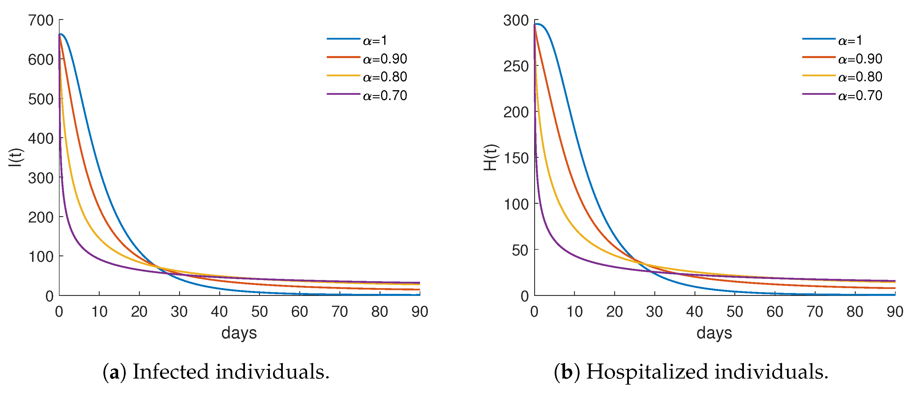
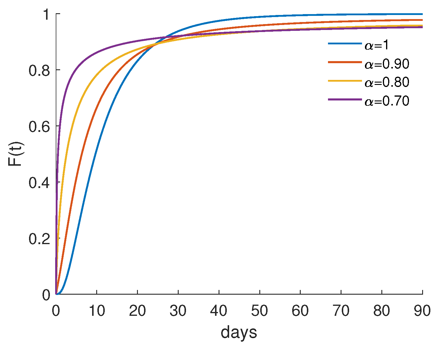
Without loss of generality, we consider the fractional order derivatives $\alpha =1.0$, $0.9$, $0.8$, and $0.7$. The solutions to the fractional optimal control problem for those values of $\alpha$ are displayed in Figure 3 and Figure 4. A change in the value of $\alpha$ corresponds to significant variations of the state and control variables. Additionally, in Figure 4 we observe that the graphic of the control variable u for the considered lowest value of $\alpha$ is clearly different from the other graphics. In all presented cases, we see that vaccination starts at maximum strength and reduces to zero at the end of the treatment period.

The efficacy of intervention is measured through a function [24] whose graphics are shown in Figure 5 and is defined as

$$F\left(t\right)=\frac{I\left(0\right)-I^{\ast }\left(t\right)}{I\left(0\right)}=1-\frac{I^{\ast }\left(t\right)}{I\left(0\right)},$$

(27)

where $I^{\ast }\left(t\right)$ is the optimal solution associated to the fractional optimal control problem, and $I\left(0\right)$ is the correspondent’s initial condition. This function measures the proportional variation in the number of infected individuals after the application of the vaccination (control), by comparing the number of infectious individuals at a given time t with its initial value $I\left(0\right)$. We can see that the graphic of $F\left(t\right)$ exhibits the inverse behaviour of the infected individuals curve, always growing, and reach their maximum at the end of the time interval.

Some summary measures are then presented to assess the cost and effectiveness of the proposed fractional control measure during the intervention period. For more details about these measures, see references [24,25]. The total cases averted by the intervention during the stipulated time period $t_f$ is defined by

$$AV=t_{f}I\left(0\right)-{\int }_0^{t_f}{I}^{\ast }\left(t\right)dt,$$

(28)

where $I^{\ast }\left(t\right)$ is the optimal solution given by the fractional optimal control and $I\left(0\right)$ is the correspondent initial condition. Note that this initial condition is obtained as the equilibrium proportion $\overline{I}$ of system (2), which is independent of time, so that ${\displaystyle t_{f}I\left(0\right)={\int }_0^{t_f}\overline{I}dt}$ represents the total infectious cases over a given period of $t_f$ days.

Effectiveness is determined by the proportion of cases averted from the total possible cases under no intervention and is given by

$$\overline{F}=\frac{AV}{I\left(0\right)t_f}=1-\frac{{\displaystyle {\int }_0^{t_f}{I}^{\ast }\left(t\right)dt}}{I\left(0\right)t_f}.$$

(29)

The total cost associated with the intervention is given by

$$TC={\int }_0^{t_f}\left(C{u}^{\ast }\left(t\right)S^{\ast }\left(t\right)\right)dt,$$

(30)

where C corresponds to the per person unit cost of intervention, vaccination at time t of susceptible individuals. The average cost-effectiveness ratio is defined by the following quotient

$$ACER=\frac{TC}{AV}$$

(31)

and more details can be found in [25].

The cost-effectiveness measures are summarised in Table 4. The outcomes show the effectiveness of control to reduce Ebola infection in individuals and the effectiveness of doing so by the fractional model.

Table 4. Summary of cost-effectiveness measures for classical and fractional ($0<\alpha <1$) Ebola disease optimal control problems with $C=1$.

$\mathit{\alpha }$	$\mathbf{AV}$	$\mathbf{TC}$	$\mathbf{ACER}$	$\overline{\mathit{F}}$
1.0	51,324.6	140,210	2.73183	0.860142
0.90	51,845.6	105,735	2.03943	0.868873
0.80	52,826.6	83,674.3	1.58394	0.885313
0.70	54,376.8	50,182.6	0.92287	0.911292

Table 4. Summary of cost-effectiveness measures for classical and fractional ($0<\alpha <1$) Ebola disease optimal control problems with $C=1$.

$\mathit{\alpha }$	$\mathbf{AV}$	$\mathbf{TC}$	$\mathbf{ACER}$	$\overline{\mathit{F}}$
1.0	51,324.6	140,210	2.73183	0.860142
0.90	51,845.6	105,735	2.03943	0.868873
0.80	52,826.6	83,674.3	1.58394	0.885313
0.70	54,376.8	50,182.6	0.92287	0.911292

Figure 3. Variables I and H of the FOCP (4)–(16) with the fractional order derivatives $\alpha =1.0,$$0.9$, $0.8$, and $0.7$.

Figure 3. Variables I and H of the FOCP (4)–(16) with the fractional order derivatives $\alpha =1.0,$$0.9$, $0.8$, and $0.7$.

Figure 4. Control variable u of the FOCP (4)–(16) with the fractional order derivatives $\alpha =1.0,$$0.9$, $0.8$, and $0.7$.

Figure 4. Control variable u of the FOCP (4)–(16) with the fractional order derivatives $\alpha =1.0,$$0.9$, $0.8$, and $0.7$.

Figure 5. Evolution of the efficacy function of the FOCP (4)–(16) with the fractional order derivatives $\alpha =1.0,$$0.9$, $0.8$, and $0.7$.

Figure 5. Evolution of the efficacy function of the FOCP (4)–(16) with the fractional order derivatives $\alpha =1.0,$$0.9$, $0.8$, and $0.7$.

4.3. Piecewise Derivative with Fractional Caputo Derivatives

The solution to the fractional optimal control problem is presented above, in Section 4.2, for four distinct derivative order values. We see that the classical model may be more effective in a portion of the time interval, as shown in Figure 5, but the fractional-order model is more effective if we consider the entire interval, as shown in Table 4. In this section, the derivative order may vary over the interval, being fractional or classical when it makes more sense.

The piecewise derivatives with fractional derivatives, presented in [26], are classical ($\alpha =1$) at the beginning of the time interval, and at a given moment they become fractional with $0<\alpha <1$.

Figure 5 indicates that is advantageous $\alpha$ start out fractional and become classical after a certain time. So, the piecewise derivatives considered in this work satisfy such a condition. The resulting system, previously named FractInt (Fractional + Integer) [27], refers to one class of Variable-Order Fractional (VOF) systems and to a new family of piecewise derivatives, named simply piecewise Caputo derivatives. This follows the definition

Definition 1.

Let f be differentiable. The piecewise Caputo derivative is given as

$${ }_0^{PC}{D}_t^{\alpha }f\left(t\right)=\left\{\begin{array}{cc}{ }_0^C{D}_t^{\alpha }f\left(t\right)\hfill & if0⩽t⩽t^{\prime },\hfill \\ f^{\prime }\left(t\right)\hfill & if{t}^{\prime }<t⩽t_f,\hfill \end{array}\right.$$

(32)

where $0<\alpha <1$, ${ }_0^{PC}{D}_t^{\alpha }f\left(t\right)$ represents Caputo fractional derivative on $0⩽t⩽t^{\prime }$ and classical derivative on $t^{\prime }<t⩽t_f$.

In practice, we noticed that the resulting system is more effective the smaller the value of $\alpha$. In view of an endemic scenario, we consider in our simulations $\alpha =0.65$, which is the lowest value that can guarantee such scenario. With respect to the switching time, the value considered is $t^{\prime }=29$, which is the one that corresponds to the maximum value of efficiency.

The system of piecewise derivatives with fractional Caputo derivatives is numerically solved using the above-described algorithm at the beginning of Section 4.2. The predict–evaluate–correct–evaluate method is used to perform the integration of two initial value problems (IVP) in each iteration of the algorithm, considering two steps in each iteration. The two branches of the piecewise derivative, as given by (32), correspond to the referred two steps. Those two IVP are associated with the state system and the adjoint system of the FOCP (4)–(16), respectively. In the procedure, the first step’s (first branch’s) end answer is the second step’s starting solution.

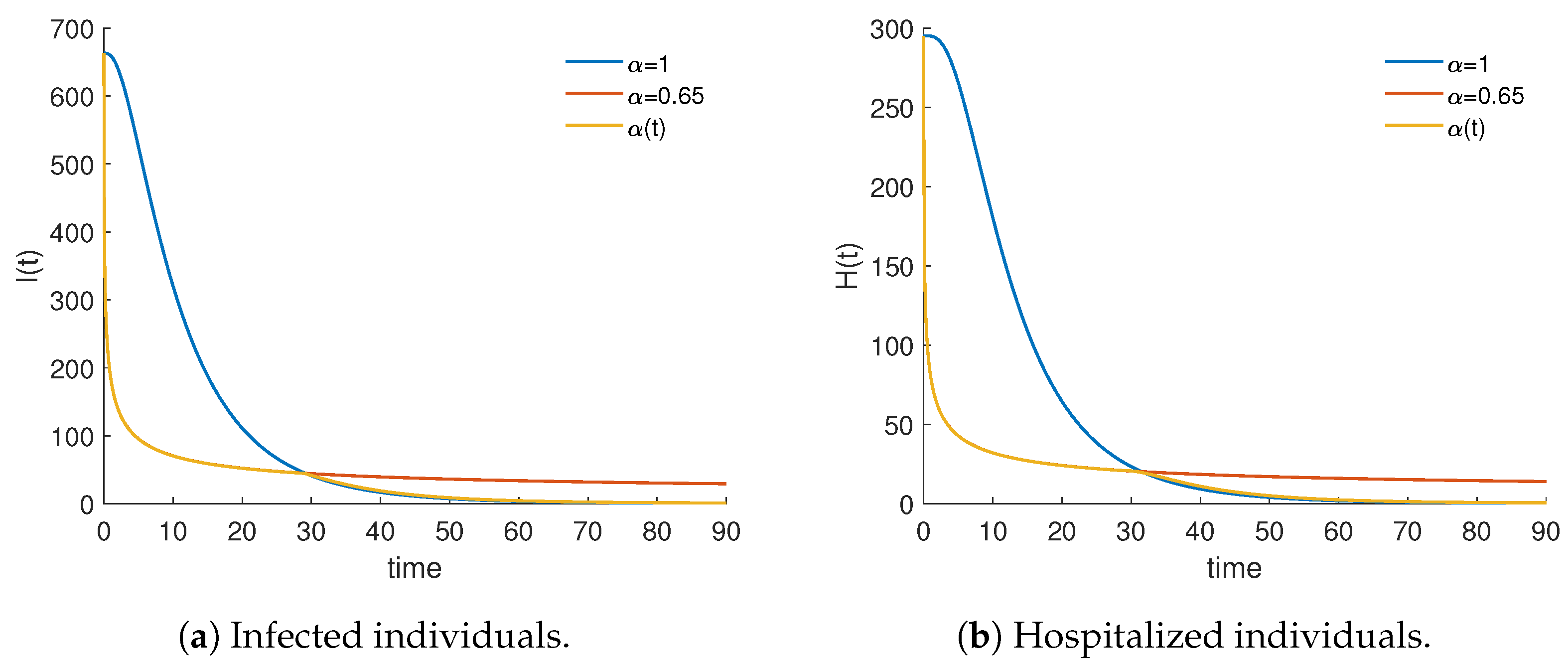
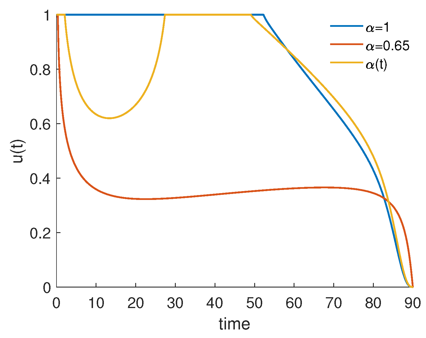
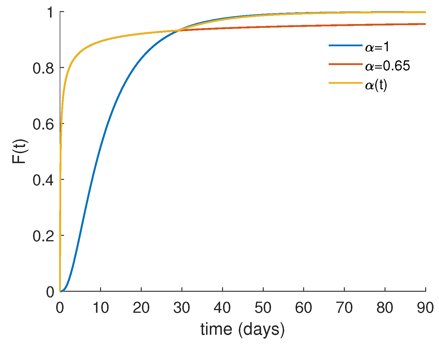
The solutions of the classical and fractional models ($\alpha =1$ and $\alpha =0.65$, respectively) are presented alongside with the solutions of the piecewise derivative system in Figure 6 and Figure 7. The piecewise derivative system’s solutions can be shown to follow the fractional model’s solutions at the beginning and follow the classical model’s solutions at the end of the time interval. This behaviour is seen in Figure 8, which shows the efficacy function for each one of the three studied scenarios.

In

Table 5. Cost-effectiveness measures for the piecewise derivative with fractional Caputo derivatives system with $C=1$.

$\mathbf{AV}$	$\mathbf{TC}$	$\mathbf{ACER}$	$\overline{\mathit{F}}$
56,861.4	48,248.8	0.848534	0.952931

, the cost-effectiveness metrics for the piecewise derivative with fractional Caputo derivatives system are summarized.

The piecewise derivative model is more efficient than the best fractional (cf. Table 5 and Figure 8), being the most effective model, according to our results. This demonstrates the effectiveness of this procedure in controlling the Ebola infection.

5. Conclusions

Ebola infection is still a major health concern in many countries around the world nowadays, particularly in underdeveloped countries where it can have disastrous consequences. In recent years, numerous studies have aimed to control it, as stated in the Introduction.

This work extends and studies a fractional-order mathematical model for Ebola. The estimation of parameters is completed for real data from WHO, minimizing the root mean square deviation. The results show that the proposed model fits the data quite well. Nevertheless, we were unable to identify a derivative order for which the fractional model fits the data better than the classical model. A fractional optimal control problem, having the rate of vaccination as control measure, is then presented, developed and numerically resolved.

The numerical results indicate that the fractional optimal control is more effective and is superior for a portion of the intervention period. As a consequence, we suggest an innovative system in which the derivative order varies over the time interval, becoming an integer or fractional depending on what is better for infection control. This type of variable-order fractional model, known as the piecewise fractional model with Caputo derivatives, proves to be the most successful in managing the dynamics of disease.

As future work, we plan to investigate the usefulness of our fractional approach in other geographical regions and also to extend the presented model to other fractional derivatives.

References

1. World Health Organization. Ebola Virus Disease. Available online: https://www.who.int/news-room/fact-sheets/detail/ebola-virus-disease (accessed on 6 February 2024).
2. Wikipedia. Ebola. Available online: https://en.wikipedia.org/wiki/Ebola (accessed on 16 March 2024).
3. Kaufman, J.S.B.; Jones, A. Ebola Virus Disease. Available online: https://wiki.eclipse.org/Ebola_Models (accessed on 21 March 2024).
4. Area, I.; Ndaïrou, F.; Nieto, J.J.; Silva, C.J.; Torres, D.F.M. Ebola model and optimal control with vaccination constraints. J. Ind. Manag. Optim. 2018, 14, 427–446. [Google Scholar] [CrossRef]
5. Siettos, C.; Anastassopoulou, C.; Russo, L.; Grigoras, C.; Mylonakis, E. Modeling the 2014 ebola virus epidemic–agent-based simulations, temporal analysis and future predictions for liberia and sierra leone. PLoS Curr. 2015, 7. [Google Scholar] [CrossRef]
6. Webb, G.; Browne, C.; Huo, X.; Seydi, O.; Seydi, M.; Magal, P. A model of the 2014 Ebola epidemic in West Africa with contact tracing. PLoS Curr. 2015, 7. [Google Scholar] [CrossRef] [PubMed]
7. Djiomba Njankou, S.D.; Nyabadza, F. Modelling the Role of Human Behaviour in Ebola Virus Disease (EVD) Transmission Dynamics. Comput. Math. Methods Med. 2022, 2022, 4150043. [Google Scholar] [CrossRef] [PubMed]
8. Berge, T.; Lubuma, J.M.S.; Moremedi, G.M.; Morris, N.; Kondera-Shava, R. A simple mathematical model for Ebola in Africa. J. Biol. Dyn. 2017, 11, 42–74. [Google Scholar] [CrossRef] [PubMed]
9. Jiang, S.; Wang, K.; Li, C.; Hong, G.; Zhang, X.; Shan, M.; Li, H.; Wang, J. Mathematical models for devising the optimal Ebola virus disease eradication. J. Transl. Med. 2017, 15, 124. [Google Scholar] [CrossRef] [PubMed]
10. Mhlanga, A. Assessing the impact of optimal health education programs on the control of zoonotic diseases. Comput. Math. Methods Med. 2020, 2020, 6584323. [Google Scholar] [CrossRef] [PubMed]
11. Area, I.; Batarfi, H.; Losada, J.; Nieto, J.J.; Shammakh, W.; Torres, A. On a fractional order Ebola epidemic model. Adv. Differ. Equ. 2015, 2015, 278. [Google Scholar] [CrossRef]
12. Rachah, A.; Torres, D.F.M. Dynamics and optimal control of Ebola transmission. Math. Comput. Sci. 2016, 10, 331–342. [Google Scholar] [CrossRef]
13. Ndaïrou, F.; Khalighi, M.; Lahti, L. Ebola epidemic model with dynamic population and memory. Chaos Solitons Fractals 2023, 170, 113361. [Google Scholar] [CrossRef]
14. Rosa, S.; Torres, D.F.M. Optimal control of a fractional order epidemic model with application to human respiratory syncytial virus infection. Chaos Solitons Fractals 2018, 117, 142–149. [Google Scholar] [CrossRef]
15. Almeida, R. Analysis of a fractional SEIR model with treatment. Appl. Math. Lett. 2018, 84, 56–62. [Google Scholar] [CrossRef]
16. Carvalho, A.R.M.; Pinto, C.M.A. Immune response in HIV epidemics for distinct transmission rates and for saturated CTL response. Math. Model. Nat. Phenom. 2019, 14, 307. [Google Scholar] [CrossRef]
17. Bergounioux, M.; Bourdin, L. Pontryagin maximum principle for general Caputo fractional optimal control problems with Bolza cost and terminal constraints. ESAIM Control Optim. Calc. Var. 2020, 26, 35. [Google Scholar] [CrossRef]
18. Almeida, R.; Pooseh, S.; Torres, D.F.M. Computational Methods in the Fractional Calculus of Variations; Imperial College Press: London, UK, 2015; pp. xii+266. [Google Scholar] [CrossRef]
19. Podlubny, I. Fractional Differential Equations: An Introduction to Fractional Derivatives, Fractional Differential Equations, to Methods of Their Solution and Some of Their Applications; Elsevier: Amsterdam, The Netherlands, 1998. [Google Scholar]
20. Diethelm, K.; Ford, N.J.; Freed, A.D.; Luchko, Y. Algorithms for the fractional calculus: A selection of numerical methods. Comput. Methods Appl. Mech. Eng. 2005, 194, 743–773. [Google Scholar] [CrossRef]
21. Diethelm, K.; Ford, N.J.; Freed, A.D. Detailed error analysis for a fractional Adams method. Numer. Algorithms 2004, 36, 31–52. [Google Scholar] [CrossRef]
22. Diethelm, K.; Ford, N.J.; Freed, A.D. A predictor-corrector approach for the numerical solution of fractional differential equations. Nonlinear Dyn. 2002, 29, 3–22. [Google Scholar] [CrossRef]
23. Lenhart, S.; Workman, J.T. Optimal Control Applied to Biological Models; Chapman & Hall/CRC Mathematical and Computational Biology Series; Chapman & Hall/CRC: Boca Raton, FL, USA, 2007; pp. xii+261. [Google Scholar]
24. Rodrigues, P.; Silva, C.J.; Torres, D.F. Cost-effectiveness analysis of optimal control measures for tuberculosis. Bull. Math. Biol. 2014, 76, 2627–2645. [Google Scholar] [CrossRef] [PubMed]
25. Okosun, K.O.; Rachid, O.; Marcus, N. Optimal control strategies and cost-effectiveness analysis of a malaria model. BioSystems 2013, 111, 83–101. [Google Scholar] [CrossRef] [PubMed]
26. Atangana, A.; İğret Araz, S. New concept in calculus: Piecewise differential and integral operators. Chaos Solitons Fractals 2021, 145, 110638. [Google Scholar] [CrossRef]
27. Rosa, S.; Torres, D.F.M. Fractional-Order Modelling and Optimal Control of Cholera Transmission. Fractal Fract. 2021, 5, 261. [Google Scholar] [CrossRef]
Figure 1. The basic reproduction number, R 0 , of the Ebola model (2) as a function of the fractional derivative order, α .
Mathematics 12 00985 g001
Figure 6. Comparison of state variables I and H of the FOCP (4)–(16), considering classical derivative order ( α = 1 ) and α = 0.65 , with the ones of the piecewise derivative with the fractional Caputo derivatives system.
Mathematics 12 00985 g006
Figure 7. Comparison of control variable u (vaccination) of the FOCP (4)–(16), considering classical derivative order ( α = 1 ) and α = 0.65 , with the one of the piecewise derivative with fractional Caputo derivatives system.
Mathematics 12 00985 g007
Figure 8. Evolution of the efficacy function of the FOCP (4)–(16), considering classical derivative order ( α = 1 ) and α = 0.65 , and of the piecewise derivative with fractional Caputo derivatives system.
Mathematics 12 00985 g008