Article

The Impacts of Payment Schemes and Carbon Emission Policies on Replenishment and Pricing Decisions for Perishable Products in a Supply Chain

Department of Statistics, Tamkang University, Tamsui Dist., New Taipei City 251301, Taiwan
*
Author to whom correspondence should be addressed.
Mathematics 2024, 12(7), 1033; https://doi.org/10.3390/math12071033
Submission received: 6 March 2024 / Revised: 26 March 2024 / Accepted: 27 March 2024 / Published: 29 March 2024
(This article belongs to the Special Issue Innovations in Optimization and Operations Research)

Abstract

:
In the supplier–retailer–consumer system, the retailer’s replenishment and pricing strategies impact the entire transaction process, forming a comprehensive trading market. Suppliers offer advance-cash-credit payments to retailers, while retailers provide customers with cash-credit payment options. In the current health-conscious consumer market, purchasing decisions are influenced not only by commodity prices but also by the freshness of products, particularly perishable goods. Growing awareness of climate change and the advent of carbon emission policies have raised concerns about the environmental costs of business transactions. This study focuses on perishable products whose demand is influenced by both price and freshness. It explores the adoption of various payment methods by suppliers and retailers, as well as the impact of carbon emission cap-and-trade policies or carbon tax policies on management and pricing strategies. Suitable inventory models are established to determine the optimal replenishment and pricing strategies for maximizing the current value of total profit. We illustrate that the current value of total profit demonstrates joint concavity concerning both the selling price and the replenishment time. Finally, we verify the proposed models using numerical examples and present the findings of sensitivity analyses. The findings of this study yield several valuable insights for inventory management of perishable goods.

1. Introduction

The growing frequency of extreme weather events in recent times has significantly increased public awareness about global warming and the environmental effects of greenhouse gases. According to the 2023 edition of the “Global Risks Report” released by the World Economic Forum (WEF), three of the top ten most likely global risks of the future, whether in the short term or long term, are associated with climate change and severe weather patterns. It is widely acknowledged that carbon dioxide emissions are the main driver of global climate change and that the severity of their effects is increasing every year.
To mitigate the impact of these phenomena, multinational organizations and governments across the world have begun to impose stringent restrictions aimed at reducing carbon emissions in virtually all industrial processes. In terms of the “United Nations Framework Convention on Climate Change” of 2015, sometimes referred to as “The Paris Agreement,” countries have reached a consensus on reducing anthropogenic carbon emissions and phasing out greenhouse gas emissions in the latter part of this century. A succession of policies and plans for net-zero greenhouse gas emissions has been proposed following a unique report released by the Intergovernmental Panel on Climate Change (IPCC) in 2018. The top three carbon dioxide emitters in the world, China, the United States (US), and the European Union (EU), have set ambitious carbon reduction targets for 2030: China aims to reduce carbon emissions by more than 65% compared with levels in 2015, the US hopes to reduce emissions by between 50% and 52% compared with levels in 2005, and the EU’s target is to reduce net emissions by 55% compared with 1990. In pursuit of these and analogous goals, numerous countries globally are actively involved in diverse strategic endeavors. These encompass the establishment of novel alternative energy sources, heightened dependence on renewables, enforcement of energy-saving and carbon-reducing regulations, advocacy for carbon trading markets, implementation of carbon tax collection systems, and incorporation of carbon offset mechanisms.
Implementation of these policies and measures is undoubtedly affecting the operations of most businesses. As the external costs associated with emissions can be debilitating, businesses that neglect imperatives to curb emissions when making operational decisions can potentially jeopardize their survival and growth. Furthermore, reducing carbon emissions not only contributes to cost savings but also enhances operational efficiency. As a result, the influence of carbon emissions on operational management has recently begun to garner increased academic attention, with the reduction of carbon emissions emerging as a particular concern in inventory management. Consequently, there is now a substantial body of literature examining production and inventory models in the context of carbon emission reduction policies (see, for example, An et al. [1], Dong et al. [2], Fu et al. [3], Hammami et al. [4], Lu et al. [5], Ma et al. [6], Maulana et al. [7], Mishra et al. [8], Mubin et al. [9], Sabzevar et al. [10], Sarkar et al. [11], Shi et al. [12]). Dye and Yang [13], for instance, introduced an inventory system for perishable goods that incorporates a range of different carbon emission policies and accounts for the influence of trade credit risk. Their aim was to determine the best credit period and inventory replenishment strategies to maximize the total profit per unit of time for the retailer. Daryanto et al.’s [14] study of a three-echelon supply chain model takes into account both carbon emissions and deteriorating items. Ma et al. [15] addressed the issue of spoiled goods encountered by suppliers and retailers, considering market demand influenced by factors such as selling price, freshness, and environmental sustainability within the limitations of cap-and-trade regulations. Cheng et al. [16] formulated an extensive inventory model that incorporates pricing, pre-sale incentives, advance sales, trade credit, and carbon tax policies. With the aim of achieving sustainable development objectives, the proposed model also integrates considerations for carbon tax policies. The objective is to determine optimal pricing, pre-order discounts, and replenishment decisions under carbon tax policies, thereby maximizing total profit. Jain et al. [17] proposed a three-echelon supply chain inventory model incorporating several regulatory strategies, including carbon offset, carbon tax, and carbon cap-and-trade regulations. The objective of their study was to identify how to minimize total cost while simultaneously reducing carbon emissions.
Despite the growing body of literature on the impacts of carbon reduction policies on trade and industry, payment options are an aspect of inventory and operations management and a topic worthy of exploration. In today’s highly competitive markets, sellers typically encounter three types of payment options: (1) advance payment, also known as cash in advance, where the buyer pays the seller for goods and services before the delivery takes place; (2) cash payment, or cash on delivery, where the buyer settles the payment immediately upon receiving the goods or services; and (3) credit payment, which allows the buyer to delay payment within certain permissible terms, with the seller offering goods or services as soon as the buyer receives them. In the traditional inventory model, the assumed payment method is cash payment, which is inconsistent with the current business transaction method. In actual business transactions, it is common for suppliers to request that buyers make either full or partial payment of the purchase cost within a specified timeframe prior to the scheduled delivery date. This practice is aimed at minimizing the risks associated with payment defaults. Advance payment schemes are, therefore, widely adopted and valuable in reducing estimation errors in demand. Furthermore, suppliers often provide retailers with attractive credit terms as a means of boosting sales and minimizing inventory levels. Trade credit, in particular, can be viewed as an alternative to pricing discounts as it avoids triggering pricing wars with competitors, which in turn could lead to sustained price reductions. As a result, trade credit has gained popularity and is now a significant strategic consideration in company financial planning and management.
Extensive research has been conducted on the interplay between inventory policies and trade credit. Following Goyal’s [18] pioneering formulation of the initial economic order quantity (EOQ) model for a constant demand rate, which takes into account permissible delays in payments, numerous articles have explored similar or related issues, often considering more generalized assumptions. For example, Teng [19] expanded upon Goyal’s [18] model by integrating the difference between purchase cost and selling price. This research uncovered that, in specific situations, the economic replenishment interval and order quantity decrease with the introduction of a permissible payment delay. Chang et al. [20] suggested an EOQ model specifically tailored for perishable products, while Teng [21] explored scenarios where suppliers provide full trade credit to reliable customers and partial trade credit to less dependable customers. Teng et al. [22] later developed an optimal ordering policy for stock-dependent demand in the context of a progressive payment scheme. This analysis was subsequently expanded by considering shifts from constant demand to patterns of non-decreasing demand (Teng et al. [23]). Ouyang and Chang [24] explored an economic production quantity (EPQ) model that integrates imperfect production processes, permissible payment delays, and complete backlogging. Sarkar et al. [25] formulated an integrated inventory model accounting for lead time, defective units, and payment delays. Similarly, Liao et al. [26] obtained an optimal strategy for managing perishable items with capacity constraints by incorporating a two-level trade credit system. Chang et al. [27] developed an inventory model for retailers, examining the impact of defective items and trade credits on replenishment decisions. Majumder et al. [28] introduced an EPQ model specifically tailored for deteriorating substitute items, taking into account the implementation of a trade credit policy. Panda et al. [29] introduced a method for credit policy in a two-warehouse inventory model centered on deteriorating items, demand dependent on price and stock, and partial backlogging.
Considerable academic research has been conducted on the specific topic of advance payment. Following Zhang’s [30] advance payment scheme that incorporates a fixed per-payment cost to enhance time and cost savings, Maiti et al. [31] proposed an inventory model that incorporates stochastic lead time and advance payment, as well as a modified version that also considers price-dependent demand. A novel approach to addressing the joint-replenishment inventory control problem for multiple products was presented by Taleizadeh et al. [32], whose model considers partial payment in advance for raw materials imported from another country. Thangam [33] examined strategies for optimal price discounting and lot-sizing policies specifically tailored for deteriorating items within a supply chain, focusing particularly on the implementation of an advance payment scheme with two-echelon trade credits. Taleizadeh et al. [34] proposed an EOQ model that allows for limited backordering in scenarios where buyers are required to make partial prepayments in multiple installments. Taleizadeh [35] later offered two distinct EOQ models for managing deteriorating items in the context of multiple prepayments, one that considers shortages and another that does not. In these two models, the prepayments are structured as consecutive equal-sized payments. With the aim of analyzing the effects of advance payment on a firm’s inventory policy, Zhang et al. [36] developed an inventory model that incorporates various types of advance payment terms.
Several noteworthy studies have considered the implications of lot sizing in inventory management. For example, Teng et al. [37] examined lot-size policies for managing perishable items with expiration dates, and Taleizadeh et al. [38] considered a lot sizing model that incorporates advance payment and planned backordering. Feng et al. [39] investigated an inventory system that incorporates several factors, including a demand curve influenced by unit price, displayed volume, and sell-by date. This study also considered the adoption of an advance-cash-credit (ACC) payment scheme by the supplier and the retailer. The primary objective for the retailer is to maximize total profit by determining the optimal price and order cycle simultaneously. Recently, Tsao et al. [40] established a single supplier–manufacturer chain where the manufacturer received an ACC payment from a supplier. The model incorporates imperfect EPQ for deteriorating products, with predictive maintenance applied by the manufacturer. This study aims to identify the optimal replenishment cycle time and predictive maintenance effort to minimize the present value of the total cost. Several other noteworthy and pertinent studies on advance payment have been conducted, including those by Li et al. [41], Wu et al. [42], Chang et al. [43], Shi et al. [12], Taleizadeh et al. [44], and Shi et al. [45].
It is widely recognized in traditional marketing and economic theory that an inverse relationship exists between price and demand, with the result that higher prices tend to produce lower demand. Selling price, therefore, plays a pivotal role in influencing consumer demand and has a significant impact on purchasers’ decision-making processes. Against a backdrop of increasingly health-conscious consumer preferences, there is a clear inclination towards purchasing perishable goods that are fresh and far from their sell-by expiration dates. In view of this, the aging of perishable goods detrimentally impacts demand as it leads to a loss of product freshness. Several works have addressed inventory management of fresh produce. Wu et al. [46] investigated inventory management in situations where time-varying demand is influenced by stock level, product freshness, and expiration date. Chen et al. [47] expanded on this by considering shelf space as another decisive variable. Li and Teng [48] examined pricing and lot-sizing strategies in scenarios where demand is influenced by reference price, selling price, product freshness, and displayed stocks, while Shi et al. [12] formulated a supply chain model suitable for situations where the demand for perishable goods is contingent on both stock age and selling price. Other notable studies which consider the relationship between product freshness and expiration date include the works of Wang et al. [49], Wu et al. [42], Taleizadeh et al. [50], and Shi et al. [45]. With this literature in mind, it is reasonable to assume that the demand for perishable goods can be modeled as a function of both unit price and stock age.
It is evident from the preceding discussion that trade credit plays a significant role in shaping inventory policies, affecting both the costs for suppliers and the benefits for buyers. Credit is clearly an integral and unavoidable component of contemporary trade transactions, and its influence cannot be overlooked. Advance payment schemes are widely prevalent and highly favored as a payment method, particularly for mitigating the risk of default. Considering the joint impact of selling price and stock age on the demand for perishable products, the influence of carbon emission reduction policies on pricing, credit terms, and operational management practices has become increasingly crucial in today’s landscape. To address the practical challenges of inventory management and real-world market dynamics, this paper examines the impacts of the ACC payment scheme and carbon emission policies on the pricing and replenishment decisions of retailers who deal with perishable goods. Given that the primary distinction between different payment types lies in the timing of payments, which in turn affects the time value of money associated with purchasing costs, discounted cash-flow analysis is a suitable approach for evaluating the impact of these payment types. This paper thus develops EOQ models for perishable products that account for the influence of both ACC payment schemes and carbon emission policies. Given that the demand for perishable goods depends on both unit price and stock age, these models will be crafted utilizing a discounted cash-flow analysis methodology. The primary aim is to determine the optimal selling price, order quantity, and replenishment time for a retailer to maximize the current value of total annual profit. A summary comparison of the relevant models is presented in Table 1.
The subsequent parts of this paper are segmented into seven sections. Section 2 presents the notations and assumptions utilized in this study, while Section 3 formulates various mathematical models. Theoretical findings are presented in Section 4, followed by the illustration of the proposed models through numerical examples in Section 5. In Section 6, a sensitivity analysis is conducted, and practical insights for management processes are provided. Section 7 outlines the study’s conclusions.

2. Notations and Assumptions

This article will employ the subsequent notations and assumptions.
Notations:
f 1 the portion of the procurement cost that must be paid upfront, 0 f 1 1
f 2 the portion of the procurement cost payable upon delivery, 0 f 2 1
f 3 the portion of the procurement cost that allows for an acceptable delay from the supplier to the retailer, 0 f 3 1 and f 1 + f 2 + f 3 = 1
k l the duration of credit extended by the retailer to customers, i.e., the downstream credit period, k l 0
k u the duration of credit offered by the supplier to the retailer, i.e., the upstream credit period, k u 0
ρ the proportion of sales revenue that allows for an acceptable delay from the retailer to customers, 0 ρ 1
γ the annual compound interest paid per dollar
t 0 the duration over years for which prepayments are made, t 0 > 0
c the procurement cost per unit in dollars, c > 0
h the holding cost per unit per year in dollars, excluding interest charges, h > 0
b carbon emissions generated during the purchase of a single unit of the product
h e carbon emissions resulting from inventory holding per unit over a given timeframe
o e carbon emissions generated by an order
c e unit carbon trading emission price or unit carbon tax
B carbon emission cap for the retailer
I p the annual interest charged by the supplier per dollar
I e the annual interest earned per dollar
x the duration until the expiration date or shelf life, i.e., the stock age, measured in years, x > 0
o the cost of ordering, expressed in dollars per order, o > 0
S the selling price per unit in dollars, S > c > 0 (decision variable)
t the time in years, t 0
D t ,   S the annual demand rate, D t ,   S = f S x t / x   ,   f S > 0 ,   f S < 0 and f ( S ) > 0
θ t the deteriorating rate at time t ,   0 θ t 1 ,   θ t 0 and θ x = 1
I t the inventory level in units at time t
Q the order quantity
T the duration of the cycle period, measured in years, T x (decision variable)
P T P the current value of the overall annual profit in dollars
I C 1 the current value of interest incurred for advance payment per cycle period T
I C 2 the current value of interest incurred for cash payment per cycle period T
I C 3 the current value of interest incurred for credit payment per cycle period T
I E 1 the current value of interest accrued for credit payment per cycle period T
C C the current value of capital cost per cycle period T
Assumptions:
(1)
Shortages are prohibited.
(2)
The ending inventory is zero.
(3)
The freshness and demand of perishable products are absolutely related to the stock age; hence, the demand rate is assumed as a function of selling price S and stock age x , that is, D t ,   S = f S x t / x   ,   0 t x , where f S > 0 ,   f S < 0 and f S > 0 .
(4)
During the credit period k u provided by the upstream supplier, the unsettled account allows for the generated sales revenue to be deposited into an interest-bearing account. Once the permissible delay period elapses, the retailer settles the remaining procurement cost and proceeds to pay the accrued interest charges on the items in stock. The downstream credit period, k l , is offered by the retailer. Consequently, the retailer can amass revenue in an account and acquire earned interest when k u k l . There is no interest earned for the retailer when k u < k l . Because the product cannot be sold after the expiration date, it is assumed that k l x and k u x .
(5)
The supplier asks that the retailer (i) prepay f 1 percentage of procurement cost in t 0 years prior to the time of delivery, (ii) pay another f 2 percentage of procurement cost at the time of delivery, and (iii) offer a credit period of k u years on the remaining f 3 percentage of procurement cost (i.e., 0 f 1 , f 2 , f 3 1 , and f 1 + f 2 + f 3 = 1 ). Similarly, the retailer extends partial trade credit to customers, allowing them a credit period of k l years for ρ proportion of sales, while the remaining portion (i.e., 1 ρ proportion of sales) is paid in cash.
(6)
Two main policy approaches apply to carbon emission reduction: the carbon cap-and-trade policy and the carbon tax policy. Within the framework of the carbon cap-and-trade policy, the retailer is assigned an initial cap for carbon emissions and has the flexibility to trade or exchange emission rights within this established cap. If the retailer exceeds its carbon cap B , it must purchase extra carbon allowances from the compliance carbon trading market to offset the difference between its actual emissions and the established cap. In the scenario where the retailer’s carbon emissions fall below its carbon cap, however, the retailer will have the opportunity to trade its surplus carbon allowances with other businesses on the compliance carbon trading market. In the carbon tax policy, the focus is solely on the amount of tax imposed on total carbon emissions, without considering other factors or mechanisms such as trading or allowances. The carbon emissions of the retailer primarily originate from various operational activities, encompassing tasks such as ordering, purchasing, and storage.
The purpose of this paper is to determine the optimal selling price, order quantity, and replenishment time for a retailer to maximize the current value of total annual profit when an ACC payment scheme is adopted by the supplier, the retailer offers customers a cash-credit (CC) payment method, and the carbon emissions cap-and-trade or carbon tax is considered. We, therefore, assume that the supplier agrees to an ACC payment scheme, the retailer likewise offers customers a CC payment method, and either the carbon emissions cap or carbon tax policy is included. The demand rate is considered to be dependent on both the selling price and the age of the stock (i.e., D t ,   S ). The discounted cash-flow approach is adopted to discuss the current value of total annual profit for a retailer.

3. Mathematical Model Formulation

According to the above notations and assumptions, the inventory level at time t is given by the following differential equation:
d I ( t ) d t = D ( t , S ) θ ( t ) I ( t ) = x t x f ( S ) θ ( t ) I ( t ) , 0 t T x
with boundary condition I ( T ) = 0 . Solving Equation (1) with boundary condition I ( T ) = 0 , we obtain
I ( t ) = e 0 t θ ( u ) d u t T x v x f ( S ) e 0 v θ ( u ) d u d v , 0 t T x
Using (2), the order quantity delivered at time 0 is obtained as follows:
Q = I ( 0 ) = 0 T x v x f ( S ) e 0 v θ ( u ) d u d v = 0 T D ( v , S ) e 0 v θ ( u ) d u d v
Hence, excluding the consideration of the time value of money, the total procurement cost is given by
c Q = c I ( 0 ) = c f ( S ) 0 T x v x e 0 v θ ( u ) d u d v
Since the ACC payment scheme is adopted by the supplier, the total procurement cost is subdivided into three payments as delineated below: (1) the advance payment at t 0 years before time 0 , (2) the cash payment at time 0 , and (3) the credit payment at time k u . Therefore, the current value of total procurement cost per cycle time T is given as
P C = f 1 c Q e γ t 0 + f 2 c Q + f 3 c Q e γ k u = f 1 e γ t 0 + f 2 + f 3 e γ k u c f S 0 T x v x e 0 v θ u d u d v
As the retailer’s ordering occurs t 0 years before the delivery time 0 , the current value of order cost at time t 0 is described as
O C = o e γ t 0
The current value of the holding cost, excluding the interest charged, per cycle time T is shown as follows:
H C = h 0 T I t e γ t d t = h 0 T e 0 t θ u d u t T D v , S e 0 v θ u d u d v e γ t d t = h f S 0 T t T x v x e t v θ u d u γ t d v d t
The retailer offers customers a partial downstream credit period k l on ρ proportion of sales. The customer receives items at time t and is required to pay 1 ρ proportion of sales in cash, while the ρ proportion of sales is paid at time t + k l . Hence, the retailer’s current value of sales revenue per cycle time T is as follows:
S R = ρ S f S k l T + k l x t + k l x e γ t d t + ( 1 ρ ) S f ( S ) 0 T x t x e γ t d t
When the carbon cap-and-trade policy is applied, the retailer’s amount of carbon emissions includes carbon emissions from the buying, holding, and ordering process. In addition, the retailer’s carbon emission cap is B . Therefore, the carbon emissions cost is equal to the unit carbon trading price c e multiplied by the difference between the retailer’s amount of carbon emissions and the carbon emission cap. So, the quantity of carbon emissions and the current value of carbon emissions cost per cycle time T can be calculated, respectively, as follows:
A E = o e + b Q + h e 0 T I ( t ) d t
and
C E = c e o e e γ t 0 + b Q + h e 0 T I ( t ) e γ t d t B T
Note: In Equation (10), if B = 0 , then C E is the current value of the carbon emissions tax per cycle time T and the carbon tax policy is adopted.
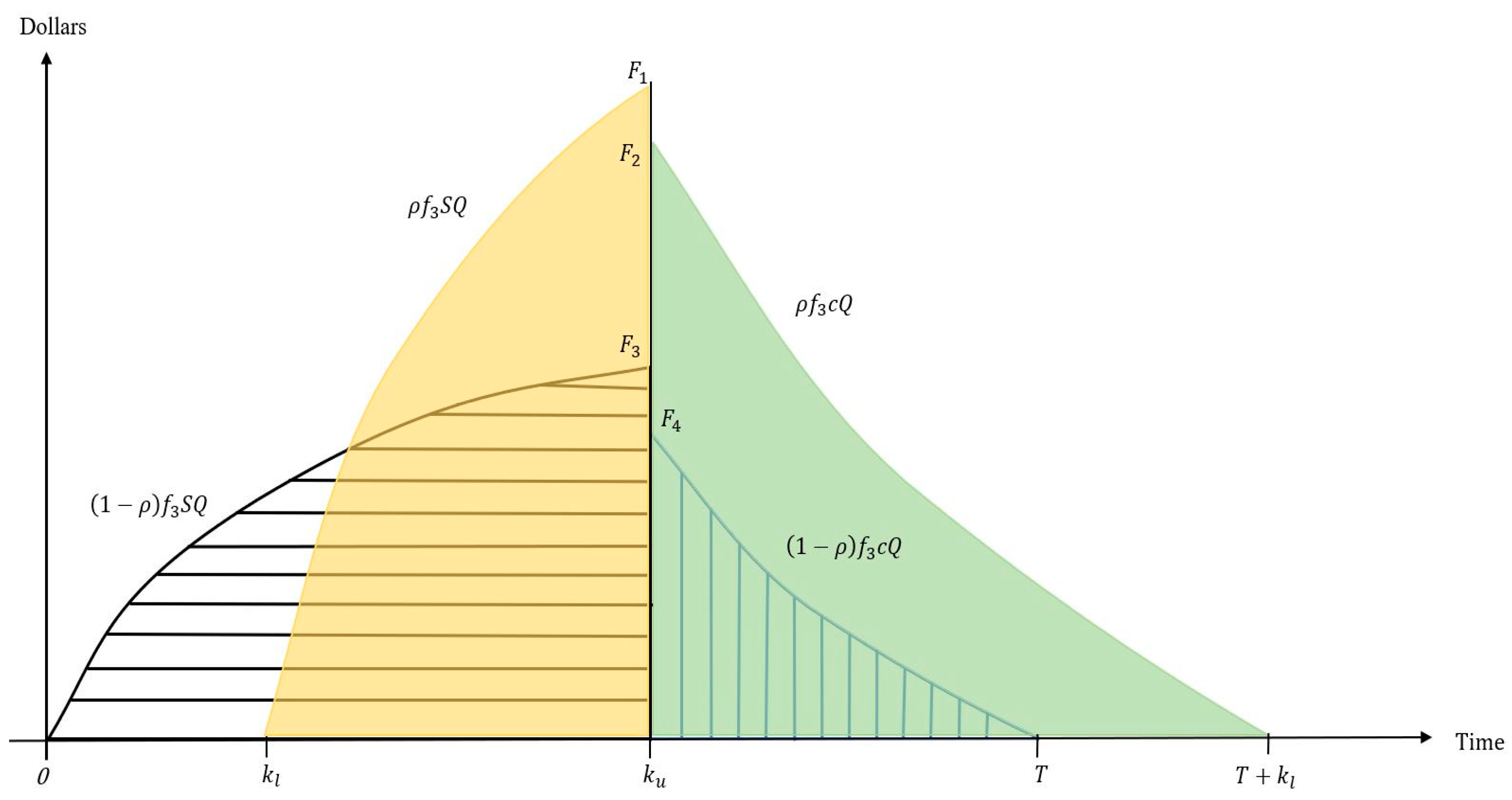
The current value of capital cost consists of (i) the interest charged for advance payment, (ii) the interest charged for cash payment, and (iii) the interest charged or earned for credit payment. Figure 1 shows the current values of interest charged for advance payment and cash payment.
For the advance payment, the interest charged is shown in both areas t 0 ,   F 1 , F 2 , k l and ( k l , F 2 , T + k l ) of Figure 1. So,
I C 1 = I p c f S f 1 t 0 k l e γ t d t 0 T x t x e 0 t θ u d u d t + f 1 c I p f S k l T + k l e γ t t T + k l x v x d v d t
For the cash payment, the interest charged is shown in both areas ( 0 ,   F 3 , F 4 , k l ) and ( k l , F 4 ,   T + k l ) of Figure 1. Hence,
I C 2 = I p c f S f 2 0 k l e γ t d t 0 T x t x e 0 t θ u d u d t + f 2 c I p f ( S ) k l T + k l e γ t t T + k l x v x d v d t
For the credit payment, according to the values of upstream credit period k u and downstream credit period k l , there are two potential cases for interest charged or earned: (i) k l k u and (ii) k l k u . Each is discussed separately below.
Case 1:  k l k u
With the retailer offering partial trade credit to customers, T + k l represents the point in time when the retailer receives the final payment from the customer for ρ proportion of sales. Based on the values of k u , T, and T + k l , there exist three potential sub-cases.
Case 1.1:  k l k u  and  k u T T + k l
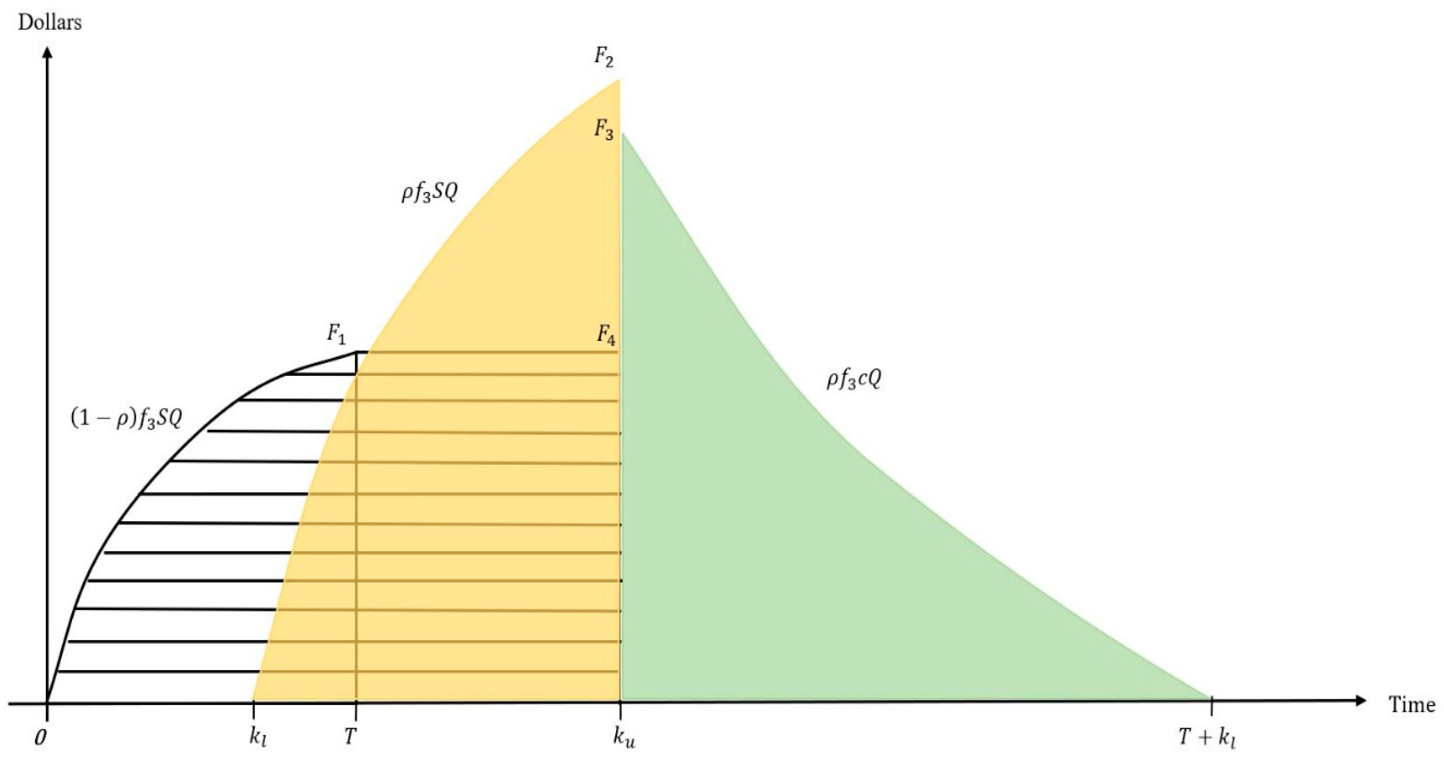
The interest charged is shown in both areas ( k u , F 2 ,   T + k l ) and ( k u ,   F 4 ,   T ) of Figure 2. Thus,
I C 3 = f 3 c I p f ( S ) ρ k u T + k l e γ t t T + k l x v x d v d t + ( 1 ρ ) k u T e γ t t T x v x d v d t
The interest earned is presented in both areas ( k l , F 1 , k u ) and ( 0 ,   F 3 , k u ) of Figure 2. Hence,
I E 3 = f 3 S I e f ( S ) ρ k l k u e γ t k l t x v x d v d t + ( 1 ρ ) 0 k u e γ t 0 t x v x d v d t
From (11)–(14), the current value of capital cost per cycle time T is obtained as
C C 1 = I C 1 + I C 2 + I C 3 I E 3
Using (4)–(8), (10) and (15), the current value of total annual profit is obtained by
P T P 1 S , T = 1 T S R O C P C H C C C 1 C E = 1 T ρ S f S k l T + k l x t + k l x e γ t d t + 1 ρ S f S 0 T x t x e γ t d t e γ t 0 o + c e o e f 1 e γ t 0 + f 2 + f 3 e γ k u c + c e b f S 0 T x v x e 0 v θ u d u d v h + c e h e f S 0 T t T x v x e t v θ u d u γ t d v d t I p c f S f 1 t 0 k l e γ t d t + f 2 0 k l e γ t d t 0 T x t x e 0 t θ u d u d t f 1 + f 2 c I p f S k l T + k l e γ t t T + k l x v x d v d t f 3 c I p f S ρ k u T + k l e γ t t T + k l x v x d v d t + 1 ρ k u T e γ t t T x v x d v d t + f 3 S I e f S ρ k l k u e γ t k l t x v x d v d t + 1 ρ 0 k u e γ t 0 t x v x d v d t + c e B T }
Case 1.2:  k l k u  and  T k u T + k l
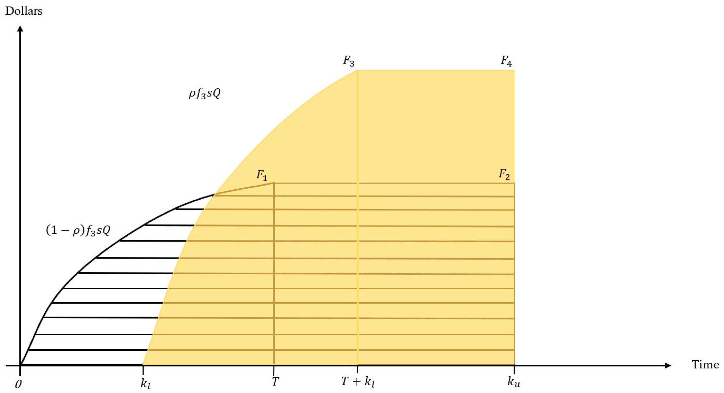
In Figure 3, the cumulative sales volume per cycle time T is shown as
0 T D ( t , S ) d t = 0 T x t x f ( S ) d t = f ( S ) T T 2 2 x
The interest charged is shown in the area ( k u , F 3 , T + k l ) of Figure 3. Hence,
I C 3 = f 3 c I p f ( S ) ρ k u T + k l e γ t t T + k l x v x d v d t
Using (17) as well as both areas ( k l , , F 2 , k u ) and ( 0 , F 1 , F 4 , k u ) of Figure 3, we obtain
I E 3 = ρ f 3 S I e f S k l k u e γ t k l t x v x d v d t + 1 ρ f 3 S I e f S 0 T e γ t t T x v x d v d t + T T 2 2 x T k u e γ t d t
From (11), (12), (18) and (19), the current value of capital cost per cycle time T is yielded as
C C 2 = I C 1 + I C 2 + I C 3 I E 3
Using (4)–(8), (10) and (20), the current value of total annual profit is obtained by
P T P 2 S , T = 1 T S R O C P C H C C C 2 C E = 1 T ρ S f S k l T + k l x t + k l x e γ t d t + 1 ρ S f S 0 T x t x e γ t d t e γ t 0 o + c e o e f 1 e γ t 0 + f 2 + f 3 e γ k u c + c e b f S 0 T x v x e 0 v θ u d u d v h + c e h e f S 0 T t T x v x e t v θ u d u γ t d v d t I p c f S f 1 t 0 k l e γ t d t + f 2 0 k l e γ t d t 0 T x t x e 0 t θ u d u d t f 1 + f 2 c I p f S k l T + k l e γ t t T + k l x v x d v d t f 3 c I p f S ρ k u T + k l e γ t t T + k l x v x d v d t + f 3 S I e f S ρ k l k u e γ t k l t x v x d v d t + 1 ρ f 3 S I e f S 0 T e γ t t T x v x d v d t + T T 2 2 x T k u e γ t d t + c e B T }
Case 1.3:  k l k u  and  k u T + k l
All revenue is received by the retailer at time T + k l , and the supplier is paid the f 3 percentage of the procurement cost at time k u , as outlined in Figure 4.
Therefore, the interest charge is not incurred for credit payment. The interest earned is shown in both areas ( k l , , F 3 , F 4 , k u ) and ( 0 , F 1 , F 2 , k u ) of Figure 4. Thus,
I E 3 = ρ f 3 S I e f S k l T + k l e γ t t T + k l x v x d v d t + T T 2 2 x T + k l k u e γ t d t + ( 1 ρ ) f 3 S I e f ( S ) 0 T e γ t t T x v x d v d t + T T 2 2 x T k u e γ t d t
From Equations (11), (12) and (22), the current value of capital cost per cycle time T is shown as
C C 3 = I C 1 + I C 2 I E 3
Combining (4)–(8), (10) and (23), the current value of total annual profit is obtained as
P T P 3 S , T = 1 T S R O C P C H C C C 3 C E = 1 T ρ S f S k l T + k l x t + k l x e γ t d t + 1 ρ S f S 0 T x t x e γ t d t e γ t 0 o + c e o e f 1 e γ t 0 + f 2 + f 3 e γ k u c + c e b f S 0 T x v x e 0 v θ u d u d v h + c e h e f S 0 T t T x v x e t v θ u d u γ t d v d t I p c f S f 1 t 0 k l e γ t d t + f 2 0 k l e γ t d t 0 T x t x e 0 t θ u d u d t f 1 + f 2 c I p f S k l T + k l e γ t t T + k l x v x d v d t + ρ f 3 S I e f S k l T + k l e γ t t T + k l x v x d v d t + T T 2 2 x T + k l k u e γ t d t + 1 ρ f 3 S I e f S 0 T e γ t t T x v x d v d t + T T 2 2 x T k u e γ t d t + c e B T }
Case 2:  k l k u
The interest earned for credit payment is not incurred, as indicated in Figure 5. The interest charged is shown in both areas k u ,   F 2 ,   F 3 ,   T + k l and ( k u , F 1 , T ) of Figure 5. Thus,
I C 3 = f 3 c I p f S ρ T T 2 2 x k u k l e γ t d t + k l T + k l e γ t t T + k l x v x d v d t + ( 1 ρ ) k u T e γ t t T x v x d v d t
The interest earned is shown as the area ( 0 , F 1 , k u ) in Figure 5. Hence,
I E 3 = f 3 S I e f ( S ) ( 1 ρ ) 0 k u e γ t 0 t x v x d v d t
From (11), (12), (25) and (26), the current value of capital cost per cycle time T is obtained as
C C 4 = I C 1 + I C 2 + I C 3 I E 3
Hence, using (4)–(8), (10) and (27), the current value of total annual profit is as follows:
P T P 4 S , T = 1 T S R O C P C H C C C 4 C E = 1 T ρ S f S k l T + k l x t + k l x e γ t d t + 1 ρ S f S 0 T x t x e γ t d t e γ t 0 o + c e o e f 1 e γ t 0 + f 2 + f 3 e γ k u c + c e b f S 0 T x v x e 0 v θ u d u d v h + c e h e f S 0 T t T x v x e t v θ u d u γ t d v d t I p c f S f 1 t 0 k l e γ t d t + f 2 0 k l e γ t d t 0 T x t x e 0 t θ u d u d t f 1 + f 2 c I p f S k l T + k l e γ t t T + k l x v x d v d t f 3 c I p f S ρ T T 2 2 x k u k l e γ t d t + k l T + k l e γ t t T + k l x v x d v d t + 1 ρ k u T e γ t t T x v x d v d t + f 3 S I e f S 1 ρ 0 k u e γ t 0 t x v x d v d t + c e B T }

4. Theoretical Findings

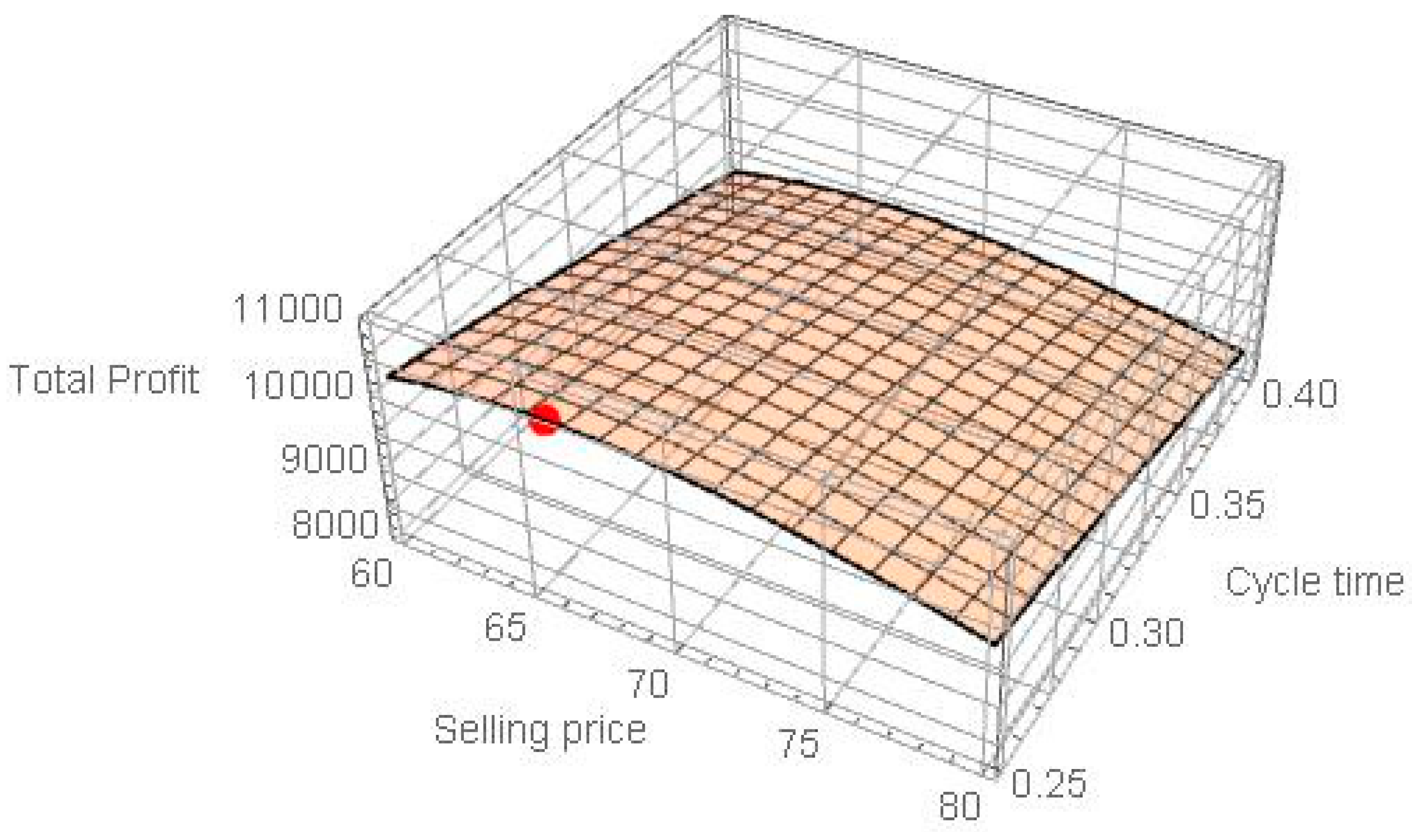
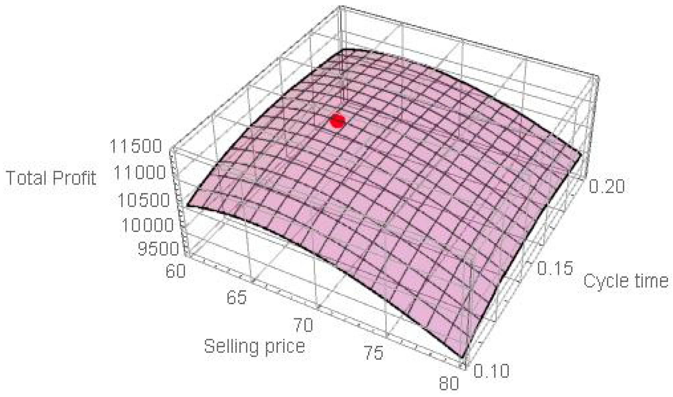
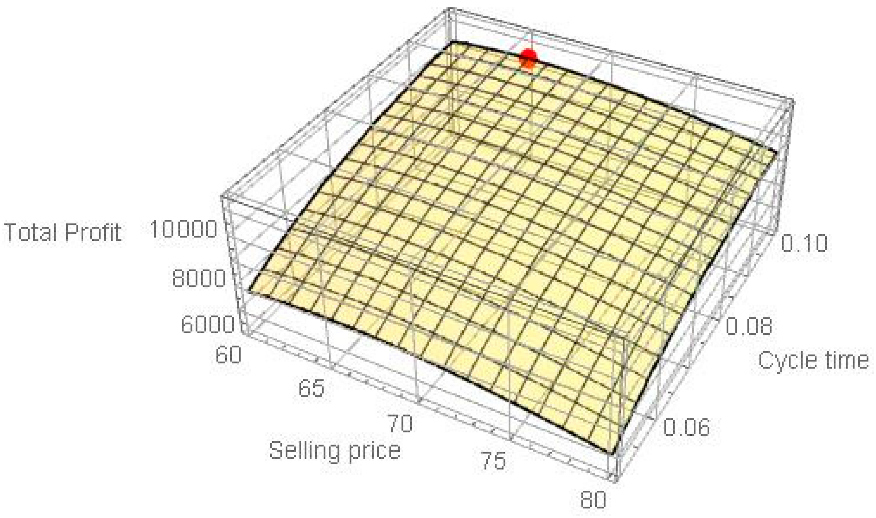
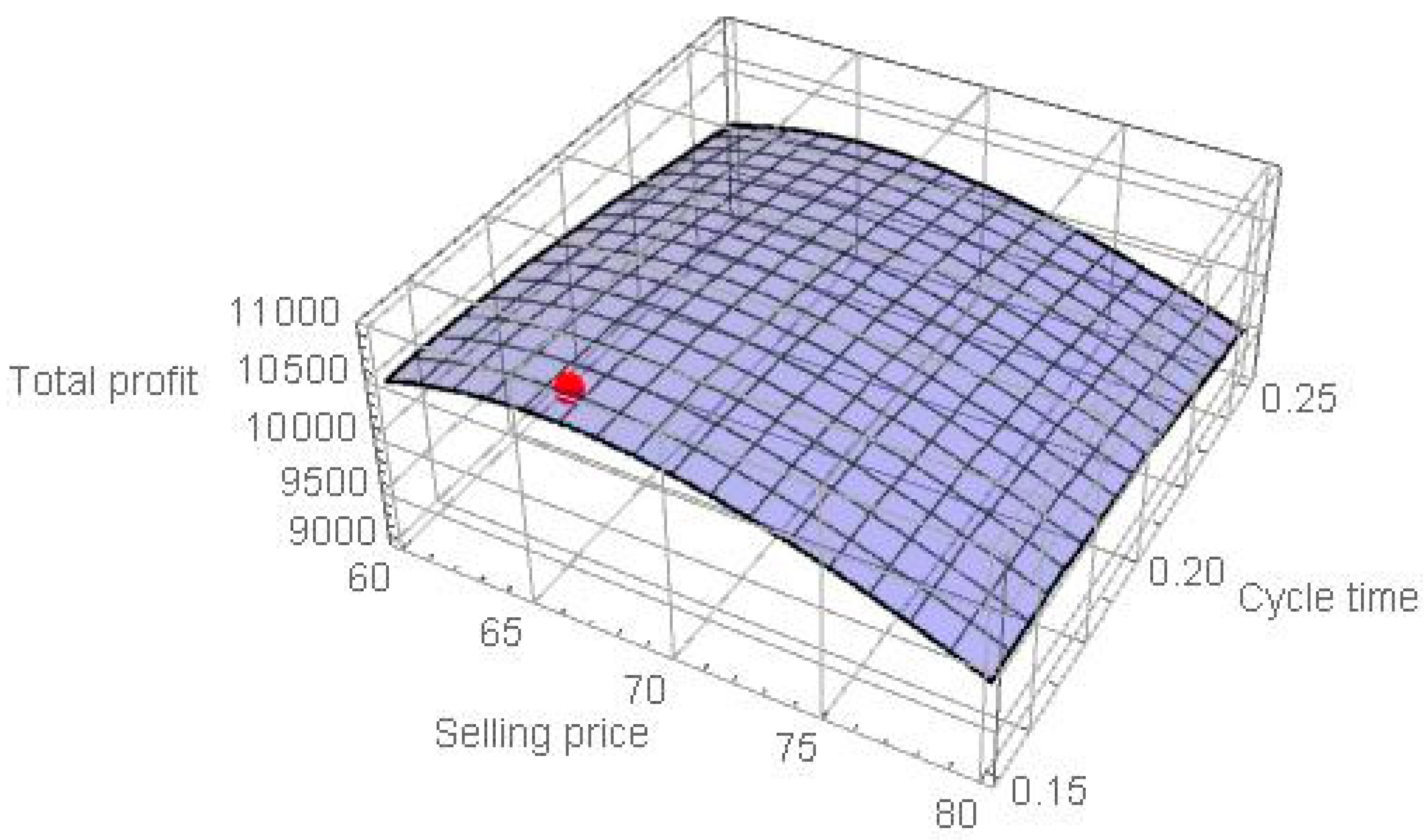
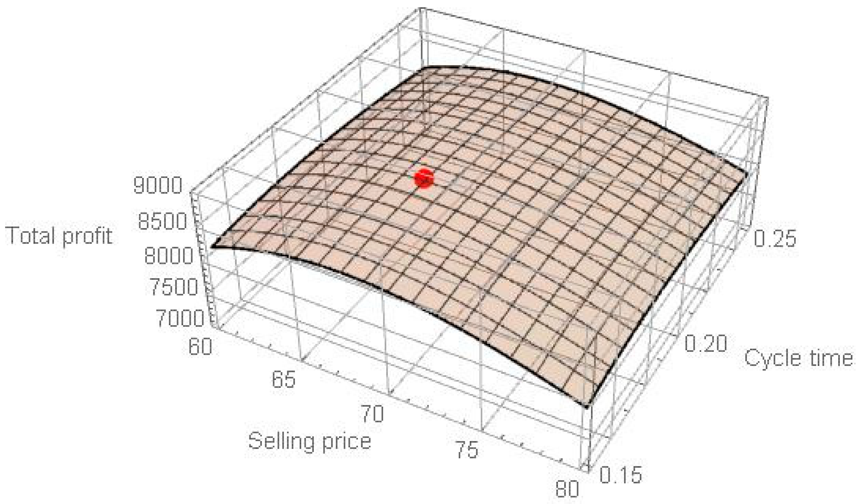
We now discuss the cases of k l k u and k l k u . Because of the intricacy of the problem, demonstrating the joint concavity of the current value of total annual profit over S and T does not appear straightforward. We use the first-order derivative of P T P i ( S , T ) , i = 1, 2, 3, and 4 to determine the optimal solution. We then check the sufficient condition that the Hessian is negative-definite by applying the software Mathematica 13.1 to numerical examples. In addition, the graphs of P T P i ( S , T ) , i = 1, 2, 3, and 4, as shown in Figure 6, Figure 7, Figure 8, Figure 9, Figure 10 and Figure 11 below, indicate that P T P i ( S , T ) , i = 1, 2, 3, and 4 are jointly concave over both S and T .

4.1. Case 1: k l k u

Case 1.1:  k l k u  and  k u T T + k l
In order to optimize the current value of total annual profit, we take the first-order derivative of P T P 1 ( S , T ) in (16) with respect to T and S , respectively, set the results to zero, and re-arrange terms. The optimal replenishment time T 1 and selling price S 1 are then determined as follows:
ρ S f S x T T 2 x e γ T + k l k l T + k l x t + k l x e γ t d t + 1 ρ S f S x T T 2 x e γ T 0 T x t x e γ t d t + o + c e o e e γ t 0 f 1 e γ t 0 + f 2 + f 3 e γ k u c + c e b f S x T T 2 x e 0 T θ u d u 0 T x t x e 0 t θ u d u d t h + c e h e f S T 0 T x T x e t T θ u d u γ t d t 0 T t T x v x e t v θ u d u γ t d v d t c I p f S f 1 t 0 k l e γ t d t + f 2 0 k l e γ t d t x T T 2 x e 0 T θ u d u 0 T x t x e 0 t θ u d u d t f 1 + f 2 c I p f S T k l T + k l e γ t x T k l x d t k l T + k l e γ t t T + k l x v x d v d t f 3 c I p f S ρ k u T + k l e γ t T x T k l x t T + k l x v x d v d t + 1 ρ k u T e γ t x T T 2 x t T x v x d v d t f 3 S I e f S ρ k l k u e γ t k l t x v x d v d t + 1 ρ 0 k u e γ t 0 t x v x d v d t = 0
and
f ( S ) + S f ( S ) U 1 f ( S ) W 1 = 0
where
U 1 = ρ k l T + k l x t + k l x e γ t d t + 1 ρ 0 T x t x e γ t d t + f 3 I e ρ k l k u e γ t k l t x v x d v d t + ( 1 ρ ) 0 k u e γ t 0 t x v x d v d t
and
W 1 = f 1 e γ t 0 + f 2 + f 3 e γ k u c + c e b 0 T x t x e 0 t θ u d u d t + h + c e h e 0 T t T x v x e t v θ u d u γ t d v d t + c I p f 1 t 0 k l e γ t d t + f 2 0 k l e γ t d t 0 T x t x e 0 t θ u d u d t + f 1 + f 2 c I p k l T + k l e γ t t T + k l x v x d v d t + f 3 c I p ρ k u T + k l e γ t t T + k l x v x d v d t + 1 ρ k u T e γ t t T x v x d v d t
Note that because k u T 1 x , the optimal replenishment time T 1 * = T 1 if k u T 1 x ; T 1 * = x if T 1 x ; and T 1 * = k u if T 1 k u .
Case 1.2:  k l k u  and  T k u T + k l
Taking the first-order derivative of P T P 2 ( S , T ) in (21) with respect to T and S , respectively, the optimal replenishment time T 2 and selling price S 2 are determined as follows:
ρ S f S x T T 2 x e γ T + k l k l T + k l x t + k l x e γ t d t + 1 ρ S f S x T T 2 x e γ T 0 T x t x e γ t d t + o + c e o e e γ t 0 f 1 e γ t 0 + f 2 + f 3 e γ k u c + c e b f S x T T 2 x e 0 T θ u d u 0 T x t x e 0 t θ u d u d t h + c e h e f S T 0 T x T x e t T θ u d u γ t d t 0 T t T x v x e t v θ u d u γ t d v d t c I p f S f 1 t 0 k l e γ t d t + f 2 0 k l e γ t d t x T T 2 x e 0 T θ u d u 0 T x t x e 0 t θ u d u d t f 1 + f 2 c I p f S T k l T + k l e γ t x T k l x d t k l T + k l e γ t t T + k l x v x d v d t f 3 c I p f S ρ k u T + k l e γ t T x T k l x t T + k l x v x d v d t f 3 S I e f ( S ) ρ k l k u e γ t k l t x v x d v d t + ( 1 ρ ) f 3 S I e f ( S ) 0 T e γ t x T T 2 x t T x v x d v d t T 2 2 x T k u e γ t d t T 2 T 3 2 x e γ T = 0
and
f ( S ) + S f ( S ) U 2 f ( S ) W 2 = 0
where
U 2 = ρ k l T + k l x t + k l x e γ t d t + 1 ρ 0 T x t x e γ t d t + f 3 I e ρ k l k u e γ t k l t x v x d v d t + f 3 I e 1 ρ 0 T e γ t t T x v x d v d t + T T 2 2 x T k u e γ t d t
and
W 2 = f 1 e γ t 0 + f 2 + f 3 e γ k u c + c e b 0 T x t x e 0 t θ u d u d t + h + c e h e 0 T t T x v x e t v θ u d u γ t d v d t + c I p f 1 t 0 k l e γ t d t + f 2 0 k l e γ t d t 0 T x t x e 0 t θ u d u d t + f 1 + f 2 c I p k l T + k l e γ t t T + k l x v x d v d t + f 3 c I p ρ k u T + k l e γ t t T + k l x v x d v d t
Note that because k u k l T 2 k u , the optimal replenishment cycle time T 2 * = T 2 if k u k l T 2 k u ; T 2 * = k u if T 2 k u ; and T 2 * = k u k l if T 2 k u k l .
Case 1.3:  k l k u  and  k u T + k l
Taking the first-order derivative of P T P 3 ( S , T ) in (24) with respect to T and S , respectively, the optimal replenishment time T 3 and selling price S 3 are determined as follows:
ρ S f S x T T 2 x e γ T + k l k l T + k l x t + k l x e γ t d t + 1 ρ S f S x T T 2 x e γ T 0 T x t x e γ t d t + o + c e o e e γ t 0 f 1 e γ t 0 + f 2 + f 3 e γ k u c + c e b f S x T T 2 x e 0 T θ u d u 0 T x t x e 0 t θ u d u d t h + c e h e f S T 0 T x T x e t T θ u d u γ t d t 0 T t T x v x e t v θ u d u γ t d v d t c I p f S f 1 t 0 k l e γ t d t + f 2 0 k l e γ t d t x T T 2 x e 0 T θ u d u 0 T x t x e 0 t θ u d u d t f 1 + f 2 c I p f S T k l T + k l e γ t x T k l x d t k l T + k l e γ t t T + k l x v x d v d t + ρ f 3 S I e f S k l T + k l e γ t T x T k l x t T + k l x v x d v d t T 2 2 x T + k l k u e γ t d t T 2 T 3 2 x e γ T + k l + 1 ρ f 3 S I e f S 0 T e γ t x T T 2 x t T x v x d v d t T 2 2 x T k u e γ t d t T 2 T 3 2 x e γ T = 0
and
f ( S ) + S f ( S ) U 3 f ( S ) W 3 = 0
where
U 3 = ρ k l T + k l x t + k l x e γ t d t + ( 1 ρ ) 0 T x t x e γ t d t + f 3 I e ρ k l T + k l e γ t t T + k l x v x d v d t + T T 2 2 x T + k l k u e γ t d t + f 3 I e ( 1 ρ ) 0 T e γ t t T x v x d v d t + T T 2 2 x T k u e γ t d t
and
W 3 = f 1 e γ t 0 + f 2 + f 3 e γ k u c + c e b 0 T x t x e 0 t θ u d u d t + h + c e h e 0 T t T x v x e t v θ ( u ) d u γ t d v d t + c I p f 1 t 0 k l e γ t d t + f 2 0 k l e γ t d t 0 T x t x e 0 t θ ( u ) d u d t + ( f 1 + f 2 ) c I p k l T + k l e γ t t T + k l x v x d v d t
Note that because T 3 k u k l , the optimal replenishment time T 3 * = T 3 if T 3 k u k l ; otherwise, T 3 * = k u k l .

4.2. Case 2: k l k u

Utilizing a similar rationale as in Case 1, the subsequent outcomes are derived. Taking the first-order derivative of P T P 4 ( S , T ) in (28) with respect to T and S , respectively, the optimal replenishment time T 4 and selling price S 4 are determined as follows:
ρ S f S x T T 2 x e γ T + k l k l T + k l x t + k l x e γ t d t + 1 ρ S f S x T T 2 x e γ T 0 T x t x e γ t d t + o + c e o e e γ t 0 f 1 e γ t 0 + f 2 + f 3 e γ k u c + c e b f S x T T 2 x e 0 T θ u d u 0 T x t x e 0 t θ u d u d t h + c e h e f S T 0 T x T x e t T θ u d u γ t d t 0 T t T x v x e t v θ u d u γ t d v d t c I p f S f 1 t 0 k l e γ t d t + f 2 0 k l e γ t d t x T T 2 x e 0 T θ u d u 0 T x t x e 0 t θ u d u d t f 1 + f 2 c I p f S T k l T + k l e γ t x T k l x d t k l T + k l e γ t t T + k l x v x d v d t f 3 c I p f S ρ T 2 2 x k u k l e γ t d t + k l T + k l e γ t T x T k l x t T + k l x v x d v d t + 1 ρ k u T e γ t x T T 2 x t T x v x d v d t f 3 S I e f ( S ) ( 1 ρ ) 0 k u e γ t 0 t x v x d v d t = 0
and
f ( S ) + S f ( S ) U 4 f ( S ) W 4 = 0
where
U 4 = ρ k l T + k l x t + k l x e γ t d t + 1 ρ 0 T x t x e γ t d t + f 3 I e 1 ρ 0 k u e γ t 0 t x v x d v d t
and
W 4 = f 1 e γ t 0 + f 2 + f 3 e γ k u c + c e b 0 T x t x e 0 t θ u d u d t + h + c e h e 0 T t T x v x e t v θ u d u γ t d v d t + c I p f 1 t 0 k l e γ t d t + f 2 0 k l e γ t d t 0 T x t x e 0 t θ u d u d t + f 1 + f 2 c I p k l T + k l e γ t t T + k l x v x d v d t + f 3 c I p ρ T T 2 2 x k u k l e γ t d t + k l T + k l e γ t t T + k l x v x d v d t + 1 ρ k u T e γ t t T x v x d v d t
Note that because 0 < T 4 x , the optimal replenishment time T 4 = T 4 if T 4 x , otherwise T 4 = x .

5. Numerical Examples

This section presents numerical examples to elucidate the two potential cases k l k u and k l k u . Results when the carbon cap-and-trade policy is applied are presented in Examples 1 and 2. Results based on the carbon tax policy are shown in Examples 3 and 4.
Example 1. The annual demand rate is f S = 3000 e 0.03 S and deteriorating rate is θ ( t ) = 0.03 , given the other parameter values are f 1 = 0.3 , f 2 = 0.3 , f 3 = 0.4 , ρ = 0.4 ,   γ = 0.07 , k l = 0.15 , k u = 0.25 , c = $ 30 , h = $ 5 , t 0 = 0.15 , x = 0.6 years, o = $ 250 , I p = 0.07 , I e = 0.05 , b = 5 , o e = 400 , h e = 3 , c e = 0.2 , and B = 4000 .
Solving (29), (30), (33), (34), (37) and (38), the optimal solutions to P T P 1 ( S , T ) in (16), P T P 2 ( S , T ) in (21), and P T P 3 ( S , T ) in (24) are yielded, respectively, as follows:
For Case 1.1: k l k u and k u T T + k l , S 1 = $ 65.68 , T 1 = 0.25 years, and P T P 1 S , T = $ 10,387.60 . The Hessian matrix of P T P 1 ( S , T ) at S 1 , T 1 is derived as follows:
9.8294 39.4736 39.4736 36113 = 353410.96 > 0
This proves that P T P 1 ( S , T ) is maximized at S 1 ,   T 1 . Furthermore, the graph of P T P 1 ( S , T ) in (16), which is shown in Figure 6, clearly demonstrates that P T P 1 ( S , T ) exhibits joint concavity with both S and T .
For Case 1.2: k l k u and T k u T + k l , S 2 = $ 65.07 , T 2 = 0.15367 years, and P T P 2 S , T = $ 11,000.90 . The Hessian matrix of P T P 2 ( S , T ) at ( S 2 , T 2 ) is derived as follows:
11.1339 52.5866 52.5866 177051 = 1968502.78 > 0
This proves that P T P 2 ( S , T ) is maximized at ( S 2 , T 2 ) . It is evident from the graph of P T P 2 ( S , T ) in (21) in Figure 7 that P T P 2 ( S , T ) exhibits joint concavity with both S and T .
For Case 1.3 of k l k u and k u T + k l , S 3 = $ 65.02 , T 3 = 0.10 years, and P T P 3 S , T = $ 10,435.50 . The Hessian matrix of P T P 3 ( S , T ) at ( S 3 , T 3 ) is derived as follows:
11.6733 56.8985 56.8985 660751 = 7709907.21 > 0
This proves that P T P 3 ( S , T ) is maximized at ( S 3 , T 3 ) . As is evident from Figure 8  P T P 3 ( S , T ) in (24) exhibits joint concavity with respect to both S and T .
Because P T P * S , T = max P T P 1 S , T , P T P 2 S , T , P T P 3 S , T = m a x { 10,387.60 ,   11,000.90 , 10,435.50 } = $ 11,000.90 , the optimal solution to this problem is as follows: the optimal selling price is S = S 2 = $ 65.07 , the optimal replenishment time is T = T 2 = 0.15367 years, and the optimal current value of the total annual profit is P T P S , T = P T P 2 S , T = $ 11,000.90 . Furthermore, the optimal order quantity is Q = Q 2 = 57.20 units, and the amount of total annual carbon emissions is T C E = A E / T = 4545.60 units. Since 4545.58 > 4000, the retailer will purchase carbon emissions exceeding the cap (545.58 units) on the compliant carbon trading market.
Example 2. It is presumed that all parameters align with those in Example 1, except that the downstream credit period is k l = 0.25 years and the upstream credit period is k u = 0.15 years.
Solving (41) and (42), the optimal solution to P T P 4 ( S , T ) in (28) is determined as follows:
The optimal selling price is S = $ 65.65 , the optimal replenishment time is T = 0.15712 years, and the optimal current value of the total annual profit is P T P S , T = $ 10,667.20 . Furthermore, the optimal order quantity is Q = 57.28 units, and the amount of total annual carbon emissions is T C E = A E / T = 4450.23 > 4000 . Therefore, the retailer will purchase carbon emissions exceeding the cap (450.23 units) on the compliant carbon trading market.
The Hessian matrix of P T P 4 ( S , T ) at the critical point ( S , T ) is derived as follows:
10.7907 47.4058 47.4058 165175 = 1780106.56 > 0
This demonstrates that P T P 4 ( S , T ) is maximized at the critical point ( S , T ) . Figure 9, which presents the graph of P T P 4 ( S , T ) as shown in Equation (28), illustrates the joint concavity of P T P 4 ( S , T ) with regard to both the selling price S and the replenishment time T .
Example 3. It is presumed that all parameters align with those in Example 1, except that the unit carbon tax is c e = 0.5 and B = 0 . The solution process is the same as in Example 1. Because P T P ( S , T ) = m a x { P T P 1 ( S , T ) , P T P 2 ( S , T ) ,   P T P 3 ( S , T ) } = m a x   { 8,583.12 , 8,919.78 ,   7,832.27 } = $ 8,919.78 , the optimal solution to the problem is the optimal selling price of S = S 2 = $ 66.79 , the optimal replenishment time is T = T 2 = 0.18402 years, the optimal current value of the total annual profit is P T P ( S , T ) = P T P 2 ( S , T ) = $ 8,919.78 , and the optimal order quantity is Q = 63.18 units. In addition, the carbon tax per year is C E / T = $ 2000.92 . The Hessian matrix of P T P ( S , T ) at the critical point ( S , T ) is derived as follows:
10.2519 51.8709 51.8709 139112 = 1423471.72 > 0
This demonstrates that P T P ( S , T ) = P T P 2 ( S , T ) is maximized at the critical point ( S , T ) . In addition, the graph of P T P 2 ( S , T ) in Equation (21) shows the joint concavity of P T P 2 ( S , T ) with regard to both the selling price S and the cycle time T .
Example 4. It is presumed that all parameters align with those in Example 2, except the unit carbon tax is c e = 0.5 and B = 0 . The solution process is also the same. Here, the optimal selling price is S = $ 67.39 , the optimal replenishment time is T = 0.18830 years, the optimal current value of the total annual profit is P T P ( S , T ) = $ 8,613.43 , the optimal order quantity is Q = 63.24 units, and the carbon tax per year is C E / T = $ 1957.25 . The Hessian matrix of P T P ( S , T ) at the critical point ( S , T ) is derived as follows:
9.9257 46.6570 46.6570 129554 = 1283737.26 > 0
This demonstrates that P T P 4 ( S , T ) is maximized at the critical point ( S , T ) . The graph of P T P 4 ( S , T ) in Figure 11 indicates the joint concavity of P T P 4 ( S , T ) in regard to both the selling price S and the replenishment time T .

6. Sensitivity Analysis

In this section, the parameter values from Example 1 are employed to examine the sensitivity of the optimal solution to variations in input parameters. The numerical results of the sensitivity analysis and the trends of each parameter’s influence on the decision variable are depicted in Table 2.
Table 2 suggests the following managerial insights:
(1)
When any of the parameters ( o , c , γ , k l , ρ , t 0 , h , x , I p , b , o e , h e , o r   c e ) increases, the optimal selling price S also increases. Conversely, the optimal selling price S decreases when the parameters k u   o r   I e increase. Furthermore, the ordering cost o and the procurement cost c exert a notable positive influence on the optimal selling price S . However, the impact of other parameters on the optimal selling price S is relatively limited.
(2)
The influence of parameters ( o ,   c ,   k l ,   ρ ,   t 0 , x , b ,   o e , o r   c e ) on the optimal replenishment time T is positive, indicating that an increase in any of these parameters results in a longer optimal replenishment time T . Conversely, the influence of parameters γ ,   k u ,   h ,   I p ,   I e , o r   h e   on T is negative, suggesting that an increase in any of these parameters leads to a shorter optimal replenishment time T . Also important to highlight is that the ordering cost o , procurement cost c , stock age x , carbon emissions from an order o e , and carbon trading price c e all exert a notable positive effect on the optimal replenishment time T . Conversely, the holding cost h exhibits a substantial negative impact on the optimal replenishment time T . The impact of other parameters on the optimal replenishment time T is relatively modest.
(3)
A higher value of parameters o ,   k u ,   ρ , t 0 , x ,   o e , o r   c e results in a higher optimal order quantity Q , while a higher value of parameters c ,   γ ,   h ,   I p , b , I e ,   o r   h e leads to a lower Q . Moreover, the ordering cost o , stock age x , carbon emissions from an order o e , and carbon trading price c e all have a considerable positive impact on the optimal order quantity Q . Conversely, the procurement cost c has a substantial negative effect on the optimal order quantity Q . The influence of other parameters on the optimal order quantity Q is relatively minor.
(4)
The parameters k u ,   x ,   o r   I e positively influence the optimal current value of the total annual profit P T P , whereas the parameters ( o ,   c ,   γ , k l ,   ρ ,   t 0 ,   h ,   I p ,   b ,   o e ,   h e ,   o r   c e ) negatively affect P T P . Furthermore, the stock age x exerts a notable positive impact on the optimal current value of the total annual profit P T P . Conversely, both the ordering cost o and procurement cost c have a considerable negative effect on the optimal current value of the total annual profit P T P . The impact of other parameters on the optimal current value of the total annual profit P T P is relatively minor.
(5)
The impact of parameters γ ,   k u ,   h ,   I e ,   b ,   o e ,   o r   h e on the optimal amount of total annual carbon emissions T C E is positive, indicating that an increase in any of these parameters results in a higher T C E . Conversely, the effect of parameters o ,   c ,   k l ,   ρ ,   t 0 ,   x ,   I p ,   o r   c e on T C E is negative, suggesting that an increase in any of these parameters leads to a lower T C E . It is worth noting that the carbon emissions from buying a product b and the carbon emissions from an order o e have a substantial positive impact on the optimal amount of total annual carbon emissions T C E . Conversely, the ordering cost o , procurement cost c , stock age x , and carbon trading price c e all exert a significant negative effect on the optimal amount of total annual carbon emissions T C E . The influence of other parameters on the optimal T C E is relatively limited.

7. Conclusions

This paper has attempted to formulate suitable EOQ models for perishable products based on demand, which is influenced by the interplay of selling price and stock age. Inventory models for perishable goods have been established for several scenarios, including suppliers’ adoption of ACC payment schemes, use of CC payment schemes for customers, and incorporation of carbon emission cap-and-trade or carbon tax policies. To obtain the optimal solution, the first-order derivative of the current value of the total annual profit was set to equal zero. Using Mathematica 13.1, we then examined the sufficient condition that the Hessian matrix is negative-definite. Graphs depicting the current value of the total annual profit were presented to show the joint concavity of both the selling price and the replenishment time. Lastly, numerical examples were provided, and sensitivity analysis was conducted to illustrate the problem and highlight the following management insights generated by the study:
(1)
When facing an increase in ordering or procurement costs, the retailer is required to elevate the selling price and prolong the replenishment time. Nevertheless, in this scenario, the optimal current values of total annual profit and the optimal amount of total annual carbon emissions both diminish.
(2)
As the stock age rises, the retailer needs to elongate the replenishment time and augment the order quantity. Consequently, the optimal current values of total annual profit are expected to rise, while the optimal amount of total annual carbon emissions is anticipated to decrease.
(3)
As carbon emissions increase, the retailer must raise the selling price and extend the replenishment time. Consequently, the optimal amount of total annual carbon emissions will increase, while the optimal current values of the total annual profit will decrease.
(4)
When the carbon trading price rises, the retailer needs to raise the selling price, extend the replenishment time, and increase the order quantity. Consequently, both the optimal amount of total annual carbon emissions and the optimal current values of the total annual profit will decline.
This study offers valuable insights for the retailers of perishable goods in the context of carbon emission reduction policies. Its findings have the potential to inform their adoption of optimal replenishment and pricing strategies and help them to maximize profits. Future research directions can be categorized into two sections: advancing the research topic and model and exploring practical applications. Subsequent research in the first section could explore the following directions: First, the range of carbon emission policies investigated could be expanded to encompass other policies that might similarly impact retailers’ pricing and ordering choices. Second, given that advertising significantly shapes product demand in the contemporary marketing environment, the product demand function could be expanded to encompass not just the selling price and stock age but also the effects of advertising campaigns. Lastly, the scope of the study could be expanded to consider how other variables and factors, such as non-perishable items and shortages, may influence inventory management models. Subsequent research on practical applications may explore the following avenues: First, case studies can be employed or real-world data and empirical evidence can be utilized to validate the developed model. Second, a simplified version of the model or a decision support tool that practitioners can utilize without needing extensive knowledge of the underlying mathematics can be created.

Author Contributions

Conceptualization, C.-T.C. and Y.-T.T.; Methodology, C.-T.C.; Software, Y.-T.T.; Formal analysis, C.-T.C.; Writing—original draft, C.-T.C.; Writing—review & editing, C.-T.C. and Y.-T.T.; Visualization, Y.-T.T. All authors have read and agreed to the published version of the manuscript.

Funding

This work is partially supported by the Ministry of Science and Technology, Taiwan, under grant numbers: MOST 110-2410-H-032-022.

Data Availability Statement

No new data were created or analyzed in this study. Data sharing is not applicable to this article.

Conflicts of Interest

The authors declare no conflict of interest.

References

  1. An, S.; Li, B.; Song, D.; Chen, X. Green credit financing versus trade credit financing in a supply chain with carbon emission limits. Eur. J. Oper. Res. 2021, 292, 125–142. [Google Scholar] [CrossRef]
  2. Dong, G.; Liang, L.; Wei, L.; Xie, J.; Yang, G. Optimization model of trade credit and asset-based securitization financing in carbon emission reduction supply. Ann. Oper. Res. 2023, 331, 35–84. [Google Scholar] [CrossRef]
  3. Fu, K.; Li, Y.; Mao, H.; Miao, Z. Firms’ production and green technology strategies: The role of emission asymmetry and carbon taxes. Eur. J. Oper. Res. 2023, 305, 1100–1112. [Google Scholar] [CrossRef]
  4. Hammami, R.; Nouiram, I.; Frein, Y. Carbon emissions in a multi-echelon production-inventory model with lead time constraints. Int. J. Prod. Econ. 2015, 164, 292–307. [Google Scholar] [CrossRef]
  5. Lu, C.J.; Gu, M.; Lee, T.S.; Yang, C.T. Impact of carbon emission policy combinations on the optimal production-inventory decisions for deteriorating items. Expert Syst. Appl. 2022, 201, 117234. [Google Scholar] [CrossRef]
  6. Ma, X.; Wang, J.; Bai, Q.; Wang, S. Optimization of a three-echelon cold chain considering freshness-keeping efforts under cap-and-trade regulation in Industry 4.0. Int. J. Prod. Econ. 2020, 220, 107457. [Google Scholar] [CrossRef]
  7. Maulana, S.K.B.; Utama, D.M.; Asrofi, M.S.; Ningurm, I.S.; Alba, N.; Ahfa, H.A.; Zein, T.A. The Capacitated Sustainable EOQ Models: Models considering tax emissions. J. Tek. Ind. 2020, 21, 12–21. [Google Scholar] [CrossRef]
  8. Mishra, U.; Wu, J.Z.; Tsao, Y.C.; Tseng, M.L. Sustainable inventory system with controllable non-instantaneous deterioration and environmental emission rate. J. Clean. Prod. 2020, 244, 118807. [Google Scholar] [CrossRef]
  9. Mubin, A.M.; Syahril, F.; Rosiani, T.Y. Sustainable EOQ model with multi container transportation problems. J. Tek. Ind. 2021, 22, 236–244. [Google Scholar] [CrossRef]
  10. Sabzevar, N.; Enns, S.T.; Bergerson, J.; Kettunen, J. Modeling competitive firms’ performance under price-sensitive demand and cap-and-trade emissions constraints. Int. J. Prod. Econ. 2017, 184, 193–209. [Google Scholar] [CrossRef]
  11. Sarkar, B.; Sarkar, M.; Ganguly, B.; Cárdenas-Barrón, L.E. Combined effects of carbon emission and production quality improvement for fixed lifetime products in a sustainable supply chain management. Int. J. Prod. Econ. 2021, 231, 107867. [Google Scholar] [CrossRef]
  12. Shi, Y.; Zhang, Z.; Chen, S.C.; Cárdenas-Barrón, L.E. Optimal replenishment decisions for perishable products under cash, advance, and credit payments considering carbon tax regulations. Int. J. Prod. Econ. 2020, 223, 107514. [Google Scholar] [CrossRef]
  13. Dye, C.Y.; Yang, C.T. Sustainable trade credit and replenishment decision with credit-linked demand under carbon emission constraints. Eur. J. Oper. Res. 2015, 244, 187–200. [Google Scholar] [CrossRef]
  14. Daryanto, Y.; Wee, H.M.; Astanti, R.D. Three-echelon supply chain mode considering carbon emission and item deterioration. Transp. Res. E Logist. Transp. 2019, 122, 368–383. [Google Scholar] [CrossRef]
  15. Ma, X.; Xu, J.; Peng, W.; Wang, S. Optimal freshness and carbon abatement decisions in a two-echelon cold chain. Appl. Math. Model. 2021, 96, 834–859. [Google Scholar] [CrossRef]
  16. Cheng, M.C.; Lo, H.C.; Yang, C.T. Optimizing pricing, pre-sale incentive, and inventory decisions with advance sales and trade credit under carbon tax policy. Mathematics 2023, 11, 2534. [Google Scholar] [CrossRef]
  17. Jain, R.; Mittal, M.; Mangla, S.K.; Baraiya, R. Optimizing supply chain strategies for deteriorating items and imperfect manufacturing under carbon emission regulations. Comput. Ind. Eng. 2023, 182, 109350. [Google Scholar] [CrossRef]
  18. Goyal, S.K. Economic order quantity under conditions of permissible delay in payments. J. Oper. Res. Soc. 1985, 36, 335–338. [Google Scholar] [CrossRef]
  19. Teng, J.T. On economic order quantity under conditions of permissible delay in payments. J. Oper. Res. Soc. 2002, 53, 915–918. [Google Scholar] [CrossRef]
  20. Chang, C.T.; Ouyang, L.Y.; Teng, J.T. An EOQ model for deteriorating items under supplier credits linked to ordering quantity. Appl. Math. Model. 2003, 27, 983–996. [Google Scholar] [CrossRef]
  21. Teng, J.T. Optimal ordering policies for a retailer who offers distinct trade credits to its good and bad credit customers. Int. J. Prod. Econ. 2009, 119, 415–423. [Google Scholar] [CrossRef]
  22. Teng, J.T.; Krommyda, I.P.; Skouri, K.; Lou, K.R. A comprehensive extension of optimal ordering policy for stock-dependent demand under progressive payment scheme. Eur. J. Oper. Res. 2011, 215, 97–104. [Google Scholar] [CrossRef]
  23. Teng, J.T.; Min, J.; Pan, Q. Economic order quantity model with trade credit financing for non-decreasing demand. Omega 2012, 40, 328–335. [Google Scholar] [CrossRef]
  24. Ouyang, L.Y.; Chang, C.T. Optimal production lot with imperfect production process under permissible delay in payments and complete backlogging. Int. J. Prod. Econ. 2013, 144, 610–617. [Google Scholar] [CrossRef]
  25. Sarkar, B.; Gupta, H.; Chaudhuri, K.; Goyal, S.K. An integrated inventory model with variable lead time, defective units and delay in payments. Appl. Math. Comput. 2014, 237, 650–658. [Google Scholar] [CrossRef]
  26. Liao, J.J.; Huang, K.N.; Ting, P.S. Optimal strategy of deteriorating items with capacity constraints under two-levels of trade credit policy. Appl. Math. Comput. 2014, 233, 647–658. [Google Scholar] [CrossRef]
  27. Chang, C.T.; Soong, P.Y.; Cheng, M.C. The influences of defective items and trade credits on replenishment decision. J. Inf. Manag. 2017, 28, 113–132. [Google Scholar] [CrossRef]
  28. Majumder, P.; Bera, U.K.; Maiti, M. An EPQ model of deteriorating substitute items under trade credit policy. Int. J. Oper. Res. 2019, 34, 162–212. [Google Scholar] [CrossRef]
  29. Panda, G.C.; Khan, M.A.; Shaikh, A.A. A credit policy approach in a two-warehouse inventory model for deteriorating items with price- and stock-dependent demand under partial backlogging. J. Ind. Eng. Int. 2019, 15, 147–170. [Google Scholar] [CrossRef]
  30. Zhang, A.X. Optimal advance payment scheme involving fixed per-payment costs. Omega 1996, 24, 577–582. [Google Scholar] [CrossRef]
  31. Maiti, A.K.; Maiti, M.K.; Maiti, M. Inventory model with stochastic lead-time and price dependent demand incorporating advance payment. Appl. Math. Model. 2009, 33, 2433–2443. [Google Scholar] [CrossRef]
  32. Taleizadeh, A.A.; Niaki, S.T.A.; Nikousokhan, R. Constraint multiproduct joint-replenishment inventory control problem using uncertain programming. Appl. Soft Comput. 2011, 11, 5143–5154. [Google Scholar] [CrossRef]
  33. Thangam, A. Optimal price discounting and lot-sizing policies for perishable items in a supply chain under advance payment scheme and two-echelon trade credits. Int. J. Prod. Econ. 2012, 139, 459–472. [Google Scholar] [CrossRef]
  34. Taleizadeh, A.A.; Pentico, D.W.; Jabalameli, M.S.; Aryanezhad, M. An economic order quantity model with multiple partial prepayments and partial backordering. Math. Comput. Model. 2013, 57, 311–323. [Google Scholar] [CrossRef]
  35. Taleizadeh, A.A. An economic order quantity model for deteriorating item in a purchasing system with multiple prepayments. Appl. Math. Model. 2014, 38, 5357–5366. [Google Scholar] [CrossRef]
  36. Zhang, Q.; Tsao, Y.C.; Chen, T.H. Economic order quantity under advance payment. Appl. Math. Model. 2014, 38, 5910–5921. [Google Scholar] [CrossRef]
  37. Teng, J.T.; Cárdenas-Barrón, L.E.; Chang, H.J.; Wu, J.; Hu, Y. Inventory lot-size policies for deteriorating items with expiration dates and advance payments. Appl. Math. Model. 2016, 40, 8605–8616. [Google Scholar] [CrossRef]
  38. Taleizadeh, A.A.; Tavakoli, S.; San-Jose, L.A. A lot sizing model with advance payment and planned backordering. Ann. Oper. Res. 2018, 271, 1001–1022. [Google Scholar] [CrossRef]
  39. Feng, L.; Wang, W.C.; Teng, J.T.; Cárdenas-Barrón, L.E. Pricing and lot-sizing decision for fresh goods when demand depends on unit price, displaying stocks and product age under generalized payment. Eur. J. Oper. Res. 2022, 296, 940–952. [Google Scholar] [CrossRef]
  40. Tsao, Y.C.; Pantisoontorn, A.; Vu, T.L.; Chen, T.H. Optimal production and predictive maintenance decisions for deteriorated products under advance-cash-credit payments. Int. J. Prod. Econ. 2024, 269, 109132. [Google Scholar] [CrossRef]
  41. Li, R.; Chan, Y.L.; Chang, C.T.; Cárdenas-Barrón, L.E. Pricing and lot-sizing policies for perishable products with advance-cash-credit payments by a discounted cash-flow analysis. Int. J. Prod. Econ. 2017, 193, 578–589. [Google Scholar] [CrossRef]
  42. Wu, J.; Teng, J.T.; Chan, Y.L. Inventory policies for perishable products with expiration dates and advance-instant-delayed payment schemes. Int. J. Syst. Sci. Oper. Logist. 2018, 5, 310–326. [Google Scholar] [CrossRef]
  43. Chang, C.T.; Ouyang, L.Y.; Teng, J.T.; Lai, K.K.; Cárdenas-Barrón, L.E. Manufacturer’s pricing and lot-sizing decisions for perishable goods under various payment terms by a discounted cash flow analysis. Int. J. Prod. Econ. 2019, 218, 83–95. [Google Scholar] [CrossRef]
  44. Taleizadeh, A.A.; Tavakoli, S.; Bhattacharya, A. Inventory ordering policies for mixed sale of products under inspection policy, multiple prepayment, partial trade credit, payments linked to order quantity and full backordering. Ann. Oper. Res. 2020, 287, 403–437. [Google Scholar] [CrossRef]
  45. Shi, Y.; Zhang, Z.; Tiwari, S.; Tao, Z. Retailer’s optimal strategy for a perishable product with increasing demand under various payment schemes. Ann. Oper. Res. 2022, 315, 899–929. [Google Scholar] [CrossRef]
  46. Wu, J.; Chang, C.T.; Cheng, M.C.; Teng, J.T.; Al-khateeb, F.B. Inventory management for fresh produce when the time-varying demand depends on product freshness, stock level and expiration date. Int. J. Syst. Sci. Oper. Logist. 2016, 3, 138–147. [Google Scholar] [CrossRef]
  47. Chen, S.C.; Min, J.; Teng, J.T.; Li, F. Inventory and shelf-space management for fresh produce with freshness-and-stock dependent demand and expiration date. J. Oper. Res. Soc. 2016, 67, 884–896. [Google Scholar] [CrossRef]
  48. Li, R.; Teng, J.T. Pricing and lot-sizing decisions for perishable goods when demand depends on selling price, reference price, product freshness, and displayed stocks. Eur. J. Oper. Res. 2018, 270, 1099–1108. [Google Scholar] [CrossRef]
  49. Wang, W.C.; Teng, J.T.; Lou, K.R. Seller’s optimal credit period and cycle time in a supply chain for deteriorating items with maximum lifetime. Eur. J. Oper. Res. 2014, 232, 315–321. [Google Scholar] [CrossRef]
  50. Taleizadeh, A.A.; Pourmohammad-Zia, N.; Konstantaras, I. Partial linked-to-order delayed payment and life time effects on decaying items ordering. Oper. Res. 2021, 21, 2077–2099. [Google Scholar] [CrossRef]
  51. Li, R.; Teng, J.T.; Chang, C.T. Lot-sizing and pricing decision for perishable products under three-echelon supply chain when demand depends on price and stock-age. Ann. Oper. Res. 2021, 307, 303–328. [Google Scholar] [CrossRef] [PubMed]
  52. Li, R.; Liu, Y.; Teng, J.T.; Tsao, Y.C. Optimal pricing, lot-sizing and backordering decisions when a seller demands for an advance-cash-credit payment scheme. Eur. J. Oper. Res. 2019, 278, 283–295. [Google Scholar] [CrossRef]
  53. Roy, M.D.; Sana, S.S. Production rate and lot size-dependent lead time reduction strategies in a supply chain model with stochastic demand, controllable setup cost and trade-credit financing. RAIRO Oper. Res. 2021, 55, S1469–S1485. [Google Scholar] [CrossRef]
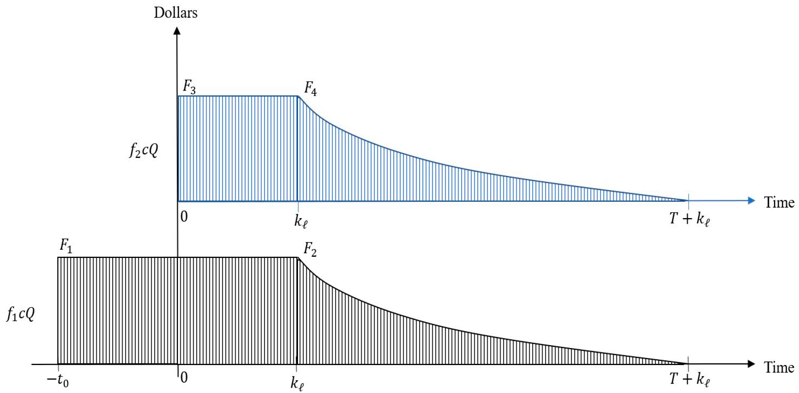
Figure 1. The graphical depiction of advance and cash payments.
Mathematics 12 01033 g001
Figure 2. The graphical depiction of credit payments for Case 1.1.
Mathematics 12 01033 g002
Figure 3. The graphical depiction of credit payments for Case 1.2.
Mathematics 12 01033 g003
Figure 4. The graphical depiction of credit payments for Case 1.3.
Mathematics 12 01033 g004
Figure 5. The graphical depiction of credit payments for Case 2.
Mathematics 12 01033 g005
Figure 6. The graph of P T P 1 ( S , T ) .
Mathematics 12 01033 g006
Figure 7. The graph of P T P 2 ( S , T ) .
Mathematics 12 01033 g007
Figure 8. The graph of P T P 3 ( S , T ) .
Mathematics 12 01033 g008
Figure 9. The graph of P T P 4 ( S , T ) .
Mathematics 12 01033 g009
Figure 10. The graph of P T P 2 ( S , T ) .
Mathematics 12 01033 g010
Figure 11. The graph of P T P 4 ( S , T ) .
Mathematics 12 01033 g011
Table 1. A brief review of the related literature.
ReferencesDemand FunctionPayment TypeCarbon Policy
Chang et al. [43]PriceACCX
Cheng et al. [16]PriceAdvance-CreditCarbon tax
Feng et al. [39]Price, Stock Age, and LevelACCX
Jain et al. [17]ConstantXCap-and-trade, Carbon tax, and Carbon offset
Li and Teng [48]Price, Stock Age, and LevelCashX
Li et al. [51]Price and Stock AgeACCX
Li et al. [52]Price ACCX
Ma et al. [6]Price and FreshnessXCap-and-trade
Mishra et al. [8]Price and Stock XCap-and-trade
Roy and Sana [53])StochasticCreditX
Sabzevar et al. [10]PriceXCap-and-trade
Shi et al. [12]Constant ACCCarbon tax
Shi et al. [45]Time ACCX
Taleizadeh et al. [44]ConstantAdvance-Credit X
Tsao et al. [40]ConstantACCX
Wu et al. [42]ConstantACCX
This paperPrice and Stock AgeACCCap-and-trade and Carbon tax
X: none.
Table 2. Analysis of sensitivity and the trends in each parameter’s impact on the decision variable.
Decision S * T * Q * P T P * T C E *
Parameter
o = 200 65.010.1411153.2411,343.704797.41
o = 250 65.070.1536757.2011,000.904545.60
o = 300 65.120.1653860.7810,684.104342.41
trend
c = 25 59.970.1427662.5613,038.405082.61
c = 30 65.070.1536757.2011,000.904545.60
c = 35 70.180.1655152.259271.164069.54
trend
γ = 0.05 65.020.1543257.4911,059.104536.50
γ = 0.07 65.070.1536757.2011,000.904545.60
γ = 0.09 65.120.1530356.9110,942.804554.47
trend
k u = 0.20 65.140.1539357.1610,965.604536.65
k u = 0.25 65.070.1536757.2011,000.904545.60
k u = 0.30 65.000.1533857.2311,036.904554.96
trend
k l = 0.10 64.960.1503457.1911,061.904563.57
k l = 0.15 65.070.1536757.2011,000.904545.60
k l = 0.20 65.180.1542657.2010,942.604528.62
trend
ρ = 0.3 64.990.1531357.1611,058.504560.09
ρ = 0.4 65.070.1536757.2011,000.904545.60
ρ = 0.5 65.150.1542257.2410,943.404531.09
trend
t 0 = 0.10 65.000.1532557.1811,032.204557.21
t 0 = 0.15 65.070.1536757.2011,000.904545.60
t 0 = 0.20 65.130.1541057.2210,969.604534.00
trend
h = 4 65.000.1544457.5611,028.104535.59
h = 5 65.070.1536757.2011,000.904545.60
h = 6 65.140.1529156.8410,973.904555.57
trend
x = 0.5 65.040.1426152.2310,628.104710.01
x = 0.6 65.070.1536757.2011,000.904545.60
x = 0.7 65.090.1633161.5611,292.904422.22
trend
I p = 0.06 65.020.1536857.2911,019.404548.37
I p = 0.07 65.070.1536757.2011,000.904545.60
I p = 0.08 65.120.1536657.1110,982.404542.85
trend
I e = 0.04 65.130.1542757.2910,959.704531.37
I e = 0.05 65.070.1536757.2011,000.904545.60
I e = 0.06 65.010.1530857.1111,042.204559.84
trend
b = 4 64.870.1532257.4011,075.604191.14
b = 5 65.070.1536757.2011,000.904545.60
b = 6 65.270.1541357.0010,926.704895.31
trend
o e = 350 65.060.1512356.4411,067.204260.84
o e = 400 65.070.1536757.2011,000.904545.60
o e = 450 65.080.1560757.9410,935.604822.01
trend
h e = 2 65.050.1538257.2711,006.304516.39
h e = 3 65.070.1536757.2011,000.904545.60
h e = 4 65.080.1535257.1310,995.504574.74
trend
c e = 0.1 64.500.1428654.6511,070.204790.71
c e = 0.2 65.070.1536757.2011,000.904545.60
c e = 0.3 65.640.1640859.4410,954.504333.59
trend
Note: ↗ is increasing; ↘ is decreasing.
Disclaimer/Publisher’s Note: The statements, opinions and data contained in all publications are solely those of the individual author(s) and contributor(s) and not of MDPI and/or the editor(s). MDPI and/or the editor(s) disclaim responsibility for any injury to people or property resulting from any ideas, methods, instructions or products referred to in the content.

Share and Cite

MDPI and ACS Style

Chang, C.-T.; Tseng, Y.-T. The Impacts of Payment Schemes and Carbon Emission Policies on Replenishment and Pricing Decisions for Perishable Products in a Supply Chain. Mathematics 2024, 12, 1033. https://doi.org/10.3390/math12071033

AMA Style

Chang C-T, Tseng Y-T. The Impacts of Payment Schemes and Carbon Emission Policies on Replenishment and Pricing Decisions for Perishable Products in a Supply Chain. Mathematics. 2024; 12(7):1033. https://doi.org/10.3390/math12071033

Chicago/Turabian Style

Chang, Chun-Tao, and Yao-Ting Tseng. 2024. "The Impacts of Payment Schemes and Carbon Emission Policies on Replenishment and Pricing Decisions for Perishable Products in a Supply Chain" Mathematics 12, no. 7: 1033. https://doi.org/10.3390/math12071033

APA Style

Chang, C. -T., & Tseng, Y. -T. (2024). The Impacts of Payment Schemes and Carbon Emission Policies on Replenishment and Pricing Decisions for Perishable Products in a Supply Chain. Mathematics, 12(7), 1033. https://doi.org/10.3390/math12071033

Note that from the first issue of 2016, this journal uses article numbers instead of page numbers. See further details here.

Article Metrics