
Method for the Statistical Analysis of the Signals Generated by an Acquisition Card for Pulse Measurement


Abstract
1. Introduction
1.1. Methods for Measuring Pulse
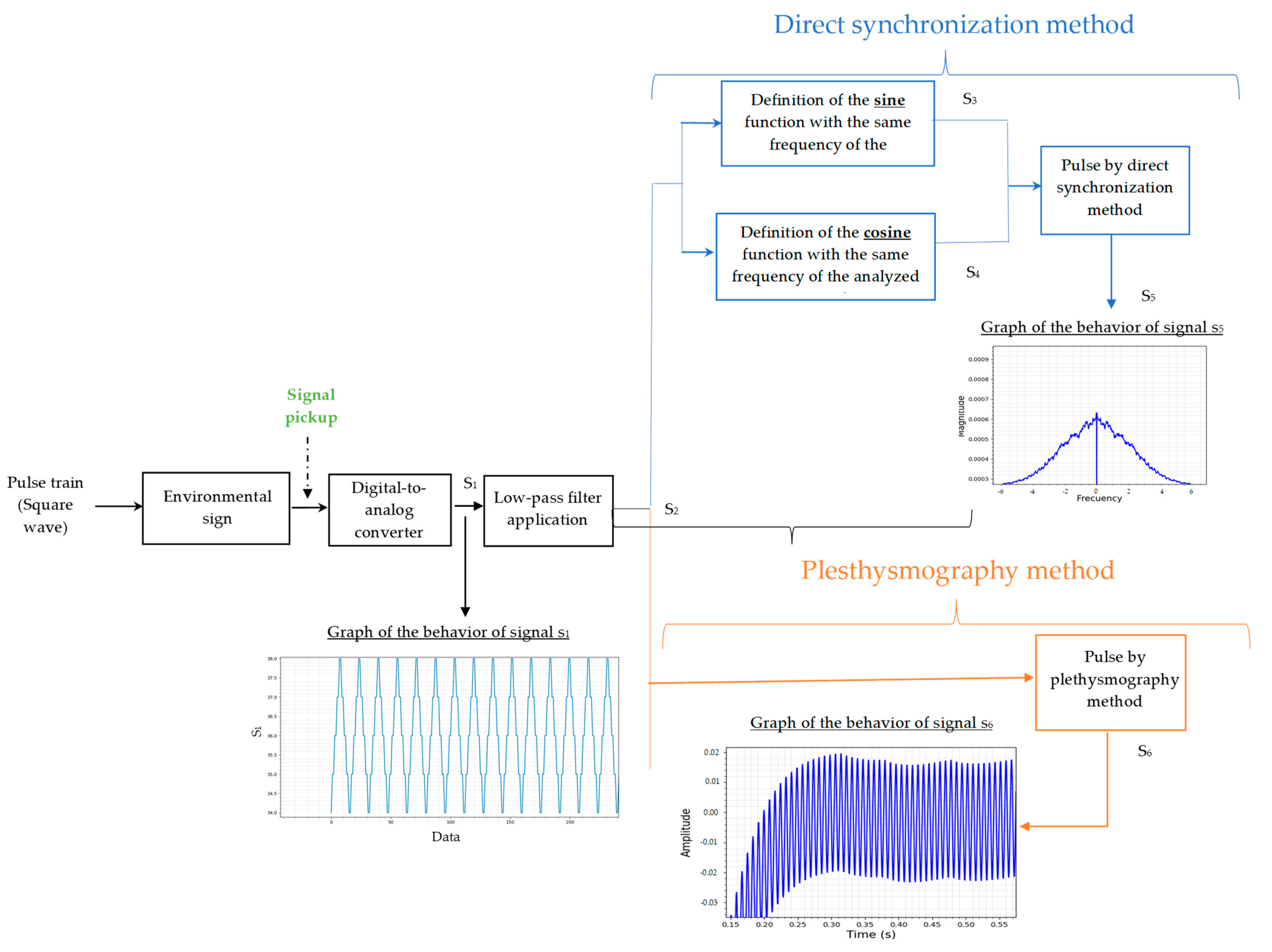
1.2. Pulse by the Synchronous Demodulation
1.3. Pulse by Plethysmography Method
1.4. Descriptive Statistics
- The mean, which is calculated from the sum of each of the signal data divided by the total data; see Equation (1):
- The standard deviation (σ) is defined as a measure of the dispersion by which points differ from the mean. And in which a low value indicates that the points are very close to the mean, while a high deviation shows that the points are spread over a larger range of values. σ is calculated from Equation (2):
- The variation coefficient (CV) is used to compare data sets belonging to different populations, allowing a measure of dispersion that eliminates possible distortions of the means of two or more populations. CV is calculated from Equation (3):
- A scatterplot is one of the most powerful yet simple visual plots available. Scatterplots can also indicate the existence of patterns or groups of clusters in the data and identify outliers in the data [31].
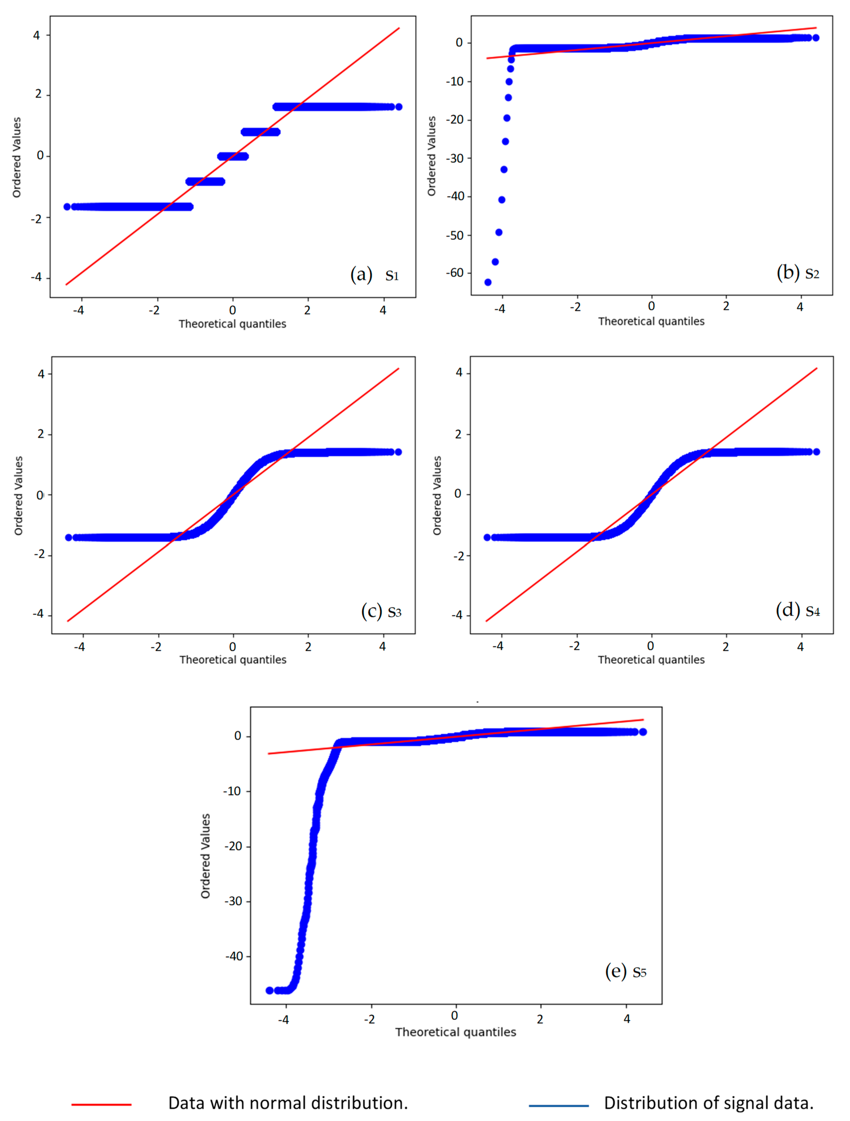
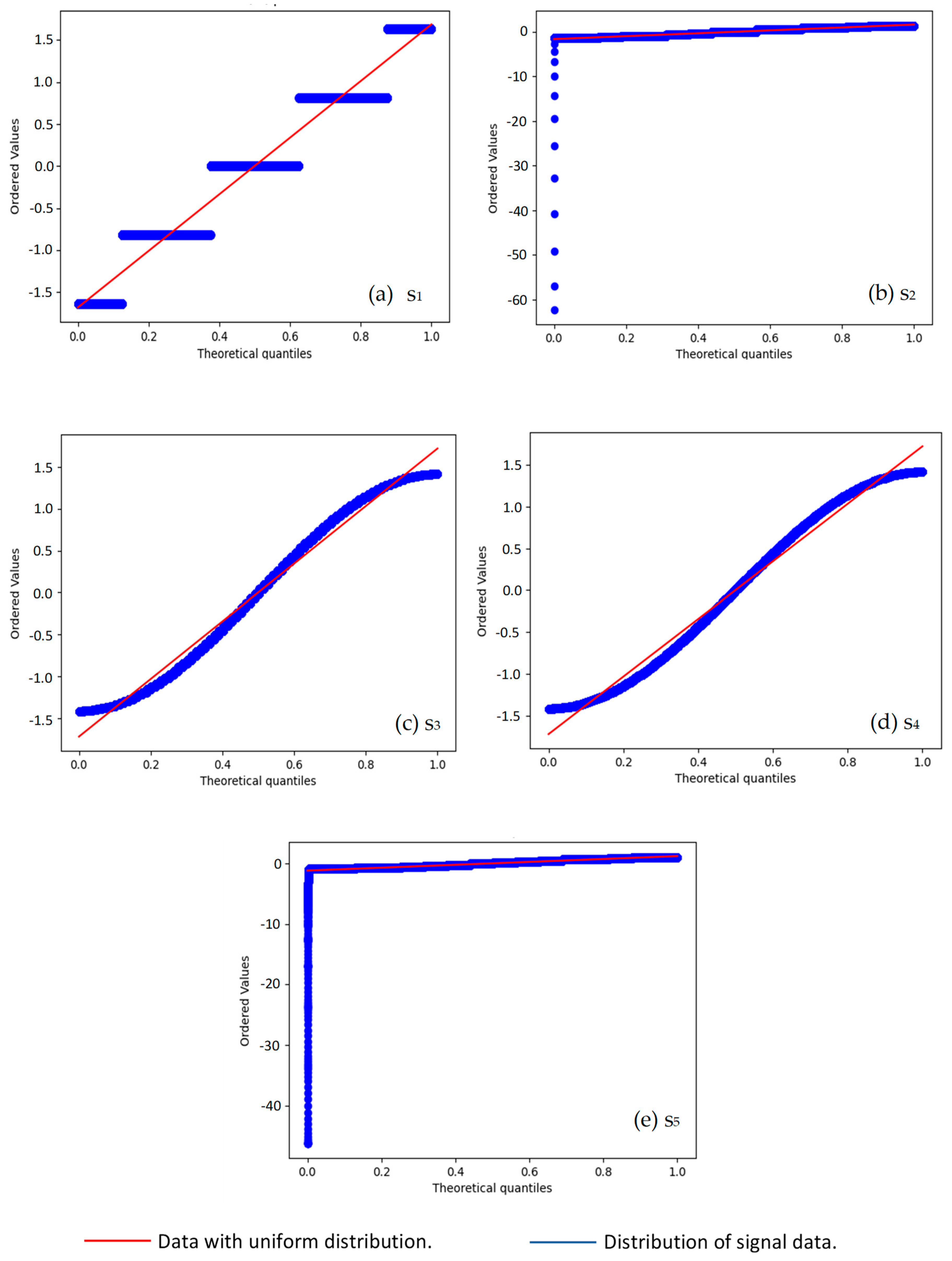
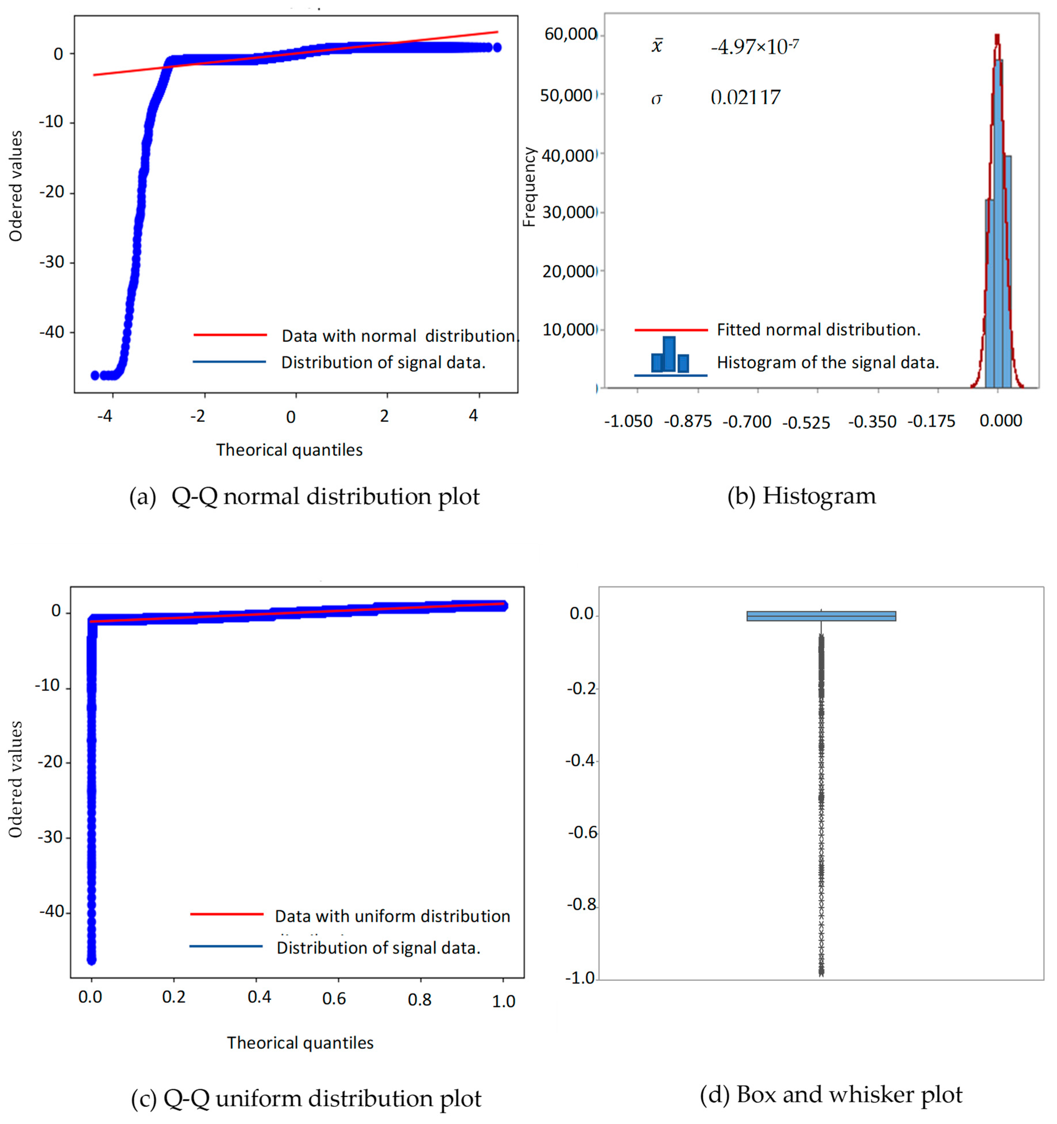
- A quantile-to-quantile plot (Q-Q plot) is a graph that tests the conformity between the empirical distribution and the given theoretical distribution. A Q-Q plot is used to verify if data follow a particular distribution or if two given data sets have the same distribution. If the distributions are the same, the graph is a line. The further the obtained results are from the 45° diagonal, the further the empirical distribution from the theoretical one. The extreme points have a greater variability than those in the center of the distribution [32].
1.5. Augmented Dickey–Fuller Test
1.6. Hurst Exponent
1.7. Metrics to Measure the Error between Two Series
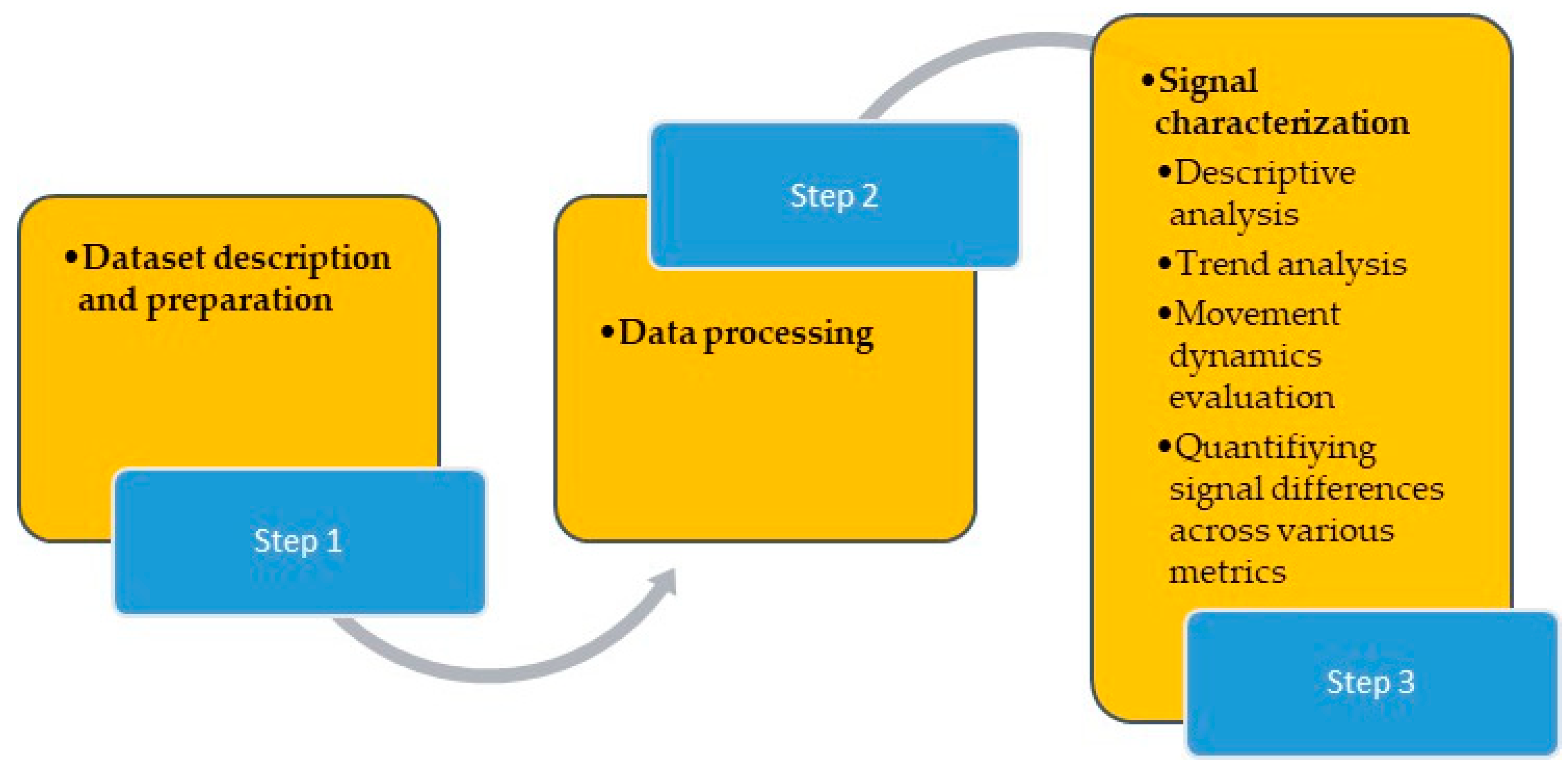
2. Statistical Method for Analysis of Signal
- Step 1. Dataset description and preparation
- Step 2. Data processing
- Step 3. Signal characterization
3. Results
4. Discussion
- It is easy to use and interpret;
- Allows you to describe the signals in a simple way;
- Enables developers to have a tuning tool during the development stages;
- It is an alternative to evaluate the function of systems that emit, process, or collect signals before being implemented in the system or ecosystem of the study individuals;
- As it is a methodology made up of solid statistical tools, its efficient use is supported.
- The metric evaluated to measure the error between two series, MAPE and MPE, are not satisfactory when taking values such as 0, or very small ones; therefore, is not recommended in this scenario. And ME values vary in sign due to the order in which the signals were compared. Therefore, evaluating it once in the series comparison is enough.
5. Conclusions
Author Contributions
Funding
Data Availability Statement
Acknowledgments
Conflicts of Interest
Abbreviations
| Notation | Interpretation |
| AC | Acquisition card |
| Mean | |
| Standard deviation | |
| CV | Coefficient of variation |
| ADF | Augmented Dickey–Fuller test |
| H | Hurst exponent |
| MSE | Mean-squared error |
| RMSE | Root-mean-square error |
| MAE | Mean absolute error |
| ME | Mean error |
| MAPE | Mean absolute percentage error |
| MPE | Mean percentage error |
| X | Each value in the sample |
| N | Amount of data |
| Error between two-time series (residual) | |
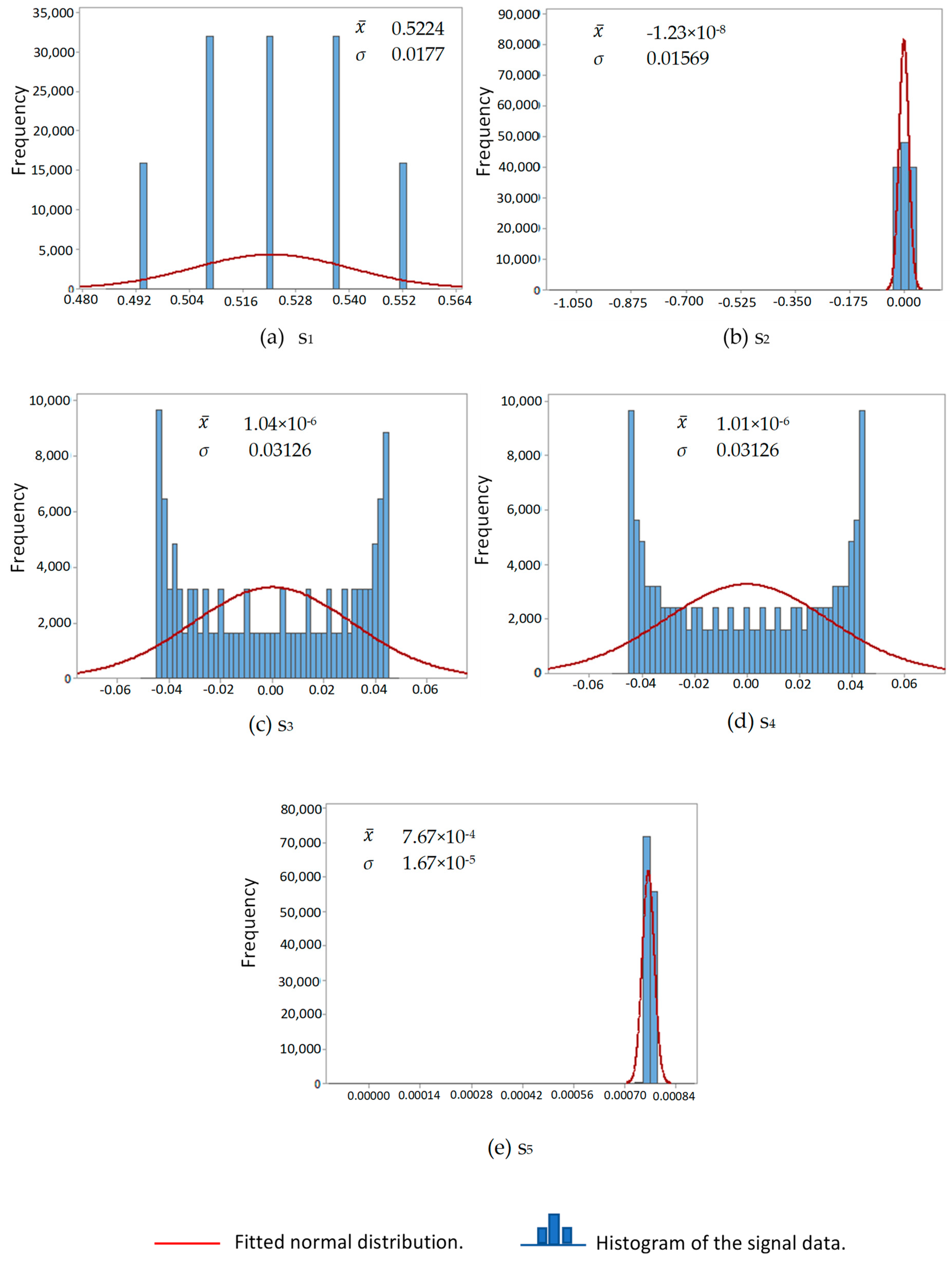
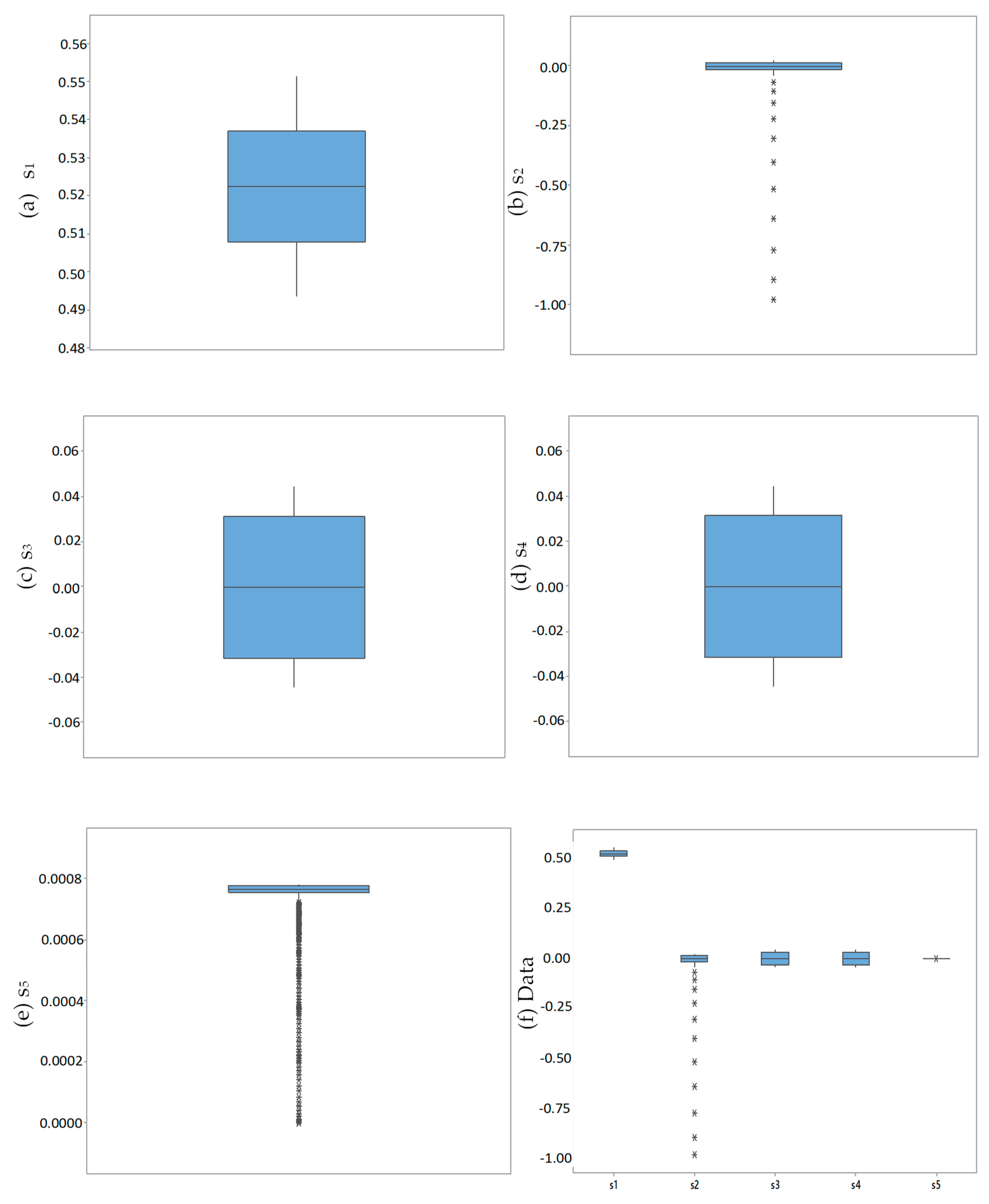
| s1 | Digital signal |
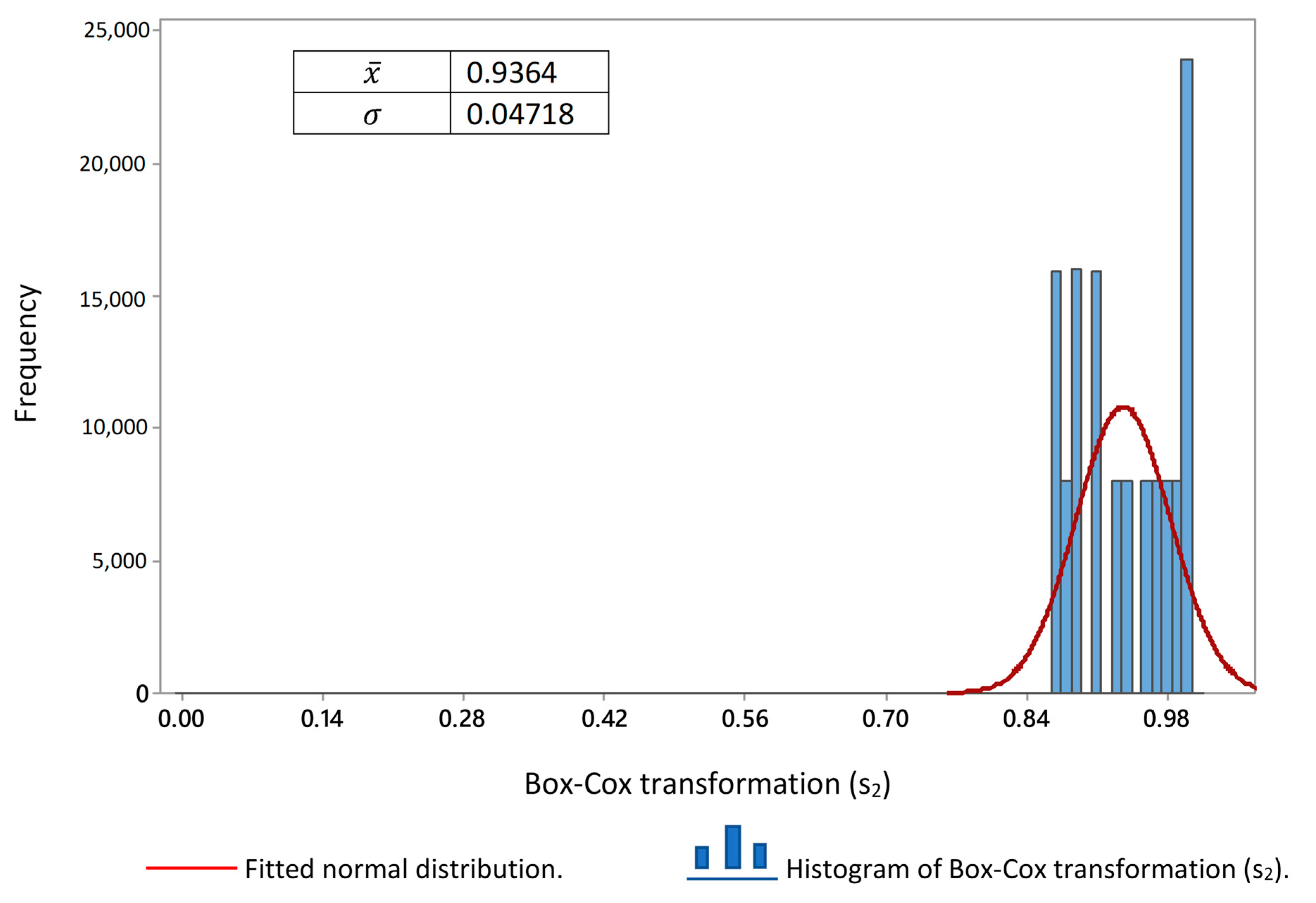
| s2 | Signal after that the pass filter was applied |
| s3 | Sine function with the same frequency of the analyzed signal |
| s4 | Cosine function with the same frequency of the analyzed signal |
| s5 | Pulse by direct synchronization method |
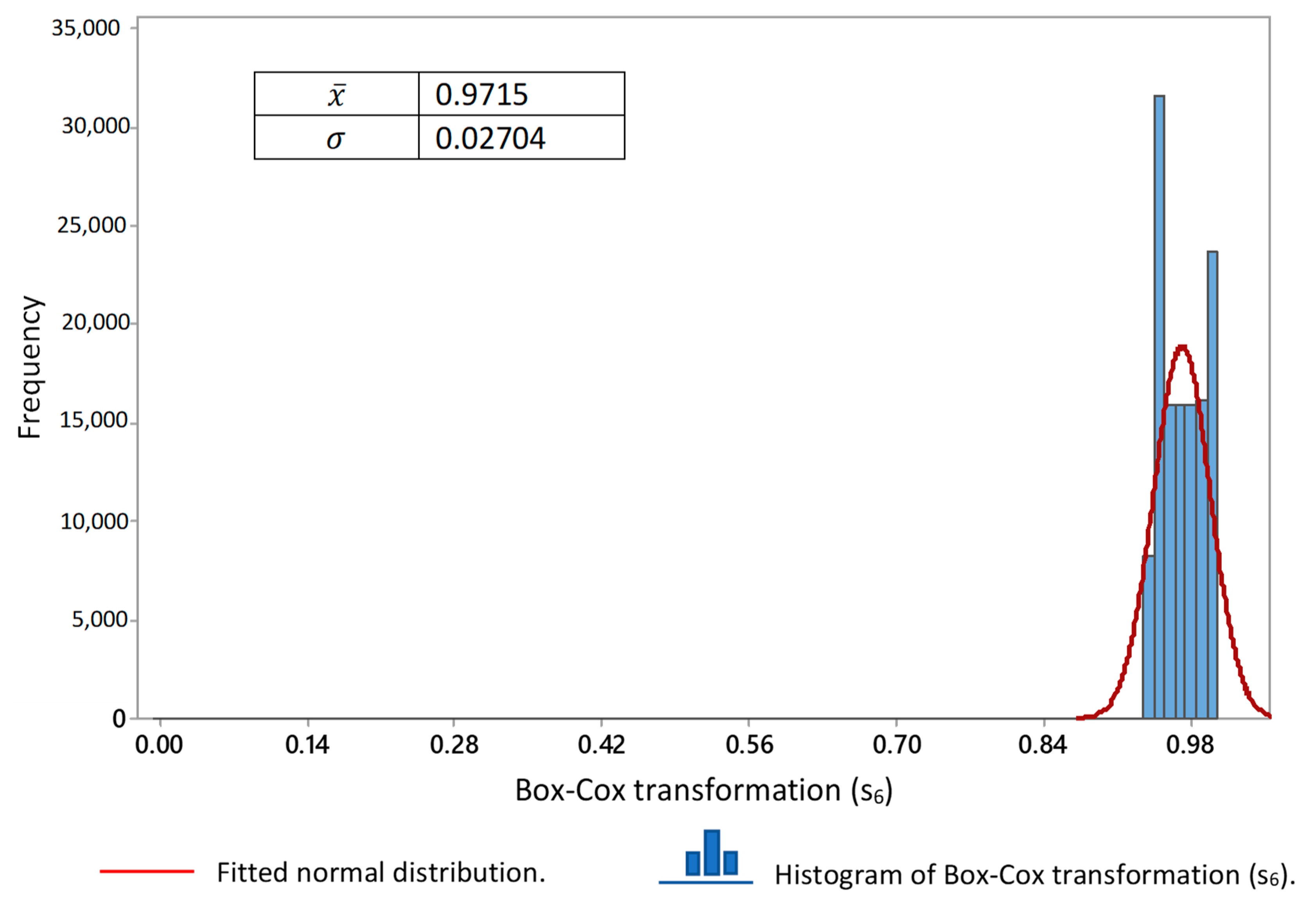
| s6 | Pulse by plethysmography method |
References
- Wu, W.; Ling, B.W.K.; Li, R.; Lin, Z.; Liu, Q.; Shao, J.; Ho, C.Y.-F. Classification Approach for Attention Assessment via Singular Spectrum Analysis Based on Single-Channel Electroencephalograms. Sensors 2023, 23, 761. [Google Scholar] [CrossRef]
- Lambert Cause, J.; Solé Morillo, Á.; da Silva, B.; García-Naranjo, J.C.; Stiens, J. Novel Multi-Parametric Sensor System for Comprehensive Multi-Wavelength Photoplethysmography Characterization. Sensors 2023, 23, 6628. [Google Scholar] [CrossRef] [PubMed]
- Centracchio, J.; Parlato, S.; Esposito, D.; Bifulco, P.; Andreozzi, E. ECG-Free Heartbeat Detection in Seismocardiography Signals via Template Matching. Sensors 2023, 23, 4684. [Google Scholar] [CrossRef] [PubMed]
- Martínez-Suárez, F.; García-Limón, J.A.; Baños-Bautista, J.E.; Alvarado-Serrano, C.; Casas, O. Low-Power Long-Term Ambulatory Electrocardiography Monitor of Three Leads with Beat-to-Beat Heart Rate Measurement in Real Time. Sensors 2023, 23, 8303. [Google Scholar] [CrossRef] [PubMed]
- Romagnoli, S.; Ripanti, F.; Morettini, M.; Burattini, L.; Sbrollini, A. Wearable and Portable Devices for Acquisition of Cardiac Signals while Practicing Sport: A Scoping Review. Sensors 2023, 23, 3350. [Google Scholar] [CrossRef] [PubMed]
- Moraes, J.L.; Rocha, M.X.; Vasconcelos, G.G.; Vasconcelos Filho, J.E.; De Albuquerque, V.H.C.; Alexandria, A.R. Advances in Photoplethysmography Signal Analysis for Biomedical Applications. Sensors 2018, 18, 1894. [Google Scholar] [CrossRef] [PubMed]
- Park, J.; Hong, K. Robust Pulse Rate Measurements from Facial Videos in Diverse Environments. Sensors 2022, 22, 9373. [Google Scholar] [CrossRef]
- Chi, Y.M.; Cauwenberghs, G. Wireless Non-contact EEG/ECG Electrodes for Body Sensor Networks. In Proceedings of the International Conference on Body Sensor Networks, Singapore, 7–9 June 2010; pp. 297–301. [Google Scholar] [CrossRef]
- Yang, Z.; Mitsui, K.; Wang, J.; Saito, T.; Shibata, S.; Mori, H.; Ueda, G. Non-Contact Heart-Rate Measurement Method Using Both Transmitted Wave Extraction and Wavelet Transform. Sensors 2021, 21, 2735. [Google Scholar] [CrossRef] [PubMed]
- Wang, H.; Du, F.; Zhu, H.; Zhu, X.; Cao, Q. Hear rate measurement method based on wavelet transform noise reduction for low power millimeter wave radar platform. J. Phys. 2023, 2469, 012026. [Google Scholar] [CrossRef]
- Poh, M.Z.; McDuff, D.J.; Picard, R.W. Non-contact, automated cardiac pulse measurements using video imaging and blind source separation. Opt. Express 2010, 18, 10762–10774. [Google Scholar] [CrossRef]
- Chi, R.; Li, H.; Shen, D.; Hou, Z.; Huang, B. Enhanced P-Type Control: Indirect Adaptive Learning from Set-Point Updates. IEEE 2023, 12, 3242. [Google Scholar] [CrossRef]
- Kalarickel Ramakrishnan, P.; Westwood, T.; Magalhães Gouveia, T.; Taani, M.; de Jager, K.; Murdoch, K.; Orlov, A.A.; Ozhgibesov, M.S.; Propodalina, T.V.; Wojtowicz, N. Capacitance Estimation for Electrical Capacitance Tomography Sensors Using Digital Processing of Time-Domain Voltage Response to Single-Pulse Excitation. Electronics 2023, 12, 3242. [Google Scholar] [CrossRef]
- Darwish, A.; Ricci, M.; Zidane, F.; Vasquez, J.A.T.; Casu, M.R.; Lanteri, J.; Migliaccio, C.; Vipiana, F. Physical Contamination Detection in Food Industry Using Microwave and Machine Learning. Electronics 2022, 11, 3115. [Google Scholar] [CrossRef]
- Muto, V.; Andreozzi, E.; Cappelli, C.; Centracchio, J.; Di Meo, G.; Esposito, D.; Bifulco, P.; De Caro, D. Real-Time Implementation of a Frequency Shifter for Enhancement of Heart Sounds Perception on VLIW DSP Platform. Electronics 2023, 12, 4359. [Google Scholar] [CrossRef]
- Lee, S.-H.; Cheng, C.H.; Lin, C.C.; Huang, Y.F. PSO-Based Target Localization and Tracking in Wireless Sensor Networks. Electronics 2023, 12, 905. [Google Scholar] [CrossRef]
- Di Patrizio Stanchieri, G.; Saleh, M.; De Marcellis, A.; Ibrahim, A.; Faccio, M.; Valle, M.; Palange, E. FPGA-Based Tactile Sensory Platform with Optical Fiber Data Link for Feedback Systems in Prosthetics. Electronics 2023, 12, 627. [Google Scholar] [CrossRef]
- Colaiuda, D.; Leoni, A.; Ferri, G.; Stornelli, V. A Second Order 1.8–1.9 GHz Tunable Active Band-Pass Filter with Improved Noise Performances. Electronics 2022, 11, 2781. [Google Scholar] [CrossRef]
- Bautista López, R.Z.; Yáñez Mendiola, J.; Sicard González, M.T. Branchial Motion Assessment in Abalone Using Photoplethysmography. Aquac. Res. 2023, 2023, 6672198. [Google Scholar] [CrossRef]
- Bruning, J.H.; Herriott, D.R.; Gallagher, J.E.; Rosenfeld, D.P.; White, A.D.; Brangaccio, D.J. Digital Wavefront Measuring Interferometer for Testing Optical Surfaces and Lenses. Appl. Opt. 1974, 13, 2693–2703. [Google Scholar] [CrossRef]
- Optical Shop Testing, 3rd ed.; Malacara, D., Ed.; Wiley Series in Pure and Applied Optics; John Wiley & Sons: Hoboken, NJ, USA, 2007. [Google Scholar]
- Zurich Instruments. Principles of Lock-In Detection and the State of the Art. 2016. Available online: https://www.zhinst.com/sites/default/files/documents/2020-06/zi_whitepaper_principles_of_lock-in_detection.pdf (accessed on 21 October 2023).
- Shenoy, R.; Ramakrishna, J.; Jeffrey, K. A simple and inexpensive two channel boxcar integrator. Pramana 1979, 13, 1–7. [Google Scholar] [CrossRef]
- Efthymiou, S.; Ozanyan, K.B. Pulse Detection by Gated Synchronous Demodulation. IEEE Sens. J. 2013, 13, 3349–3360. [Google Scholar] [CrossRef]
- Kyriacou, P.; Allen, J. Photoplethysmography—Technology, Signal Analysis and Applications, 1st ed.; Academic Press: Cambridge, MA, USA, 2021; pp. 401–439. [Google Scholar]
- Addison, P.S.; Watson, J.N. Secondary transform decoupling of shifted nonstationary signal modulation components: Application to photoplethysmography. Int. J. Wavelets Multiresolution Inf. Process. 2004, 2, 43–57. Available online: https://www.worldscientific.com/doi/10.1142/S0219691304000329 (accessed on 21 October 2023). [CrossRef]
- Karlen, W.; Raman, S.; Ansermino, J.M.; Dumont, G.A. Multiparameter respiratory rate estimation from the photoplethysmogram. IEEE Trans. Bio-Med. Eng. 2013, 60, 1946–1953. [Google Scholar] [CrossRef] [PubMed]
- Stearns, S.D.; Hush, D.R. Digital Signal Processing with Examples in Matlab(r), 2nd ed.; CRC Press: Boca Raton, FL, USA, 2011. [Google Scholar]
- Akselrod, S.; Gordon, D.; Ubel, F.A.; Shannon, D.C.; Berger, A.C.; Cohen, R.J. Power spectrum analysis of heart rate fluctuation: A quantitative probe of beat-to-beat cardiovascular control. Science 1981, 213, 220–222. [Google Scholar] [CrossRef]
- Anderson, R.R.; Parrish, J.A. The Optics of Human Skin. J. Investig. Dermatol. 1981, 77, 13–19. [Google Scholar] [CrossRef] [PubMed]
- Hertzman, A.B. The blood supply of various skin areas as estimated by the photoelectric plethysmograph. Am. J. Physiol. -Leg. Content 1938, 124, 328–340. [Google Scholar] [CrossRef]
- Montgomery, D.C. Applied Statistics and Probability for Engineers, 13th ed.; Wiley and Sons Inc.: Hoboken, NJ, USA, 2003. [Google Scholar]
- Mendenhall, W.; Beaver, R.J.; Beaver, B.M. Introduction to Probability and Statistics, 13th ed.; Brooks/COLE Cengage Learning: Belmont, CA, USA, 2009. [Google Scholar]
- Vijay, K.; Bala, D. Data Science Concepts and Practice, 2nd ed.; Morgan Kaufmann Publishers an Imprint of Elsevier: Burlington, MA, USA, 2019. [Google Scholar]
- Anonymous Q-Q Plot (Quantile to Quantile Plot). In The Concise Encyclopedia of Statistics; Springer: New York, NY, USA, 2008. [CrossRef]
- Mushtaq, R. Augmented Dickey Fuller Test. 2011. Available online: https://papers.ssrn.com/sol3/papers.cfm?abstract_id=1911068 (accessed on 21 October 2023).
- Minitab. 2021. Available online: https://www.minitab.com (accessed on 21 October 2023).
- Delgadillo, R.O.; Leos, R.J.A.; Ramírez, M.P.; Valdez, C.R. Fractal analysis of time series of anomalies of bean variables in Mexico. Sci. Ergo Sum 2015, 22, 233–241. [Google Scholar]
- Aguilar, R. The Hurst coefficient and the parameter α-stable for financial series analysis. Application to the Mexican exchange market. Account. Adm. 2014, 59, 149–173. Available online: https://www.redalyc.org/articulo.oa?id=39529381007 (accessed on 21 October 2023).
- Luengas, D.D.; Ardila, R.E.; Moreno, T.J.F. Metodología e interpretación del coeficiente de Hurts. ODEON 2010, 5, 265–290. Available online: https://www.redalyc.org/pdf/532/53220677008.pdf (accessed on 21 October 2023).
- Sanders, N.R. Measuring forecast accuracy: Some practical suggestions. Prod. Inventory Manag. J. 1997, 38, 46. Available online: https://www.proquest.com/openview/a4ac156f78d9183cd890d8cedc15ed53/1?pq-origsite=gscholar&cbl=36911 (accessed on 21 October 2023).
- Jierula, A.; Wang, S.; OH, T.-M.; Wang, P. Study on Accuracy Metrics for Evaluating the Predictions of Damage Locations in Deep Piles Using Artificial Neural Networks with Acoustic Emission Data. Appl. Sci. 2021, 11, 2314. [Google Scholar] [CrossRef]
- St-Aubin, P.; Agard, B. Precision and Reliability of Forecasts Performance Metrics. Forecasting 2022, 4, 882–903. [Google Scholar] [CrossRef]
- Nkongolo, M. Using ARIMA to Predict the Growth in the Subscriber Data Usage. Eng 2023, 4, 92–120. [Google Scholar] [CrossRef]
- Menculini, L.; Marini, A.; Proietti, M.; Garinei, A.; Bozza, A.; Moretti, C.; Marconi, M. Comparing Prophet and Deep Learning to ARIMA in Forecasting Wholesale Food Prices. Forecasting 2021, 3, 644–662. [Google Scholar] [CrossRef]
- Ampountolas, A. Comparative Analysis of Machine Learning, Hybrid, and Deep Learning Forecasting Models: Evidence from European Financial Markets and Bitcoins. Forecasting 2023, 5, 472–486. [Google Scholar] [CrossRef]
- Promodel. 2016. Available online: https://promodel.com.mx/ (accessed on 21 October 2023).
- Karjanto, N. Bright Soliton Solution of the Nonlinear Schrödinger Equation: Fourier Spectrum and Fundamental Characteristics. Mathematics 2022, 10, 4559. [Google Scholar] [CrossRef]


| Development | Description | Advantages | Disadvantages | Year/References |
|---|---|---|---|---|
| Cardiac pulse detection by a pulse train using the synchronous Demodulation Technique. | In this document, the operating principle is presented, together with the mathematical demonstration of the theory on which the method for the treatment and recovery of the heart rate signal is based. | The method is presented in mathematical form. | The number of dates must be expanded. | 2023/Project with reference to number 0000000287237 CB-2016-01 |
| This method uses a low-power millimeter wave radar system. | It uses a low-power millimeter wave radar system with a transmission power of less than 6 dBm. | In a 20 min monitoring experiment, 96.96% accuracy is reached by this method. | These low-power devices make it impossible to maintain the echo intensity at an optimal level, making accurate and reliable monitoring. | 2023/[10] |
| Use of facial videos. | Robust pulse rate measurements from facial videos in diverse environments. | The method stably detects faces by removing high-frequency components of face coordinate signals derived from noise factors. | The method uses the average of interval values between detected peak points. | 2022/[7] |
| Several capacitive coupling methods. | The system is composed of a set of capacitive electrodes manufactured on a standard printed circuit board. | The system may cause inconvenience, such as foreign body sensations. | This presents weak detection signals. | 2021/[8] |
| The method is to use microwave or millimeter wave Doppler radar as a non-contact hear-rate measurement system. | This method uses ultra-wideband or millimeter wave signals and focuses on detection on the skin surface. | This method can obtain information about the diastole and systole of the heart, as well as the surface of the skin. | Their effectiveness in vehicle environments remains unclear. | 2021/[9] |
| Non-contact, automated cardiac pulse measurements using video imaging and blind source separation. | The authors used bland-Altman and correlation analysis, to compare the cardiac pulse rate extracted from videos recorded by a basic webcam to an FDA-approved finger blood volume pulse sensor. | High precision and correlation were achieved (even with the presence of motion). | It is possible that the linearity assumed is not representative of the true underlying mixture in the signals. | 2010/[11] |
| Characteristics | Statistical Parameters of Tendency and Dispersion |
|---|---|
| Descriptive statistical analysis | Type of data distribution, Q-Q plots, Histograms, Box and , σ, CV, |
| Trend analysis | ADF |
| Dynamics of movement | H |
| Metric in measuring the error | MSE, RMSE, MAE, ME, MAPE, MPE, residual graphs |
| Signal | Minimum Value | Box-Cox Transformation |
|---|---|---|
| S2 | −0.98 | |
| S5 | −0.00000000001 | |
| S6 | −0.98 |
| Signal | CV-Value | Detected Distribution |
|---|---|---|
| s1 | 3.4 | Normal Lognormal Uniform |
| s2 | −127 × 106 | Uniform Normal Lognormal Exponential (oscillating) |
| s3 | 3 × 10⁶ | Uniform Normal Lognormal Exponential (oscillating) |
| s4 | 3 × 10⁶ | Normal Lognormal Uniform Exponential (oscillating) |
| s5 | 2.16 | Uniform Normal Lognormal Exponential (oscillating) |
| Signal | ADF Calculated | ADF Result | H Calculated | H Results |
|---|---|---|---|---|
| s1 | Test: −113.15556052161811 p-value: 0.0 Critical values: {‘1%’: −3.4304010901041226, ‘5%’: −2.8615625810800256, ‘10%’: −2.566782019109249} | s1 is stationary | 0.01 | The memory of s1 is anti-persistent. |
| s2 | Test: −1068.923788266477 p-value: 0.0 Critical values: {‘1%’: −3.4304010905032816, ‘5%’: −2.8615625812564462, ‘10%’: −2.566782019203152} | s2 is stationary | 0.32 | The memory of s2 is anti-persistent. |
| s3 | Test: −13585028329382.6 p-value: 0.0 Critical values: {‘1%’: −3.4304010905032816, ‘5%’: −2.8615625812564462, ‘10%’: −2.566782019203152} | s3 is stationary | 0.00 | The memory of s3 is anti-persistent. |
| s4 | Test: −13583953241809.928 p-value: 0.0 Critical values: {‘1%’: −3.4304010905032816, ‘5%’: −2.8615625812564462, ‘10%’: −2.566782019203152} | s4 is stationary | 0.00 | The memory of s4 is anti-persistent. |
| s5 | Test: −311.9388497424053 p-value: 0.0 Critical values: {‘1%’: −3.4304010913016176, ‘5%’: −2.8615625816092964, ‘10%’: −2.566782019390962} | s5 is stationary | 0.33 | The memory of s5 is anti-persistent. |
| Statistical | Signal | ||||
|---|---|---|---|---|---|
| s1 | s2 | s3 | s4 | s5 | |
| s1 | 0.273 | 0.274 | 0.274 | 0.272 | |
| 0.522 | 0.523 | 0.523 | 0.523 | ||
| 0.522 | 0.522 | 0.522 | 0.522 | ||
| 0.522 | 0.522 | 0.522 | 0.521 | ||
| s2 | 0.273 | 0.001 | 0.001 | 0.0002 | |
| 0.522 | 0.034 | 0.035 | 0.016 | ||
| 0.522 | 0.029 | 0.029 | 0.013 | ||
| −0.522 | −1.052 × 10⁻⁶ | −1.022 × 10⁻⁶ | −7.77 × 10⁻⁴ | ||
| s3 | 0.274 | 0.001 | 0.002 | 0.001 | |
| 0.523 | 0.034 | 0.044 | 0.031 | ||
| 0.522 | 0.029 | 0.039 | 0.028 | ||
| −0.522 | 1.052 × 10⁻⁶ | −3.037 × 10⁻⁸ | −7.65 × 10⁻⁴ | ||
| s4 | 0.274 | 0.001 | 0.002 | 0.001 | |
| 0.523 | 0.035 | 0.044 | 0.031 | ||
| 0.522 | 0.029 | 0.039 | 0.028 | ||
| −0.522 | 1.022 × 10⁻⁶ | 3.037 ×10⁻⁸ | −7.65 × 10⁻⁴ | ||
| s5 | 0.272 | 0.0002 | 0.001 | 0.001 | |
| 0.523 | 0.016 | 0.031 | 0.031 | ||
| 0.522 | 0.013 | 0.028 | 0.028 | ||
| −0.521 | 7.77 × 10⁻⁴ | 7.65 × 10⁻⁴ | 7.65 × 10⁻⁴ | ||
| Statistical | Signal | ||||
|---|---|---|---|---|---|
| s1 | s2 | s3 | s4 | s5 | |
| s1 | 9966.33 | 4950.28 | DIV/0 | DIV/0 | |
| 100.02 | 99.99 | 99.99 | 99.85 | ||
| s2 | 100.02 | 175.08 | DIV/0 | DIV/0 | |
| 9966.23 | 547.6 | 547.5 | 100.25 | ||
| s3 | 99.99 | 547.6 | +DIV/0 | DIV/0 | |
| 4650.28 | 175.08 | 402.7 | 101.23 | ||
| s4 | 99.99 | 547.5 | 402.7 | DIV/0 | |
| DIV/0 | DIV/0 | DIV/0 | DIV/0 | ||
| s5 | 99.85 | 100.25 | 101.73 | DIV/0 | |
| DIV/0 | DIV/0 | DIV/0 | DIV/0 | ||
| Signal | ADF Calculated | ADF Result | H Calculated | H Results |
|---|---|---|---|---|
| s6 | Test: −311.93884974369644 p-value: 0.0 Critical values {‘1%’: −3.4304010913016176, ‘5%’: −2.8615625816092964, ‘10%’: −2.566782019390962} | s6 is stationary | 0.33 | The memory of s1 is anti-persistent. |
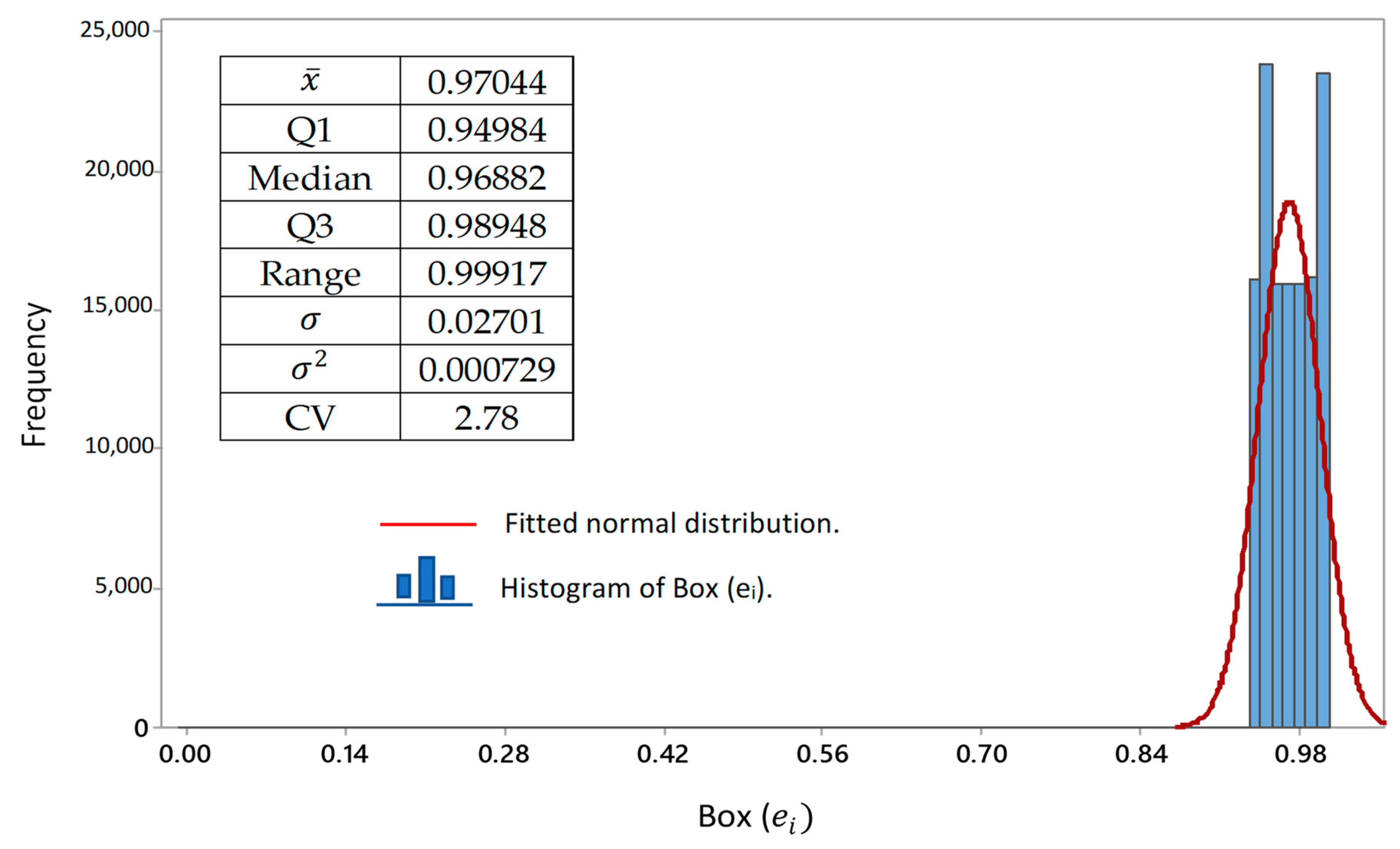
| Characteristic | Pulse by Synchronization Method (s5) | Pulse by Plethysmography Method (s6) | ||||
|---|---|---|---|---|---|---|
| Descriptive Analysis | Statistical | Value | Statistical | Value | ||
| 7.67 × 10⁻⁴ | −4.97 × 10⁻⁷ | |||||
| σ | 1.67 × 10⁻⁵ | σ | 0.02117 | |||
| CV | 2.16 | CV | Non-robust | |||
| Detected distribution | Initial data | Lognormal Normal Uniform | Detected distribution | Initial data | Lognormal Normal Uniform | |
| Central data | Uniform Normal Lognormal Exponential | Central data | Uniform Normal Lognormal Exponential | |||
| Final data | Uniform Normal Lognormal | Final data | Uniform Normal Lognormal | |||
| Distribution dates | Box and whisker plot shows outlier data in the bottom tail | Distribution dates | Box and whisker plot shows outlier data in the bottom tail | |||
| Trend analysis | Stationary | Stationary | ||||
| Dynamics of movement | Anti-persistent (The signals have pink noise) | Anti-persistent (The signals have pink noise) | ||||
| Measuring the error | Error | Value | ||||
| MSE | 0.0004 | |||||
| RMSE | 0.021 | |||||
| MAE | 0.013 | |||||
| ME | −7.67 × 10⁻⁴ | |||||
| MAPE | DIV/0 | |||||
| MPE | 102.86 | |||||
Disclaimer/Publisher’s Note: The statements, opinions and data contained in all publications are solely those of the individual author(s) and contributor(s) and not of MDPI and/or the editor(s). MDPI and/or the editor(s) disclaim responsibility for any injury to people or property resulting from any ideas, methods, instructions or products referred to in the content. |
© 2024 by the authors. Licensee MDPI, Basel, Switzerland. This article is an open access article distributed under the terms and conditions of the Creative Commons Attribution (CC BY) license (https://creativecommons.org/licenses/by/4.0/).
Share and Cite
Pantoja-Pacheco, Y.V.; Yáñez-Mendiola, J. Method for the Statistical Analysis of the Signals Generated by an Acquisition Card for Pulse Measurement. Mathematics 2024, 12, 923. https://doi.org/10.3390/math12060923
Pantoja-Pacheco YV, Yáñez-Mendiola J. Method for the Statistical Analysis of the Signals Generated by an Acquisition Card for Pulse Measurement. Mathematics. 2024; 12(6):923. https://doi.org/10.3390/math12060923
Chicago/Turabian StylePantoja-Pacheco, Yaquelin Verenice, and Javier Yáñez-Mendiola. 2024. "Method for the Statistical Analysis of the Signals Generated by an Acquisition Card for Pulse Measurement" Mathematics 12, no. 6: 923. https://doi.org/10.3390/math12060923
APA StylePantoja-Pacheco, Y. V., & Yáñez-Mendiola, J. (2024). Method for the Statistical Analysis of the Signals Generated by an Acquisition Card for Pulse Measurement. Mathematics, 12(6), 923. https://doi.org/10.3390/math12060923