

A Modified Cure Rate Model Based on a Piecewise Distribution with Application to Lobular Carcinoma Data

 , ,
, ,  and
and 
Abstract
1. Motivation
2. Background
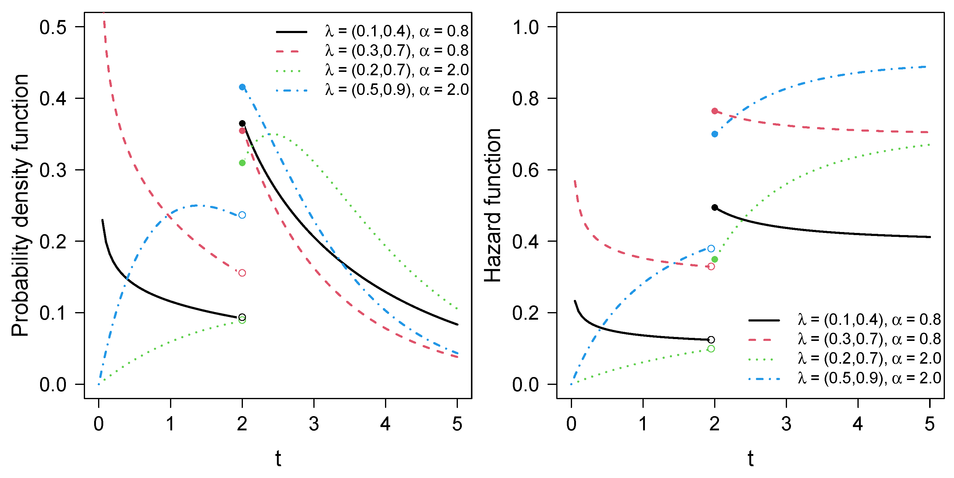
2.1. PPE Distribution
- For , .
- For , .
- For and , (the standard exponential model).
2.2. Modified Power Series Family of Distributions
3. The Proposed Model
4. Estimation
EM Algorithm
- E-step: For , compute
5. Simulation Study
Recovery Parameters
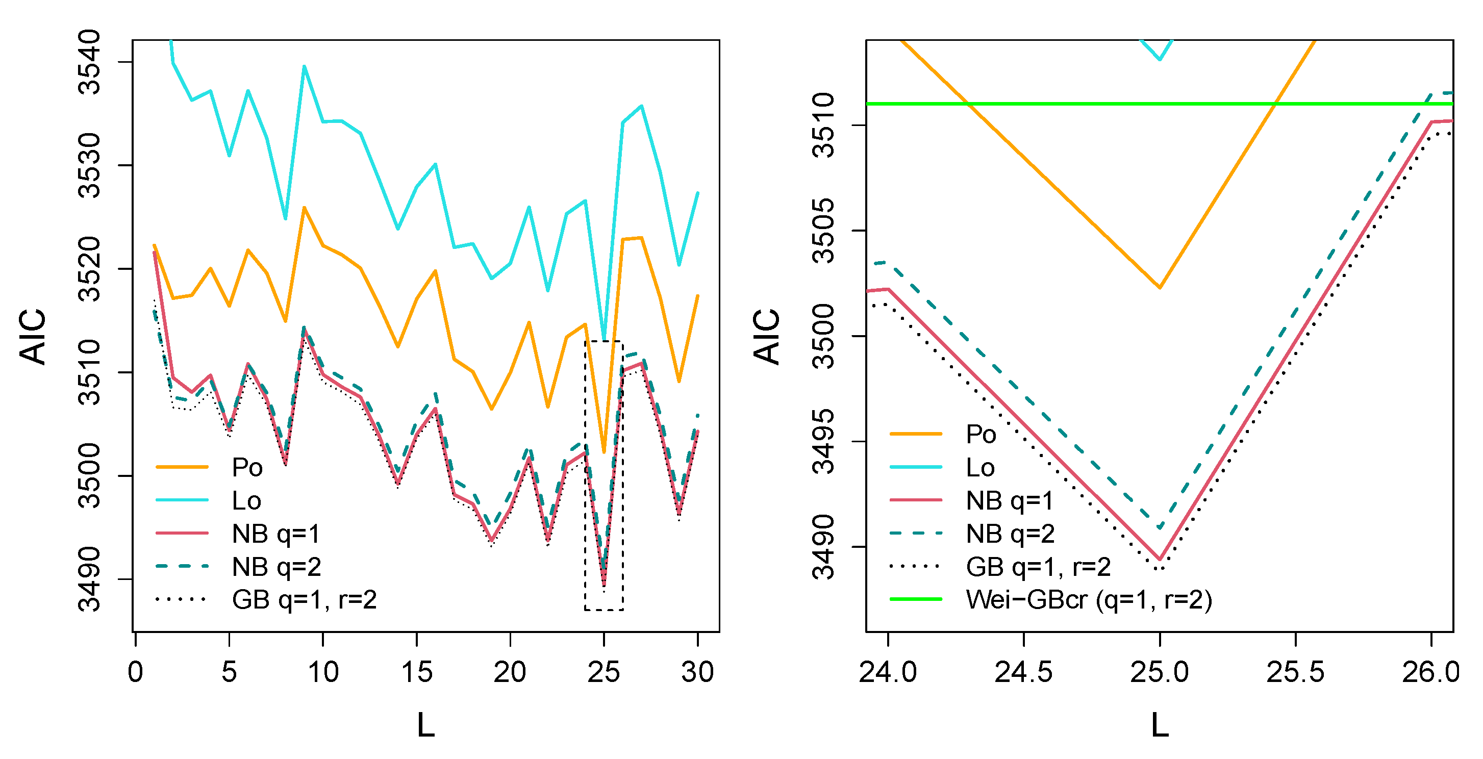
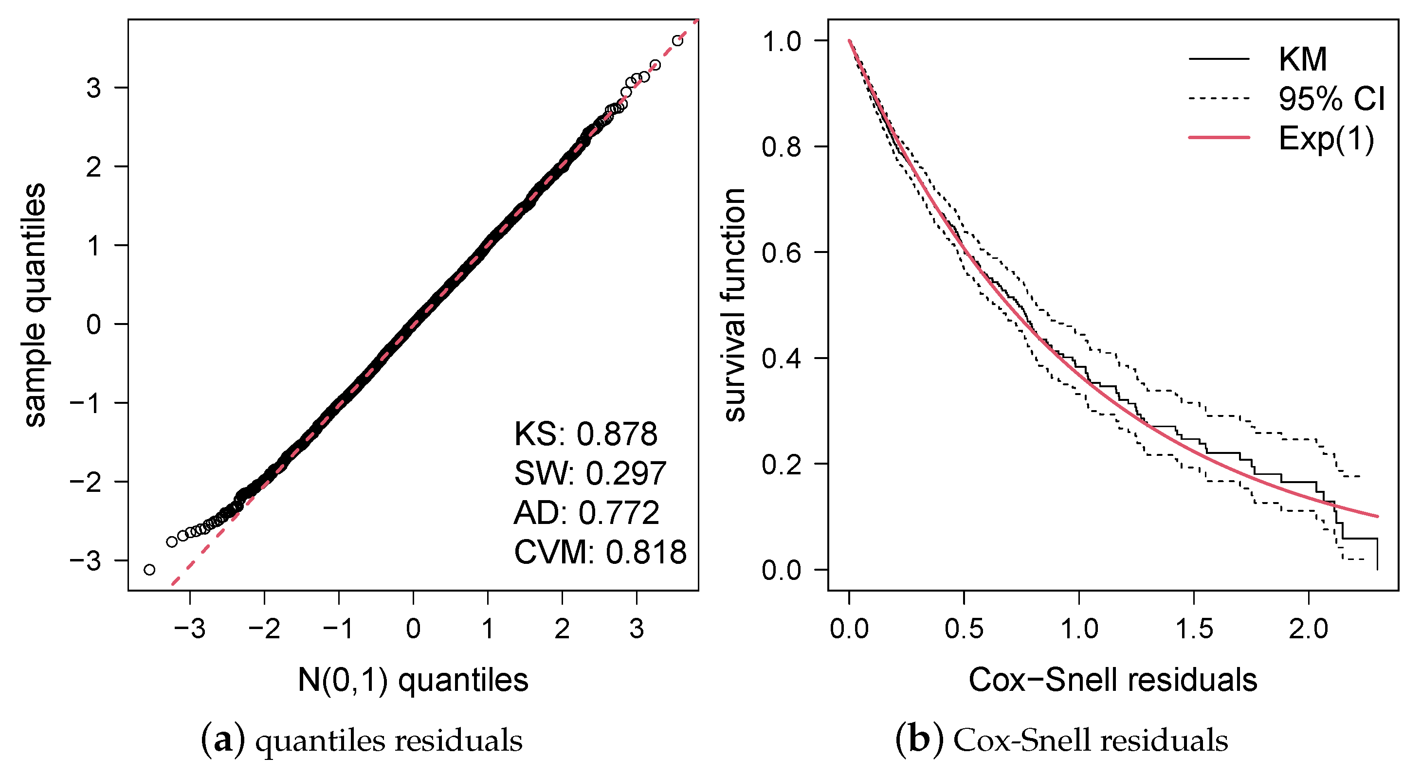
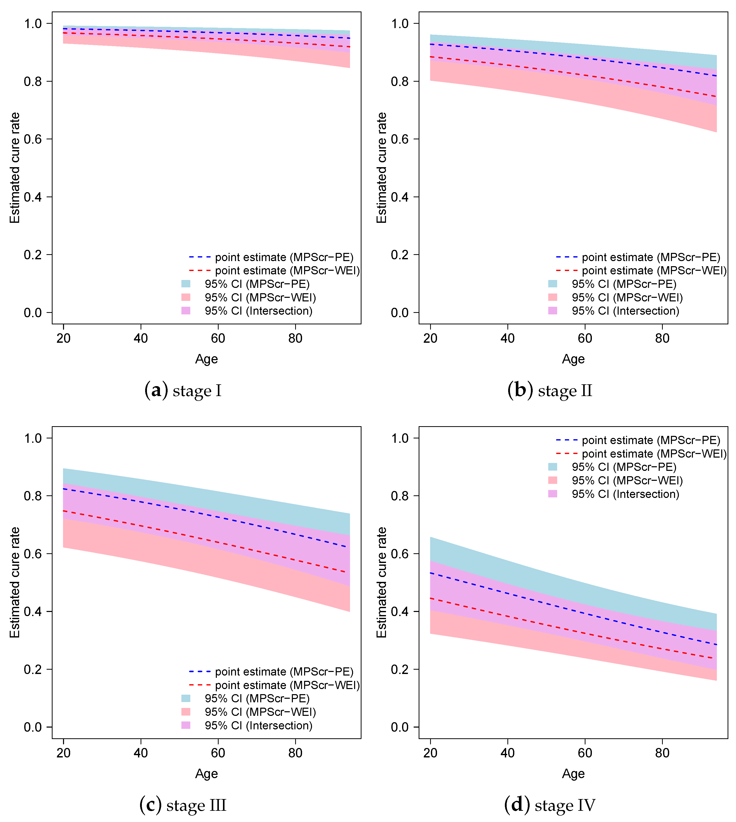
6. Application
7. Conclusions and Future Work
Author Contributions
Funding
Data Availability Statement
Conflicts of Interest
References
- Yin, G.; Ibrahim, J.G. Cure rate models: A unified approach. Can. J. Stat. 2005, 33, 559–570. [Google Scholar] [CrossRef]
- Berkson, J.; Gage, R.P. Survival curve for cancer patients following treatment. J. Am. Stat. Assoc. 1952, 47, 501–515. [Google Scholar] [CrossRef]
- Chen, M.H.; Ibrahim, J.G.; Sinha, D. A new Bayesian model for survival data with a surviving fraction. J. Am. Stat. Assoc. 1999, 94, 909–919. [Google Scholar] [CrossRef]
- Cancho, V.G.; Rodrigues, J.; de Castro, M. A flexible model for survival data with a cure rate: A Bayesian approach. J. Appl. Stat. 2011, 38, 57–70. [Google Scholar] [CrossRef]
- Yiqi, B.; Maria Russo, C.; Cancho, V.G.; Louzada, F. Influence diagnostics for the Weibull-Negative-Binomial regression model with cure rate under latent failure causes. J. Appl. Stat. 2016, 43, 1027–1060. [Google Scholar] [CrossRef]
- Ortega, E.M.; Cordeiro, G.M.; Kattan, M.W. The negative binomial–beta Weibull regression model to predict the cure of prostate cancer. J. Appl. Stat. 2012, 39, 1191–1210. [Google Scholar] [CrossRef]
- D’Andrea, A.; Rocha, R.; Tomazella, V.; Louzada, F. Negative binomial Kumaraswamy-G cure rate regression model. J. Risk Financ. Manag. 2018, 11, 6. [Google Scholar] [CrossRef]
- Gómez, Y.M.; Gallardo, D.I.; Leão, J.; Calsavara, V.F. On a new piecewise regression model with cure rate: Diagnostics and application to medical data. Stat. Med. 2021, 40, 6723–6742. [Google Scholar] [CrossRef] [PubMed]
- de Castro, M.; Gómez, Y.M. A Bayesian cure rate model based on the power piecewise exponential distribution. Methodol. Comput. Appl. Probab. 2020, 22, 677–692. [Google Scholar] [CrossRef]
- Leão, J.; Bourguignon, M.; Gallardo, D.I.; Rocha, R.; Tomazella, V. A new cure rate model with flexible competing causes with applications to melanoma and transplantation data. Stat. Med. 2020, 39, 3272–3284. [Google Scholar] [CrossRef]
- Cancho, V.G.; Louzada, F.; Ortega, E.M. The power series cure rate model: An application to a cutaneous melanoma data. Commun. Stat.-Simul. Comput. 2013, 42, 586–602. [Google Scholar] [CrossRef]
- Balakrishnan, N.; Pal, S. Expectation maximization-based likelihood inference for flexible cure rate models with Weibull lifetimes. Stat. Methods Med. Res. 2016, 25, 1535–1563. [Google Scholar] [CrossRef]
- Balakrishnan, N.; Koutras, M.V.; Milienos, F.S. A weighted Poisson distribution and its application to cure rate models. Commun. Stat.-Theory Methods 2018, 47, 4297–4310. [Google Scholar] [CrossRef]
- Gallardo, D.I.; Gomez, Y.M.; Gómez, H.W.; de Castro, M. On the use of the modified power series family of distributions in a cure rate model context. Stat. Methods Med. Res. 2020, 29, 1831–1845. [Google Scholar] [CrossRef]
- Feigl, P.; Zelen, M. Estimation of exponential survival probabilities with concomitant information. Biometrics 1965, 21, 826–838. [Google Scholar] [CrossRef]
- Friedman, M. Piecewise exponential models for survival data with covariates. Ann. Stat. 1982, 10, 101–113. [Google Scholar] [CrossRef]
- Gómez, Y.M.; Gallardo, D.I.; Arnold, B.C. The power piecewise exponential model. J. Stat. Comput. Simul. 2018, 88, 825–840. [Google Scholar] [CrossRef]
- Gupta, R.D.; Kundu, D. Generalized exponential distributions. Aust. N. Z. J. Stat. 1999, 41, 173–188. [Google Scholar] [CrossRef]
- Dempster, A.P.; Laird, N.M.; Rubin, D.B. Maximum Likelihood from Incomplete Data Via the EM Algorithm. J. R. Stat. Soc. Ser. B (Methodol.) 1977, 39, 1–22. [Google Scholar] [CrossRef]
- Noack, A. A Class of Random Variables with Discrete Distributions. Ann. Math. Stat. 1950, 21, 127–132. [Google Scholar] [CrossRef]
- R Core Team. R: A Language and Environment for Statistical Computing; R Foundation for Statistical Computing: Vienna, Austria, 2023. [Google Scholar]
- Borchers, H.W. pracma: Practical Numerical Math Functions; R Package Version 2.4.2; R Package Vignette: Madison, WI, USA, 2022. [Google Scholar]
- Akaike, H. A new look at the statistical model identification. IEEE Trans. Autom. Control. 1974, 19, 716–723. [Google Scholar] [CrossRef]
- Schwarz, G. Estimating the dimension of a model. Ann. Stat. 1978, 6, 461–464. [Google Scholar] [CrossRef]
- Cox, D.R.; Snell, E.J. A general definition of residuals. J. R. Stat. Soc. Ser. B (Methodol.) 1968, 30, 248–275. [Google Scholar] [CrossRef]
- Kolmogorov, A.N. Sulla determinazione empirica di una legge di distribuzione (On the empirical determination of a distribution law). G. Dell’Inst. Ital. Degli Attuari 1933, 4, 83–91. [Google Scholar]
- Shapiro, S.S.; Wilk, M.B. An analysis of variance test for normality (complete samples). Biometrika 1965, 52, 591–611. [Google Scholar] [CrossRef]
- Anderson, T.W.; Darling, D.A. Asymptotic theory of certain “goodness of fit” criteria based on stochastic processes. Ann. Math. Stat. 1952, 23, 193–212. [Google Scholar] [CrossRef]
- Cramér, H. On the composition of elementary errors. Skand. Aktuarietidskr. 1928, 11, 13–74. [Google Scholar]


| Distribution | |||||
|---|---|---|---|---|---|
| Bin | |||||
| Po | |||||
| NB | |||||
| Lo | |||||
| Bo | |||||
| Ha | |||||
| GB | |||||
| RGP |
| Cens. | Parameter | Bias | RMSE | SE | Bias | RMSE | SE | Bias | RMSE | SE | |
|---|---|---|---|---|---|---|---|---|---|---|---|
| 10 | 1.526 | 2.103 | 3.269 | 1.404 | 1.607 | 0.803 | 1.375 | 1.466 | 0.523 | ||
| −0.259 | 1.398 | 3.065 | −0.147 | 0.693 | 0.634 | −0.108 | 0.390 | 0.375 | |||
| −0.41 | 1.429 | 3.048 | −0.282 | 0.729 | 0.621 | −0.253 | 0.450 | 0.364 | |||
| 2.848 | 3.655 | 9.754 | 2.753 | 2.934 | 1.437 | 2.749 | 2.825 | 0.738 | |||
| 0.002 | 0.009 | 0.009 | 0.001 | 0.007 | 0.007 | 0.001 | 0.006 | 0.006 | |||
| −0.136 | 0.178 | 0.115 | −0.149 | 0.174 | 0.091 | −0.152 | 0.171 | 0.078 | |||
| 0.081 | 0.091 | 0.045 | 0.076 | 0.083 | 0.036 | 0.076 | 0.082 | 0.031 | |||
| 0.097 | 0.105 | 0.042 | 0.097 | 0.103 | 0.034 | 0.094 | 0.098 | 0.029 | |||
| 0.264 | 0.269 | 0.080 | 0.260 | 0.264 | 0.064 | 0.258 | 0.261 | 0.055 | |||
| 1 | 1.709 | 2.186 | 2.537 | 1.634 | 1.874 | 1.203 | 1.573 | 1.660 | 0.562 | ||
| −0.262 | 1.321 | 2.324 | −0.202 | 0.835 | 1.031 | −0.158 | 0.460 | 0.412 | |||
| -0.468 | 1.375 | 2.305 | −0.403 | 0.891 | 1.015 | −0.351 | 0.545 | 0.399 | |||
| 2.964 | 3.948 | 13.983 | 2.721 | 3.028 | 2.670 | 2.752 | 2.849 | 0.841 | |||
| 0.001 | 0.009 | 0.010 | 0.001 | 0.007 | 0.008 | 0.001 | 0.006 | 0.007 | |||
| −0.114 | 0.227 | 0.186 | −0.130 | 0.192 | 0.148 | −0.133 | 0.184 | 0.127 | |||
| 0.091 | 0.104 | 0.053 | 0.086 | 0.095 | 0.042 | 0.084 | 0.090 | 0.036 | |||
| 0.100 | 0.108 | 0.043 | 0.100 | 0.106 | 0.035 | 0.099 | 0.104 | 0.030 | |||
| 0.268 | 0.273 | 0.076 | 0.266 | 0.269 | 0.061 | 0.266 | 0.268 | 0.053 | |||
| 2.226 | 3.217 | 7.454 | 1.945 | 2.431 | 2.326 | 1.797 | 1.920 | 0.733 | |||
| −0.623 | 2.380 | 7.245 | −0.333 | 1.414 | 2.153 | −0.220 | 0.637 | 0.580 | |||
| −0.894 | 2.451 | 7.223 | −0.607 | 1.487 | 2.134 | −0.471 | 0.744 | 0.565 | |||
| 2.976 | 4.876 | 29.816 | 2.818 | 3.579 | 7.902 | 2.754 | 2.990 | 2.057 | |||
| 0.001 | 0.009 | 0.010 | 0.001 | 0.008 | 0.008 | 0.001 | 0.007 | 0.007 | |||
| −0.039 | 0.353 | 0.299 | −0.082 | 0.255 | 0.229 | −0.095 | 0.209 | 0.195 | |||
| 0.104 | 0.123 | 0.063 | 0.099 | 0.110 | 0.051 | 0.095 | 0.103 | 0.043 | |||
| 0.105 | 0.114 | 0.045 | 0.105 | 0.111 | 0.037 | 0.106 | 0.110 | 0.032 | |||
| 0.277 | 0.282 | 0.075 | 0.272 | 0.275 | 0.060 | 0.271 | 0.273 | 0.052 | |||
| 14 | 1.191 | 1.519 | 1.283 | 1.098 | 1.221 | 0.556 | 1.123 | 1.216 | 0.479 | ||
| −0.128 | 0.842 | 1.083 | −0.074 | 0.387 | 0.391 | −0.067 | 0.344 | 0.336 | |||
| −0.195 | 0.854 | 1.070 | −0.136 | 0.390 | 0.380 | −0.135 | 0.356 | 0.327 | |||
| 2.859 | 3.314 | 4.944 | 2.796 | 2.878 | 0.921 | 2.753 | 2.793 | 0.474 | |||
| 0.002 | 0.009 | 0.009 | 0.002 | 0.007 | 0.007 | 0.002 | 0.006 | 0.006 | |||
| −0.133 | 0.173 | 0.111 | −0.141 | 0.165 | 0.090 | −0.146 | 0.163 | 0.077 | |||
| 0.055 | 0.064 | 0.036 | 0.053 | 0.059 | 0.029 | 0.052 | 0.057 | 0.025 | |||
| 0.059 | 0.067 | 0.031 | 0.059 | 0.064 | 0.026 | 0.058 | 0.062 | 0.022 | |||
| 0.140 | 0.144 | 0.044 | 0.139 | 0.142 | 0.036 | 0.141 | 0.143 | 0.031 | |||
| 1 | 1.366 | 1.791 | 1.889 | 1.269 | 1.391 | 0.583 | 1.238 | 1.327 | 0.501 | ||
| −0.194 | 1.110 | 1.688 | −0.098 | 0.439 | 0.417 | −0.076 | 0.360 | 0.355 | |||
| −0.309 | 1.117 | 1.672 | −0.207 | 0.466 | 0.405 | −0.178 | 0.386 | 0.345 | |||
| 2.888 | 3.605 | 8.757 | 2.792 | 2.888 | 0.959 | 2.776 | 2.824 | 0.505 | |||
| 0.002 | 0.008 | 0.009 | 0.001 | 0.007 | 0.007 | 0.002 | 0.006 | 0.006 | |||
| −0.107 | 0.222 | 0.179 | −0.133 | 0.190 | 0.140 | −0.127 | 0.174 | 0.122 | |||
| 0.064 | 0.077 | 0.042 | 0.061 | 0.068 | 0.034 | 0.062 | 0.067 | 0.030 | |||
| 0.063 | 0.071 | 0.032 | 0.062 | 0.067 | 0.026 | 0.062 | 0.065 | 0.023 | |||
| 0.146 | 0.149 | 0.042 | 0.144 | 0.146 | 0.034 | 0.144 | 0.146 | 0.029 | |||
| 1.688 | 2.495 | 4.575 | 1.413 | 1.547 | 0.618 | 1.406 | 1.504 | 0.531 | |||
| −0.420 | 1.847 | 4.375 | −0.146 | 0.498 | 0.449 | −0.131 | 0.438 | 0.384 | |||
| −0.563 | 1.877 | 4.358 | −0.286 | 0.545 | 0.436 | −0.274 | 0.485 | 0.373 | |||
| 2.731 | 3.766 | 12.322 | 2.767 | 2.954 | 1.973 | 2.700 | 2.790 | 0.745 | |||
| 0.001 | 0.009 | 0.009 | 0.001 | 0.007 | 0.007 | 0.001 | 0.006 | 0.006 | |||
| −0.014 | 0.336 | 0.290 | −0.047 | 0.254 | 0.226 | −0.072 | 0.206 | 0.189 | |||
| 0.081 | 0.097 | 0.053 | 0.076 | 0.086 | 0.043 | 0.072 | 0.080 | 0.036 | |||
| 0.068 | 0.076 | 0.035 | 0.068 | 0.073 | 0.028 | 0.068 | 0.071 | 0.024 | |||
| 0.154 | 0.156 | 0.041 | 0.153 | 0.155 | 0.033 | 0.152 | 0.153 | 0.029 | |||
| Cens. | Parameter | Bias | RMSE | SE | Bias | RMSE | SE | Bias | RMSE | SE | |
|---|---|---|---|---|---|---|---|---|---|---|---|
| 18 | 1.024 | 1.313 | 1.168 | 0.968 | 1.083 | 0.525 | 0.971 | 1.067 | 0.454 | ||
| −0.089 | 0.704 | 0.972 | −0.021 | 0.363 | 0.363 | −0.031 | 0.324 | 0.315 | |||
| −0.118 | 0.701 | 0.96 | −0.046 | 0.341 | 0.354 | −0.056 | 0.324 | 0.307 | |||
| 2.753 | 2.931 | 1.679 | 2.803 | 2.848 | 0.519 | 2.760 | 2.796 | 0.444 | |||
| 0.002 | 0.008 | 0.008 | 0.002 | 0.006 | 0.007 | 0.002 | 0.006 | 0.006 | |||
| −0.136 | 0.176 | 0.109 | −0.143 | 0.166 | 0.088 | −0.146 | 0.162 | 0.076 | |||
| 0.042 | 0.052 | 0.031 | 0.040 | 0.047 | 0.025 | 0.040 | 0.045 | 0.022 | |||
| 0.042 | 0.049 | 0.027 | 0.041 | 0.046 | 0.021 | 0.041 | 0.044 | 0.019 | |||
| 0.092 | 0.095 | 0.031 | 0.092 | 0.094 | 0.025 | 0.091 | 0.092 | 0.022 | |||
| 1 | 1.108 | 1.366 | 0.975 | 1.086 | 1.312 | 0.727 | 1.042 | 1.132 | 0.468 | ||
| −0.096 | 0.680 | 0.776 | −0.078 | 0.648 | 0.564 | −0.026 | 0.328 | 0.325 | |||
| −0.147 | 0.674 | 0.763 | −0.131 | 0.650 | 0.554 | −0.080 | 0.327 | 0.316 | |||
| 2.791 | 3.011 | 1.857 | 2.763 | 2.863 | 0.728 | 2.771 | 2.808 | 0.461 | |||
| 0.002 | 0.008 | 0.008 | 0.002 | 0.007 | 0.007 | 0.002 | 0.006 | 0.006 | |||
| −0.111 | 0.206 | 0.174 | −0.125 | 0.186 | 0.138 | −0.127 | 0.173 | 0.119 | |||
| 0.051 | 0.062 | 0.037 | 0.049 | 0.056 | 0.030 | 0.048 | 0.054 | 0.026 | |||
| 0.045 | 0.052 | 0.027 | 0.046 | 0.050 | 0.022 | 0.046 | 0.049 | 0.019 | |||
| 0.097 | 0.099 | 0.030 | 0.095 | 0.096 | 0.024 | 0.095 | 0.097 | 0.021 | |||
| 1.278 | 1.760 | 1.98 | 1.157 | 1.276 | 0.564 | 1.151 | 1.244 | 0.485 | |||
| −0.154 | 1.136 | 1.777 | −0.065 | 0.415 | 0.398 | −0.082 | 0.360 | 0.343 | |||
| −0.231 | 1.146 | 1.763 | −0.139 | 0.423 | 0.386 | −0.147 | 0.376 | 0.333 | |||
| 2.778 | 3.181 | 3.230 | 2.775 | 2.834 | 0.567 | 2.728 | 2.772 | 0.480 | |||
| 0.001 | 0.008 | 0.009 | 0.002 | 0.007 | 0.007 | 0.002 | 0.006 | 0.006 | |||
| −0.021 | 0.330 | 0.279 | −0.054 | 0.220 | 0.215 | −0.068 | 0.200 | 0.183 | |||
| 0.066 | 0.081 | 0.047 | 0.062 | 0.070 | 0.037 | 0.060 | 0.067 | 0.032 | |||
| 0.051 | 0.058 | 0.030 | 0.049 | 0.054 | 0.024 | 0.048 | 0.052 | 0.020 | |||
| 0.100 | 0.103 | 0.029 | 0.099 | 0.100 | 0.023 | 0.100 | 0.101 | 0.020 | |||
| Distribution | PPE | Weibull | ||||
|---|---|---|---|---|---|---|
| Cure Rate Model | Loglike | AIC | BIC | Loglike | AIC | BIC |
| Pocr | −1720.2 | 3502.4 | 3526.7 | −1752.3 | 3518.7 | 3591.0 |
| Locr | −1725.6 | 3513.2 | 3537.6 | −1766.1 | 3546.2 | 3618.6 |
| NBcr | −1713.7 | 3489.4 | 3513.7 | −1751.6 | 3517.3 | 3589.6 |
| NBcr | −1714.5 | 3490.9 | 3515.2 | −1749.5 | 3512.9 | 3585.3 |
| GBcr | −1713.4 | 3488.8 | 3513.1 | −1748.5 | 3511.0 | 3583.3 |
| GBcr-PE and | |||||||
| GBcr-WEI and | |||||||
Disclaimer/Publisher’s Note: The statements, opinions and data contained in all publications are solely those of the individual author(s) and contributor(s) and not of MDPI and/or the editor(s). MDPI and/or the editor(s) disclaim responsibility for any injury to people or property resulting from any ideas, methods, instructions or products referred to in the content. |
© 2024 by the authors. Licensee MDPI, Basel, Switzerland. This article is an open access article distributed under the terms and conditions of the Creative Commons Attribution (CC BY) license (https://creativecommons.org/licenses/by/4.0/).
Share and Cite
Gómez, Y.M.; Santibañez, J.L.; Calsavara, V.F.; Gómez, H.W.; Gallardo, D.I. A Modified Cure Rate Model Based on a Piecewise Distribution with Application to Lobular Carcinoma Data. Mathematics 2024, 12, 883. https://doi.org/10.3390/math12060883
Gómez YM, Santibañez JL, Calsavara VF, Gómez HW, Gallardo DI. A Modified Cure Rate Model Based on a Piecewise Distribution with Application to Lobular Carcinoma Data. Mathematics. 2024; 12(6):883. https://doi.org/10.3390/math12060883
Chicago/Turabian StyleGómez, Yolanda M., John L. Santibañez, Vinicius F. Calsavara, Héctor W. Gómez, and Diego I. Gallardo. 2024. "A Modified Cure Rate Model Based on a Piecewise Distribution with Application to Lobular Carcinoma Data" Mathematics 12, no. 6: 883. https://doi.org/10.3390/math12060883
APA StyleGómez, Y. M., Santibañez, J. L., Calsavara, V. F., Gómez, H. W., & Gallardo, D. I. (2024). A Modified Cure Rate Model Based on a Piecewise Distribution with Application to Lobular Carcinoma Data. Mathematics, 12(6), 883. https://doi.org/10.3390/math12060883