On Self-Intersections of Cubic Bézier Curves

Abstract

Cubic Bézier curves are widely used in computer graphics and geometric modeling, favored for their intuitive design and ease of implementation. However, self-intersections within these curves can pose significant challenges in both geometric modeling and analysis. This paper presents a comprehensive approach to detecting and computing self-intersections of cubic Bézier curves. We introduce an efficient algorithm that leverages both the geometric properties of Bézier curves and numerical methods to accurately identify intersection points. The self-intersection problem of cubic Bézier curves is firstly transformed into a quadratic problem by eliminating trivial solutions. Subsequently, this quadratic system is converted into a linear system that may be easily analyzed and solved. Finally, the parameter values corresponding to the self-intersection points are computed through the solution of the linear system. The proposed method is designed to be robust and computationally efficient, making it suitable for real-time applications.

1. Introduction

The representation of free-form curves and surfaces is a foundational research topic within Computer-Aided Geometric Design (CAGD) and computer graphics (CG), as well as various related fields [1]. Bézier curves and surfaces, constructed through control points and Bernstein basis functions, represent one of the most pivotal methodologies in this domain. Owing to the intrinsic properties of Bernstein basis functions, Bézier entities exhibit several advantageous characteristics, such as affine invariance, the convex hull property, and endpoint interpolation. The manipulation of control points allows for nuanced and intuitive shape control of Bézier curves and surfaces, facilitating their widespread application.

The identification of self-intersections in free-form curves and surfaces is a critical requirement across various Computer-Aided Design (CAD) and Computer-Aided Manufacturing (CAM) applications, such as NC machining and robotic navigation [2]. For example, during the process of image deformation, self-intersection in the parameterization can cause image overlapping, distortion, and loss of information. In addition, surfaces with self-intersecting cross-section curves are difficult to manufacture directly using CNC machines in the field of mechanical engineering. Recognizing this, Hoffman has highlighted the self-intersection computation of parametric curves and surfaces as one of the most fundamental issues in geometric and solid modeling [3,4].

Given the importance of this issue, numerous researchers have dedicated their efforts to identifying and efficiently calculating self-intersection points in free-form curves and surfaces. Techniques such as light and shadow tracing have been employed to compute these self-intersections, though they may not always yield accurate results. Barnhill et al. [5] introduced a marching method that initially identifies potential intersection branches, a process that, however, is susceptible to generating phantom branches and thus may produce erroneous outcomes. Su and Liu [6] explored curve singularities (self-intersections, cusps) and inflection points using the affine-invariant method (AIM), revealing that the characteristic points of a curve align with its characteristic distribution graph in the presence of self-intersections. Building on this concept, Ye [7] developed a simpler method to map the distribution of singularities and inflection points, enabling the identification of characteristic point regions in planar cubic Bézier curves without resorting to solving equations. This methodology has inspired subsequent studies on the distribution of singularities in specific curve types, such as C-Bézier and F-Bézier curves [8,9,10,11]. Lasser [12] introduced a curve–curve method that evaluates the cumulative rotation angle of the tangent vector to detect and calculate self-intersections in Bézier curves. However, the lack of a theoretical proof within this method may affect the reliability of its predictions in some scenarios. Further advancements by Zhu and Zhao [13,14] provided sufficient and necessary conditions for rational Bézier curves and surfaces to be self-intersection-free, employing toric degeneration theory and well-posedness conditions. Yet the stringent bijectivity conditions set forth in these studies are often too restrictive, leading to inaccuracies when determining the bijectivity of Bézier curves in practical situations. Yu et al. [15,16] introduced algorithms to assess self-intersections in toric surfaces and volumes, applicable to Bézier geometries. For more information on self-intersection studies in curves and surfaces, interested readers can refer to [17,18,19].

In practical scenarios, quadratic and cubic Bézier curves are favored for their robust capability in geometric representation, along with their cost-effective computational costs and numerical stability, as compared to their higher-degree counterparts. Yet the current algorithms for identifying self-intersections do not cater specifically to cubic Bézier curves, which leads to computational inefficiencies in these instances. Furthermore, the bijectivity conditions proposed in [12,13] may prove overly stringent for a range of practical applications.

This paper proposes a simple yet effective method for computing all self-intersections of cubic Bézier curves. Drawing on the algebraic decomposition approach as discussed in [20,21], the self-intersection problem of cubic Bézier curves can be firstly transformed into a quadratic problem by eliminating the trivial solutions. Subsequently, this quadratic system is converted into a linear system that may be easily analysed and solved. Finally, the parameter values corresponding to the self-intersection points are obtained through the solution of the aforementioned linear system. The proposed methodology offers an efficient and precise computation of all self-intersections within cubic Bézier curves, overcoming the limitations of the existing algorithms as noted in [12,13].

The remainder of this paper is structured as follows. Section 2 details the methodology for computing self-intersections in cubic Bézier curves. Section 3 showcases numerical experiments to demonstrate the effectiveness and efficiency of the proposed method. Finally, Section 4 summarizes our findings and contributions.

2. Methodology

In this section, we discuss both the existence and the fast computation of self-intersections in cubic Bézier curves. Section 2.1 provides a brief introduction to cubic Bernstein basis functions and cubic Bézier curves. Section 2.2 discusses the scenario where the four control points of the cubic Bézier curve are collinear, while Section 2.3 covers the case in which they are not collinear.

2.1. Cubic Bernstein Basis Functions and Bézier Curves

Bernstein basis functions are polynomials that have a partition of unity and are non-negative over the interval $[0,1]$. Bernstein basis functions of degree n are expressed as

$$B_i^n\left(\xi \right)=\left(\genfrac{}{}{0pt}{}{n}{i}\right){(1-\xi )}^{n-i}{\xi }^i,\xi \in [0,1],$$

(1)

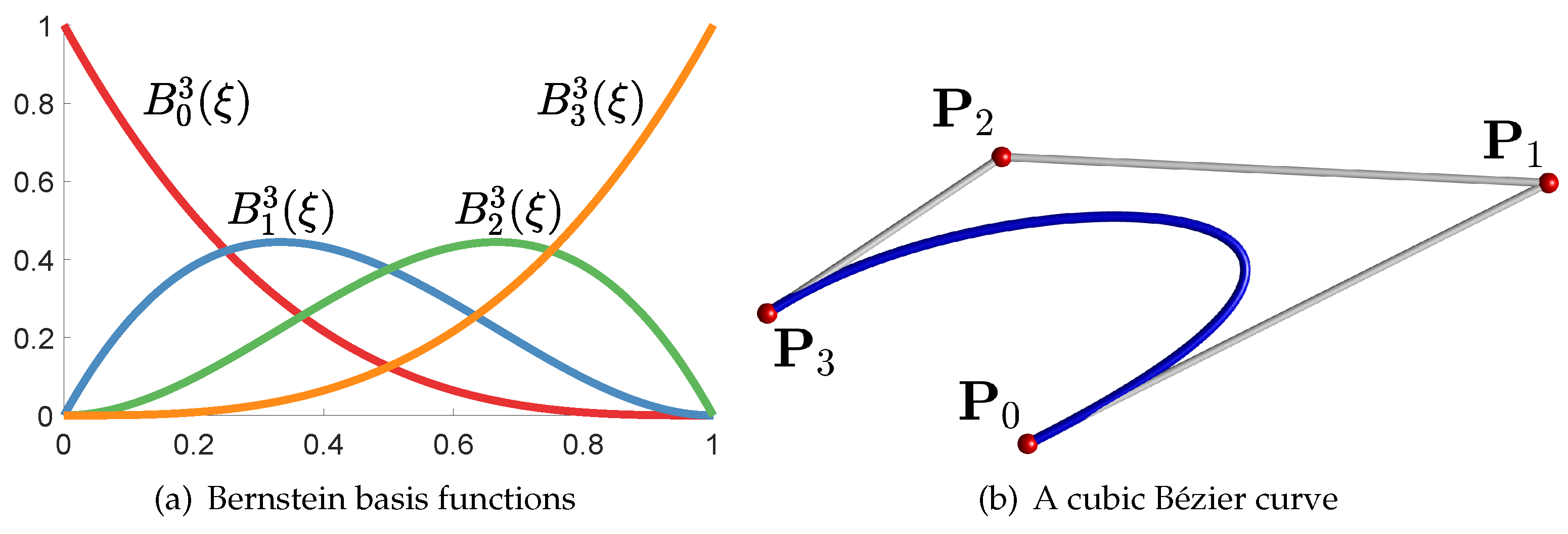
for $i=0,1,\dots ,n$. Figure 1a illustrates cubic Bernstein basis functions with $n=3$.

The Bernstein basis functions (1) form the mathematical foundation of Bézier curves, a class of parametric curves extensively used in computer graphics, animation, and CAD systems due to their intuitive design and easy computation. A cubic Bézier curve is defined as a linear combination of four control points ${\mathbf{P}}_i={(x_i,y_i,z_i)}^{\mathrm{T}}\in {\mathbb{R}}^3$ ($i=0,1,2,3$), with the degree-3 Bernstein basis functions as coefficients. Then, a cubic Bézier curve is defined as the image of the following vector-valued parametric function [1]

$$\mathcal{C}\left(\xi \right)=\left(\begin{array}{c}x\left(\xi \right)\\ y\left(\xi \right)\\ z\left(\xi \right)\end{array}\right)=\left(\begin{array}{c}\sum _{i=0}^3{x}_i{B}_i^3\left(\xi \right)\\ \sum _{i=0}^3{y}_i{B}_i^3\left(\xi \right)\\ \sum _{i=0}^3{z}_i{B}_i^3\left(\xi \right)\end{array}\right)=\sum _{i=0}^3{\mathbf{P}}_i{B}_i^3\left(\xi \right),\xi \in [0,1].$$

(2)

Figure 1b illustrates a cubic Bézier curve. Due to the specific properties of Bernstein polynomials, such as the fact that the sum of their values at any given $\xi$ is always one, the resulting Bézier curve exhibits strong stability and predictable behavior, making it a preferred tool for curve design. The partition of unity and non-negativity property of Bernstein basis functions ensures that the curve lies within the convex hull of its control points ${\mathbf{P}}_i$ ($i=0,1,2,3$). In addition, Bézier curves possess the affine invariance property, meaning that their shape is preserved under affine transformations, providing a useful property for various geometric modeling applications and computations.

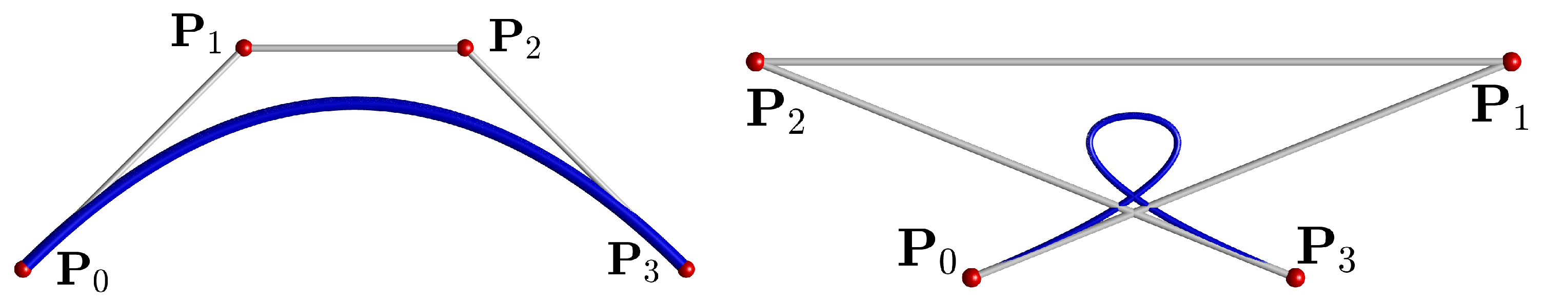
Self-intersections in cubic Bézier curves are of significant interest due to their implications in design and rendering processes. A cubic Bézier curve may intersect itself depending on the geometric configuration of its control points when there are distinct parameters ${\xi }_1$ and ${\xi }_2$ such that $\mathcal{C}\left({\xi }_1\right)=\mathcal{C}\left({\xi }_2\right)$. Figure 2a shows a cubic Bézier curve that is free of self-intersections, while Figure 2b presents a cubic Bézier curve that intersects itself due to the placement of specific control points. Both serve as examples for understanding the geometric implications of control point configurations in curve design.

2.2. Cubic Bézier Curves with Collinear Control Points

Consider the four control points ${\left\{{\mathbf{P}}_i\right\}}_{i=0}^3$ of a cubic Bézier curve $\mathcal{C}\left(\xi \right)$ to be collinear, i.e., satisfying $\overrightarrow{{\mathbf{P}}_0{\mathbf{P}}_j}=k_j\overrightarrow{{\mathbf{P}}_0{\mathbf{P}}_3}$$(j=1,2)$. Thanks to the affine invariance property of Bézier curves, its shape remains unaltered by translation and rotation transformations. Therefore, we apply Rodrigues’ rotation formula to translate and rotate the control points ${\left\{{\mathbf{P}}_i\right\}}_{i=0}^3$ to ${\left\{{\tilde{\mathbf{P}}}_i\right\}}_{i=0}^3$, positioning ${\tilde{\mathbf{P}}}_0$ at the origin ${(0,0,0)}^{\mathrm{T}}$ and aligning ${\tilde{\mathbf{P}}}_3$ along the positive x-axis at a distance ${\tilde{x}}_3=\sqrt{{(x_3-x_0)}^2+{(y_3-y_0)}^2+{(z_3-z_0)}^2}$, i.e., ${\tilde{\mathbf{P}}}_3={({\tilde{x}}_3,0,0)}^{\mathrm{T}}$. This adjustment sets the x-coordinate of ${\left\{{\tilde{\mathbf{P}}}_j\right\}}_{j=1,2}$ to $k_j{\tilde{x}}_3$. Under these transformations, the cubic Bézier curve $\tilde{\mathcal{C}}\left(\xi \right)$, redefined by the control points ${\left\{{\tilde{\mathbf{P}}}_i\right\}}_{i=0}^3$, simplifies to a linear trajectory along the x-axis, and can be expressed as

$$\tilde{\mathcal{C}}\left(\xi \right)=\left[(3k_1-3k_2+1){\tilde{x}}_3\right]{\xi }^3+\left[(3k_2-6k_1){\tilde{x}}_3\right]{\xi }^2+3k_1{\tilde{x}}_3\xi .$$

(3)

To analyze the trend of the cubic Bézier curve $\tilde{\mathcal{C}}\left(\xi \right)$, we examine its derivative as derived from Equation (3)

$${\tilde{\mathcal{C}}}^{\prime }\left(\xi \right)=3\left[(3k_1-3k_2+1){\tilde{x}}_3\right]{\xi }^2+2\left[(3k_2-6k_1){\tilde{x}}_3\right]\xi +3k_1{\tilde{x}}_3.$$

(4)

The monotonicity of $\tilde{\mathcal{C}}\left(\xi \right)$ hinges on the solvability of its derivative function ${\tilde{\mathcal{C}}}^{\prime }\left(\xi \right)$. Concurrently, the presence of solutions for the derivative function, as defined in Equation (4), is contingent upon the value of its discriminant

$$\begin{array}{cc}\hfill \tilde{\Delta }& ={\left(2\left[(3k_2-6k_1){\tilde{x}}_3\right]\right)}^2-4\times 3\left[(3k_1-3k_2+1){\tilde{x}}_3\right]\times 3k_1{\tilde{x}}_3\hfill \\ \hfill & =36{\tilde{x}}_3^2(k_1^2+k_2^2-k_1{k}_2-k_1).\hfill \end{array}$$

(5)

Based on the calculations in (3)–(5), we are now prepared to articulate the following theorem.

Theorem 1.

Consider the set of control points ${\left\{{\mathbf{P}}_i\right\}}_{i=0}^3$ lying on a straight line, fulfilling the condition $\overrightarrow{{\mathbf{P}}_0{\mathbf{P}}_j}=k_j\overrightarrow{{\mathbf{P}}_0{\mathbf{P}}_3}$$(j=1,2)$, for a cubic Bézier curve $\mathcal{C}\left(\xi \right)$. The cubic Bézier curve $\mathcal{C}\left(\xi \right)$ is self-overlapping if and only if $k_1^2+k_2^2-k_1{k}_2-k_1>0$ holds; otherwise it has no self-intersections.

Proof. 

Upon applying translation and rotation to the curve $\tilde{\mathcal{C}}\left(\xi \right)$ as defined in Equation (3), a condition arises where $k_1^2+k_2^2-k_1{k}_2-k_1>0$ leads to a consistently positive discriminant in Equation (5). Under these circumstances, the quadratic derivative function ${\tilde{\mathcal{C}}}^{\prime }\left(\xi \right)$ in Equation (4) possesses two distinct roots, indicating a change in the monotonicity of the cubic function $\tilde{\mathcal{C}}\left(\xi \right)$ at these roots. Given that the control points are aligned collinearly, the cubic Bézier curve $\tilde{\mathcal{C}}\left(\xi \right)$ is constrained to the line defined by these points and maintains continuity. A change in monotonicity thus signifies self-overlapping within the curve. In contrast, the absence of such a change denotes a monotonic $\tilde{\mathcal{C}}\left(\xi \right)$ devoid of self-intersections.

According to the affine invariance property of Bézier curves, it follows that $\mathcal{C}\left(\xi \right)$ retains the identical geometric relationships as $\tilde{\mathcal{C}}\left(\xi \right)$.    □

Theorem 1 serves as a pivotal tool for identifying the presence of a self-intersection, or more precisely, a self-overlap in cubic Bézier curves when their control points are aligned collinearly. In the following subsection, our discussion will expand into scenarios where cubic Bézier curves exhibit non-collinear control points.

2.3. Cubic Bézier Curves with Non-Collinear Control Points

Consider the four non-collinear control points ${\mathbf{P}}_i={(x_i,y_i,z_i)}^{\mathrm{T}}$, for $i=0,1,2,3$, of a cubic Bézier curve $\mathcal{C}\left(\xi \right)$. The problem of identifying self-intersections within this curve boils down to determining the parameters ${\xi }_1$ and ${\xi }_2$ such that ${\xi }_1\ne {\xi }_2$ while simultaneously ensuring $\mathcal{C}\left({\xi }_1\right)=\mathcal{C}\left({\xi }_2\right)$. From the definition in Equation (2), that is,

$$\left\{\begin{array}{c}x\left({\xi }_1\right)=x\left({\xi }_2\right)\\ y\left({\xi }_1\right)=y\left({\xi }_2\right)\\ z\left({\xi }_1\right)=z\left({\xi }_2\right)\end{array}\right..$$

(6)

To streamline our analysis, similarly, we reposition the control points ${\left\{{\mathbf{P}}_i\right\}}_{i=0}^3$ to ${\left\{{\widehat{\mathbf{P}}}_i\right\}}_{i=0}^3$, where ${\widehat{\mathbf{P}}}_i={({\widehat{x}}_i,{\widehat{y}}_i,{\widehat{z}}_i)}^{\mathrm{T}}$ and set ${\widehat{\mathbf{P}}}_0$ as the origin. The resulting cubic Bézier curve, represented by the control points ${\left\{{\widehat{\mathbf{P}}}_i\right\}}_{i=0}^3$ and denoted as $\widehat{\mathcal{C}}\left(\xi \right)$, retains identical geometric properties to $\mathcal{C}\left(\xi \right)$.

Substituting the control points ${\left\{{\widehat{\mathbf{P}}}_i\right\}}_{i=0}^3$ and the cubic Bernstein basis functions ${\left\{B_i^3\right\}}_{i=0}^3$ into Equation (6), we have

$$\left\{\begin{array}{c}3{\widehat{x}}_1{\xi }_1{(1-{\xi }_1)}^2+3{\widehat{x}}_2{\xi }_1^2(1-{\xi }_1)+{\widehat{x}}_3{\xi }_1^3=3{\widehat{x}}_1{\xi }_2{(1-{\xi }_2)}^2+3{\widehat{x}}_2{\xi }_2^2(1-{\xi }_2)+{\widehat{x}}_3{\xi }_2^3\hfill \\ 3{\widehat{y}}_1{\xi }_1{(1-{\xi }_1)}^2+3{\widehat{y}}_2{\xi }_1^2(1-{\xi }_1)+{\widehat{y}}_3{\xi }_1^3=3{\widehat{y}}_1{\xi }_2{(1-{\xi }_2)}^2+3{\widehat{y}}_2{\xi }_2^2(1-{\xi }_2)+{\widehat{y}}_3{\xi }_2^3\hfill \\ 3{\widehat{z}}_1{\xi }_1{(1-{\xi }_1)}^2+3{\widehat{z}}_2{\xi }_1^2(1-{\xi }_1)+{\widehat{z}}_3{\xi }_1^3=3{\widehat{z}}_1{\xi }_2{(1-{\xi }_2)}^2+3{\widehat{z}}_2{\xi }_2^2(1-{\xi }_2)+{\widehat{z}}_3{\xi }_2^3\hfill \end{array}\right..$$

(7)

To discuss the solutions of the system (7), we first organize the cubic Bernstein basis functions ${\left\{B_i^3\right\}}_{i=0}^3$ as follows:

$$\begin{array}{cc}\hfill {(1-{\xi }_1)}^3-{(1-{\xi }_2)}^3& =({\xi }_2-{\xi }_1)[3-3({\xi }_1+{\xi }_2)+({\xi }_1^2+{\xi }_1{\xi }_2+{\xi }_2^2)],\hfill \\ \hfill {\xi }_1{(1-{\xi }_1)}^2-{\xi }_2{(1-{\xi }_2)}^2& =({\xi }_2-{\xi }_1)[-1+2({\xi }_1+{\xi }_2)-({\xi }_1^2+{\xi }_1{\xi }_2+{\xi }_2^2)],\hfill \\ \hfill {\xi }_1^2(1-{\xi }_1)-{\xi }_2^2(1-{\xi }_2)& =({\xi }_2-{\xi }_1)[-({\xi }_1+{\xi }_2)+({\xi }_1^2+{\xi }_1{\xi }_2+{\xi }_2^2)],\hfill \\ \hfill {\xi }_1^3-{\xi }_2^3& =({\xi }_2-{\xi }_1)[-({\xi }_1^2+{\xi }_1{\xi }_2+{\xi }_2^2)].\hfill \end{array}$$

(8)

For a polynomial parametric curve, denoted as $\mathcal{L}\left(\xi \right)$, the equation characterizing self-intersections, originally expressed as $\mathcal{L}\left({\xi }_1\right)-\mathcal{L}\left({\xi }_2\right)=0$, can be transformed into $({\xi }_1-{\xi }_2)\widehat{\mathcal{L}}({\xi }_1,{\xi }_2)=0$. It allows for the exclusion of the trivial solution ${\xi }_1={\xi }_2$, thereby simplifying the process and focusing on non-trivial intersections, which is also referred to as the algebraic decomposition approach. By employing this strategy, we denote $m_1={\xi }_1^2+{\xi }_1{\xi }_2+{\xi }_2^2$, $m_2={\xi }_1+{\xi }_2$. Equation (8) is substituted into Equation (7) and the non-zero common factor ${\xi }_2-{\xi }_1$ is eliminated. Then, the system of cubic equations in Equation (7) can be equivalently expressed as the following linear system

$$\left\{\begin{array}{c}\hfill (-3{\widehat{x}}_1+3{\widehat{x}}_2-{\widehat{x}}_3)m_1+(6{\widehat{x}}_1-3{\widehat{x}}_2)m_2=3{\widehat{x}}_1\\ \hfill (-3{\widehat{y}}_1+3{\widehat{y}}_2-{\widehat{y}}_3)m_1+(6{\widehat{y}}_1-3{\widehat{y}}_2)m_2=3{\widehat{y}}_1\\ \hfill (-3{\widehat{z}}_1+3{\widehat{z}}_2-{\widehat{z}}_3)m_1+(6{\widehat{z}}_1-3{\widehat{z}}_2)m_2=3{\widehat{z}}_1\end{array}\right..$$

(9)

Now, the task at hand is to solve the linear system (9) to effectively determine the self-intersections of cubic Bézier curves.

Denote

$$\begin{array}{ccc}{a}_{11}=-3{\widehat{x}}_1+3{\widehat{x}}_2-{\widehat{x}}_3,& a_{12}=6{\widehat{x}}_1-3{\widehat{x}}_2,& b_1=3{\widehat{x}}_1,\\ a_{21}=-3{\widehat{y}}_1+3{\widehat{y}}_2-{\widehat{y}}_3,& a_{22}=6{\widehat{y}}_1-3{\widehat{y}}_2,& b_2=3{\widehat{y}}_1,\\ a_{31}=-3{\widehat{z}}_1+3{\widehat{z}}_2-{\widehat{z}}_3,& a_{32}=6{\widehat{z}}_1-3{\widehat{z}}_2,& b_3=3{\widehat{z}}_1,\end{array}$$

and

$$\mathbf{A}=\left(\begin{array}{cc}{a}_{11}& a_{12}\\ a_{21}& a_{22}\\ a_{31}& a_{32}\end{array}\right),\mathbf{B}=\left(\begin{array}{c}{b}_1\\ b_2\\ b_3\end{array}\right),\widehat{\mathbf{A}}=\left(\begin{array}{cc}{\widehat{x}}_3& {\widehat{x}}_2\\ {\widehat{y}}_3& {\widehat{y}}_2\\ {\widehat{z}}_3& {\widehat{z}}_2\end{array}\right),\widehat{\mathbf{B}}=\left(\begin{array}{c}{\widehat{x}}_1\\ {\widehat{y}}_1\\ {\widehat{z}}_1\end{array}\right).$$

Equation (9) are abbreviated as

$$\left\{\begin{array}{c}\hfill a_{11}{m}_1+a_{12}{m}_2=b_1\\ \hfill a_{21}{m}_1+a_{22}{m}_2=b_2\\ \hfill a_{31}{m}_1+a_{32}{m}_2=b_3\end{array}\right.,$$

(10)

where $\mathbf{A}$ is the coefficient matrix, and $(\mathbf{A},\mathbf{B})$ denotes its augmented matrix.

To elucidate the resolution of the linear system in Equation (10), we introduce the following lemma:

Lemma 1.

Consider a set of four non-collinear control points ${\left\{{\widehat{\mathbf{P}}}_i\right\}}_{i=0}^3$ of a cubic Bézier curve. The rank of the augmented matrix $(\mathbf{A},\mathbf{B})$ is determined to be either 2 or 3.

Proof. 

First of all, $\mathrm{rank}\left(\right(\mathbf{A},\mathbf{B}\left)\right)=0$ if and only if all control points are the same, which falls into the collinear case in Section 2.2. Therefore, $\mathrm{rank}\left(\right(\mathbf{A},\mathbf{B}\left)\right)\ne 0$ holds. Utilizing elementary matrix transformations, we can deduce that

$$(\mathbf{A},\mathbf{B})=\left(\begin{array}{ccc}{a}_{11}& a_{12}& b_1\\ a_{21}& a_{22}& b_2\\ a_{31}& a_{32}& b_3\end{array}\right)\stackrel{\mathrm{c}}{\sim }\left(\begin{array}{ccc}{\widehat{x}}_3& {\widehat{x}}_2& {\widehat{x}}_1\\ {\widehat{y}}_3& {\widehat{y}}_2& {\widehat{y}}_1\\ {\widehat{z}}_3& {\widehat{z}}_2& {\widehat{z}}_1\end{array}\right)=(\widehat{\mathbf{A}},\widehat{\mathbf{B}}).$$

It is evident that the rank of the augmented matrix $(\mathbf{A},\mathbf{B})$ cannot exceed 3. If $\mathrm{rank}\left(\right(\mathbf{A},\mathbf{B}\left)\right)<2$, it effectively implies that $\mathrm{rank}\left(\right(\mathbf{A},\mathbf{B}\left)\right)=1$. Consequently, there must be two non-zero constants, $l_1$ and $l_2$, leading to the matrix transformation:

$$(\mathbf{A},\mathbf{B})\sim \left(\begin{array}{ccc}{\widehat{x}}_3& {\widehat{x}}_2& {\widehat{x}}_1\\ l_1{\widehat{x}}_3& l_1{\widehat{x}}_2& l_1{\widehat{x}}_1\\ l_2{\widehat{x}}_3& l_2{\widehat{x}}_2& l_2{\widehat{x}}_1\end{array}\right),$$

which would imply collinearity among the control points ${\widehat{\mathbf{P}}}_i=({\widehat{x}}_i,{\widehat{y}}_i,{\widehat{z}}_i)$, contradicting their non-collinearity. Therefore, we draw the conclusion that $\mathrm{rank}\left(\right(\mathbf{A},\mathbf{B}\left)\right)=2$ or 3.    □

Lemma 1 offers a thorough analysis of the rank of the augmented matrix $(\mathbf{A},\mathbf{B})$, providing a theoretical basis for the subsequent discussion. According to the foundational principles of linear algebra, we may readily classify the solutions to the binary linear equations system as delineated in Equation (10) by classifying the rank of the coefficient matrix $\mathbf{A}$ and the augmented matrix $(\mathbf{A},\mathbf{B})$. Consequently, we present the following theorem without the need for further proof.

Theorem 2.

For the four non-collinear control points ${\left\{{\widehat{\mathbf{P}}}_i\right\}}_{i=0}^3$ defining a cubic Bézier curve, the resolution of Equation (10) can be classified as

(1)

If $\mathrm{rank}\left(\mathbf{A}\right)<\mathrm{rank}\left(\right(\mathbf{A},\mathbf{B}\left)\right)$, then Equation (10) has no solution, implying the cubic Bézier curve $\widehat{\mathcal{C}}\left(\xi \right)$ does not exhibit self-intersections;

(2)

If $\mathrm{rank}\left(\mathbf{A}\right)=\mathrm{rank}\left(\right(\mathbf{A},\mathbf{B}\left)\right)=2$, then Equation (10) has a unique solution $m_1={\widehat{m}}_1$ and $m_2={\widehat{m}}_2$;

(3)

When $\mathrm{rank}\left(\mathbf{A}\right)=\mathrm{rank}\left(\right(\mathbf{A},\mathbf{B}\left)\right)<2$, an infinite number of solutions is theoretically possible. Nevertheless, Lemma 1 negates the feasibility of this case.

Remark 1.

A similar analysis method can be applied to compute the self-intersections of quadratic Bézier curves. It is easy to know that when the three control points of a quadratic Bézier curve are non-collinear, there is no self-intersection.

In the context of case (2) outlined in Theorem 2, determining the self-intersection points of the cubic Bézier curve $\widehat{\mathcal{C}}\left(\xi \right)$ necessitates solving a set of binary quadratic equations:

$$\left\{\begin{array}{cc}\hfill {\widehat{m}}_1& ={\xi }_1^2+{\xi }_1{\xi }_2+{\xi }_2^2\hfill \\ \hfill {\widehat{m}}_2& ={\xi }_1+{\xi }_2\hfill \end{array}\right..$$

(11)

From the second equation in Equation (11), it can be deduced that ${\xi }_2={\widehat{m}}_2-{\xi }_1$. Substituting this into the first equation yields a quadratic equation:

$${\xi }_1^2-{\widehat{m}}_2{\xi }_1+{\widehat{m}}_2^2-{\widehat{m}}_1=0$$

(12)

solvable using the quadratic formula. For $\Delta =4{\widehat{m}}_1-3{\widehat{m}}_2^2\ge 0$, the roots are given by

$$\begin{array}{c}\hfill {\xi }_{1,1}=-\frac{2({\widehat{m}}_2^2-{\widehat{m}}_1)}{-{\widehat{m}}_2+sgn(-{\widehat{m}}_2)\sqrt{\Delta }},\\ \hfill {\xi }_{1,2}=-\frac{-{\widehat{m}}_2+sgn(-{\widehat{m}}_2)\sqrt{\Delta }}{2}.\end{array}$$

(13)

Given the symmetry between ${\xi }_1$ and ${\xi }_2$ in Equation (11), ${\xi }_{1,1}$ and ${\xi }_{1,2}$ represent the solutions. If both ${\xi }_{1,1}$ and ${\xi }_{1,2}$ fall within the interval $[0,1]$, then $\widehat{\mathcal{C}}\left({\xi }_{1,1}\right)=\widehat{\mathcal{C}}\left({\xi }_{1,2}\right)$ indicates a self-intersection point of the cubic Bézier curve $\widehat{\mathcal{C}}\left(\xi \right)$. In the absence of such conditions, the curve $\widehat{\mathcal{C}}\left(\xi \right)$ does not self-intersect. This rationale equally pertains to the curve $\mathcal{C}\left(\xi \right)$.

Remark 2.

The analysis of planar cubic Bézier curves presents a more streamlined scenario. To find the solution, it suffices to address only the initial two equations from Equation (9). A unique solution exists if and only if the condition $\mathrm{rank}\left({\mathbf{A}}^{*}\right)=\mathrm{rank}\left(({\mathbf{A}}^{*},{\mathbf{B}}^{*})\right)=2$ is met, with ${\mathbf{A}}^{*}$ and ${\mathbf{B}}^{*}$ representing the matrices formed from the first two rows of $\mathbf{A}$ and $\mathbf{B}$, respectively.

Following the above discussion, we introduce the following algorithm (Algorithm 1) specifically formulated to compute self-intersections in cubic Bézier curves. The accuracy of the obtained results can be verified by substituting them back into the expression for the cubic Bézier curve. In fact, Algorithm 1 is known to accurately identify all self-intersections of the cubic Bézier curve, according to the basic principles of linear algebra.

Algorithm 1: Computing Self-Intersections in Cubic Bézier Curves

3. Numerical Experiments

This section details numerical experiments conducted to evaluate the performance and efficiency of the proposed algorithm across both two-dimensional (2D) and three-dimensional (3D) cubic Bézier curves. The experiments were executed using Matlab 2023a on a system equipped with a 2.10 GHz, 12th Generation Intel(R) Core(TM) i7-1260P processor and 16 GB of RAM.

Example 1.

Figure 3 presents a collection of cubic Bézier curves, each defined by randomly generated control points. The first row displays two-dimensional curves, while the second row shows three-dimensional curves. As determined by Algorithm 1, these cubic Bézier curves exhibit no self-intersections. The computation time associated with each curve, as denoted next to their respective image identifiers, underscores the high computational efficiency of the proposed method.

In [12], Lasser introduced a condition for bijectivity: the sum of rotation angles for a Bézier curve’s tangent vector must be less than π. Figure 4a demonstrates a case where $|{\alpha }_1|+|{\alpha }_2|>\pi$, suggesting a violation of this condition and potential self-intersection. However, this particular cubic Bézier curve does not exhibit any self-intersections, as shown in Figure 3b. Furthermore, according to the established bijectivity conditions and well-posedness definitions in [13], the control polygons depicted in Figure 3b is identified as non-well-posed cases because the segment ${\mathbf{P}}_2{\mathbf{P}}_3$ passes through the triangle formed by ${\mathbf{P}}_0$, ${\mathbf{P}}_1$, and ${\mathbf{P}}_2$, as shown in Figure 4b, which are inherently intractable using the established method. Contrary to these limitations, our proposed Algorithm 1 adeptly circumvents these constraints, accurately confirming that these contentious cases are devoid of self-intersections. This suggests that our proposed method not only directly addresses the shortcomings of previous techniques but also significantly advances the computational determination of self-intersecting Bézier curves with robustness.

Example 2.

Figure 5 shows a series of cubic Bézier curves, each defined by control points generated at random. Through the application of Algorithm 1, we calculate the parameter values corresponding to the self-intersections within these curves, alongside the required computation time. For enhanced clarity, zoomed-in views of the intersection regions are provided within each figure.

Table 1. Computation results from Example 2.

Figure	${{\mathbf{P}}_{\mathit{i}}}^{\mathbf{T}}$ ($\mathit{i}=0,1,2,3$)	${\mathit{\xi }}_1$	${\mathit{\xi }}_2$	Time (µs)
Figure 5a	$(0.493975,0.839373,0.000000)$	0.27740	0.81496	369
	$(0.062019,0.269493,0.000000)$
	$(0.705941,0.771317,0.000000)$
	$(0.120210,0.481265,0.000000)$
Figure 5b	$(0.575209,0.0597795,0.000000)$	0.16128	0.55362	325
	$(0.234780,0.353159,0.000000)$
	$(0.821194,0.015403,0.000000)$
	$(0.043024,0.168990,0.000000)$
Figure 5c	$(0.362199,0.328344,0.000000)$	0.17267	0.82733	371
	$(0.551930,0.847394,0.000000)$
	$(0.016733,0.878166,0.000000)$
	$(0.410816,0.659777,0.000000)$
Figure 5d	$(1.000000,0.000000,-1.000000)$	0.27740	0.81496	369
	$(0.000000,2.000000,1.000000)$
	$(0.000000,0.000000,1.000000)$
	$(1.000000,1.000000,-1.000000)$
Figure 5e	$(1.000000,0.000000,0.000000)$	0.09211	0.90789	413
	$(0.000000,4.927500,1.000000)$
	$(0.000000,1.274800,1.000000)$
	$(1.000000,1.000000,0.000000)$
Figure 5f	$(1.000000,1.000000,0.000000)$	0.29314	0.70686	492
	$(0.000000,1.524640,1.000000)$
	$(0.000000,2.800000,1.000000)$
	$(1.000000,0.000000,0.000000)$

presents the comprehensive computation results from this example.

Similar to Example 1, again, the control polygons depicted in Figure 5b,c fall into the category of non-well-posed cases. These complexities render traditional methods incapable of verifying the bijectivity of the Bézier curves generated by these particular sets of control points. In contrast, our developed Algorithm 1 is equipped not only to rigorously assess the presence of self-intersections but also to precisely compute the parametric values corresponding to these intersections with notable efficiency, as shown in Table 1.

Example 3.

In this example, control points for ${10}^4$ instances of both two-dimensional and three-dimensional cubic Bézier curves were generated randomly. The application of Algorithm 1 revealed that, in the 2D context, $87.22\%$ of these curves were devoid of self-intersections, whereas the remaining $12.78\%$ exhibited such intersections. Conversely, within the 3D domain, $41.11\%$ of the curves lacked self-intersections, with $58.89\%$ presenting them. Figure 6 delineates the average computation times involved in identifying or calculating self-intersections across all cubic Bézier curves, as well as those specifically with and without self-intersections.

The discrepancy in the computation time between 3D and 2D analyses, as shown in Figure 6, stems from the underlying complexity of solving the cubic Bézier curve equations. For curves without self-intersections, the determination is straightforward through the rank assessment of the augmented matrix, bypassing the need for solving linear systems entirely. In contrast, self-intersecting scenarios require solving a set of three equations in 3D, compared to just two in 2D. This distinction naturally leads to a variance in computational effort and, consequently, computation time, which is more pronounced in 3D analyses. Nonetheless, it is crucial to highlight that our proposed method maintains high efficiency in both dimensions.

4. Conclusions

In this paper, we systematically investigate the computation of all self-intersections of cubic Bézier curves. For collinear control points of a cubic Bézier curve, its geometric properties and the monotonicity condition of cubic functions are employed to establish a positional relationship that predicts self-intersections. In cases of non-collinear control points, we check the variations of the same Bernstein basis function at different parameter values, simplifying the intersection problem from cubic to quadratic by eliminating the trivial solution. The resultant quadratic system is then converted into a linear system through variable substitution. By integrating linear algebraic principles and the quadratic formula, we develop a robust and efficient algorithm to compute all self-intersection points on a cubic Bézier curve. The proposed algorithm is easy to comprehend and implement. Moreover, it distinctly outperforms existing methodologies by rapidly calculating all self-intersection points on cubic Bézier curves with enhanced speed and accuracy.

The limitation is that we only consider the cubic Bézier curves. Further research is needed to assess the self-intersections of higher-order Bézier curves and Bézier surfaces. In addition, robust and efficient algorithm for solving the intersection of multiple Bézier curves is worthy of investigation.

References

1. Farin, G. Curves and Surfaces for CAGD: A Practical Guide, 4th ed.; Academic Press: Orlando, FL, USA, 1996. [Google Scholar]
2. Hoschek, J.; Lasser, D. Fundamentals of Computer Aided Geometric Design; AK Peters: Wellesley, MA, USA, 1993. [Google Scholar]
3. Patrikalakis, N.M.; Maekawa, T. Shape Interrogation for Computer Aided Design and Manufacturing; Springer: Berlin/Heidelberg, Germany, 2002; Volume 15. [Google Scholar]
4. Hoffmann, C.M. Geometric and Solid Modeling; Morgan Kaufmann: Burlington, MA, USA, 1989. [Google Scholar]
5. Barnhill, R.E.; Kersey, S.N. A marching method for parametric surface/surface intersection. Comput. Aided Geom. Des. 1990, 7, 257–280. [Google Scholar] [CrossRef]
6. Su, B.Q.; Liu, D.Y. An affine invariant and its application in computational geometry. Sci. Sin. (Ser. A) 1983, 24, 259–267. [Google Scholar]
7. Ye, Z.L. Shape classification of planar B-spline cubic curves. In Proceedings of the Xi’an Proceedings of the Sino-German CAD/CAM Conference, Xi’an, China, 6–9 October 1987; pp. 188–196. [Google Scholar]
8. Ye, Z.L.; Wang, J.Y. The location of singular and inflection points for planar cubic B-spline curves. J. Comput. Technol. 1992, 7, 6–11. [Google Scholar] [CrossRef]
9. Ye, Z.L.; Wu, R.J. Analysis of inflection and singular points on planar C-Bézier curves. Math. Numer. Sin. 2005, 27, 63–70. [Google Scholar]
10. Wu, H.Y.; Bai, L. Detection and manipulation of singular and inflection points on planar F-Bézier curves. Numer. Math. J. Chin. Univ. 2008, 30, 213–226. [Google Scholar]
11. Zhang, J.W.; Krause, F.L.; Zhang, H.Y. Unifying C-curves and H-curves by extending the calculation to complex numbers. Comput. Aided Geom. Des. 2005, 22, 865–883. [Google Scholar] [CrossRef]
12. Lasser, D. Calculating the self-intersections of Bézier curves. Comput. Ind. 1989, 12, 259–268. [Google Scholar] [CrossRef]
13. Zhu, C.; Zhao, X. Self-intersections of rational Bézier curves. Graph. Model. 2014, 76, 312–320. [Google Scholar] [CrossRef]
14. Zhao, X.; Zhu, C. Injectivity conditions of rational Bézier surfaces. Comput. Graph. 2015, 51, 17–25. [Google Scholar] [CrossRef]
15. Yu, Y.Y.; Ji, Y.; Zhu, C.G. An improved algorithm for checking the injectivity of 2D toric surface patches. Comput. Math. Appl. 2020, 79, 2973–2986. [Google Scholar] [CrossRef]
16. Yu, Y.Y.; Ji, Y.; Li, J.G.; Zhu, C.G. Conditions for injectivity of toric volumes with arbitrary positive weights. Comput. Graph. 2021, 97, 88–98. [Google Scholar] [CrossRef]
17. Choi, Y.; Lee, S. Injectivity Conditions of 2D and 3D Uniform Cubic B-Spline Functions. Graph. Model. 2000, 62, 411–427. [Google Scholar] [CrossRef]
18. Sottile, F.; Zhu, C.G. Injectivity of 2D Toric Bézier Patches. In Proceedings of the 2011 12th International Conference on Computer-Aided Design and Computer Graphics, Jinan, China, 15–17 September 2011; pp. 235–238. [Google Scholar]
19. Ji, Y.; Yu, Y.Y.; Wang, M.Y.; Zhu, C.G. Constructing high-quality planar NURBS parameterization for isogeometric analysis by adjustment control points and weights. J. Comput. Appl. Math. 2021, 396, 113615. [Google Scholar] [CrossRef]
20. Pekerman, D.; Elber, G.; Kim, M.S. Self-intersection detection and elimination in freeform curves and surfaces. Comput. Aided Des. 2008, 40, 150–159. [Google Scholar] [CrossRef]
21. Elber, G.; Grandine, T.; Kim, M.S. Surface self-intersection computation via algebraic decomposition. Comput. Aided Des. 2009, 41, 1060–1066. [Google Scholar] [CrossRef]
Figure 1. Cubic Bernstein basis functions and a cubic Bézier curve.
Mathematics 12 00882 g001
Figure 2. Comparison of cubic Bézier curves with and without self-intersection.
Mathematics 12 00882 g002
Figure 3. Two-dimensional and three-dimensional cubic Bézier curves exhibiting no self-intersection.
Mathematics 12 00882 g003
Figure 4. Illustrative examples of bijective cubic Bézier curves while the bijectivity conditions are not satisfied, based on criteria established in [12,13]. (a) Exceeding sum of tangent angles | α 1 | + | α 2 | > π in [12], indicating potential self-intersections. (b) Non-well-posed control points configurations in [13], indicating potential self-intersections.
Mathematics 12 00882 g004
Figure 5. Two-dimensional (in the first row, ac) and three-dimensional (in the second row, df) cubic Bézier curves demonstrating self-intersection.
Mathematics 12 00882 g005
Figure 6. Histogram illustrating the average computation times for detecting self-intersections in 2D and 3D cubic Bézier curves.
Mathematics 12 00882 g006