Research on Improved Differential Evolution Particle Swarm Hybrid Optimization Method and Its Application in Camera Calibration

Abstract

The calibration of cameras plays a critical role in close-range photogrammetry because the precision of calibration has a direct effect on the quality of results. When handling image capture using a camera, traditional swarm intelligence algorithms such as genetic algorithms and particle swarm optimization, in conjunction with Zhang’s calibration method, frequently face difficulties regarding local optima and sluggish convergence. This study presents an enhanced hybrid optimization approach utilizing both the principles of differential evolution and particle swarm optimization, which is then employed in the context of camera calibration. Initially, we establish a measurement model specific to the camera in close-range photogrammetry and determine its interior orientation parameters. Subsequently, employing these parameters as initial values, we perform global optimization and iteration using the improved hybrid optimization algorithm. The effectiveness of the proposed approach is subsequently validated through simulation and comparative experiments. Compared to alternative approaches, the proposed algorithm enhances both the accuracy of camera calibration and the convergence speed. It effectively addresses the issue of other algorithms getting trapped in local optima due to image distortion. These research findings provide theoretical support for practical engineering applications in the field of control theory and optimization to a certain extent.

1. Introduction

Photogrammetric technology is an important measurement technique that can be applied to rotating machinery, to capture images of the objects inside the machinery using cameras. By analyzing the captured images, the displacement and structure of the targets can be measured.

Firstly, in the design and manufacturing of rotating machinery, photogrammetric technology can be employed to measure the position and shape of the internal components, as well as dynamic behavioral parameters during machinery operation. Secondly, in the maintenance and monitoring of rotating machinery, photogrammetric technology can be utilized to monitor the position, deformation, and vibration of rotating components. Through real-time monitoring, faults and defects can be promptly detected for repair and adjustment, thus enhancing their reliability and operational safety. Finally, the essential role of camera calibration in the context of photogrammetry is indispensable for the application of rotating machinery. The precision of camera calibration directly impacts the measurement results and reliability of photogrammetry, which in turn influences the effectiveness and benefits of the design, manufacturing, and maintenance aspects of rotating machinery.

Camera calibration, serving as the foundation of photogrammetry, is a technical process carried out to enable a camera to accurately capture objects in the real world and map them onto images. The implementation of camera calibration relies on the determination of specific camera parameters, encompassing focal length, principal point position, distortion, as well as external parameters like the camera’s spatial position and orientation. This facilitates precise measurements of objects in the real world and their projection onto images through photogrammetry.

Camera calibration methods have their own characteristics in the selection of calibration techniques. Commonly used methods include the Direct Linear Transformation (DLT), Tsai’s two-step calibration, and Zhang’s calibration. The DLT method establishes a geometric imaging model for the camera and directly solves the model parameters using linear equations. However, it does not consider distortion and is not practical [1]. Tsai’s two-step calibration combines the DLT method with nonlinear optimization, which improves the calibration accuracy compared to traditional methods. Nevertheless, it is complex and cannot meet industrial requirements [2]. Zhang’s calibration method is based on planar chessboard patterns and overcomes the need for highly accurate calibration objects required in traditional methods by only requiring a printed chessboard pattern for experimentation [3]. However, Zhang’s method exhibits drawbacks such as inaccurate calibration results and being too time-consuming when applied to practical engineering problems. Therefore, this paper proposed improvements to Zhang’s method, aiming to achieve a faster and more accurate calibration approach.

To achieve better calibration results, previous studies have conducted research based on the traditional Zhang’s calibration method. In 2020, Rui, Z. integrated feedforward artificial neural networks into the traditional calibration method to correct model errors, resulting in a twofold improvement in accuracy. However, the paper did not account for issues such as image blurring and lack of clarity [4]. In 2009, a simple and adaptable calibration method was proposed by Sarkka, S., utilizing neural networks to tackle the challenging calibration problem that arises when the object plane is nearly parallel to the image plane. However, the paper failed to consider the camera’s nonlinear distortion and imposed stringent data prerequisites [5]. In 2020, Xu, H. introduced a neural network structure for binocular stereo vision camera calibration but did not specify the dataset or application methods [6]. In 2001, Liang, Y. introduced a new method for monocular camera calibration by combining the Harris corner detection algorithm with artificial neural networks, introducing camera-to-template angles into the calibration process. However, the paper did not detail specific application scenarios and usage restrictions [7]. In 2016, Jiang W et al. optimized the Zhang calibration method using a combination of genetic and particle swarm algorithms, ultimately discovering that combining these algorithms can improve calibration accuracy. However, the experiment did not explain the susceptibility of the algorithm to local optima [8]. In 2019, Liu, J.Y. utilized the Structure-from-Motion (SFM) principle to calibrate cameras internally and externally based on the paired relationships between cameras, but the impact of radial distortion on the algorithm remains to be verified in practice [9]. In 2010, Huang, D. applied Back-Propagation Neural Networks (BPNN) to calibrate Kinect depth cameras, using target corner information as training data and establishing an error compensation model based on error symmetry to reduce depth measurement errors. However, the selection of neural network parameters relied on empirical knowledge and could only be applied in specific circumstances [10]. In 2019, Wang, Z. implemented camera calibration using multiple directional images captured by a thermal infrared camera based on the multi-view theory [11]. However, this method suffers from slow calibration convergence and susceptibility to local optima, primarily due to the need to simultaneously solve many parameters and the involvement of high-dimensional, nonlinear, and sub-pixel-level precision requirements. Nonetheless, addressing these issues is crucial for the accuracy and efficiency of camera calibration. Improving calibration convergence speed and avoiding local optima can reduce calibration time, enhance calibration accuracy, and establish a foundation for subsequent applications. In response to this challenge, the paper introduced the concept of transforming differential evolution into optimization algorithms, put forward an enhanced particle swarm hybrid optimization algorithm derived from differential evolution, and applied it to improve the Zhang calibration method.

The organization of this document is structured as follows: Section 2 is dedicated to establishing the camera imaging and distortion models. Section 3 investigates methods for camera calibration. Section 4 integrates the concept of Differential Evolution with Particle Swarm Optimization algorithms, introducing an enhanced hybrid optimization algorithm derived from Differential Evolution. Section 5 conducts experiments, simulating various parameter optimization techniques and comparing the outcomes.

The primary novelty of this paper is the enhancement of the differential evolution algorithm, particularly in the parameter selection aspect, facilitating the algorithm’s capability to explore the optimal population over the entire range. Consequently, when integrated with the particle swarm algorithm for searching the optimal individual within the optimum population, it enables the acquisition of superior calibration parameters and improves calibration accuracy.

2. Camera Imaging Model

The camera’s imaging process operates on the principle of pinhole imaging, which delineates the projection correlation between the imaging plane and the target. Under ideal circumstances, the association between objects and images adheres to a linear model governed by the principles of triangulation. However, in practical measurement processes, the influence of various external factors can lead to nonlinear distortions in camera imaging. Therefore, to more accurately model the camera’s imaging process, it is necessary to consider the distortions introduced by the camera and adopt a nonlinear camera imaging model.

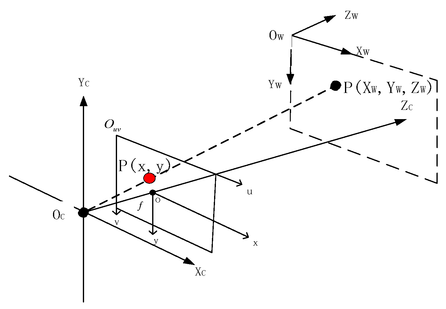
2.1. Coordinate System and Its Transformation Relation

(1)

Coordinate system

The coordinate systems involved in camera imaging are depicted in Figure 1.

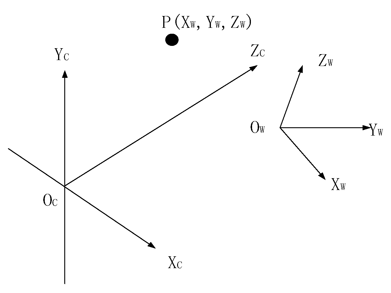
• The world coordinate system: $O_W-X_W{Y}_W{Z}_W$, it describes the position of the measured object in the three-dimensional world. The origin coordinates can be determined according to the specific requirements, and the unit is in meters $(m)$.
• Camera Coordinate System: $O_C-X_C{Y}_C{Z}_C$, the original coordinate system is positioned at the optical center, with the $X_C$-axis and $Y_C$-axis running parallel to the two edges of the image plane. The $Z_C$-axis coincides with the optical axis, and the unit of measurement is meters $(m)$.
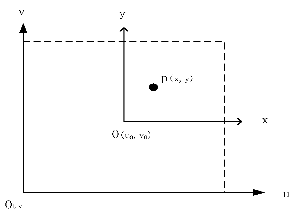
• Pixel Coordinate System: $O_{uv}-uv$, the upper left corner is designated as the origin of the coordinate system for the image plane. The $u$-axis of the pixel coordinate system extends horizontally from left to right, while the $v$-axis extends vertically from top to bottom. The unit of measurement is pixels.
• The coordinate system for the image, referred to as the Image Coordinate System, is defined by the central point of the image plane. The $x$-axis and $y$-axis are aligned in parallel with the $u$-axis and $v$-axis of the pixel coordinate system, respectively. The unit of measurement employed is millimeters.

(2)

Coordinate system transformation relationship

The primary focus of the camera imaging model involves the mapping correlation between the pixel coordinates of an image point $p$ and its corresponding coordinates within three-dimensional space. The camera imaging procedure operates on the principle of pinhole imaging, depicted in Figure 2.

The point $P$ in the figure represents a point in the world coordinate system, with coordinates $(X_W,Y_W,Z_W)$. In the camera coordinate system, the coordinates of point $p$ are $(X_C,Y_C,Z_C)$. The corresponding imaging point of point $p$ in the image is located in the pixel coordinate system with coordinates $(u,v)$, while the coordinates of point $p$ in the image coordinate system are $(x,y)$. The focal length of the camera, denoted as $f$, $f=‖o-O_C‖$, is the distance between $o$ and $O_C$ [12]. The projection transformation from camera coordinates to image coordinates follows specific transformations based on the principles of triangle similarity.

$$\frac{BC}{Ao}=\frac{C{O}_C}{o{O}_C}=\frac{PB}{pA}=\frac{X_C}{x}=\frac{Y_C}{y}=\frac{Z_C}{f}$$

(1)

According to Formula (1):

$$x=f\frac{X_C}{Z_C},y=f\frac{Y_C}{Z_C}$$

(2)

According to Formula (2):

$$Z_C\left[\begin{array}{l}x\\ y\\ 1\end{array}\right]=\left[\begin{array}{cccc}f& 0& 0& 0\\ 0& f& 0& 0\\ 0& 0& 1& 0\end{array}\right]\left[\begin{array}{l}{X}_C\\ Y_C\\ Z_C\\ 1\end{array}\right]$$

(3)

Figure 3 exhibits the process of converting camera coordinates into world coordinates.

The conversion from world coordinates to camera coordinates involves only rotation and translation operations and is considered a rigid transformation. The equation for coordinate transformation is as follows:

$$\left[\begin{array}{l}{X}_C\\ Y_C\\ Z_C\\ 1\end{array}\right]=\left[\begin{array}{cc}R& T\\ 0& 1\end{array}\right]\left[\begin{array}{l}{X}_W\\ Y_W\\ Z_W\\ 1\end{array}\right]$$

(4)

The rotation matrix, denoted as $R$, is a 3 × 3 matrix, and the translation vector, denoted as $T$, is a 3 × 1 vector. The representation of the camera coordinate system’s homogeneous coordinates is denoted as $O_C-X_C{Y}_C{Z}_C$, whereas the homogeneous coordinates of the world coordinate system are denoted as $O_W-X_W{Y}_W{Z}_W$. During the coordinate transformation process, rotation is performed by rotating around the $z$-axis with an angle of $\theta$, and rotating around the $x$ and $y$ axes with angles $\alpha$ and $\beta$, respectively, resulting in the composite rotation matrix $R=R_1{R}_2{R}_3$.

$$R=\left[\begin{array}{ccc}\cos \theta & -\sin \theta & 0\\ \sin \theta & \cos \theta & 0\\ 0& 0& 1\end{array}\right]\left[\begin{array}{ccc}\cos \beta & 0& \sin \beta \\ 0& 1& 0\\ -\sin \beta & 0& \cos \beta \end{array}\right]\left[\begin{array}{ccc}1& 0& 0\\ 0& \cos \alpha & -\sin \alpha \\ 0& \sin \alpha & \cos \alpha \end{array}\right]$$

(5)

$$\left[\begin{array}{l}{X}_C\\ Y_C\\ Z_C\end{array}\right]=R\left[\begin{array}{l}{X}_W\\ Y_W\\ Z_W\end{array}\right]+T$$

(6)

The camera captures two-dimensional images, and the output consists of pictures where pixels are arranged based on their pixel values. As a result, the pixel coordinate system is derived by discretizing the coordinate values and shifting the origin to the center [13].

Figure 4 illustrates the denotation of the pixel coordinate system as $O_{uv}-uv$ and the image coordinate system as $o-xy$. The representation of point p in the pixel coordinate system is indicated as $(u,v)$, and the transformation relationship is expressed as follows:

$$\left\{\begin{array}{l}u=\frac{x}{dx}+u_0\\ v=\frac{y}{dy}+v_0\end{array}\right.$$

(7)

According to the above formula:

$$\left[\begin{array}{l}u\\ v\\ 1\end{array}\right]=\left[\begin{array}{ccc}\frac{1}{dx}& 0& u_0\\ 0& \frac{1}{dy}& v_0\\ 0& 0& 1\end{array}\right]\left[\begin{array}{l}x\\ y\\ 1\end{array}\right]$$

(8)

In the given equation, the physical dimensions along the $x,y$ directions of the pixel are denoted as $1/dx$ and $1/dy$, respectively, whereas $o(u_0,v_0)$ signifies the displacement of the origin on the pixel plane.

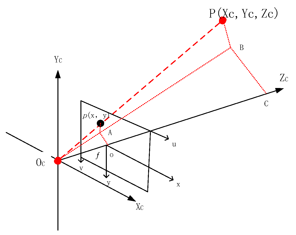
2.2. Camera Imaging Model

(1)

Linear camera model

In an ideal scenario where the distortion resulting from the camera imaging process is neglected, the rectification of a linear camera’s distortion can be achieved by solving the intrinsic and extrinsic parameter matrices of the camera using only the image [14]. This is shown in the following equation:

$$Z_C\left[\begin{array}{l}u\\ v\\ 1\end{array}\right]=\left[\begin{array}{cccc}{f}_x& 0& u& 0\\ 0& f_y& v& 0\\ 0& 0& 1& 0\end{array}\right]\left[\begin{array}{cc}R& T\\ \overrightarrow{0}& 1\end{array}\right]\left[\begin{array}{l}{X}_W\\ Y_W\\ Z_W\\ 1\end{array}\right]$$

(9)

The internal parameter matrix is denoted as Equation (10), while the external parameter matrix is represented as Equation (11):

$$\left[\begin{array}{cccc}{f}_x& 0& u& 0\\ 0& f_y& v& 0\\ 0& 0& 1& 0\end{array}\right]$$

(10)

$$\left[\begin{array}{cc}R& T\\ \overrightarrow{0}& 1\end{array}\right]$$

(11)

(2)

Nonlinear distortion model

Through analyzing the linear camera model, an ideal scenario would reveal a linear correlation, while practical measurement processes often encounter unattainable linearity and inevitable errors [15]. Due to manufacturing process variations, the camera lens generates distortions during the imaging process, leading to nonlinear distortions [16]. Nonlinear distortions can be further categorized into radial and tangential distortions, causing deviations between ideal projected points and actual projected points [17]. Let us assume a point $P$ in the world coordinate system, represented as $P(X_W,Y_W,Z_W)$ in the $O_W-X_W{Y}_W{Z}_W$ coordinates. The corresponding theoretical image coordinate is denoted as $p(x,y)$. However, due to nonlinear distortions introduced by real-world imaging, the actual projected point of this point will deviate.

Expressed as follows is the deviation between the theoretical and actual points when $p(x,y)$ is shifted to point $p\prime (x\prime ,y\prime )$:

$$\left\{\begin{array}{l}x\prime =x+{\delta }_x\\ y\prime =y+{\delta }_y\end{array}\right.$$

(12)

For the nonlinear distortion offset in the $x$ direction, ${\delta }_x$ is used as a representation, while ${\delta }_y$ represents the nonlinear distortion offset in the $y$ direction. In the case of nonlinear distortion offsets, the coefficients $k_1,k_2,k_3$ are employed to denote radial distortion. The expressions for the initial terms in the Taylor expansion are provided below:

$$\left\{\begin{array}{l}x\prime =x(1+k_1{r}^2+k_2{r}^4+k_3{r}^6)\\ y\prime =y(1+k_1{r}^2+k_2{r}^4+k_3{r}^6)\end{array}\right.$$

(13)

The radial distortion coefficients, denoted by $k_1,k_2,k_3$, $r^2=x^2+y^2$.

To ensure comprehensive distortion analysis, it is crucial to incorporate the consideration of tangential distortion. This type of distortion arises mainly from the disparity between the principal point of the optical system and the geometric center. The changes in tangential distortion are comparatively smaller in magnitude than that of radial distortion. The expression for tangential distortion is as follows:

$$\left\{\begin{array}{l}x\prime =x+[2p_{1}y+p_2(r^2+2x^2)]\\ y\prime =y+[p_1(r^2+2y^2)+2p_{2}x]\end{array}\right.$$

(14)

The eccentric distortion coefficients, denoted by $p_1,p_2$, $r^2=x^2+y^2$.

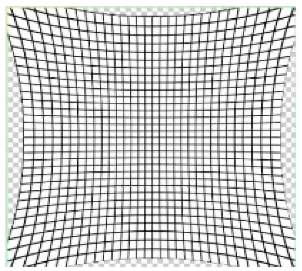
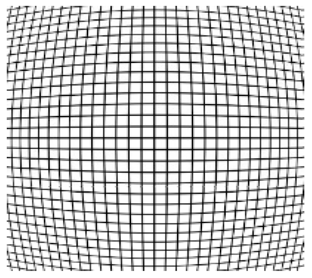
2.3. Distortion Correction

Lens distortion is actually a collective term for inherent perspective distortions in optical lenses [18]. Generally, there are three types of camera distortions:

(1)

Pincushion distortion: The magnification rate in the peripheral regions of the field of view is much larger than that near the optical axis center, commonly found in telephoto lenses [19].

(2)

Barrel distortion: In contrast to pincushion distortion, the magnification rate near the optical axis center is much larger than that in the peripheral regions [20].

(3)

Linear distortion: When the optical axis is not orthogonal to the vertical plane of objects being photographed, the convergence of the far side that should be parallel to the near side occurs at different angles, resulting in distortion. This distortion is essentially a form of perspective transformation, meaning that at certain angles, any lens will produce similar distortions [21].

The types of distortions in a camera are as follows (Figure 5, Figure 6 and Figure 7):

The aforementioned distortions were taken into account during the calibration process [22]. Following the transformation Formulas (13) and (14), undistorted calibration results can be obtained using the following equation.

$$\left[\begin{array}{l}{x}_u\\ y_u\end{array}\right]=[1+k_1(x_d^2+x_d^2)+k_2(x_d^2+x_d^2)+k_3(x_d^2+x_d^2)][x_d{y}_d]+\left[\begin{array}{l}2p_1{x}_d{y}_d+p_2(3x_d^2+y_d^2)\\ p_2(3x_d^2+y_d^2)+2p_2{x}_d{y}_d\end{array}\right]$$

Here, a nonlinear model is introduced to account for distortion in camera calibration. In real-world scenarios, the calibration of distortion serves as an effective means to minimize the influence of distortion, thus safeguarding the precision of the calibration outcomes.

3. Camera Calibration

3.1. Camera Calibration Algorithm

After analyzing the coordinate transformation relationship in photogrammetric measurement and the previously delineated camera distortion model, the calibration of the camera is conducted [23].

First, construct the homograph matrix to establish the relationship between world coordinates and pixel coordinates. This matrix describes the homographs between the target point in the world coordinate system and the image point. Subsequently, solve the initial values for the camera’s intrinsic and extrinsic parameters using orthogonal constraint conditions. Finally, an optimization algorithm is applied to obtain reliable matrices for the intrinsic and extrinsic parameters [24]. According to the camera imaging model and the transformation relationship between pixel coordinates and world coordinates, the expression for the camera imaging model is as follows:

$$s\overline{m}=A[R,T]\overline{M}$$

(15)

In Equation (15), the pixel coordinates of the image are denoted as $\overline{m}$, the world coordinates as $\overline{M}$, the intrinsic matrix as $A$, the extrinsic matrix as $[R,T]$, and the scale factor as $s$. The expression based on Equation (15) is presented in homogeneous coordinates as follows:

$$s\left[\begin{array}{l}u\\ v\\ 1\end{array}\right]=A[\begin{array}{cccc}{r}_1& r_2& r_3& t\end{array}]\left[\begin{array}{l}X\\ Y\\ Z\\ 1\end{array}\right]$$

(16)

Then, the internal parameters of the camera can be expressed as:

$$A=\left[\begin{array}{ccc}{f}_u& \gamma & u_0\\ 0& f_v& v_0\\ 0& 0& 1\end{array}\right]$$

(17)

Since the scale factor $s$ does not alter the homogeneous coordinate values, in Zhang’s calibration method, where pixel coordinates are in two dimensions, we can set $Z=0$. Consequently, Equation (15) can be expressed as follows:

$$s\left[\begin{array}{l}u\\ v\\ 1\end{array}\right]=\lambda A[\begin{array}{cccc}{r}_1& r_2& r_3& t\end{array}]\left[\begin{array}{l}X\\ Y\\ 0\\ 1\end{array}\right]=\lambda A[\begin{array}{ccc}{r}_1& r_2& t\end{array}]\left[\begin{array}{l}X\\ Y\\ 1\end{array}\right]$$

(18)

Given that $\lambda =1/s$, and the homographs matrix is denoted as $H$, we can set $H=\lambda A[\begin{array}{ccc}{r}_1& r_2& t\end{array}]$. Consequently, the camera model can be represented by Equation (19):

$$s\overline{m}=H\overline{M}$$

(19)

Let $H=[\begin{array}{ccc}{h}_1& h_2& h_3\end{array}]=\lambda A[\begin{array}{ccc}{r}_1& r_2& t\end{array}]$, the $r$ vector is represented by the homologous matrix $H$ as follows:

$$\left\{\begin{array}{l}{r}_1=\frac{1}{\lambda }{A}^{-1}{h}_1\\ r_2=\frac{1}{\lambda }{A}^{-1}{h}_2\end{array}\right.$$

(20)

According to orthogonality, the vector’s own constraints are expressed as:

$$\left\{\begin{array}{l}{r}_1^2=r_2^2=r_3^2=1\\ r_1{r}_2=r_1{r}_3=r_2{r}_3=0\end{array}\right.$$

(21)

$$\left\{\begin{array}{l}{r}_1^T{r}_2=0\\ ‖r_1‖=‖r_2‖=1\end{array}\right.$$

(22)

By bringing Formula (21) into Formula (22), we can obtain:

$$\left\{\begin{array}{l}{h}_1^T{A}^{-T}{A}^{-1}{h}_2=0\\ h_1^T{A}^{-T}{A}^{-1}{h}_1=h_2^T{A}^{-T}{A}^{-1}{h}_2\end{array}\right.$$

(23)

For each feature point in the target image, we can derive two equations. By selecting four points from the target image, as long as three of them are not collinear, the matrix $H$ can be computed. Consequently, a matrix $H$ can be derived, with the following expression:

$$s\left[\begin{array}{l}u\\ v\\ 1\end{array}\right]=\left[\begin{array}{ccc}{h}_{11}& h_{12}& h_{13}\\ h_{21}& h_{22}& h_{23}\\ h_{31}& h_{32}& h_{33}\end{array}\right]\left[\begin{array}{l}X\\ Y\\ 1\end{array}\right]$$

(24)

The expression for Equation (24) can be transformed into a set of equations as follows:

$$\left\{\begin{array}{l}uX{h}_{31}+uY{h}_{32}+u{h}_{33}=h_{11}X+h_{12}Y+h_{13}\\ vX{h}_{31}+vY{h}_{32}+v{h}_{33}=h_{21}X+h_{22}Y+h_{23}\end{array}\right.$$

(25)

Expressing Equation (25) in matrix form, while setting $h\prime ={[\begin{array}{ccccccccc}{h}_{11}& h_{12}& h_{13}& h_{21}& h_{22}& h_{23}& h_{31}& h_{32}& h_{33}\end{array}]}^T$, yields the following matrix expression:

$$\left[\begin{array}{ccccccccc}X& Y& 1& 0& 0& 0& -uX& -uY& -u\\ 0& 0& 0& X& Y& 1& -vX& -vY& -v\end{array}\right]h\prime =0$$

(26)

By applying the orthogonality condition stated in Equation (23), we can construct a matrix of homographs to determine the camera’s intrinsic and extrinsic parameters. Since $A^{-T}{A}^{-1}$ is present within Equation (23), the following matrix is formed by setting $B=A^{-T}{A}^{-1}$. Its expression is as follows:

$$B=A^{-T}{A}^{-1}=\left[\begin{array}{ccc}{B}_{11}& B_{12}& B_{13}\\ B_{21}& B_{22}& B_{23}\\ B_{31}& B_{32}& B_{33}\end{array}\right]$$

(27)

Bringing Equation (17) into Equation (27) yields the following expression:

$$B=A^{-T}{A}^{-1}=\left[\begin{array}{ccc}\frac{1}{f_u^2}& \frac{\gamma }{f_u^2{f}_v}& \frac{v_0\gamma -u_0{f}_v}{f_u^2{f}_v}\\ -\frac{\gamma }{f_u^2{f}_v}& \frac{{\gamma }^2}{f_u^2{f}_v^2}+\frac{1}{f_v^2}& -\frac{\gamma (v_0\gamma -u_0{f}_v)}{f_u^2{f}_v^2}-\frac{v_0}{f_v^2}\\ \frac{v_0\gamma -u_0{f}_v}{f_u^2{f}_v}& -\frac{\gamma (v_0\gamma -u_0{f}_v)}{f_u^2{f}_v^2}-\frac{v_0}{f_v^2}& \frac{{(v_0\gamma -u_0{f}_v)}^2}{f_u^2{f}_v^2}+\frac{v_0}{f_v^2}+1\end{array}\right]$$

The matrix $B$ possesses a symmetric structure and can be represented by Equation (28):

$$b={\left[\begin{array}{cccccc}{B}_{11}& B_{12}& B_{22}& B_{13}& B_{23}& B_{33}\end{array}\right]}^T$$

(28)

According to the orthogonal constraint: $h_i^{T}B{h}_j=v_{ij}^{T}b$, we can obtain:

$$v_{ij}={\left[\begin{array}{cccccc}{h}_{i1}{h}_{j1}& h_{i1}{h}_{j2}+h_{i2}{h}_{j1}& h_{i2}{h}_{j2}& h_{i3}{h}_{j1}+h_{i1}{h}_{j3}& h_{i3}{h}_{j2}+h_{i2}{h}_{j3}& h_{i3}{h}_{j3}\end{array}\right]}^T$$

The equation’s expression of orthogonality constraint results in $v_{12}^{T}b=0$.

Similarly, based on another constraint, it can be represented as ${(v_{11}-v_{22})}^{T}b=0$. These two constraints can be expressed in matrix form, and their expression is as follows:

$$\left[\begin{array}{c}{v}_{12}^T\\ {(v_{11}-v_{22})}^T\end{array}\right]b=0$$

(29)

During the camera calibration process, for each image, we can obtain a homographs matrix $H$. Based on Equation (29), each of these matrices can be used to form the system of equations described in the equation. According to Equation (28), $v_{ij}$ has six unknowns; thus, at least six sets of equations need to be established in order to solve them. In practical experiments, there are often redundant data available, allowing for the calculation of the $B$ matrix. By solving the $B$ matrix using the Cholesky (square root) method and taking its inverse, we can obtain the camera’s intrinsic parameters. Its expression is given by Equation (30).

$$\left\{\begin{array}{l}{v}_0=\frac{(B_{12}{B}_{13}-B_{11}{B}_{23})}{(B_{11}{B}_{22}-B_{12}^2)}\\ \lambda =\frac{B_{33}-\left[B_{13}^2+v_0(B_{12}{B}_{13}-B_{11}{B}_{23})\right]}{B_{11}}\\ f_u=\sqrt{\frac{\lambda }{B_{11}}}\\ f_v=\sqrt{\frac{\lambda B_{11}}{B_{11}{B}_{22}-B_{12}^2}}\\ \gamma =-\frac{B_{12}{f}_u^2{f}_v}{\lambda }\\ u_0=\frac{v_0\gamma }{f_v}-\frac{B_{13}{f}_u^2}{\lambda }\end{array}\right.$$

(30)

Then, according to $H=[\begin{array}{ccc}{h}_1& h_2& h_3\end{array}]=\lambda A[\begin{array}{ccc}{r}_1& r_2& t\end{array}]$, the external parameters are simplified, and the result is expressed as Equation (31):

$$\left\{\begin{array}{c}{r}_1=\lambda A^{-1}{h}_1\\ r_2=\lambda A^{-1}{h}_2\\ r_3=r_1{r}_2\\ t=\lambda A^{-1}{h}_3\\ \lambda =\frac{1}{‖A^{-1}{h}_1‖}=\frac{1}{‖A^{-1}{h}_2‖}\end{array}\right.$$

(31)

Solving Equations (30) and (31) allows for the determination of both the camera’s internal and external parameters.

3.2. Binocular Stereo Calibration Method

Based on the camera imaging model, Equation (32) can be derived when considering the internal and external parameter matrices of the left and right cameras in a binocular vision system portrayed as $R_1$, $T_1$, $R_2$, and $T_2$, respectively. Furthermore, point $P$ in world coordinates are $P_W$, while its coordinates on the imaging plane of the left camera and the right camera are $p_1$ and $p_2$, respectively.

$$\left\{\begin{array}{c}{p}_1=R_1{P}_W+T_1\\ p_2=R_2{P}_W+T_2\end{array}\right.$$

(32)

Equation (33) is obtained by eliminating $P_W$ from the upper equations:

$$p_2=R_2{R}_1^{-1}{p}_1+T_2-R_2{R}_1^{-1}{T}_1=R{p}_1+T$$

(33)

Equation (33) defines $R$ as the rotation matrix relating the two cameras and $T$ as the translation vector representing the spatial relationship between the cameras. Consequently, the positional correlation between the left and right cameras is articulated through Equation (34).

$$\left\{\begin{array}{l}R=R_2{R}_1^{-1}\\ T=T_2-R_2{R}_1^{-1}{T}_1\end{array}\right.$$

(34)

Based on Equation (34), the individual calibration of the internal and external parameters for the left and right cameras enables the definition of their positional relationship. This process completes the stereo calibration for the binocular vision system. Subsequently, intelligent optimization algorithms are utilized to enhance the obtained internal and external parameters, as they may not be optimal.

4. Camera Parameter Optimization Algorithm

The Zhang’s calibration method yields unsatisfactory results when multiple images are used as input, with poor performance due to suboptimal initial values and noise-contaminated data. In order to tackle this issue, the linear model solution is utilized as the starting point for optimization, aiming to enhance the resilience of conventional optimization approaches [25]. However, these drawbacks require additional input constraints to obtain more accurate parameter results, making the traditional calibration process more complex and impractical. Hence, this section primarily utilizes intelligent optimization algorithms to optimize the method and address the aforementioned limitations.

Assuming there exist n template images depicting planar surfaces, with each image containing m calibration points within the identical environment, the formulation of the objective function is presented as follows:

$$f_{obj}=\min {\displaystyle \sum _{i=1}^n{\displaystyle \sum _{j=1}^m‖{\widehat{p}}_{ij}-p(M_A,k_1,k_2,k_3,p_1,p_2,R_i,T_i,P_j)‖}}$$

(35)

The pixel coordinates of the $j$ calibration point in the $i$ image are represented by $p_{ij}$ in the objective function, whereas $k_1,k_2,k_3,p_1,p_2$ represents the distortion parameters, and $R_i,T_i$ denotes the rotation and translation matrix corresponding to the $i$ image. By utilizing optimization algorithms to optimize the calibration objective function based on Equation (35), the optimal solution for the camera calibration parameters can be obtained.

4.1. Honey Badger Algorithm

The Honey Badger Algorithm (HBA) presents a pioneering heuristic optimization approach inspired by the foraging behavior of honey badgers, which has devised an efficient search strategy for addressing mathematical optimization problems. The key principle revolves around the honey badger’s capacity to locate beehives through actions such as sniffing, digging, and following honeyguide birds, categorized as the excavation mode and the honey mode, respectively. During the excavation mode, the honey badger uses its keen sense of smell to estimate the beehive’s location and chooses a suitable spot for excavation upon nearing the hive. Conversely, in the honey mode, the honey badger directly relies on the guidance of the honeyguide bird to find the beehive, ultimately yielding the optimal outcome.

The optimization of camera parameters based on the honey badger algorithm involves establishing an objective function using the residuals between the actual image coordinates $(x,y)$ of calibration points and the projected coordinates $(x^{\prime },y^{\prime })$ calculated from the camera model.

$$f(X)={\displaystyle \sum _i^N[{(x-x^{\prime })}^2+{(y-y^{\prime })}^2]}$$

(36)

By utilizing the excavation mode and honey mode to minimize the value of $f(X)$, an optimal set of parameters is obtained, achieving the optimization of camera parameters.

Here, $X$ represents the parameter to be optimized, specifically $X=[f_x,f_y,C_x,C_y,k_1,k_2,k_3,p_1,p_2]$, with the parameter’s search range set as $[X_{up},X_{down}]$, as shown below:

$$X_{up}=[f_x+3,f_y+3,C_x+2,C_y+2,k_1+0.1,k_2+0.02,k3+0.002,p_1+2\times {10}^{-5},p_2+0.02]$$

$$X_{down}=[f_x-3,f_y-3,C_x-2,C_y-2,k_1-0.1,k_2-0.02,k3-0.002,p_1-2\times {10}^{-5},p_2-0.02]$$

The population of honey badgers, with a size of N, representing the optimization of D parameters, can be expressed as follows:

$$\left[\begin{array}{ccccc}{x}_{11}& x_{12}& x_{13}& \cdots & x_{1D}\\ x_{21}& x_{22}& x_{23}& \cdots & x_{2D}\\ ⋮& ⋮& ⋮& & ⋮\\ x_{N1}& x_{N2}& x_{N3}& \cdots & x_{ND}\end{array}\right]$$

(37)

The position of the i honey badger is:

$${\mathrm{x}}_i=[x_{i1},x_{i2},x_{i3},\cdots ,x_{iD}]$$

(38)

The flowchart of the honey badger algorithm is as follows (Figure 8):

The algorithm steps are as follows:

Step 1: The initialization phase entails setting the population size N and determining the corresponding positions of the honey badgers.

$${\mathrm{x}}_i=l{b}_i+r_1\times (u{b}_i-l{b}_i)$$

(39)

where $r_1$ denotes a random number within the range of 0 to 1, $l{b}_i$ signifies the lower boundary of the search domain, and $u{b}_i$ denotes the upper boundary of the search domain.

Determine the maximum number of iterations, denoted as T, as well as parameters C and $\beta$.

Step 2: Specifying the intensity I. The intensity is linked to the prey’s concentration and the spatial separation between the prey and honey badgers. $I_i$ denotes the olfactory potency of the prey, where a high olfactory strength results in fast movement, whereas a low olfactory strength leads to slow movement.

$$I_i=r_2\times \frac{S}{4\pi d_i^2}$$

(40)

$$S={(x_i-x_{i+1})}^2$$

(41)

$$d_i=x_{prey}-x_i$$

(42)

In this section, the symbol $r_2$ represents a random number between 0 and 1, S denotes the source strength or concentration strength, and $d_i$ represents the distance between the i-th honey badger and its prey.

Step 3: Enhancing the density factor. The density factor $\alpha$ controls the dynamic randomization process, facilitating a seamless transition from exploration to exploitation.

$$\alpha =C\times \exp (\frac{-t}{t_{\max }})$$

(43)

Step 4: Escape from local optima. This step is aimed at escaping from local optima regions. The search algorithm employs a flag F to alter the search direction, facilitating an extensive exploration of the search space.

Step 5: Adjusting individual positions. The process of updating positions comprises two components: the “excavation phase” and the “honey collection phase”.

Excavation phase:

$$x_{new}=x_{prey}+F\times \beta \times I\times x_{prey}+F\times r_3\times \alpha \times d_i\times \left|\cos (2\pi r_4)\times [1-\cos (2\pi r_5)]\right|$$

In this context, $x_{new}$ signifies the revised location of the honey badger individual, while $x_{prey}$ denotes the prey’s position.

Meanwhile, $\beta$ signifies the honey badger’s capability to obtain physical items, where $\beta \ge 1$ with a default of 6, and $d_i$ denotes the distance between the i-th honey badger and the prey. Additionally, $r_3,r_4,r_5,r_6,r_7$ are random numbers between 0 and 1.

$$F=\left\{\begin{array}{l}1 if r_6\le 0.5\\ -1 else\end{array}\right.$$

(44)

Honey gathering stage:

$$x_{new}=x_{prey}+F\times r_7\times \alpha \times d_i$$

(45)

$x_{new}$ represents the revised location of the honey badger individual, while $x_{prey}$ indicates the position of the prey, which represents the globally optimal position. The variable d represents the distance between the i-th honey badger and the prey. The value of F can be calculated using Equation (44), and the value of $\alpha$ can be derived from Equation (43).

4.2. Improved Differential Evolution Particle Swarm Algorithm

Considering the limitations of the honey badger algorithm, including rapid convergence, low accuracy of convergence, tendency to diverge, and decreasing population diversity as iterations increase, the particle swarm optimization algorithm incorporates the differential evolution algorithm to overcome these limitations. In this enhanced algorithm, differential evolution mutation and crossover operations are integrated into the particle swarm algorithm at each iteration. This modification aims to preserve the diversity of the particle population and improve the selection of the optimal particle in each iteration, ultimately leading to enhanced performance.

4.2.1. Principle of Differential Evolution Algorithm

The main components of the differential evolution (DE) algorithm include mutation, crossover, and selection operations. Within this algorithm, a diverse subset of individuals is randomly chosen to form the variance vector. Subsequently, an additional individual is selected and incorporated into the variance vector to produce an experimental individual. The crossover operation is then executed between the original individual and the respective experimental individual, perturbing the existing population and extending the exploration range. Ultimately, a selection process takes place between the original and offspring individuals, retaining the individuals that satisfy the criteria for the subsequent generation population.

(1)

The initialization of the population

The population of size $(NP,D)$ is randomly generated in the solution space. Each individual, denoted by the i-th element, is given a random value within the predefined range.

$$X_i(G)=\{x_{i1}(G),x_{i2}(G),\cdots ,x_{iD}(G)\}, i=1,2,\cdots ,NP$$

(46)

Within the context of this study, the value of $NP$ corresponds to the population size, while $D$ represents the number of decision variables. Each individual within the initial population is generated in the range $[x_{\min },x_{\max }]$ according to Equation (46).

$$x_{iD}(0)=x_{\min }+rand(0,1)\ast (x_{\max }-x_{\min })$$

(47)

In the above equation, the variable $G$ indicates the $G$ generation, and $[x_{\min },x_{\max }]$ represents the search space domain of the decision variables.

(2)

Variation operation

The mutation operation is employed in the process of $G$ evolution to generate the mutation vector $V_i(G)$ for each individual $X_i(G)$ in the population of the current generation. The calculation of the mutation vector varies depending on the chosen mutation strategy, and the subsequent section outlines five frequently employed mutation strategies.

$$\begin{array}{l}DE/rand/1:\\ \hspace{1em}{V}_i(G)=X_{r1}(G)+F\cdot (X_{r2}(G)-X_{r3}(G))\\ DE/best/1:\\ \hspace{1em}{V}_i(G)=X_{best}(G)+F\cdot (X_{r1}(G)-X_{r2}(G))\\ DE/rand-to-best/1:\\ \hspace{1em}{V}_i(G)=X_i(G)+F\cdot (X_{best}(G)-X_i(G))+F\cdot (X_{r1}(G)-X_{r2}(G))\\ DE/best/2:\\ \hspace{1em}{V}_i(G)=X_{best}(G)+F\cdot (X_{r1}(G)-X_{r2}(G))+F\cdot (X_{r3}(G)-X_{r4}(G))\\ DE/rand/2:\\ \hspace{1em}{V}_i(G)=X_{r1}(G)+F\cdot (X_{r2}(G)-X_{r3}(G))+F\cdot (X_{r4}(G)-X_{r5}(G))\end{array}$$

(48)

In the above equation, $r_1,r_2,r_3,r_4,r_5$ is a mutually exclusive random integer within the range $[1,NP]$ and different from the index $i$. The scaling factor $F$ is a positive controlling parameter of the differential vector. $X_{best}(G)$ represents the best individual vector in the $G$ generation population with the optimal fitness value.

(3)

Crossover Operation

For each pair of target vector $X_i(G)$ and mutation vector $V_i(G)$, a trial vector is generated through crossover. The differential evolution method employs a binomial crossover defined as follows in Equation (49): $U_i(G)=(u_i(G),u_i(G),\cdots ,u_I(G))$.

$$u_i(G)=\left\{\begin{array}{l}{v}_i(G),(ran{d}_j(0,1)\le CR)or(j=j_{rand})\\ x_i(G),otherwise\end{array}\right.j=1,2,\cdots ,D$$

(49)

Among them, CR is a specified constant crossover probability between $(0,1)$, and $j_{rand}$ is a randomly selected integer within the range $[1,D]$.

(4)

Selection Operation

In the differential evolution method, a greedy selection rule is utilized to determine the offspring. This rule involves comparing the fitness values of the trial individuals with the target individuals and selecting the superior individuals to be inherited in the subsequent generation.

$$X_i(G+1)=\left\{\begin{array}{l}{U}_i(G),if(f(U_i(G))\le f(X_i(G)))\\ X_i(G),otherwise\end{array}\right.$$

(50)

Among these, $f(\cdot )$ denotes the fitness value of the objective function for both the target individual and the trial individual in the $G$ generation. The above operations are repeated in each generation until certain specific termination conditions are met.

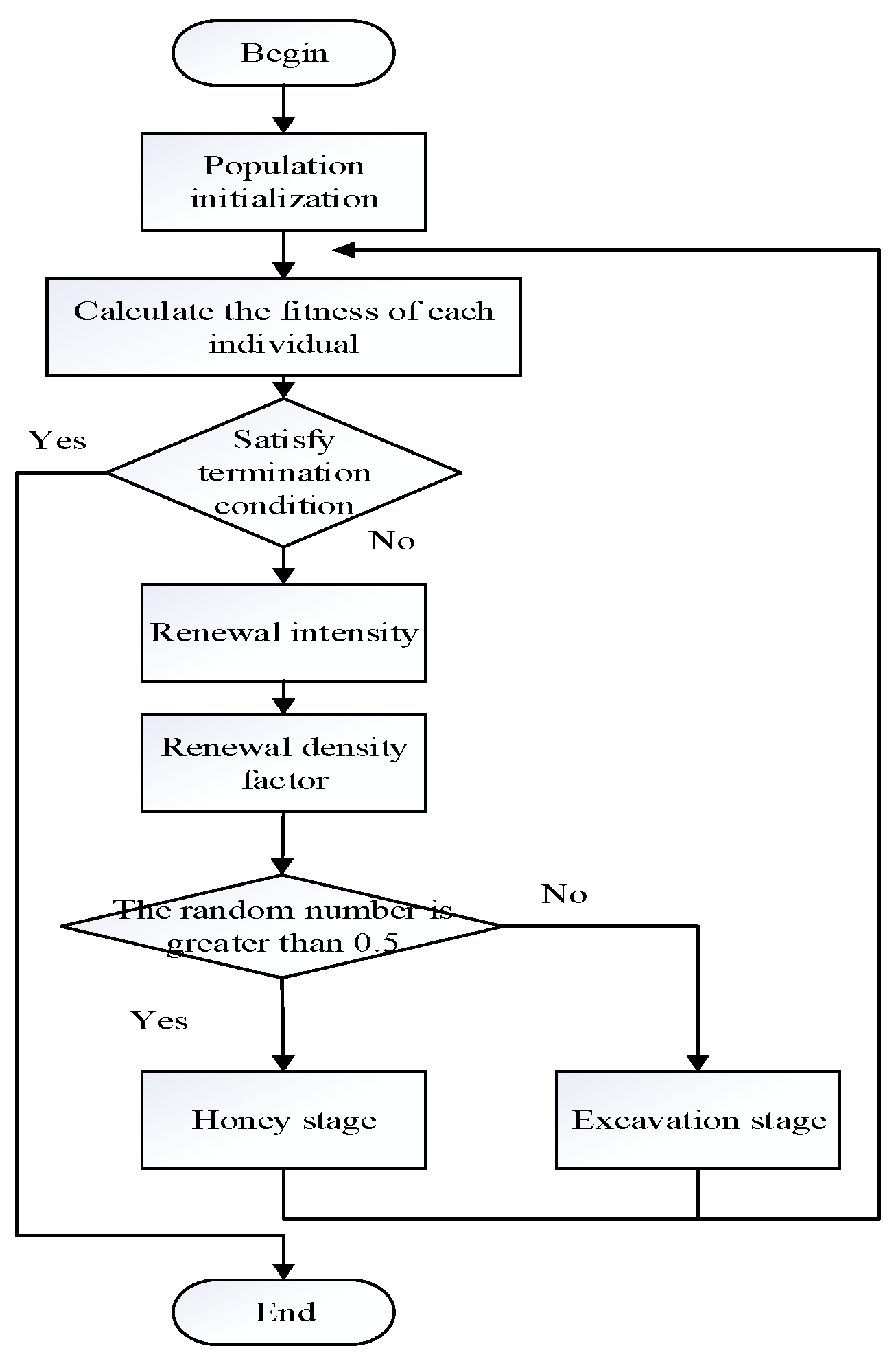
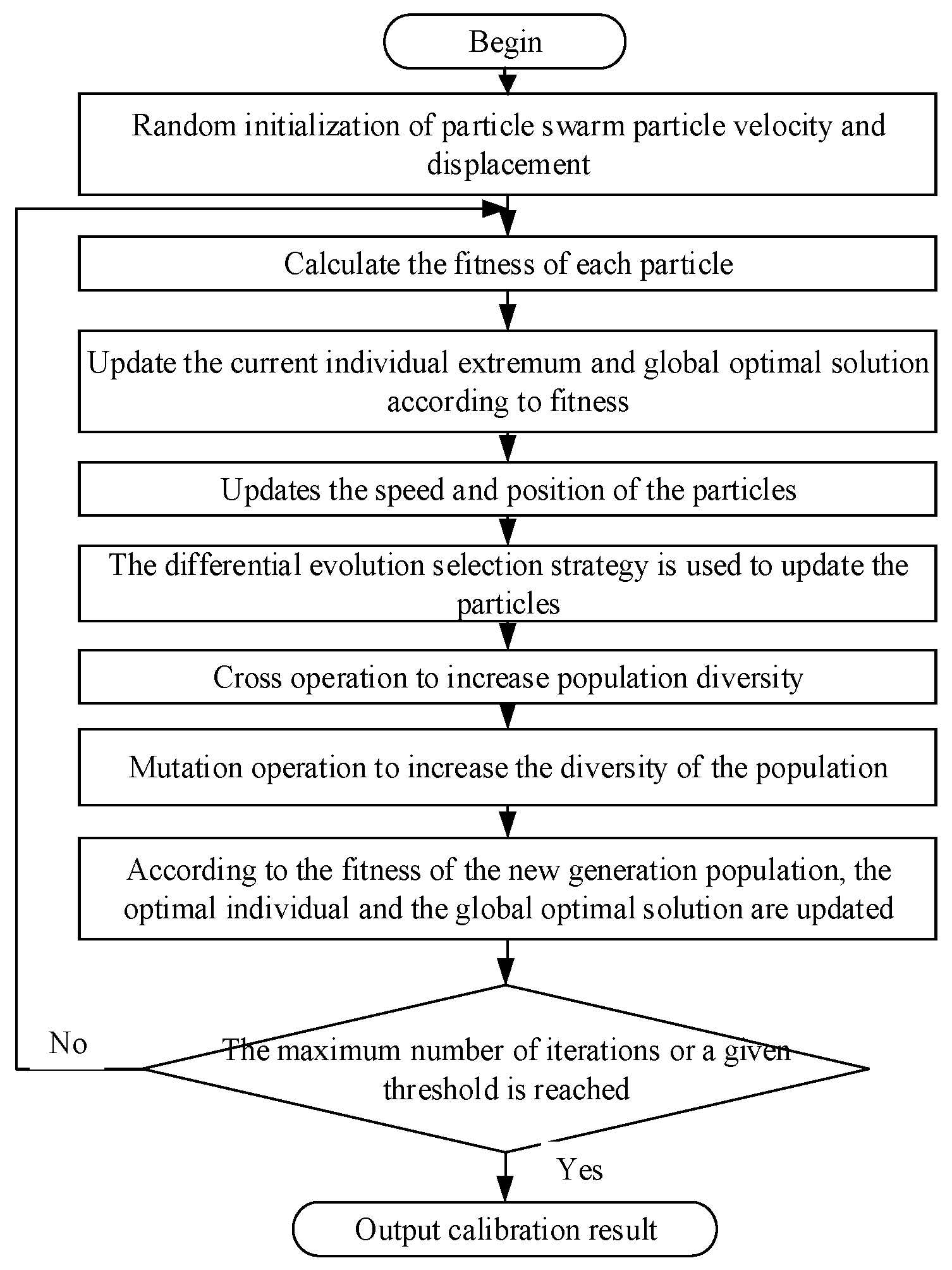
4.2.2. Improved Differential Evolution Particle Swarm Hybrid Optimization Algorithm Design

The population size in the context of the differential evolution algorithm is denoted by N, with each individual possessing a multidimensional vector, which is expressed as the target vector and the trial vector: $X_i^t=(x_{i1}^t,x_{i2}^t,\dots ,x_{iD}^t)$, $V_i^t=(v_{i1}^t,v_{i2}^t,\dots ,v_{iD}^t)$. The population is initialized as $S=\left\{X_1,X_2,\dots ,X_D\right\}$, where T represents each target vector. Therefore, the mutation operation can be improved as follows.

$$V_i^T=x_{best}^t+f(x_{r2}^t-x_{r3}^t)$$

(51)

$$V_i^T=x_{r1}^t+f(x_{r2}^t-x_{r3}^t)$$

(52)

$$V_i^T=x_i^t+f_1(x_{best}^t-x_i^t)+f_2(x_{r1}^t-x_{r2}^t)$$

(53)

$$V_i^T=x_{\mathrm{best}}^t+f(x_{r1}^t+x_{r2}^t-x_{r3}^t-x_{r4}^t)$$

(54)

$$V_i^T=x_{\mathrm{r}1}^t+f(x_{r2}^t+x_{r3}^t-x_{r4}^t-x_{r5}^t)$$

(55)

The equation above introduces $f$ as the mutation parameter, which serves to control the differential speed, while $r_1,r_2,r_3,r_4,r_5$ represents distinct random integers falling within the range of $[1,N]$. The population iteration algorithm incorporates a mutation method to enhance population diversity, ensuring that mutation takes place after each iteration. Moreover, it integrates crossover and selection operations to facilitate the selection of the optimal individual in each iteration.

The Figure 9 depicts the flowchart of the enhanced algorithm for differential evolution particle swarm optimization:

The algorithm implementation steps are as follows:

Step 1: Using calibration algorithm, obtain the coordinates $(x^{\prime },y^{\prime })$ of calibration points and camera parameters $f_x,f_y,C_x,C_y,k_1,k_2,k_3,p_1,p_2$.

Step 2: A group of particles is initialized and distributed throughout the search space, with each particle possessing flight velocity denoted as $V_i$ and position represented as $X_i$. Set the population size $N$, parameter search range, maximum flight velocity $V_{up}$, inertia weight coefficient $\omega$, individual learning factor $c_1$, social learning factor $c_2$, and other parameters. Define the search range of the parameters as $[X_{up},X_{down}]$.

Step 3: An enhanced dynamic adjustment strategy is introduced for the modification of the algorithm’s weights $w$, mutation control parameter $f$, and crossover control parameter $CR$. The maximum number of iterations ${\lambda }_{\max }$ and the current iteration count $\lambda$ are determined based on the upper and lower limits of the parameters specified in Step 2:

$$\delta (w,f,CR)={\delta }_{\max }-\frac{{\delta }_{\max }-{\delta }_{\min }}{{\lambda }_{\max }}\lambda$$

(56)

Step 4: The fitness value of each particle is computed, and the fitness evaluation can be represented by Equation (57).

$$fitness=\min {\displaystyle \sum _{i=1}^m\sqrt{{\left(u_i-x_i\right)}^2+{\left(v_i-y_i\right)}^2}}$$

(57)

Step 5: The current individual extreme value $P_i^t$ for each particle is updated, and the best individual extreme value is recorded as the current global optimal solution $P_g^t$.

Step 6: Each particle updates its flight velocity and position information. The update equations for flight velocity and position information in the d-th dimension are as follows:

$$v_{id}^{t+1}=\omega v_{id}^t+c_1{r}_1(p_{id}^t-x_{id}^t)+c_2{r}_2(p_{gd}^t-x_{id}^t)$$

$$x_{id}^{t+1}=x_{id}^t+v_{id}^{t+1}$$

where $i=1,2,\dots ,N$ and $d=1,2,\dots ,D$, $v_{id}^{t+1}$ and $x_{id}^{t+1}$, respectively represent the flight velocity and position information of the $i$ particle in the $t+1$ generation.

Step 7: Executing the crossover operation enhances population diversity and promotes the adaptation of exceptional individuals.

Step 8: The mutation operation is performed to generate excellent individuals, with a higher probability of mutation for individuals with lower fitness.

Step 9: Updating the entire population is based on the new fitness values, which involves the update of individual best and global best.

Step 10: Checking if the termination condition is met to determine whether to output the results; if the condition is met, the results will be outputted. If not, the process will return to Step 2 for additional iterations.

5. Experimental Comparison and Result Analysis

Using Zhang’s calibration method, the camera was calibrated to obtain the parameters necessary for rectifying the captured images. This process ensured the precise acquisition of pixel coordinates for the chessboard pattern captured by both the left and right cameras. A binocular stereo vision model was then employed to determine the world coordinates of the chessboard pattern. The obtained world coordinates were used as input, while the theoretical world coordinates were used as output. For data computation, a comparative analysis was conducted using different optimization algorithms, including genetic algorithm, particle swarm optimization algorithm, honey badger optimization algorithm, and an enhanced hybrid optimization algorithm that combines differential evolution and particle swarm optimization algorithm.

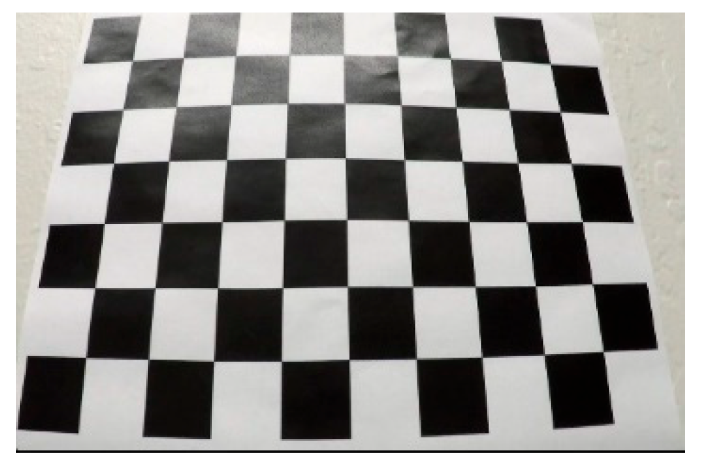
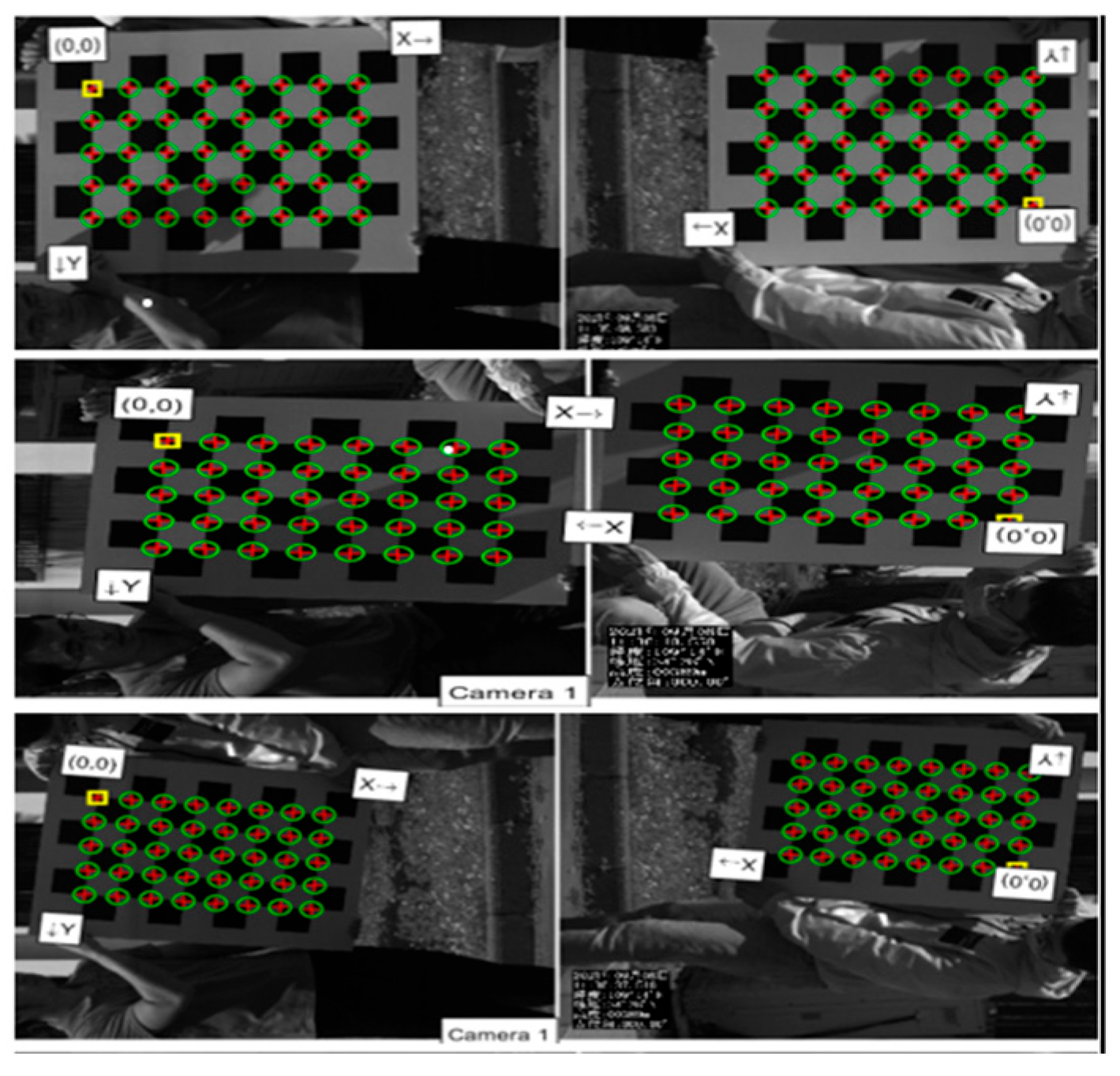
5.1. Procedure of Test

Step 1: Multiple calibration board images were captured using the experimental equipment. Subsequently, functions such as “findChessboardCorners”, “calibrateCamera”, and “stereoRectify” from the OpenCV library were invoked in C++ to solve for the camera’s intrinsic and extrinsic parameters.

Step 2: Multiple sets of captured images were selected. Using OpenCV, pixel coordinates were first determined, followed by the calculation of world coordinates. Figure 10 depicts the calibration board employed in the experiment, which consists of a total of 40 corners. It was manufactured using photolithography techniques, with a fabrication error within 1 millimeter. Each chessboard square measures 80 mm × 80 mm, resulting in a total chessboard size of 800 × 600.

Step 3: The collected calibration images were input into the camera calibration data processing module, resulting in initial data after calibration, including initial values for various types of distortion coefficients.

Step 4: Different optimization techniques were applied to optimize the initial calibration parameters and obtain the global optimum solution.

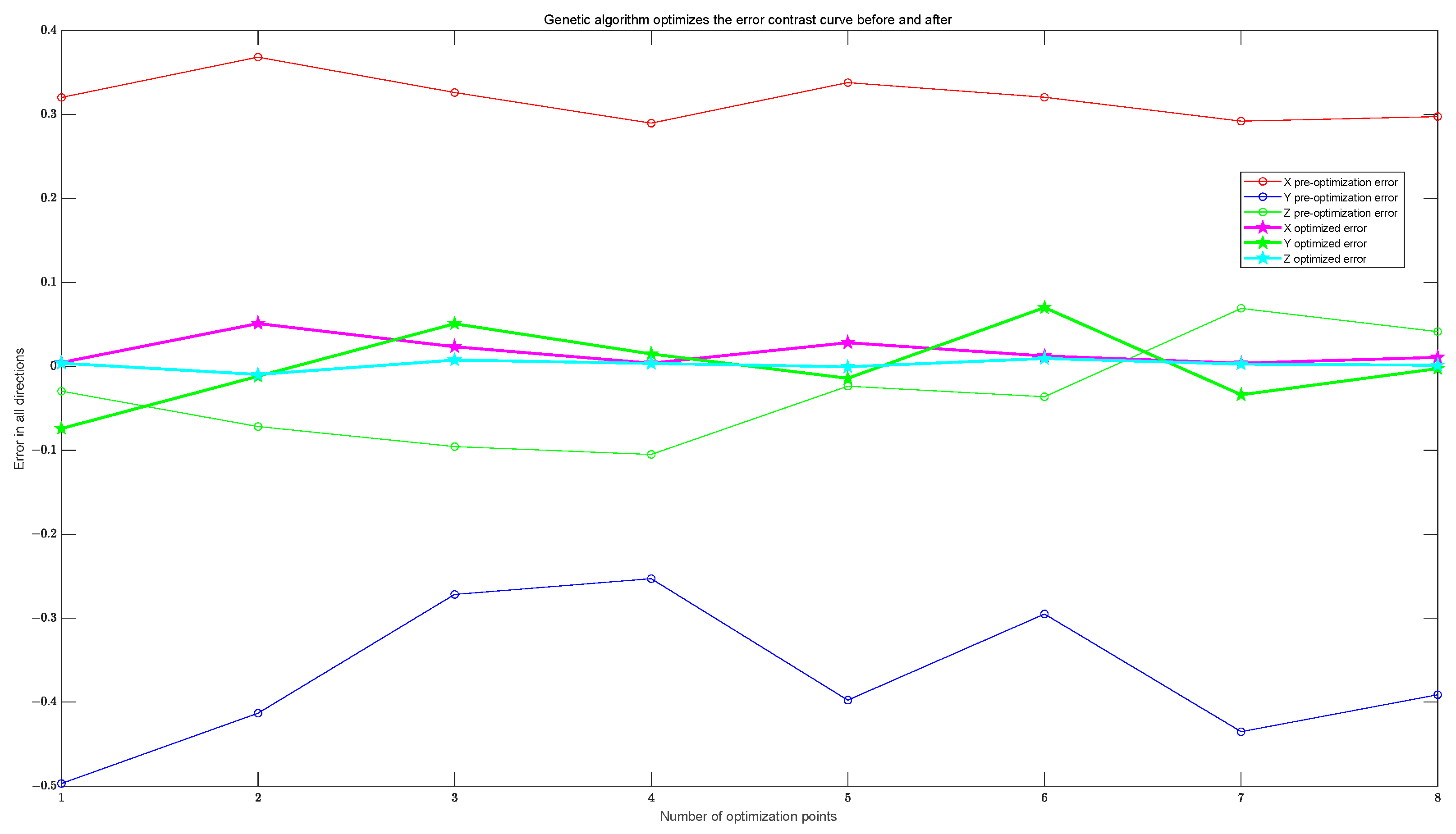
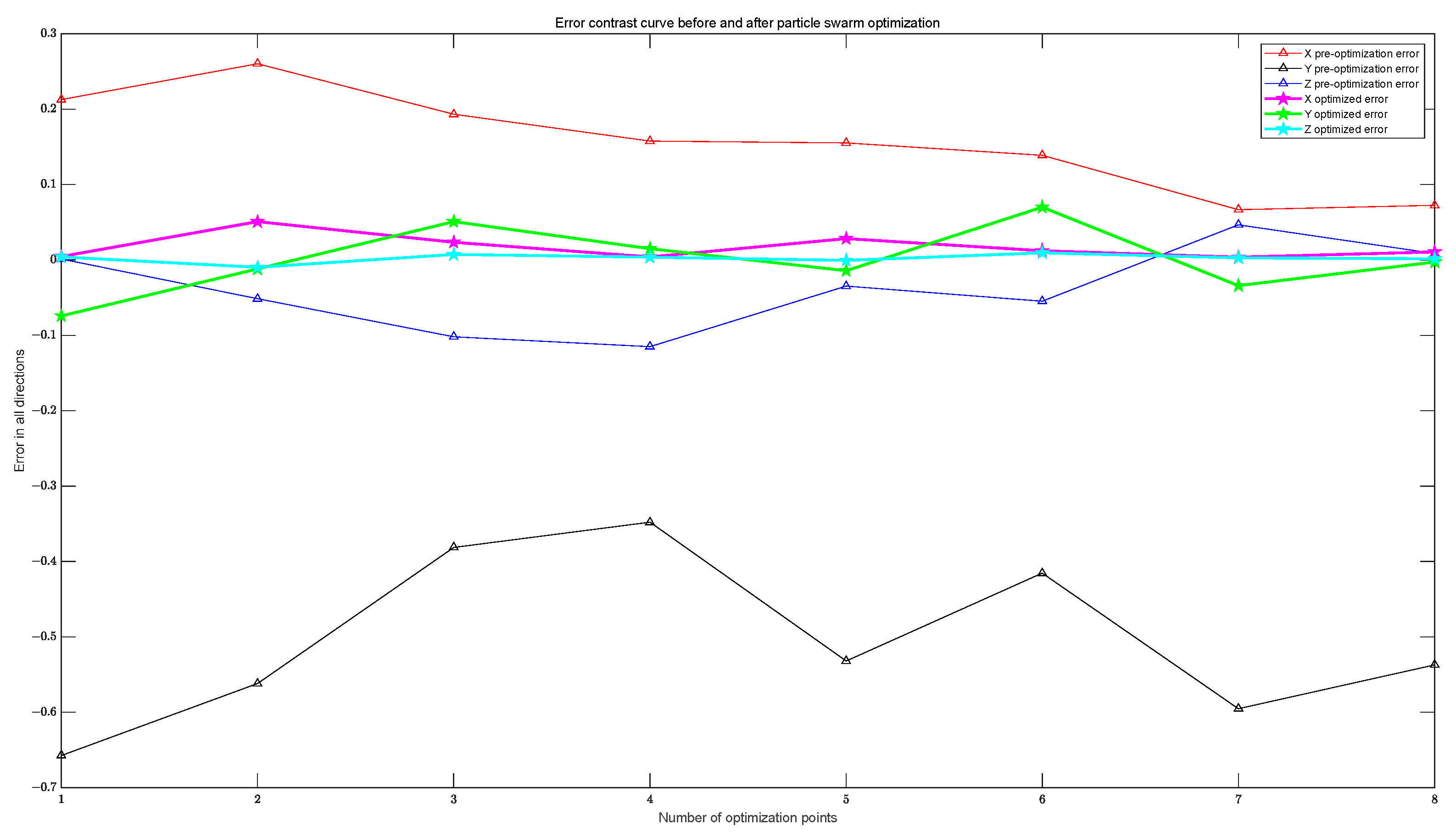
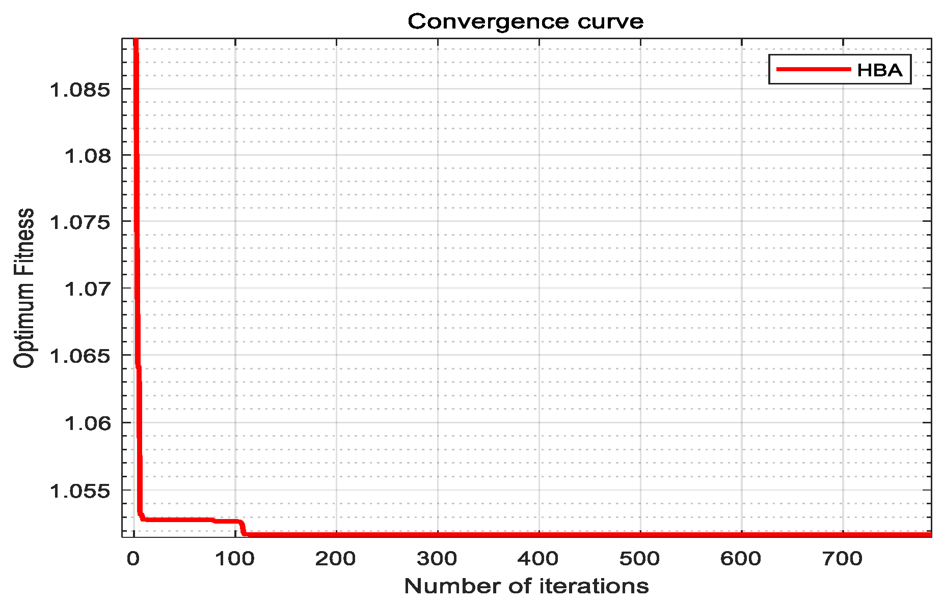
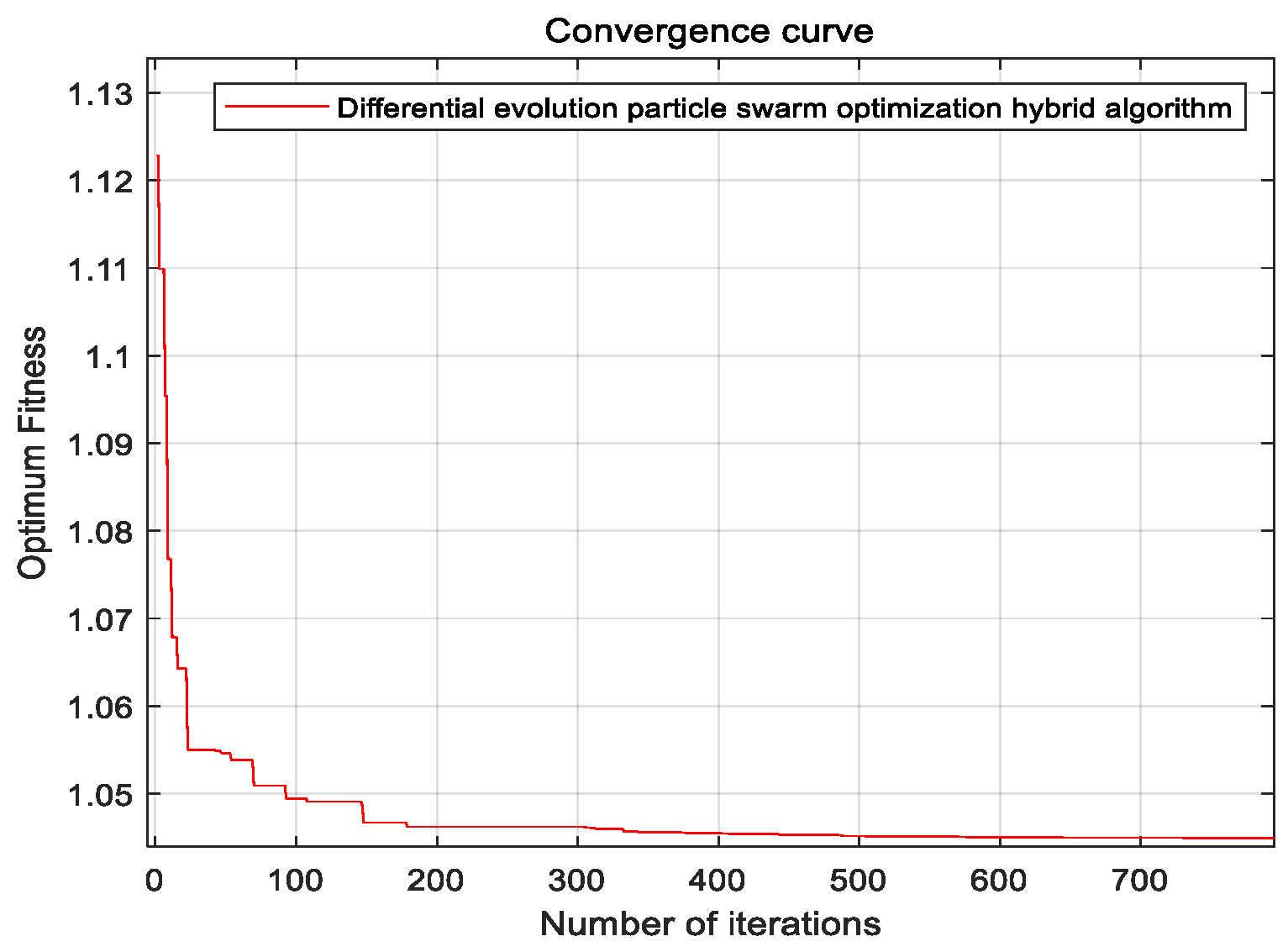
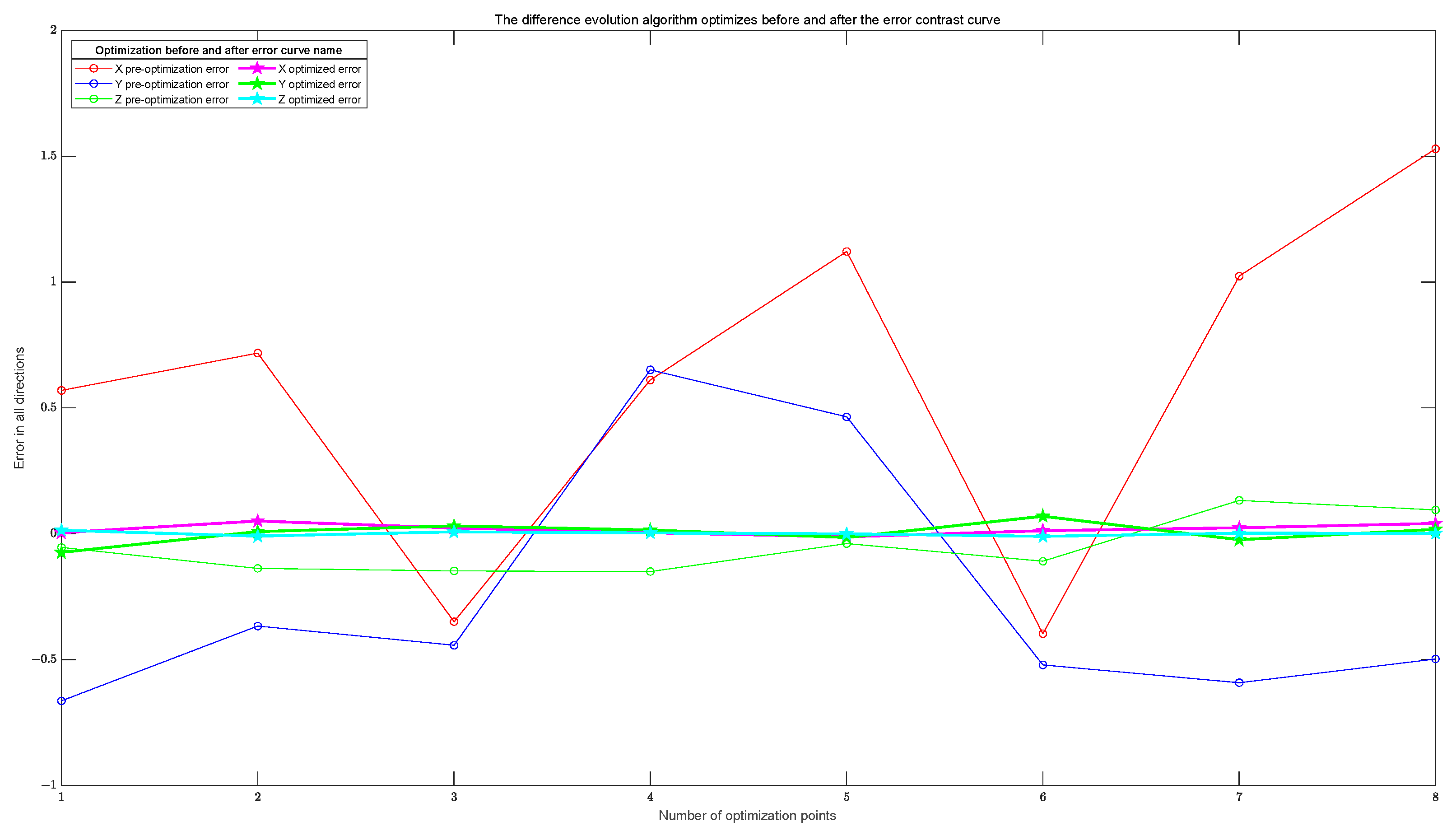
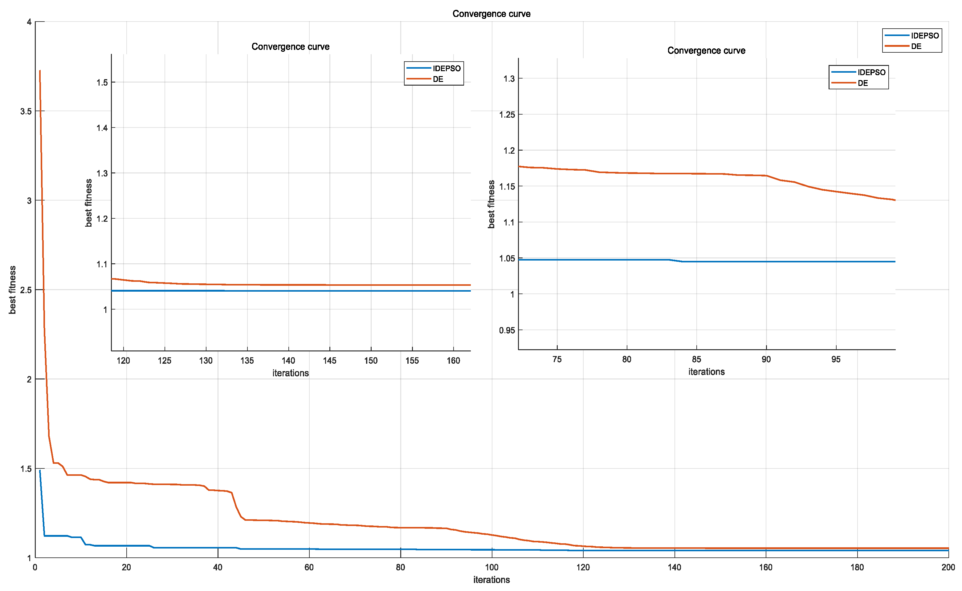
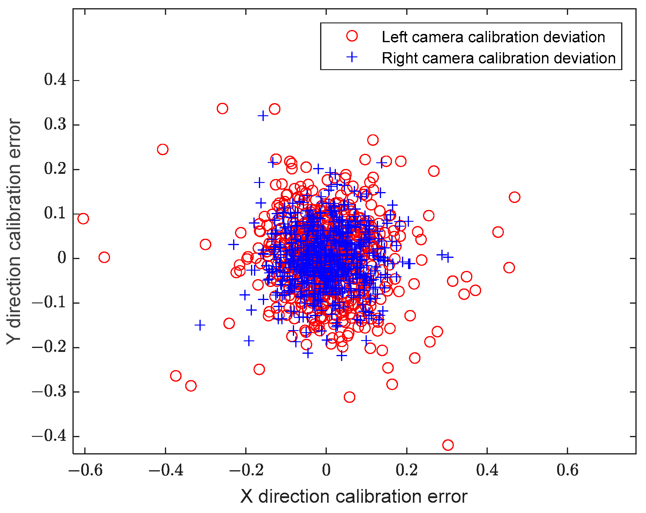
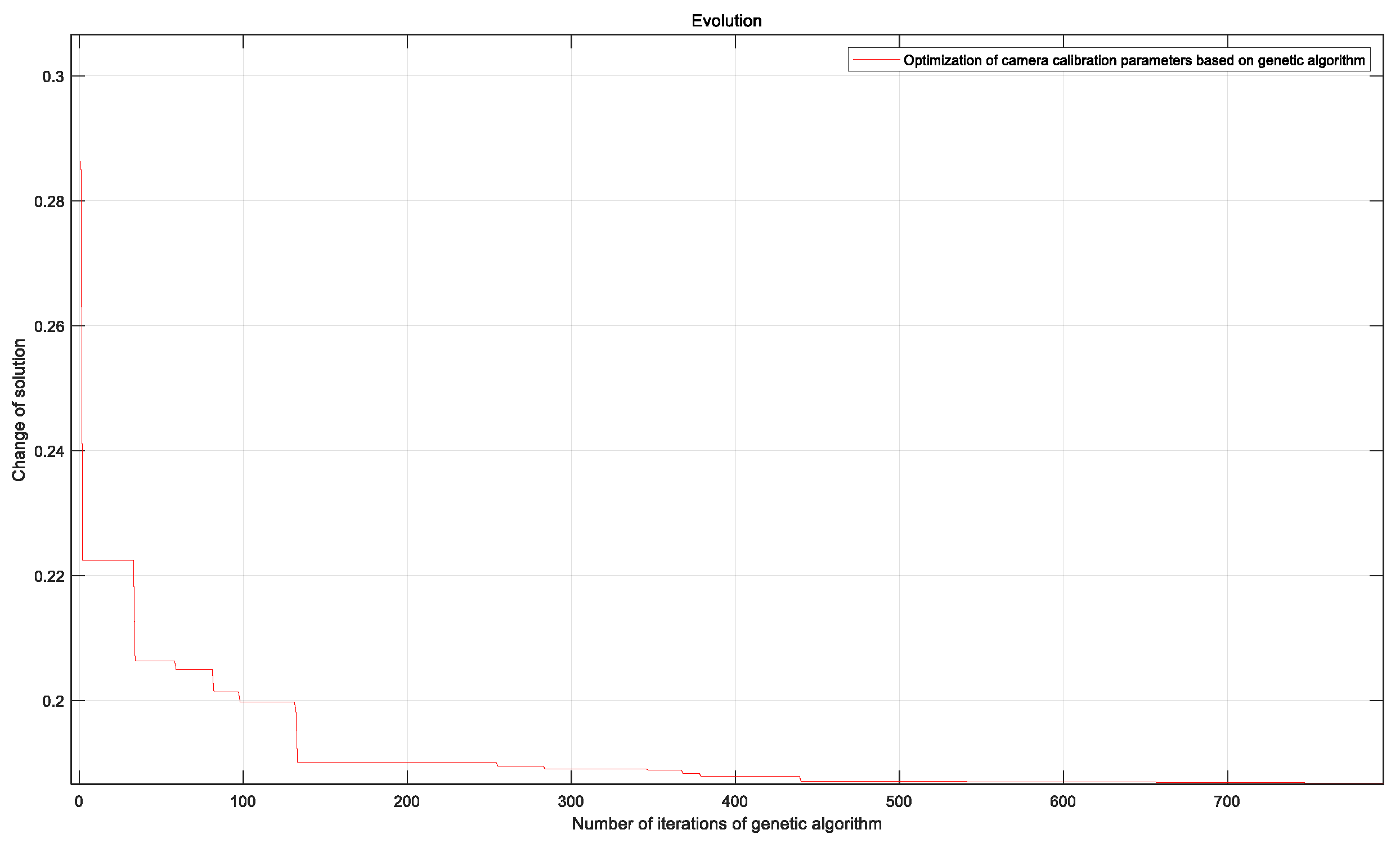
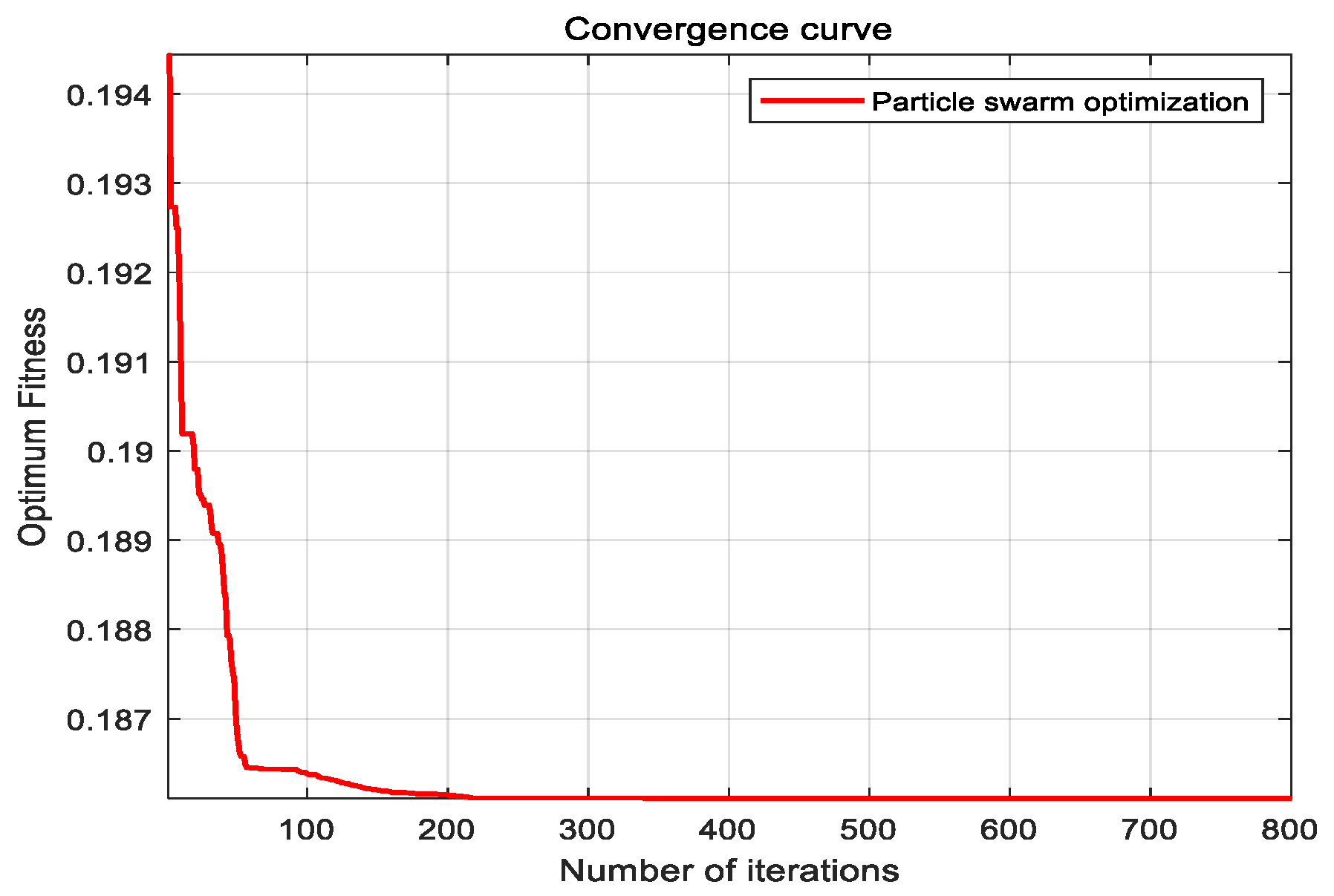
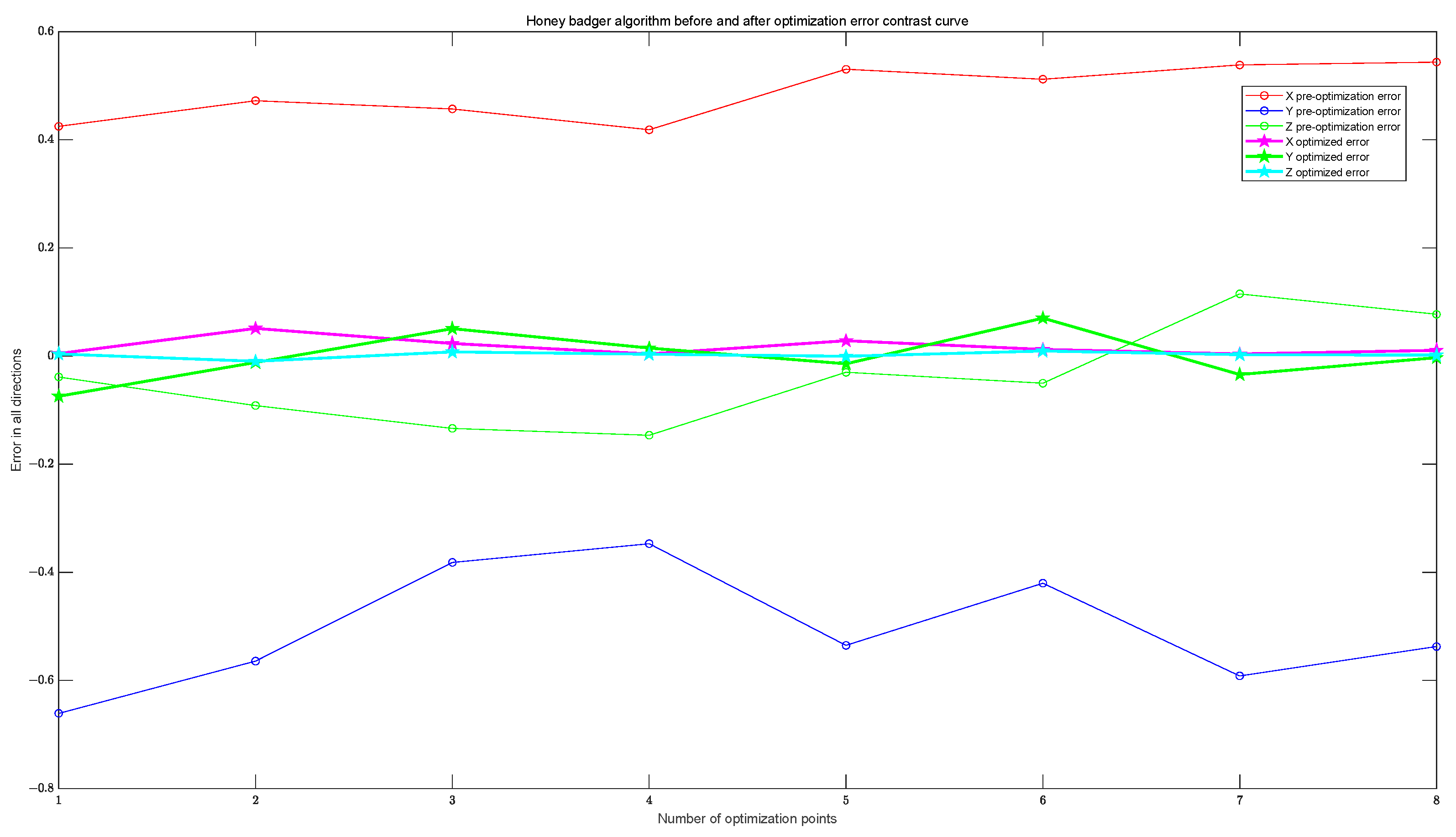
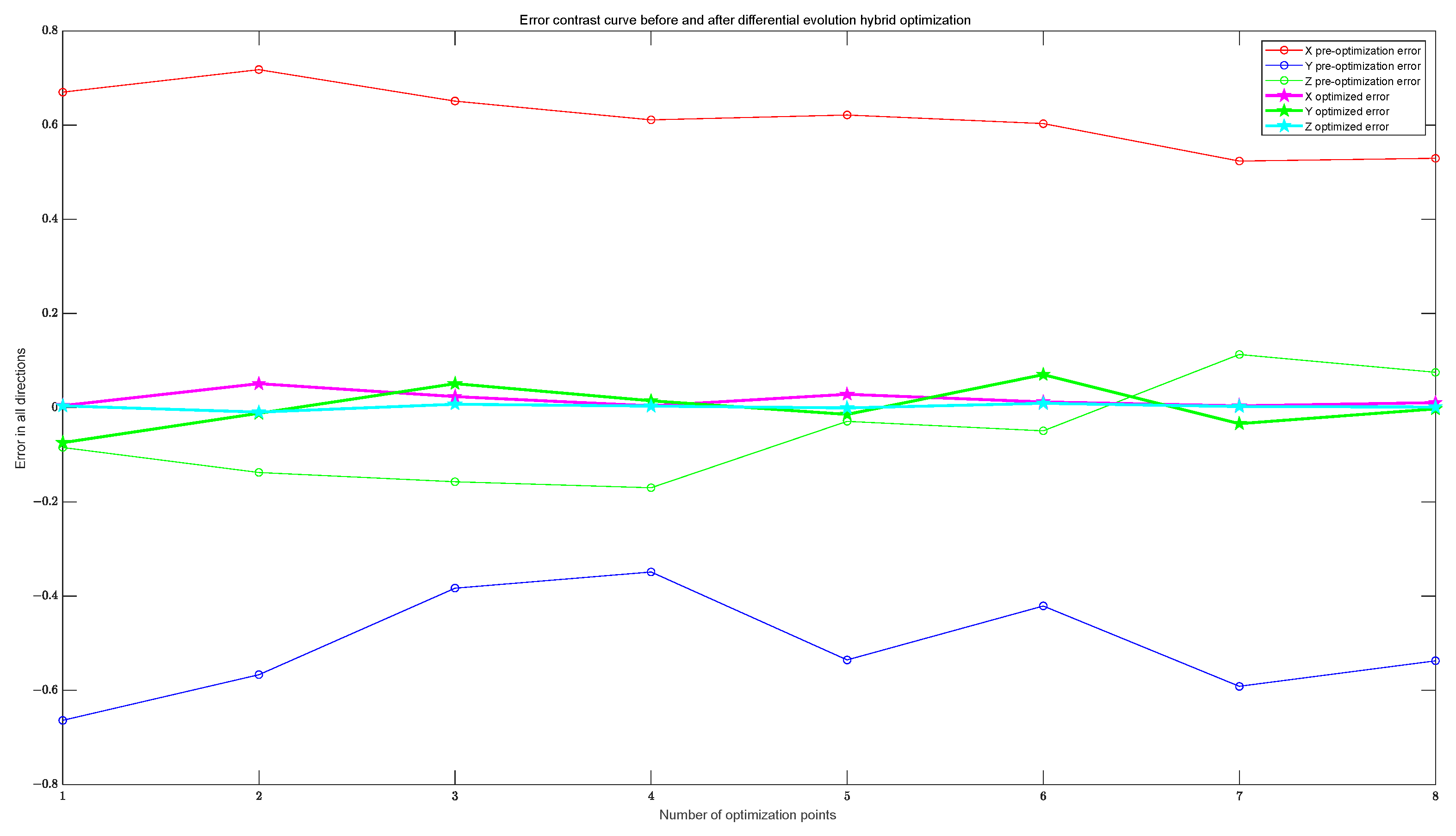
5.2. Results and Analysis

A binocular camera is used to take multiple photos, which are shown in Figure 10:

In the camera calibration experiments, the calibration board underwent movement within the field of view of the camera, assuming different positions and angles. This allowed for the capture of multiple sets of detection images for the purpose of calibration. Due to the continuous movement of the calibration board, image blurring may occur during image acquisition, which in turn can affect the accuracy of subsequent corner detection. Therefore, high-quality, non-blurred images were selected from the collected calibration data for the calibration experiments. The process of binocular calibration and corner detection is illustrated in Figure 11.

The method for camera calibration detailed earlier was applied to derive parameter matrices $M_1$ and $M_2$ for the left and right cameras. Correspondingly, matrices $D_1$ and $D_2$ representing the distortion parameters for the cameras were acquired. A summary of the findings can be found in

Table 1. The calibration parameter matrix for the left and right cameras.

Camera Parameter Matrix	Distortion Parameter Matrix
$M_1=\left[\begin{array}{ccc}5035.73040& 0& 533.22766\\ 0& 5036.77009& 978.66847\\ 0& 0& 1\end{array}\right]$	$D_1=[-0.08209,1.58242,-0.00166,-0.00032,10.23747]$
$M_2=\left[\begin{array}{ccc}5018.27022& 0& 516.49581\\ 0& 5017.48057& 905.64914\\ 0& 0& 1\end{array}\right]$	$D_2=[-0.05939,0.48486,-0.00168,-0.00026,38.70554]$

, with all data rounded to five decimal places.

During this experiment, 15 sets of calibration board images were utilized. The intrinsic and extrinsic parameters of the camera, along with the distortion parameters obtained from the calibration process, were employed to project the corners of the calibration board onto the imaging plane. The calibration error was subsequently evaluated by comparing the pixel coordinates of these points with their actual coordinates on the calibration board. The tabulated results of the calibration errors are documented in

Table 2. Calibration average error table.

Label	Average Error (Pixel)	Label	Average Error (Pixel)	Label	Average Error (Pixel)
1	0.172649	6	0.138521	11	0.189421
2	0.157981	7	0.137715	12	0.212029
3	0.081947	8	0.141941	13	0.118467
4	0.105237	9	0.166069	14	0.193648
5	0.160528	10	0.233748	15	0.189421

.

As shown in Table 2, the overall average calibration error falls within a range of 0.25 pixels.

Figure 12 illustrates the projection of the calibration board’s corner coordinates onto the camera coordinate plane using the camera’s intrinsic and extrinsic parameters derived from reverse projection. Discrepancies between these projected coordinates and the actual corner coordinates in the original image were computed in both the x and y directions. The deviations, quantified in pixels, are denoted by red “o” for the calibration disparities of the left camera and blue “+” for those of the right camera.

After the calibration of both the left and right cameras, the stereo vision calibration can be conducted. The calibration outcomes for the binocular vision system are displayed in

Table 3. Binocular camera calibration results.

Rotation Matrix	Translation Vector
$R=\left[\begin{array}{ccc}-0.99993098& 0.0004564127& -0.011711541\\ -0.00057125383& -0.99995023& 0.0098654972\\ -0.011706779& 0.0098716523& 0.99988127\end{array}\right]$	$T=\left[\begin{array}{ccc}-15.728618& 0.081634976& -0.082594357\end{array}\right]$

.

The rotation matrix and translation matrix for stereo calibration, presented in Table 3, indicate that the rotation matrix bears a striking resemblance to the identity matrix. This similarity can be attributed to the meticulous efforts employed during the setup of the left and right cameras to achieve and maintain their equilibrium.

Following the procedure outlined in the preceding section, the MATLAB implementation of the optimization algorithm program utilized 10 sets of calibration images and experimented with maximum iteration numbers of 200, 400, 600, 800, and 1000. In order to evaluate the calibration performance of the algorithm proposed in this chapter, assessments were carried out employing the genetic algorithm, particle swarm algorithm, honey badger algorithm, and improved differential particle swarm algorithm. The evaluation criteria involved nine parameters, $f_x,f_y,c_x,c_y,k_1,k_2,k_3,p_1,p_2$, and their performance was compared, as presented in

Table 4. Table of the optimization results of the four optimization algorithms for the nine calibration parameters.

Argument	GA	PSO	HBA	IDEPSO	DE
$f_x$	1156.7861	1154.4027	1156.4027	1157.8783	1157.4027
$f_y$	1154.2004	1155.0684	1155.0685	1153.6961	1152.0685
$c_x$	662.7546	660.9385	660.9385	663.02028	662.9385
$c_y$	387.9115	389.3181	389.1970	387.9177	387.8497
$k_1$	−0.2451	−0.26817	−0.26614	−0.245762	−0.245485
$k_2$	−0.044766	−0.06452	−0.06452	−0.044699	−0.044525
$k_3$	−0.00049006	−0.000713	−0.000313	−0.0004727	−0.0005139
$p_1$	5.6293 × 10−5	4.1408 × 10−5	8.1408 × 10−5	4.5905 × 10−5	6.1408 × 10−5
$p_2$	0.045762	0.041302	0.045302	0.045686	0.0456797

.

Based on the findings displayed in Table 4, the camera parameter calibration performed in this investigation meticulously accounted for both radial and tangential distortions. As a result, the influence of distortion and lens aberrations on the measurement outcomes during the camera calibration process was significantly mitigated. To conduct a more comprehensive analysis of the optimization test results, the positional deviations were assessed using the error range and root-mean-square error (RMSE) as indicators of accuracy. The calculation formulas for these two evaluation criteria are provided below:

$$Er(k)=\sqrt{{\left(\widehat{X}(k)-X(k)\right)}^2}\hspace{1em}\hspace{1em}k=1,2,\cdots ,N$$

(58)

$$RMSE=\sqrt{\frac{1}{N}{\displaystyle \sum _{i=1}^N{(\widehat{X}(k)-X(k))}^2}}$$

(59)

The root-mean-square errors for position in each direction calibrated by the four optimization algorithms are presented in

Table 5. Comparison of the four optimization algorithms.

RMSE	X	Y	Z
GA	0.6189	0.5162	0.1124
PSO	0.4895	0.5137	0.0947
HBA	0.3201	0.5150	0.0657
IDEPSO	0.1690	0.3780	0.0638
DE	0.8758	0.5138	0.1151

.

Result 1: The fitness curve for the optimization using genetic algorithm is shown in Figure 13, with a maximum iteration number of 455. The fitness value decreases in a stepwise manner as the iteration number increases and finally reaches zero after 455 iterations. The solution stabilizes thereafter and remains consistent.

Based on Figure 13 and Figure 14, it can be observed that the optimization of calibration parameters using genetic algorithm resulted in significant improvement in the corresponding coordinate errors. The error in the x-coordinate was reduced from approximately 0.3 to within 0.05 after optimization, while the error in the y-coordinate improved from around −0.5 to within ±0.07. The error in the z-coordinate was within 0.1 before parameter optimization.

Result 2: The fitness curve for the optimization using particle swarm algorithm is depicted in Figure 15. The algorithm terminated after 225 iterations, and the fitness value exhibited a stepwise decrease with the increase in iteration count. After 225 iterations, the solution approached zero and stabilized.

The error in the coordinates of the corresponding points before and after optimization can be obtained from Figure 16. Prior to optimizing the calibration parameters, the error in the x-direction of the corresponding points was approximately within 0.27, the y-direction error was within −0.65, and the z-direction error was within −0.12. After optimization using the particle swarm algorithm, the x-direction error was within 0.05, the y-direction error fluctuated within ±0.07, and the z-direction error was within 0.07. It can be noted that the particle swarm optimization method demonstrated a relatively better improvement in the y-direction error.

Result 3: The fitness curve after optimizing using the honey badger algorithm is depicted in Figure 17. The algorithm terminated after 122 iterations, and the fitness value progressively decreased in a stepped manner with increasing iteration count. After 122 iterations, the solution approached zero and reached stability. Based on the convergence of the curve, it is evident that this algorithm exhibits noticeably faster convergence speed and requires fewer iterations compared to the previous two optimization algorithms.

Figure 18 shows the coordinate error curve before and after optimizing the camera calibration parameters using the honey badger algorithm. Based on the error curve, it can be concluded that the honey badger optimization algorithm reduced the error in the x-direction from 0.56 before optimization to within 0.05 after optimization. Furthermore, the algorithm decreased the error in the y-direction from −0.66 to within 0.07 and in the z-direction from −0.14 to within ±0.06. These results indicate that the algorithm greatly improves the error.

Result 4: The fitness curve after optimizing using the improved differential evolution particle swarm algorithm is shown in the Figure 19 and Figure 20. It can be observed that the curve depicted fluctuations throughout the first 150 iterations before stabilizing around iteration 400, at which point the calibration optimization results attain stability.

As shown in the above figure, the error curve of the experimental data point coordinates before and after optimizing the camera calibration parameters using the mixed optimization algorithm based on improved differential evolution and particle swarm can be observed. It is apparent that prior to using the mixed optimization algorithm, the error in the x-direction was approximately 0.7, which was reduced to within 0.005 after optimization. Additionally, the error in the y-direction decreased from −0.66 to around −0.07, and the error in the z-direction decreased from −0.17 to near 0. These experimental results indicate that although the convergence speed and iteration count of this algorithm are not the fastest compared to several other optimization algorithms, the optimized parameter results are favorable. Therefore, the mixed optimization algorithm based on improved differential evolution and particle swarm demonstrates the best optimization effect with the lowest error.

Result 5: The fitness curve following DE optimization, as shown in Figure 21, concluded at iteration 335, demonstrating a stepwise decrease in fitness as the number of iterations increased.

As evidenced by Figure 21 and Figure 22, notable changes in the corresponding coordinate errors are observed before and after optimization using the differential evolution algorithm. Specifically, errors in the corresponding $x$-coordinate parameters were approximately 1.5 before optimization and reduced to within 0.1 post-optimization. Errors in the corresponding $y$-coordinates were approximately 0.6 before optimization and reduced to within plus or minus 0.1 afterward. For $z$-coordinates, errors were within 0.2 before optimization and reduced to within 0.05 after optimization. It is evident that prior to optimization, error fluctuations were significant, whereas a substantial reduction in errors was observed following optimization.

Upon comparison with the DE algorithm, it is noted that there is not a significant disparity in the fitness curves of the two algorithms. In light of this observation, additional experiments were conducted wherein the fitness curves of both algorithms were juxtaposed. The experiments were conducted over 200 iterations, yielding the following results (Figure 23):

Specific indicators are shown in

Table 6. Performance comparison of algorithm convergence curves.

	DE	IDEPSO
Fitness value	1.04488	1.04068
Number of iterations when stabilizing	128	84

:

The examination of the referenced charts reveals that the IDEPSO achieves a more rapid convergence compared to DE. It is observed that the proposed algorithm approaches stability after 84 iterations, exhibiting a stable fitness value of 1.04068, whereas the stability for the DE algorithm is reached after 128 iterations with a fitness value of 1.04488. In the context of mean-square errors (MSE) across various axes, it is evident that post-optimization, the algorithm we introduced demonstrates significantly reduced MSE values on all axes when juxtaposed with the DE algorithm. Furthermore, the enhanced Differential Evolution Particle Swarm Optimization (DEPSO) algorithm yields a mere 0.1690 root-mean-square error in the x-axis, 0.3780 in the y-axis, and 0.0638 in the z-axis. These calibration results undercut the calibration errors associated with the other three optimization calibration methods, substantiating the exemplary performance and high accuracy of our algorithm.

6. Conclusions

This paper first introduces the structure and coordinate system conversion of the photogrammetry system. It then provides a detailed description of commonly used camera calibration methods and investigates distortion models for camera calibration. Based on this research, an optimized method for calibrating cameras is proposed, which utilizes a new algorithm capable of accurately calibrating cameras. In this algorithm, iterations are incorporated into the mutation and crossover stages of the differential evolution process, and the dynamic adjustment strategy is refined. Introducing the concept of differential evolution ensures the preservation of particle population diversity, enabling the selection of the globally optimal particle at each iteration for the attainment of more precise results. Experimental comparisons among the calibration algorithm proposed in this paper and particle swarm optimization calibration, genetic algorithm optimization, and honey badger algorithm demonstrate its superior performance parameters, smaller calibration errors, and advantageous algorithm performance.

References

- Han, C.Z.; Zhu, H.Y. Multi-Source Information Fusion; Tsinghua University Press: Beijing, China, 2010; pp. 1–18. [Google Scholar]
- Ma, T.L.; Wang, X.M. Variational Bayesian STCKF for systems with uncertain model errors. Control Decis. 2016, 31, 2255–2260. [Google Scholar]
- Feng, X.X.; Chi, L.J.; Wang, Q. An improved generalized labeled multi-Bernoulli filter for maneuvering extended target tracking. Control Decis. 2019, 43, 2143–2149. [Google Scholar]
- Rui, Z.; Yu, F.; Bin, D.; Jiang, Z. Multi-UAV cooperative target tracking with bounded noise for connectivity preservation. Front. Inf. Technol. Electron. Eng. 2020, 21, 1413–1534. [Google Scholar]
- Sarkka, S. Recursive Noise Adaptive Kalman Filtering by Variational Bayesian Approximations. IEEE Trans. Autom. Control 2009, 54, 596–600. [Google Scholar] [CrossRef]
- Xu, H.; Xie, W.C.; Yuan, H.D. Maneuvering Target Tracking Algorithm Based on the Adaptive Augmented State Interacting Multiple Model. J. Electron. Inf. Technol. 2020, 42, 2749–2757. [Google Scholar]
- Liang, Y.; Jia, Y.G.; Pan, Q. Parameter Identification in Switching Multiple Model Estimation and Adaptive Interacting Multiple Model Estimator. Control Theory Appl. 2001, 18, 653–656. [Google Scholar]
- Jiang, W.; Wang, Z. Calibration of visual model for space manipulator with a hybrid LM–GA algorithm. Mech. Syst. Signal Process. 2016, 66–67, 399–409. [Google Scholar] [CrossRef]
- Liu, J.Y.; Wang, C.P.; Wang, W. SMC-CMeMBer filter based on pairwise Markov chains. Syst. Eng. Electron. 2019, 41, 1686–1691. [Google Scholar]
- Huang, D.; Leung, H. Maximum Likelihood State Estimation of Semi-Markovian Switching System in Non-Gaussian Measurement Noise. IEEE Trans. Aerosp. Electron. Syst. 2010, 46, 133–146. [Google Scholar] [CrossRef]
- Wang, Z.; Shen, X.; Zhu, Y. Ellipsoidal Fusion Estimation for Multisensor Dynamic Systems with Bounded Noises. IEEE Trans. Autom. Control 2019, 64, 4725–4732. [Google Scholar] [CrossRef]
- Sun, W.; Zhao, X.Y. Maneuvering target tracking with the extended set-membership filter and information geometry. J. Terahertz Sci. Electron. Inf. Technol. 2018, 16, 786–790. [Google Scholar]
- Mahler, R. General Bayes filtering of quantized measurements. In Proceedings of the 14th International Conference on Information Fusion, Chicago, IL, USA, 5–8 July 2011; pp. 1–6. [Google Scholar]
- Ristic, B. Bayesian Estimation with Imprecise Likelihoods: Random Set Approach. IEEE Signal Process. Lett. 2011, 18, 395–398. [Google Scholar] [CrossRef]
- Hanebeck, U.D.; Horn, J. Fusing information simultaneously corrupted by uncertainties with known bounds and random noise with known distribution. Inf. Fusion 2000, 1, 55–63. [Google Scholar] [CrossRef]
- Duan, Z.; Jilkov, V.P.; Li, X.R. State estimation with quantized measurements: Approximate MMSE approach. In Proceedings of the 11th International Conference on Information Fusion, Cologne, Germany, 30 June–3 July 2008; pp. 1–6. [Google Scholar]
- Miranda, E. A survey of the theory of coherent lower previsions. Int. J. Approx. Reason. 2008, 48, 628–658. [Google Scholar] [CrossRef]
- Benavoli, A.; Zaffalon, M.; Miranda, E. Robust Filtering Through Coherent Lower Previsions. IEEE Trans. Autom. Control 2011, 56, 1567–1581. [Google Scholar] [CrossRef]
- Peter, W. Statistical Reasoning with Imprecise Probabilities; Chapman and Hall: New York, NY, USA, 1991; pp. 1–35. [Google Scholar]
- Noack, B.; Klumpp, V.; Hanebeck, U.D. State estimation with sets of densities considering stochastic and systematic errors. In Proceedings of the 12th International Conference on Information Fusion, Seattle, WA, USA, 6–9 July 2009; pp. 1–6. [Google Scholar]
- Klumpp, V.; Noack, B.; Baum, M. Combined set-theoretic and stochastic estimation: A comparison of the SSI and the CS filter. In Proceedings of the 13th International Conference on Information Fusion, Edinburgh, UK, 26–29 July 2010; pp. 1–7. [Google Scholar]
- Gning, A.; Mihaylova, L.; Abdallah, F. Mixture of uniform probability density functions for nonlinear state estimation using interval analysis. In Proceedings of the 13th International Conference on Information Fusion, Edinburgh, UK, 26–29 July 2010; pp. 1–6. [Google Scholar]
- Henningsson, T. Recursive state estimation for linear systems with mixed stochastic and set-bounded disturbances. In Proceedings of the 47th IEEE Conference on Decision and Control, Cancun, Mexico, 9–11 December 2008; pp. 1–6. [Google Scholar]
- Jiang, T.; Qian, F.C.; Yang, H.Z. A New Combined Filtering Algorithm for Systems with Dual Uncertainties. Acta Autom. Sin. 2016, 42, 535–544. [Google Scholar]
- Matthew, J.B. Variational Algorithms for Approximate Bayesian Inference; University of Cambridge: London, UK, 1998; pp. 20–32. [Google Scholar]