Vibration Characteristics of a Functionally Graded Viscoelastic Fluid-Conveying Pipe with Initial Geometric Defects under Thermal–Magnetic Coupling Fields

Abstract

In this study, the Kevin–Voigt viscoelastic constitutive relationship is used to investigate the vibration characteristics and stability of a functionally graded viscoelastic(FGV) fluid-conveying pipe with initial geometric defects under thermal–magnetic coupling fields. First, the nonlinear dimensionless differential equations of motion are derived by applying Timoshenko beam theory. Second, by solving the equilibrium position of the system, the nonlinear term in the differential equations of motion is approximated as the sum of the longitudinal displacement at the current time and longitudinal displacement relative to the position, and the equations are linearized. Third, these equations are discretized using the Galerkin method and are numerically solved under simply supported conditions. Finally, the effects of dimensionless temperature field parameters, dimensionless magnetic field parameters, thermal–magnetic coupling, initial geometric defect types, and the power-law exponent on the complex frequency of the pipe are examined. Results show that increasing the magnetic field intensity enhances the critical velocity of first-order mode instability, whereas a heightened temperature variation reduces the critical velocity of first-order diverge instability. Under thermal–magnetic fields, when the magnetic field intensity and temperature difference are simultaneously increased, their effects on the complex frequency can partially offset each other. Increasing the initial geometric defect amplitude increases the imaginary parts of the complex frequencies; however, for different types of initial geometric defect tubes, it exhibits the most distinct influence only on a certain order.

1. Introduction

Pipes play a vital role in various industries such as the hydropower, petroleum, and nuclear power sectors, serving as a ubiquitous element. Any significant vibration or rupture of these pipes can have severe consequences, ranging from minor issues such as liquid or gas leakage to more catastrophic events such as explosions or fires. Consequently, the study of pipe behavior has consistently garnered the attention of scholars [1,2,3,4,5,6,7].

Functionally graded materials (FGMs) represent specialized materials comprising two or more different materials with continuously spatially varying properties. They have proven effective in enhancing the fracture toughness of brittle ceramics by introducing plastic-deformed metal phases [8]. In recent years, FGMs have been extensively applied in the design of fluid-conveying pipes. Imek analyzed the frequencies of FGM beams under different boundary conditions [9]. Fallah and Aghdam [10] introduced an analytical expression for an FGM beam resting on an inelastic foundation, assessed the validity of the proposed variational method for model calculation, and analyzed the factors affecting frequencies. Shen et al. [11] designed a new FGM shell model to improve the stability of shell systems artificially. Utilizing the differential transformation method, Wattanasakulpong and Ungbhakorn [12] investigated the vibration characteristics and vibration response of an FGM beam, exploring the effects of factors such as material properties and porosity on frequency. Zhu et al. [13] scrutinized the vibration characteristics of an FGM fluid-conveying pipe with non-uniform porosity on a nonlinear elastic foundation, examining the effects of pipe geometry and porosity on pipe vibration characteristics. Khodabakhsh et al. [14] researched the vibration problems in an FGM fluid-conveying pipe and proposed, for the first time, the effects of moment of inertia and shear deformation on vibration. Xu et al. [15] studied the vibration responses and dynamic characteristics of functionally graded cylinders and imperfect microbeams under dynamic harmonic loads. Rezaiee-Pajand and Masoodi [16,17] examined conical beams and columns with a functional classification of the cross-section, verified the effectiveness of the stiffness matrix, and provided an effective calculation unit for the study of functionally graded material shells. Masoodi and Ghandehari [18] studied the dynamic characteristics of functionally graded single-wall carbon nanocoupled curved beams and analyzed the effects of factors such as curvature and interface stiffness on the vibration characteristics of the system.

Viscoelastic materials are commonly employed to mitigate vibrations in fluid-conveying pipes, owing to their ability to dampen vibrations resulting from energy dissipation. Rajidi et al. [19] studied the dynamic characteristics of each order of viscoelastic sandwich pipes, analyzing many factors that influence the damping frequency. Amirinezhad et al. [20] studied wave propagation in functionally graded viscoelastic (FGV) plates using the Zener model, investigating the effect of power-law exponent and geometric parameters of the plates on wave velocity. Deng et al. [21,22] proposed a new method to study the complex frequency of viscoelastic multi-transfunctional gradient macropipes and micropipes, exploring the influence of multiple factors on the system frequency. Hosseini-Hashemi et al. [23] delved into the vibration frequency of an FGV cylindrical plate based on the Zener model and discussed the factors affecting the dynamic characteristics of the model. Based on Timoshenko beam theory, Pinnola et al. [24] derived the differential equations of motion of fractional derivative viscoelastic microbeams and analyzed the effects of nonlocal parameters and viscoelasticity on the vibration response of the system. Fu et al. [25] studied the vibration characteristics of a viscoelastic axially functionally graded material pipe, wherein the fluid is considered to undergo a pulsating internal flow, and analyzed the influence of material characteristics on the nonlinear dynamic characteristics of the system.

Owing to evolving engineering requirements and rapid advancement of pipe technology, fluid-conveying pipes have been installed in many complex physical environments. Ensuring the performance of fluid-conveying pipes under complex and variable working environments necessitates careful consideration of the influence of temperature variation and magnetic field on the stability of the pipes at the initial stages of pipe design. Further, maximizing the stability of the fluid-conveying pipe system should be achieved through the design of relevant parameters [26,27,28]. Akintoye and Oyediran [26] investigated the dynamic characteristics of fluid-conveying pipes under different boundary conditions, exploring the effects of temperature variations and initial curvature on the model dynamics. Building upon the principles of high-order continuous mechanics, Ma and Mu [29] investigated the stability of pure elastic flow microtubules within a thermal–magnetic coupling field. Meanwhile, using a multiscale method, Lu et al. [30] delved into the mechanical model of a magnetoelastic beam subjected to a periodic magnetic field. They comprehensively analyzed the T², steady-state, and limit cycle responses of the system. Zhou et al. [31] studied the static properties of soft magnetic beam plates under the influence of magnetic fields, highlighting the direct proportionality between the bending strength of magnetic elasticity and the bevel angle of the beam. Employing the incremental harmonic balance method, Wu et al. [32] probed the dynamic behavior of a beam exposed to thermal–magnetic effects, investigating the vibration characteristics of the model across different oscillation frequencies. Hosseini and Sadeghi-Goughari [33] applied the differential transformation method to analyze the influence of magnetic field parameters on the vibration of carbon flow nanotubes. Their study included an analysis of the effects of nonlocal and magnetic field parameters on the natural frequency of the system. Pisarski et al. [34] conducted an in-depth investigation of the dynamic characteristics of an electromagnetically driven cantilevered fluid-conveying pipe. Finally, Zhong et al. [35] studied the variations in FGM fluid-conveying pipes on an elastic foundation within a uniformly distributed temperature field, providing insights into the effects of factors such as different power-law distributions and elastic foundation stiffnesses on the system dynamic characteristics. Chen et al. [36] derived and solved the nonlinear vibration equation of FG-CNTRC in thermal environments and also investigated the vibration frequency and influencing factors of the system.

Most previous studies have primarily focused on ideally straight or curved pipes. However, in practical engineering applications, owing to irregular installations or variations in terrain, pipes often exhibit an inherent initial geometric curvature, commonly known as initial geometric defects. Nevertheless, research on fluid-conveying pipes with such characteristics has been limited. To address this gap, Li and Qiao [37] studied the static behavior of beams featuring an initial curvature, analyzing the factors influencing the buckling behavior of the system under different boundary conditions. Ding et al. [38] studied the dynamic characteristics of functionally graded pipes with initial geometric defects. Further, they analyzed the influence of temperature variation and other factors on the nonlinear dynamic characteristics. Liu et al. [39] delved into the vibration characteristics of FGM nanotubes with initial geometric defects, exploring the effects of size parameters and defect types on the vibration characteristic of the system. Meanwhile, Zhu et al. [40] studied the nonlinear vibration of an FGM fluid-conveying pipe that exhibited defects and pores, determining the natural frequencies and factors influencing the model. Using the nonlocal continuum theory, Farshidianfar and Soltani [41] studied the dynamic behavior of single carbon nanotubes with initial geometric defects on a Pasternak elastic foundation.

Despite these valuable contributions, most studies thus far have considered pure elastic functionally graded pipes, and research on viscoelastic FGMs has focused on ideal straight or bent pipes. In this study, the integer-order Kelvin–Voigt model is used to model the pipe material. Assuming that the elastic and viscous terms of the material are functionally graded, the vibration characteristics of an FGV fluid-conveying pipe with initial geometric defects under thermal–magnetic coupling fields are studied for the first time. To this end, the authors derive the nonlinear governing differential equation of the FGV fluid-conveying pipe system with initial geometric defects within the thermal–magnetic coupling field, utilizing the Hamilton principle. Subsequently, the equation is solved using the Galerkin method. Finally, this study delves into the effects of dimensionless temperature parameters, dimensionless magnetic parameters, thermal–magnetic coupling, defect amplitudes, and power-law exponents on the vibration characteristics of the fluid-conveying pipe. Appendix A depicts the flowchart of the analysis performed in this study.

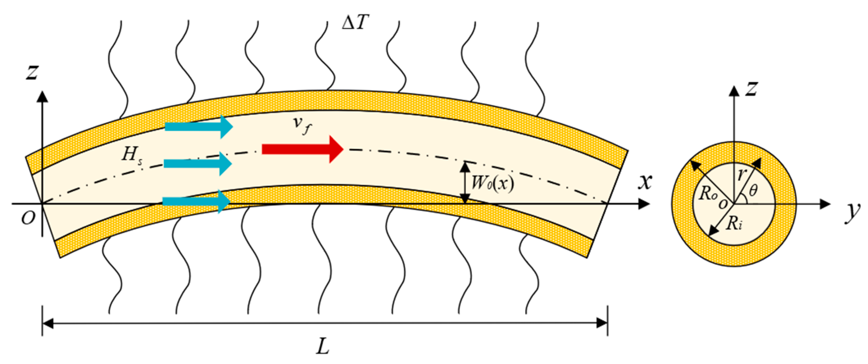
2. Mathematical Model

Figure 1 illustrates an FGV fluid-conveying pipe with initial geometric defects $w_0\left(x\right)$ operating within a thermal–magnetic coupling field. The pipe is characterized by its inner radius $R_i$, its outer radius $R_o$, its length L, the flow velocity represented by $v_f$, the magnetic field strength denoted as H_s, and the temperature variation noted as $\Delta T$.

The elastic modulus $E\left(r\right)$, density $\rho \left(r\right)$, viscosity coefficient $\eta \left(r\right)$, shear modulus $G\left(r\right)$, and thermal expansion coefficient $\alpha \left(r\right)$ of the FGV fluid-conveying pipe obey the following variation functions [42]:

$$\begin{array}{l}E\left(r\right)=E_o+\left(E_i-E_o\right){\left(\frac{R_o-r}{R_o-R_i}\right)}^k,\\ \rho \left(r\right)={\rho }_o+\left({\rho }_i-{\rho }_o\right){\left(\frac{R_o-r}{R_o-R_i}\right)}^k,\\ \eta \left(r\right)={\eta }_o+\left({\eta }_i-{\eta }_o\right){\left(\frac{R_o-r}{R_o-R_i}\right)}^k,\\ G\left(r\right)=G_o+\left(G_i-G_o\right){\left(\frac{R_o-r}{R_o-R_i}\right)}^k,\\ \alpha \left(r\right)={\alpha }_o+\left({\alpha }_i-{\alpha }_o\right){\left(\frac{R_o-r}{R_o-R_i}\right)}^k,\end{array}$$

(1)

where the subscript o signifies the outer surface, i represents the inner surface, and k denotes the power-law exponent.

Based on Timoshenko beam theory, the displacement component at any point within the FGV fluid-conveying pipe can be expressed as

$$\begin{gathered} u_x(x,z,t)=u(x,t)-z\phi (x,t), \\ {w}_z(x,z,t)=w(x,t)+w_0(x), \end{gathered}$$

(2)

where $u_x$ and $w_z$ represent the displacements of any point within the fluid-conveying pipe in the x and z directions, respectively; u and w represent the displacements of any point along the pipe axis in the x and z directions, respectively; and $\phi$ represents the cross-sectional angle of the pipe.

The geometric equation for the model can be expressed as follows:

$${\epsilon }_x=\frac{\partial u}{\partial x}-z\frac{\partial \phi }{\partial x}+\frac{\partial w_0}{\partial x}\frac{\partial w}{\partial x}+\frac{1}{2}{\left(\frac{\partial w}{\partial x}\right)}^2,$$

(3)

$${\gamma }_{xz}=\frac{\partial w}{\partial x}-\phi ,$$

(4)

where $\frac{\partial w_0}{\partial x}\frac{\partial w}{\partial x}$ represents the strain resulting from the initial geometric curvature of the pipe [43] and ${\epsilon }_x$ and ${\gamma }_{xz}$ denote the axial and shear strains at any given point, respectively.

The constitutive relationship of the system is modeled using the Kevin–Voigt model as follows:

$${\sigma }_x=\left[E\left(r\right)+\eta \left(r\right)\frac{\partial }{\partial t}\right]{\epsilon }_x=\left[E\left(r\right)+\eta \left(r\right)\frac{\partial }{\partial t}\right]\left[\frac{\partial u}{\partial x}-z\frac{\partial \phi }{\partial x}+\frac{\partial w_0}{\partial x}\frac{\partial w}{\partial x}+\frac{1}{2}{\left(\frac{\partial w}{\partial x}\right)}^2\right],$$

(5)

$${\tau }_{xz}=k_{s}G\left(r\right){\gamma }_{xz}=k_{s}G(r)(\frac{\partial w}{\partial x}-\phi ),$$

(6)

where k_s represents the cross-sectional form factor of the Timoshenko pipe [44]

$$k_s=\frac{6\left(1+\mu \right){[1+{\left(R_i/R_o\right)}^2]}^2}{\left(7+6\mu \right){[1+{\left(R_i/R_o\right)}^2]}^2+\left(20+12\mu \right){\left(R_i/R_o\right)}^2},$$

(7)

where μ is Poisson’s ratio.

Using Equations (5) and (6), the axial force $N_x$, bending moment $M_y$, and shear force $Q_z$ acting on the cross-section of the pipe can be expressed as follows:

$$\begin{array}{l}{N}_x={\displaystyle {\int }_{A_p}{\sigma }_x\mathrm{d}{A}_p}={\displaystyle {\int }_{A_p}E\left(r\right)\left(1+\eta \frac{\partial }{\partial t}\right)\left[\frac{\partial u}{\partial x}-z\frac{\partial \phi }{\partial x}+\frac{\partial w_0}{\partial x}\frac{\partial w}{\partial x}+\frac{1}{2}{\left(\frac{\partial w}{\partial x}\right)}^2\right]\mathrm{d}{A}_p}\\ =\left(A_{11}+E_{11}\frac{\partial }{\partial t}\right)\left[\frac{\partial u}{\partial x}+\frac{\partial w_0}{\partial x}\frac{\partial w}{\partial x}+\frac{1}{2}{\left(\frac{\partial w}{\partial x}\right)}^2\right]-\left(B_{11}+C_{11}\frac{\partial }{\partial t}\right)\frac{\partial \phi }{\partial x},\end{array}$$

(8)

$$\begin{array}{l}{M}_y={\displaystyle {\int }_{A_p}z{\sigma }_x\mathrm{d}{A}_p}={\displaystyle {\int }_{A_p}z\left(E\left(r\right)+\eta \left(r\right)\frac{\partial }{\partial t}\right)\left[\frac{\partial u}{\partial x}-z\frac{\partial \phi }{\partial x}+\frac{\partial w_0}{\partial x}\frac{\partial w}{\partial x}+\frac{1}{2}{\left(\frac{\partial w}{\partial x}\right)}^2\right]\mathrm{d}{A}_p}\\ =\left(B_{11}+C_{11}\frac{\partial }{\partial t}\right)\left[\frac{\partial u}{\partial x}+\frac{\partial w_0}{\partial x}\frac{\partial w}{\partial x}+\frac{1}{2}{\left(\frac{\partial w}{\partial x}\right)}^2\right]-\left(D_{11}+G_{11}\frac{\partial }{\partial t}\right)\frac{\partial \phi }{\partial x},\end{array}$$

(9)

$$Q_z=k_s{\displaystyle {\int }_{A_p}{\tau }_{xz}\mathrm{d}{A}_p}=k_s{\displaystyle {\int }_{A_p}G\left(r\right)\left(\frac{\partial w}{\partial x}-\phi \right)\mathrm{d}{A}_p}=k_s{A}_{22}\left(\frac{\partial w}{\partial x}-\phi \right),$$

(10)

where

$$\begin{gathered} A_p=\pi \left(R_o^2-R_i^2\right) , \\ \left(A_{11}, E_{11}, A_{22}\right)={\displaystyle {\int }_0^{2\pi }{\displaystyle {\int }_{R_i}^{R_o}\left(\frac{E(r)}{1-{\mu }^2}, \frac{\eta (r)}{1-{\mu }^2}, \frac{E(r)}{2\left(1+\mu \right)}\right)}}r\mathrm{d}r\mathrm{d}\theta , \\ \left(B_{11}, C_{11} \right)={\displaystyle {\int }_0^{2\pi }{\displaystyle {\int }_{R_i}^{R_o}\left(\frac{E(r)}{1-{\mu }^2},\frac{\eta (r)}{1-{\mu }^2} \right)}}{r}^2\sin \theta \mathrm{d}r\mathrm{d}\theta , \\ \left(D_{11}, G_{11}\right)={\displaystyle {\int }_0^{2\pi }{\displaystyle {\int }_{R_i}^{R_o}\left(\frac{E(r)}{1-{\mu }^2},\frac{\eta (r)}{1-{\mu }^2} \right)}}{r}^3{\sin }^2\theta \mathrm{d}r\mathrm{d}\theta , \end{gathered}$$

(11)

The variations in the strain energy $U_p$ and kinetic energy $T$ can be expressed as follows:

$$\begin{array}{l}\delta {\displaystyle {\int }_{t_1}^{t_2}{U}_p}\mathrm{d}t={\displaystyle {\int }_{t_1}^{t_2}{\displaystyle {\int }_0^L{\displaystyle {\int }_{A_p}\left({\sigma }_x\delta {\epsilon }_x+{\tau }_{xz}\delta {\gamma }_{xz}\right)}}\mathrm{d}{A}_p\mathrm{d}x}\mathrm{d}t\\ ={\displaystyle {\int }_{t_1}^{t_2}{\displaystyle {\int }_0^L{\displaystyle {\int }_{A_p}\left[{\sigma }_x\delta \left(\frac{\partial u}{\partial x}-z\frac{\partial \phi }{\partial x}+\frac{\partial w_0}{\partial x}\frac{\partial w}{\partial x}+\frac{1}{2}{\left(\frac{\partial w}{\partial x}\right)}^2\right)+{\tau }_{xz}\delta \left(\frac{\partial w}{\partial x}-\phi \right)\right]}}\mathrm{d}{A}_p\mathrm{d}x\mathrm{d}t}\\ ={\displaystyle {\int }_{t_1}^{t_2}{\displaystyle {\int }_0^L\left[N_x\delta \frac{\partial u}{\partial x}-M_y\delta \frac{\partial \phi }{\partial x}+N_x\delta \left(\frac{\partial w_0}{\partial x}\frac{\partial w}{\partial x}\right)+\frac{1}{2}{N}_x\delta {\left(\frac{\partial w}{\partial x}\right)}^2+Q_z\delta \left(\frac{\partial w}{\partial x}-\phi \right)\right]}\mathrm{d}x\mathrm{d}t},\end{array}$$

(12)

$$\begin{array}{l}\delta {\displaystyle {\int }_{t_1}^{t_2}T}\mathrm{d}t={\displaystyle {\int }_{t_1}^{t_2}{\displaystyle {\int }_0^L\left[m_0\frac{\partial u}{\partial t}\delta \frac{\partial u}{\partial t}+m_0\frac{\partial w}{\partial t}\delta \frac{\partial w}{\partial t}+m_{11}\frac{\partial \phi }{\partial t}\delta \frac{\partial \phi }{\partial t}\right]}}\mathrm{d}x\mathrm{d}t\\ +{\displaystyle {\int }_{t_1}^{t_2}{\displaystyle {\int }_0^L{m}_f\left[\begin{array}{l}\left(v_f+v_f\frac{\partial u}{\partial x}+v_f\frac{\partial u}{\partial t}\right)\delta \left(v_f+v_f\frac{\partial u}{\partial x}+v_f\frac{\partial u}{\partial t}\right)+\\ \left(v_f\frac{\partial w}{\partial x}+\frac{\partial w}{\partial \mathrm{t}}\right)\delta \left(v_f\frac{\partial w}{\partial x}+\frac{\partial w}{\partial \mathrm{t}}\right)\end{array}\right]}}\mathrm{d}x\mathrm{d}t\end{array}$$

(13)

where

$$\begin{array}{l}\left(m_0,m_{11}\right)={\displaystyle {\int }_0^{2\pi }{\displaystyle {\int }_{R_i}^{R_o}\rho (r)\left(1, r^2{\sin }^2\theta \right)}} r\mathrm{d}r\mathrm{d}\theta ,\\ m_f={\rho }_f{A}_f,\hspace{1em}{A}_f=\pi R_i^2.\end{array}$$

(14)

Following Maxwell’s relation, the magnetic field energy performed by a magnetic field can be expressed as [31]

$$U_K=\frac{1}{2}\lambda A_p{H}_s^2{\displaystyle {\int }_0^L{\left(\frac{\partial w}{\partial x}\right)}^2\mathrm{d}x},$$

(15)

where $\lambda$ represents the magnetic permeability.

The variation of magnetic field energy $U_K$ can be expressed as

$$\delta {\displaystyle {\int }_{t_1}^{t_2}{U}_K}\mathrm{d}t={\displaystyle {\int }_{t_1}^{t_2}{\displaystyle {\int }_0^L\lambda A_p{H}_s^2\frac{{\partial }^{2}w}{\partial x^2}}\delta w\mathrm{d}x\mathrm{d}t }.$$

(16)

Based on the thermoelastic theory, the strain energy U_T generated owing to temperature variation is expressed as follows:

$$U_T=-\frac{1}{2}{\displaystyle {\int }_0^L{N}_T}{\left(\frac{\partial w}{\partial x}\right)}^2\mathrm{d}x,$$

(17)

$$N_T=\frac{{\left(E\alpha \right)}_{eq}{A}_p}{1-2\mu }\Delta T,$$

(18)

where N_T is the axial force generated by the temperature variation.

$${\left(E\alpha \right)}_{eq}{A}_p={\displaystyle {\int }_{A_p}E(r)\alpha (r)}\mathrm{d}{A}_p={\displaystyle {\int }_0^{2\pi }{\displaystyle {\int }_{R_i}^{R_o}E(r)\alpha (r)r\mathrm{d}r\mathrm{d}}}\theta ,$$

(19)

The variation of the energy of the temperature field is given by

$$\delta {\displaystyle {\int }_{t_1}^{t_2}{U}_T}\mathrm{d}t={\displaystyle {\int }_{t_1}^{t_2}{\displaystyle {\int }_0^L\frac{{\left(E\alpha \right)}_{eq}{A}_p}{1-2\mu }\Delta T\delta {\left(\frac{\partial w}{\partial x}\right)}^2}\mathrm{d}x\mathrm{d}t }.$$

(20)

The Hamiltonian principle is expressed as follows:

$$\delta {\displaystyle {\int }_{t_1}^{t_2}(T-U_p+U_T+U_K)}\mathrm{d}t=0.$$

(21)

Equations (12)–(20) are substituted into Equation (21), and a variational operation is performed to obtain the nonlinear differential equation of motion of the model.

$$\begin{array}{l}(m_0+m_f)\frac{{\partial }^{2}u}{\partial t^2}+2m_f{v}_f\frac{{\partial }^{2}u}{\partial x\partial t}+m_f{v}_f^2\frac{{\partial }^{2}u}{\partial x^2}\\ -\left(A_{11}+E_{11}\frac{\partial }{\partial t}\right)\frac{\partial }{\partial x}\left[\frac{\partial u}{\partial x}+\frac{\partial w_0}{\partial x}\frac{\partial w}{\partial x}+\frac{1}{2}{\left(\frac{\partial w}{\partial x}\right)}^2\right]=0,\end{array}$$

(22)

$$\begin{array}{l}(m_0+m_f)\frac{{\partial }^{2}w}{\partial t^2}+2m_f{v}_f\frac{{\partial }^{2}w}{\partial x\partial t}+m_f{v}_f^2\frac{{\partial }^{2}w}{\partial x^2}+\frac{{\left(E\alpha \right)}_{eq}{A}_p}{1-2\mu }\Delta T\frac{{\partial }^{2}w}{\partial x^2}-\lambda A_p{H}_s^2\frac{{\partial }^{2}w}{\partial x^2}-\\ k_s{A}_{22}\left(\frac{{\partial }^{2}w}{\partial x^2}-\frac{\partial \phi }{\partial x}\right)-\frac{\partial }{\partial x}\left\{\left(A_{11}+E_{11}\frac{\partial }{\partial t}\right)\left[\frac{\partial u}{\partial x}+\frac{\partial w_0}{\partial x}\frac{\partial w}{\partial x}+\frac{1}{2}{\left(\frac{\partial w}{\partial x}\right)}^2\right]\left(\frac{\partial w_0}{\partial x}+\frac{\partial w}{\partial x}\right)\right\}=0,\end{array}$$

(23)

$$m_{11}\frac{{\partial }^2\phi }{\partial t^2}-\left(D_{11}+G_{11}\frac{\partial }{\partial t}\right)\frac{{\partial }^2\phi }{\partial x^2}-k_s{A}_{22}\left(\frac{\partial w}{\partial x}-\phi \right)=0,$$

(24)

with the boundary conditions

$$\left\{m_f{v}_f^2+m_f{v}_f^2\frac{\partial u}{\partial x}+m_f{v}_f\frac{\partial u}{\partial t}-\left(A_{11}+E_{11}\frac{\partial }{\partial t}\right)\left[\frac{\partial u}{\partial x}+\frac{\partial w_0}{\partial x}\frac{\partial w}{\partial x}+\frac{1}{2}{\left(\frac{\partial w}{\partial x}\right)}^2\right]\right\}\delta u{|}_0^L=0,$$

(25)

$$\left\{\begin{array}{l}{m}_f{v}_f^2\frac{\partial w}{\partial x}+m_f{v}_f\frac{\partial w}{\partial t}-k_s{A}_{22}\left(\frac{\partial w}{\partial x}-\phi \right)+\frac{{\left(E\alpha \right)}_{eq}{A}_p\Delta T}{1-2\mu }\frac{\partial w}{\partial x}-\lambda A_p{H}_s^2\frac{\partial w}{\partial x}-\\ \left(\frac{\partial w_0}{\partial x}+\frac{\partial w}{\partial x}\right)\left(A_{11}+E_{11}\frac{\partial }{\partial t}\right)\left[\frac{\partial u}{\partial x}+\frac{\partial w_0}{\partial x}\frac{\partial w}{\partial x}+\frac{1}{2}{\left(\frac{\partial w}{\partial x}\right)}^2\right]\end{array}\right\}\delta w{|}_0^L=0,$$

(26)

$$\left[\left(D_{11}+G_{11}\frac{\partial }{\partial t}\right)\frac{\partial \phi }{\partial x}\right]\delta \phi {|}_0^L=0.$$

(27)

Because the model described in this paper involves a small and limited stretching problem, the vibration of the pipe in the x-axis direction is neglected, i.e.,

$$\frac{\partial \left[\frac{\partial u}{\partial x}+\frac{\partial w_0}{\partial x}\frac{\partial w}{\partial x}+\frac{1}{2}{\left(\frac{\partial w}{\partial x}\right)}^2\right]}{\partial x}=0,$$

(28)

The left and right sides of Equation (28) are integrated twice with respect to x:

$$u=c_1(t)x+c_2(t)-{\displaystyle {\int }_0^x\left[\frac{\partial w_0}{\partial x}\frac{\partial w}{\partial x}+\frac{1}{2}{\left(\frac{\partial w}{\partial x}\right)}^2\right]}\mathrm{d}x,$$

(29)

The boundary conditions of simple support at both ends of the pipe are as follows:

$$\mathrm{At} x=0 \mathrm{and} x=L, u=w=0 \mathrm{and} \frac{{\partial }^{2}w}{\partial x^2}=0.$$

(30)

Combined with the boundary conditions

$$c_1(t)=\frac{1}{L}{\displaystyle {\int }_0^L\left[\frac{\partial w_0}{\partial x}\frac{\partial w}{\partial x}+\frac{1}{2}{\left(\frac{\partial w}{\partial x}\right)}^2\right]}\mathrm{d}x,\hspace{1em}\hspace{1em}{c}_2(t)=0.$$

(31)

By substituting Equation (31) into Equation (29) and taking the derivative, we obtain

$$\frac{\partial u}{\partial x}=\frac{1}{2L}{\displaystyle {\int }_0^L\left[2\frac{\partial w_0}{\partial x}\frac{\partial w}{\partial x}+{\left(\frac{\partial w}{\partial x}\right)}^2\right]}\mathrm{d}x-\frac{\partial w_0}{\partial x}\frac{\partial w}{\partial x}-\frac{1}{2}{\left(\frac{\partial w}{\partial x}\right)}^2.$$

(32)

By substituting Equation (32) into Equations (22)–(24) and recognizing the decoupling relationship between Equations (22) and (23), we can derive the nonlinear thermal–magnetic coupling equation for an FGV fluid-conveying pipe with initial geometric defects as follows:

$$\begin{array}{l}(m_0+m_f)\frac{{\partial }^{2}w}{\partial t^2}+2m_f{v}_f\frac{{\partial }^{2}w}{\partial x\partial t}+m_f{v}_f^2\frac{{\partial }^{2}w}{\partial x^2}+\frac{{\left(E\alpha \right)}_{eq}{A}_p\Delta T}{1-2\mu }\frac{{\partial }^{2}w}{\partial x^2}-\sigma A{H}_s^2\frac{{\partial }^{2}w}{\partial x^2}-\\ k_s{A}_{22}\left(\frac{{\partial }^{2}w}{\partial x^2}-\frac{\partial \phi }{\partial x}\right)-\frac{1}{2L}\left(\frac{{\partial }^2{w}_0}{\partial x^2}+\frac{{\partial }^{2}w}{\partial x^2}\right)\left(A_{11}+E_{11}\frac{\partial }{\partial t}\right)\left[{\displaystyle {\int }_0^{L}2\frac{\partial w_0}{\partial x}\frac{\partial w}{\partial x}+}{\left(\frac{\partial w}{\partial x}\right)}^2\mathrm{d}x\right]=0,\end{array}$$

(33)

$$m_{11}\frac{{\partial }^2\phi }{\partial t^2}-\left(D_{11}+G_{11}\frac{\partial }{\partial t}\right)\frac{{\partial }^2\phi }{\partial x^2}-k_s{A}_{22}\left(\frac{\partial w}{\partial x}-\phi \right)=0.$$

(34)

We introduce the following dimensionless parameters:

$$\begin{array}{l}\overline{x}=\frac{x}{L},\overline{w}=\frac{w}{L},{\overline{w}}_0=\frac{w_0}{L},\tau =\frac{1}{L^2}\sqrt{\frac{D_{110}}{\left(m_{00}+m_f\right)}}t,\\ v=\sqrt{\frac{m_f{L}^2}{D_{110}}}{v}_f,\\ \beta =\frac{m_f}{m_{00}+m_f},\gamma =\frac{m_0+m_f}{m_{00}+m_f},a_{11}=\frac{A_{11}{L}^2}{D_{110}},d_{11}=\frac{D_{11}}{D_{110}},\\ \Phi =\frac{{\left(E\alpha \right)}_{eq}{A}_p{L}^2}{D_{110}\left(1-2\mu \right)}\Delta T,{\kappa }_1=\frac{k_s{A}_{22}{L}^2}{D_{110}},{\kappa }_2=\frac{m_{11}}{(m_{00}+m_f)L^2},\\ \Gamma =\frac{E_{11}L}{D_{110}}\sqrt{\frac{D_{110}}{m_{00}+m_f}},H=\frac{G_{11}}{D_{110}}\sqrt{\frac{D_{110}}{\left(m_{00}+m_f\right)L^2}},\end{array}$$

(35)

where $m_{00}$ and $D_{110}$ are the mass per unit length and flexural stiffness, respectively, of an isotropic material that has the same material properties as the outer surface of the pipe. The dimensionless forms of Equations (33) and (34) are as follows:

$$\begin{array}{l}\gamma \frac{{\partial }^2\overline{w}}{\partial {\tau }^2}+2\sqrt{\beta }v\frac{{\partial }^2\overline{w}}{\partial \overline{x}\partial \tau }+v^2\frac{{\partial }^2\overline{w}}{\partial {\overline{x}}^2}+\Phi \frac{{\partial }^2\overline{w}}{\partial {\overline{x}}^2}-\Theta \frac{{\partial }^2\overline{w}}{\partial {\overline{x}}^2}-{\kappa }_1\left(\frac{{\partial }^2\overline{w}}{\partial {\overline{x}}^2}-\frac{\partial \phi }{\partial \overline{x}}\right)\\ -\left(a_{11}+\mathsf{\Gamma }\frac{\partial }{\partial \tau }\right){\displaystyle {\int }_0^1\left[\frac{\partial {\overline{w}}_0}{\partial \overline{x}}\frac{\partial \overline{w}}{\partial \overline{x}}+\frac{1}{2}{\left(\frac{\partial \overline{w}}{\partial \overline{x}}\right)}^2\right]\mathrm{d}x}\left(\frac{{\partial }^2{\overline{w}}_0}{\partial {\overline{x}}^2}+\frac{{\partial }^2\overline{w}}{\partial {\overline{x}}^2}\right)=0,\end{array}$$

(36)

$${\kappa }_2\frac{{\partial }^2\phi }{\partial {\tau }^2}-\left(d_{11}+H\frac{\partial }{\partial \tau }\right)\frac{{\partial }^2\phi }{\partial {\overline{x}}^2}-{\kappa }_1\left(\frac{\partial \overline{w}}{\partial \overline{x}}-\phi \right)=0.$$

(37)

3. Solution Methods

To determine the equilibrium position, we eliminate the terms associated with velocity and acceleration from Equations (36) and (37), which results in the following form:

$$\begin{array}{l}{v}^2\frac{{\partial }^2\overline{w}}{\partial {\overline{x}}^2}+\Phi \frac{{\partial }^2\overline{w}}{\partial {\overline{x}}^2}-\Theta \frac{{\partial }^2\overline{w}}{\partial {\overline{x}}^2}-{\kappa }_1\left(\frac{{\partial }^2\overline{w}}{\partial {\overline{x}}^2}-\frac{\partial \phi }{\partial \overline{x}}\right)-\\ a_{11}{\displaystyle {\int }_0^1\left[\frac{\partial {\overline{w}}_0}{\partial \overline{x}}\frac{\partial \overline{w}}{\partial \overline{x}}+\frac{1}{2}{\left(\frac{\partial \overline{w}}{\partial \overline{x}}\right)}^2\right]\mathrm{d}x}\left(\frac{{\partial }^2{\overline{w}}_0}{\partial {\overline{x}}^2}+\frac{{\partial }^2\overline{w}}{\partial {\overline{x}}^2}\right)=0,\end{array}$$

(38)

$$-d_{11}\frac{{\partial }^2\phi }{\partial {\overline{x}}^2}-{\kappa }_1\left(\frac{\partial \overline{w}}{\partial \overline{x}}-\phi \right)=0.$$

(39)

Let

$$a_{11}{\displaystyle {\int }_0^1\left[\frac{\partial {\overline{w}}_0}{\partial \overline{x}}\frac{\partial \overline{w}}{\partial \overline{x}}+\frac{1}{2}{\left(\frac{\partial \overline{w}}{\partial \overline{x}}\right)}^2\right]\mathrm{d}x}=F_1,$$

(40)

where the initial geometric defect of the pipe is a half-sinusoidal wave, for example:

$${\overline{w}}_0=T_0\sin \left(\pi \overline{x}\right) .$$

(41)

The solution for the obtained equilibrium position is

$${\phi }^{*}\left(\overline{x}\right)=\frac{{\kappa }_1{F}_1{T}_0\pi }{d_{11}\left(v^2+\Phi -\Theta -F_1-{\kappa }_1\right)\left({\pi }^2-p^2\right)}\cos \left(\pi \overline{x}\right).$$

(42)

$${\overline{w}}^{*}\left(\overline{x}\right)=\frac{F_1{T}_0{\pi }^2+F_1{T}_0}{\left(v^2+\Phi -\Theta -F_1-{\kappa }_1\right)\left({\pi }^2-p^2\right)}\sin \left(\pi \overline{x}\right).$$

(43)

Here,

$$p^2=-\frac{\left(v^2+\Phi -\Theta -F_1\right){\kappa }_1}{\left(v^2+\Phi -\Theta -F_1-{\kappa }_1\right)d_{11}}$$

(44)

Appendix B depicts the detailed solution procedure.

Consider the configuration of the nontrivial solution (here, only the positive form is treated), and transform the solution of Equations (36) and (37) as follows [45]:

$$\begin{gathered} \overline{w}\left(\overline{x}\right)\to \overline{w}\left(\overline{x}\right)+{\overline{w}}^{*}\left(\overline{x}\right); \\ \phi \left(\overline{x}\right)\to \phi \left(\overline{x}\right)+{\phi }^{*}\left(\overline{x}\right), \end{gathered}$$

(45)

Equations (36) and (37) are converted into the following form:

$$\begin{array}{l}\gamma \frac{{\partial }^2\overline{w}}{\partial {\tau }^2}+2\sqrt{\beta }v\frac{{\partial }^2\overline{w}}{\partial \overline{x}\partial \tau }+v^2\frac{{\partial }^2\overline{w}}{\partial {\overline{x}}^2}+\Phi \frac{{\partial }^2\overline{w}}{\partial {\overline{x}}^2}-\Theta \frac{{\partial }^2\overline{w}}{\partial {\overline{x}}^2}-{\kappa }_1\left(\frac{{\partial }^2\overline{w}}{\partial {\overline{x}}^2}-\frac{\partial \phi }{\partial \overline{x}}\right)-\\ \left(a_{11}+\Gamma \frac{\partial }{\partial \tau }\right)\left[\begin{array}{l}\frac{{\partial }^2{\overline{w}}_0}{\partial {\overline{x}}^2}{\displaystyle {\int }_0^1\frac{\partial {\overline{w}}_0}{\partial \overline{x}}\frac{\partial \overline{w}}{\partial \overline{x}}\mathrm{d}x}-\frac{{\partial }^2\overline{w}}{\partial {\overline{x}}^2}{\displaystyle {\int }_0^1\frac{\partial {\overline{w}}_0}{\partial \overline{x}}\frac{\partial {\overline{w}}^{*}}{\partial \overline{x}}\mathrm{d}x}-\frac{{\partial }^2{\overline{w}}^{*}}{\partial {\overline{x}}^2}{\displaystyle {\int }_0^1\frac{\partial {\overline{w}}_0}{\partial \overline{x}}\frac{\partial \overline{w}}{\partial \overline{x}}\mathrm{d}x}\\ -\frac{{\partial }^2{\overline{w}}_0}{\partial {\overline{x}}^2}{\displaystyle {\int }_0^1\frac{\partial \overline{w}}{\partial \overline{x}}\frac{\partial {\overline{w}}^{*}}{\partial \overline{x}}\mathrm{d}x}-\frac{1}{2}\frac{{\partial }^2\overline{w}}{\partial {\overline{x}}^2}{\displaystyle {\int }_0^1{\left(\frac{\partial {\overline{w}}^{*}}{\partial \overline{x}}\right)}^2\mathrm{d}x}-\frac{{\partial }^2{\overline{w}}^{*}}{\partial {\overline{x}}^2}{\displaystyle {\int }_0^1\frac{\partial \overline{w}}{\partial \overline{x}}\frac{\partial {\overline{w}}^{*}}{\partial \overline{x}}\mathrm{d}x}\end{array}\right]=0\end{array}$$

(46)

$${\kappa }_2\frac{{\partial }^2\phi }{\partial {\tau }^2}-\left(d_{11}+H\frac{\partial }{\partial \tau }\right)\frac{{\partial }^2\phi }{\partial {\overline{x}}^2}-{\kappa }_1\left(\frac{\partial \overline{w}}{\partial \overline{x}}-\phi \right)=0$$

(47)

The Galerkin method is used to determine the complex frequency of the equation, yielding the following expressions for the transverse vibration displacement and cross-sectional angle of the model [45]:

$$\overline{w}\left(\overline{x},\tau \right)={\displaystyle \sum _{i=1}^N{\phi }_i\left(\overline{x}\right)}{q}_i\left(\tau \right),$$

(48)

$$\phi \left(\overline{x},\tau \right)={\displaystyle \sum _{i=1}^N{\psi }_i\left(\overline{x}\right)}{p}_i\left(\tau \right).$$

(49)

where $q_i\left(\tau \right)$ and $p_i\left(\tau \right)$ are generalized coordinates and ${\phi }_i\left(\overline{x}\right)$ and ${\psi }_i\left(\overline{x}\right)$ are the corresponding eigenfunctions.

The characteristic function can be expressed as

$${\phi }_i\left(\overline{x}\right)=\sin \left(i\pi \overline{x}\right),$$

(50)

$${\psi }_i\left(\overline{x}\right)=\cos \left(i\pi \overline{x}\right).$$

(51)

By substituting Equations (50) and (51) into Equations (46) and (47), multiplying both sides of Equations (46) and (47) by ${\varphi }_j(x)$ and ${\psi }_j(x)$, respectively, and then integrating over the interval [0, 1], we obtain

$$\begin{array}{l}\gamma {\displaystyle \sum _{j=1}^N\left({\displaystyle {\int }_0^1{\varphi }_j\left(\overline{x}\right){\varphi }_i\left(\overline{x}\right)}\mathrm{d}\overline{x}\right)}\frac{{\mathrm{d}}^2{q}_i\left(\tau \right)}{\mathrm{d}{\tau }^2}+2\sqrt{\beta }v{\displaystyle \sum _{j=1}^N\left({\displaystyle {\int }_0^1{\varphi }_j\left(\overline{x}\right)\frac{\mathrm{d}{\varphi }_i\left(\overline{x}\right)}{\mathrm{d}\overline{x}}}\mathrm{d}\overline{x}\right)}\frac{\mathrm{d}{q}_i\left(\tau \right)}{\mathrm{d}\tau }+v^2{\displaystyle \sum _{j=1}^N\left({\displaystyle {\int }_0^1{\varphi }_j\left(\overline{x}\right)\frac{\mathrm{d}{\varphi }_i^2\left(\overline{x}\right)}{\mathrm{d}{\overline{x}}^2}}\mathrm{d}\overline{x}\right)}{q}_i\left(\tau \right)\\ +\Phi {\displaystyle \sum _{j=1}^N\left({\displaystyle {\int }_0^1{\varphi }_j\left(\overline{x}\right)\frac{{\mathrm{d}}^2{\varphi }_i\left(\overline{x}\right)}{\mathrm{d}{\overline{x}}^2}}\mathrm{d}\overline{x}\right)}{q}_i\left(\tau \right)-\Theta {\displaystyle \sum _{j=1}^N\left({\displaystyle {\int }_0^1{\varphi }_j\left(\overline{x}\right)}\frac{{\mathrm{d}}^2{\varphi }_i\left(\overline{x}\right)}{\mathrm{d}{\overline{x}}^2}\mathrm{d}\overline{x}\right)}{q}_i\left(\tau \right)+{\kappa }_1{\displaystyle \sum _{j=1}^N\left({\displaystyle {\int }_0^1{\varphi }_j\left(\overline{x}\right)\frac{\mathrm{d}{\psi }_i\left(\overline{x}\right)}{\mathrm{d}\overline{x}}}\mathrm{d}\overline{x}\right)}{p}_i\left(\tau \right)\\ -{\kappa }_1{\displaystyle \sum _{j=1}^N\left({\displaystyle {\int }_0^1{\varphi }_j\left(\overline{x}\right)\frac{{\mathrm{d}}^2{\varphi }_i\left(\overline{x}\right)}{\mathrm{d}{\overline{x}}^2}}\mathrm{d}\overline{x}\right)}{q}_i\left(\tau \right)-a_{11}{\displaystyle \sum _{j=1}^N\left({\displaystyle {\int }_0^1{\varphi }_j\left(\overline{x}\right)W_0^{″} \mathrm{d}\overline{x}}\right)\cdot \left({\displaystyle {\int }_0^1{W}_0^{\prime } \frac{\partial {\varphi }_i\left(\overline{x}\right)}{\partial \overline{x}}\mathrm{d}\overline{x}}\right)}{q}_i\left(\tau \right)-\\ a_{11}{\displaystyle \sum _{j=1}^N\left({\displaystyle {\int }_0^1{\varphi }_j\left(\overline{x}\right)\frac{{\mathrm{d}}^2{\overline{w}}_0}{\mathrm{d}{\overline{x}}^2}\mathrm{d}\overline{x}}\right)}\cdot \left({\displaystyle {\int }_0^1\frac{\mathrm{d}{W}^{*}}{\mathrm{d}\overline{x}}\frac{\mathrm{d}{\varphi }_i\left(\overline{x}\right)}{\mathrm{d}\overline{x}}\mathrm{d}\overline{x}}\right)q_i\left(\tau \right)-a_{11}{\displaystyle \sum _{j=1}^N\left({\displaystyle {\int }_0^1{\varphi }_j\left(\overline{x}\right)\frac{{\mathrm{d}}^2{\varphi }_i\left(\overline{x}\right)}{\mathrm{d}{\overline{x}}^2}\mathrm{d}\overline{x}}\right)}\cdot \left({\displaystyle {\int }_0^1\frac{\mathrm{d}{\overline{w}}_0}{\mathrm{d}\overline{x}}\frac{\mathrm{d}{W}^{*}}{\mathrm{d}\overline{x}}\mathrm{d}\overline{x}}\right)q_i\left(\tau \right)-\\ a_{11}{\displaystyle \sum _{j=1}^N\left({\displaystyle {\int }_0^1{\varphi }_j\left(\overline{x}\right)\frac{{\mathrm{d}}^2{W}^{*}}{\mathrm{d}{\overline{x}}^2}\mathrm{d}\overline{x}}\right)}\cdot \left({\displaystyle {\int }_0^1\frac{\mathrm{d}{\overline{w}}_0}{\mathrm{d}\overline{x}}\frac{\mathrm{d}{\varphi }_i\left(\overline{x}\right)}{\mathrm{d}\overline{x}}\mathrm{d}\overline{x}}\right)q_i\left(\tau \right)-\frac{1}{2}{a}_{11}{\displaystyle \sum _{j=1}^N\left({\displaystyle {\int }_0^1{\varphi }_j\left(\overline{x}\right)\frac{{\mathrm{d}}^2{\varphi }_i\left(\overline{x}\right)}{\mathrm{d}{\overline{x}}^2}\mathrm{d}\overline{x}}\right)}\cdot \left({\displaystyle {\int }_0^1\frac{\mathrm{d}{W}^{*}}{\mathrm{d}\overline{x}}\frac{\mathrm{d}{W}^{*}}{\mathrm{d}\overline{x}}\mathrm{d}\overline{x}}\right)q_i\left(\tau \right)-\\ a_{11}{\displaystyle \sum _{j=1}^N\left({\displaystyle {\int }_0^1{\varphi }_j\left(\overline{x}\right)\frac{{\mathrm{d}}^2{W}^{*}}{\mathrm{d}{\overline{x}}^2}\mathrm{d}\overline{x}}\right)}\left({\displaystyle {\int }_0^1\frac{\mathrm{d}{W}^{*}}{\mathrm{d}\overline{x}}\frac{\mathrm{d}{\varphi }_i\left(\overline{x}\right)}{\mathrm{d}\overline{x}}\mathrm{d}\overline{x}}\right)q_i\left(\tau \right)-\Gamma {\displaystyle \sum _{j=1}^N\left({\displaystyle {\int }_0^1{\varphi }_j\left(\overline{x}\right)\frac{{\mathrm{d}}^2{\overline{w}}_0}{\mathrm{d}{\overline{x}}^2}\mathrm{d}\overline{x}}\right)}\cdot \left({\displaystyle {\int }_0^1\frac{\mathrm{d}{\overline{w}}_0}{\mathrm{d}\overline{x}}\frac{\mathrm{d}{\varphi }_i\left(\overline{x}\right)}{\mathrm{d}\overline{x}}\mathrm{d}\overline{x}}\right)\frac{\mathrm{d}{q}_i\left(\tau \right)}{\partial \tau }-\\ \Gamma {\displaystyle \sum _{j=1}^N\left({\displaystyle {\int }_0^1{\varphi }_j\left(\overline{x}\right)\frac{{\mathrm{d}}^2{\overline{w}}_0}{\mathrm{d}{\overline{x}}^2} \mathrm{d}\overline{x}}\right)}\cdot \left({\displaystyle {\int }_0^1\frac{\partial W^{*}}{\partial \overline{x}}\frac{\mathrm{d}{\varphi }_i\left(\overline{x}\right)}{\mathrm{d}\overline{x}}\mathrm{d}\overline{x}}\right)\frac{\mathrm{d}{q}_i\left(\tau \right)}{\mathrm{d}\tau }-\Gamma {\displaystyle \sum _{j=1}^N\left({\displaystyle {\int }_0^1{\varphi }_j\left(\overline{x}\right)\frac{{\mathrm{d}}^2{\varphi }_i\left(\overline{x}\right)}{\mathrm{d}{\overline{x}}^2}\mathrm{d}\overline{x}}\right)}\cdot \left({\displaystyle {\int }_0^1\frac{\mathrm{d}{\overline{w}}_0}{\mathrm{d}\overline{x}}\frac{\mathrm{d}{W}^{*}}{\mathrm{d}\overline{x}}\mathrm{d}\overline{x}}\right)\frac{\mathrm{d}{q}_i\left(\tau \right)}{\mathrm{d}\tau }-\\ \Gamma {\displaystyle \sum _{j=1}^N\left({\displaystyle {\int }_0^1{\varphi }_j\left(\overline{x}\right)\frac{{\mathrm{d}}^2{W}^{*}}{\mathrm{d}{\overline{x}}^2}\mathrm{d}\overline{x}}\right)}\cdot \left({\displaystyle {\int }_0^1\frac{\mathrm{d}{\overline{w}}_0}{\mathrm{d}\overline{x}}\frac{\mathrm{d}{\varphi }_i\left(\overline{x}\right)}{\mathrm{d}\overline{x}}\mathrm{d}\overline{x}}\right)\frac{\mathrm{d}{q}_i\left(\tau \right)}{\mathrm{d}\tau }-\frac{1}{2}\Gamma {\displaystyle \sum _{j=1}^N\left({\displaystyle {\int }_0^1{\varphi }_j\left(\overline{x}\right)\frac{{\mathrm{d}}^2{\varphi }_i\left(\overline{x}\right)}{\mathrm{d}{\overline{x}}^2}\mathrm{d}\overline{x}}\right)}\cdot \left({\displaystyle {\int }_0^1\frac{\mathrm{d}{W}^{*}}{\mathrm{d}\overline{x}}\frac{\mathrm{d}{W}^{*}}{\mathrm{d}\overline{x}}\mathrm{d}\overline{x}}\right)\frac{\mathrm{d}{q}_i\left(\tau \right)}{\partial \tau }-\\ \Gamma {\displaystyle \sum _{j=1}^N\left({\displaystyle {\int }_0^1{\varphi }_j\left(\overline{x}\right)\frac{{\mathrm{d}}^2{W}^{*}}{\mathrm{d}{\overline{x}}^2}\mathrm{d}\overline{x}}\right)}\left({\displaystyle {\int }_0^1\frac{\mathrm{d}{W}^{*}}{\mathrm{d}\overline{x}}\frac{\mathrm{d}{\varphi }_i\left(\overline{x}\right)}{\mathrm{d}\overline{x}}\mathrm{d}\overline{x}}\right)\frac{\mathrm{d}{q}_i\left(\tau \right)}{\mathrm{d}\tau }=0 ,\end{array}$$

(52)

$$\begin{array}{l}{\kappa }_2{\displaystyle \sum _{j=1}^N\left({\displaystyle {\int }_0^1{\psi }_j\left(\overline{x}\right){\psi }_i\left(\overline{x}\right)}\mathrm{d}\overline{x}\right)}\frac{\mathrm{d}{p}_i^2\left(\tau \right)}{\mathrm{d}{\tau }^2}-d_{11}{\displaystyle \sum _{j=1}^N\left({\displaystyle {\int }_0^1{\psi }_j\left(\overline{x}\right)\frac{\mathrm{d}{\psi }_i^2\left(\overline{x}\right)}{\mathrm{d}{\overline{x}}^2}\mathrm{d}\overline{x}}\right)}{p}_i\left(\tau \right)-\\ H{\displaystyle \sum _{j=1}^N\left({\displaystyle {\int }_0^1{\psi }_j\left(\overline{x}\right)\frac{\mathrm{d}{\psi }_i^2\left(\overline{x}\right)}{\mathrm{d}{\overline{x}}^2}\mathrm{d}\overline{x}}\right)}\frac{\mathrm{d}{p}_i\left(\tau \right)}{\mathrm{d}\tau }-{\kappa }_1{\displaystyle \sum _{j=1}^N\left({\displaystyle {\int }_0^1{\psi }_j\left(\overline{x}\right)\frac{\mathrm{d}{\phi }_i\left(\overline{x}\right)}{\mathrm{d}\overline{x}}\mathrm{d}\overline{x}}\right)}{q}_i\left(\tau \right)+\\ {\kappa }_1{\displaystyle \sum _{j=1}^N\left({\displaystyle {\int }_0^1{\psi }_j\left(\overline{x}\right){\psi }_i\left(\overline{x}\right)}\mathrm{d}\overline{x}\right)}{p}_i\left(\tau \right)=0.\end{array}$$

(53)

Equations (52) and (53) are expressed in matrix form as follows:

$$M\ddot{Q}+C\dot{Q}+KQ=0,$$

(54)

where

$$\begin{array}{l}Q=\left[\begin{array}{c}q\left(\tau \right)\\ p\left(\tau \right)\end{array}\right], M=\left[\begin{array}{cc}{M}_{11}& 0\\ 0& M_{22}\end{array}\right],\\ C=\left[\begin{array}{cc}{C}_{11}& 0\\ 0& C_{22}\end{array}\right], K=\left[\begin{array}{cc}{K}_{11}& K_{12}\\ K_{21}& K_{22}\end{array}\right],\end{array}$$

(55)

$$q\left(\tau \right)=\left[\begin{array}{c}{q}_1\left(\tau \right)\\ q_2\left(\tau \right)\\ \dots \\ q_N\left(\tau \right)\end{array}\right] , p\left(\tau \right)=\left[\begin{array}{c}{p}_1\left(\tau \right)\\ p_2\left(\tau \right)\\ \dots \\ p_N\left(\tau \right)\end{array}\right]$$

(56)

Let

$$\begin{gathered} A\left(\overline{x}\right)=[{\phi }_1\left(\overline{x}\right),{\phi }_2\left(\overline{x}\right),\dots ,{\phi }_N\left(\overline{x}\right)], \\ B\left(\overline{x}\right)=[{\psi }_1\left(\overline{x}\right),{\psi }_2\left(\overline{x}\right),\dots ,{\psi }_N\left(\overline{x}\right)], \end{gathered}$$

(57)

then the term in Equation (55) can be expressed as

$$\begin{array}{l}{M}_{11}=\gamma {\displaystyle {\int }_0^1{A}^{\mathrm{T}}A}\mathrm{d}\overline{x},\\ M_{22}={\kappa }_2{\displaystyle {\int }_0^1{B}^{\mathrm{T}}B}\mathrm{d}\overline{x},\\ \begin{array}{l}{C}_{11}=2\sqrt{\beta }v{\displaystyle {\int }_0^1{A}^{\mathrm{T}}{A}^{\prime }}\mathrm{d}\overline{x}-\Gamma \left({\displaystyle {\int }_0^1{A}^{\mathrm{T}}{W}_0^{″} \mathrm{d}\overline{x}}\right)\cdot \left({\displaystyle {\int }_0^1{W}_0^{\prime } A^{\prime }\mathrm{d}\overline{x}}\right)-\Gamma \left({\displaystyle {\int }_0^1{A}^{\mathrm{T}}{W}_0^{″} \mathrm{d}\overline{x}}\right)\cdot \left({\displaystyle {\int }_0^1{W^{\prime }}^{*}{A}^{\prime }\mathrm{d}\overline{x}}\right)-\\ \Gamma \left({\displaystyle {\int }_0^1{A}^{\mathrm{T}}{A}^{″}\mathrm{d}\overline{x}}\right)\cdot \left({\displaystyle {\int }_0^1{W}_0^{\prime } {W^{\prime }}^{*}\mathrm{d}\overline{x}}\right)-\Gamma \left({\displaystyle {\int }_0^1{A}^{\mathrm{T}}{W^{″}}^{*}\mathrm{d}\overline{x}}\right)\cdot \left({\displaystyle {\int }_0^1{W}_0^{\prime } A^{\prime }\mathrm{d}\overline{x}}\right)-\\ \frac{1}{2}\Gamma \left({\displaystyle {\int }_0^1{A}^{\mathrm{T}}{A}^{″}\mathrm{d}\overline{x}}\right)\cdot \left({\displaystyle {\int }_0^1{W^{\prime }}^{*}{W^{\prime }}^{*}\mathrm{d}\overline{x}}\right)-\Gamma \left({\displaystyle {\int }_0^1{A}^{\mathrm{T}}{W^{″}}^{*}\mathrm{d}\overline{x}}\right)\left({\displaystyle {\int }_0^1{W^{\prime }}^{*}{A}^{\prime }\mathrm{d}\overline{x}}\right),\end{array}\\ C_{22}=-H{\displaystyle {\int }_0^1{B}^{\mathrm{T}}{B}^{″}\mathrm{d}\overline{x}},\\ \begin{array}{l}{K}_{11}=v^2\left({\displaystyle {\int }_0^1{A}^{\mathrm{T}}{A}^{″}}\mathrm{d}\overline{x}\right)+\Phi \left({\displaystyle {\int }_0^1{A}^{\mathrm{T}}{A}^{″}}\mathrm{d}\overline{x}\right)-{\rm K}\left({\displaystyle {\int }_0^1{A}^{\mathrm{T}}{A}^{″}}\mathrm{d}\overline{x}\right)-{\kappa }_1\left({\displaystyle {\int }_0^1{A}^{\mathrm{T}}{A}^{″}}\mathrm{d}\overline{x}\right)\\ -a_{11}\left({\displaystyle {\int }_0^1{A}^{\mathrm{T}}{W}_0^{″} \mathrm{d}\overline{x}}\right)\cdot \left({\displaystyle {\int }_0^1{W}_0^{\prime } A^{\prime }\mathrm{d}\overline{x}}\right)-a_{11}\left({\displaystyle {\int }_0^1{A}^{\mathrm{T}}{W}_0^{″} \mathrm{d}\overline{x}}\right)\cdot \left({\displaystyle {\int }_0^1{W^{\prime }}^{*}{A}^{\prime }\mathrm{d}\overline{x}}\right)-\\ a_{11}\left({\displaystyle {\int }_0^1{A}^{\mathrm{T}}{A}^{″}\mathrm{d}\overline{x}}\right)\cdot \left({\displaystyle {\int }_0^1{W}_0^{\prime } {W^{\prime }}^{*}\mathrm{d}\overline{x}}\right)-a_{11}\left({\displaystyle {\int }_0^1{A}^{\mathrm{T}}{W^{″}}^{*}\mathrm{d}\overline{x}}\right)\cdot \left({\displaystyle {\int }_0^1{W}_0^{\prime } A^{\prime }\mathrm{d}\overline{x}}\right)-\\ \frac{1}{2}{a}_{11}\left({\displaystyle {\int }_0^1{A}^{\mathrm{T}}{A}^{″}\mathrm{d}\overline{x}}\right)\cdot \left({\displaystyle {\int }_0^1{W^{\prime }}^{*}{W^{\prime }}^{*}\mathrm{d}\overline{x}}\right)-a_{11}\left({\displaystyle {\int }_0^1{A}^{\mathrm{T}}{W^{″}}^{*}\mathrm{d}\overline{x}}\right)\left({\displaystyle {\int }_0^1{W^{\prime }}^{*}{A}^{\prime }\mathrm{d}\overline{x}}\right),\end{array}\\ K_{12}={\kappa }_1\left({\displaystyle {\int }_0^1{A}^{\mathrm{T}}B’}\mathrm{d}\overline{x}\right),\\ K_{21}={\kappa }_1\left({\displaystyle {\int }_0^1{B}^{\mathrm{T}}{A}^{\prime }\mathrm{d}\overline{x}}\right),\\ K_{22}=-d_{11}\left({\displaystyle {\int }_0^1{B}^{\mathrm{T}}{B}^{″}\mathrm{d}\overline{x}}\right)+{\kappa }_1\left({\displaystyle {\int }_0^1{B}^{\mathrm{T}}B\mathrm{d}\overline{x}}\right).\end{array}$$

(58)

where the superscripts ′ and ″ denote the first and second derivatives with respect to x.

The solution for Equation (54) can be set as follows [21]:

$$Q=\overline{Q}\exp \left(\Omega \tau \right)$$

(59)

where $\Omega$ is complex frequency and $\overline{Q}$ is a constant vector.

Substituting Equation (59) into Equation (54) yields

$$\left(M{\Omega }^2+C\Omega +K\right)\overline{Q}=0$$

(60)

For Equation (60) to have a non-zero solution, we must have

$$\det \left(M{\Omega }^2+G\Omega +K\right)=0$$

(61)

The number of mode functions N = 4 (truncated mode number), and the complex frequency of the FGV fluid-conveying pipe with initial geometric defects under thermal–magnetic coupling field can be obtained.

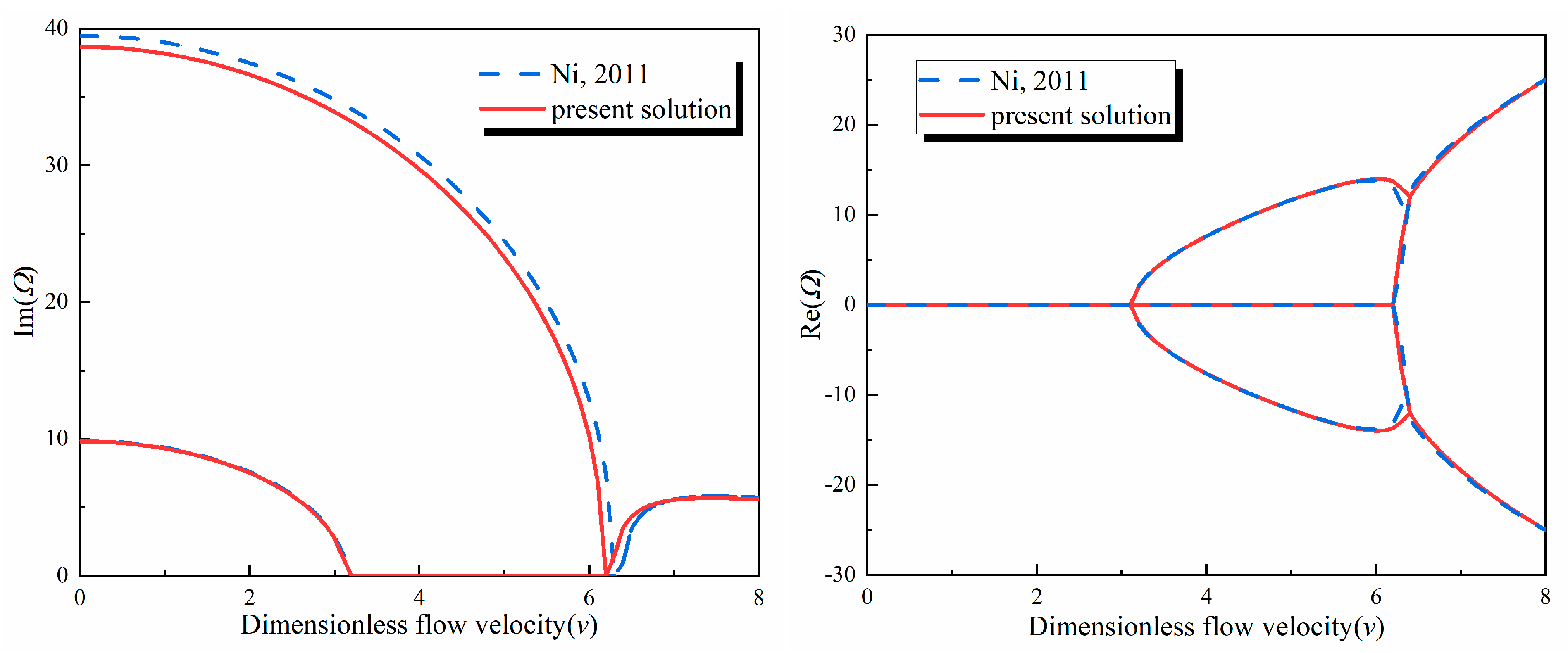
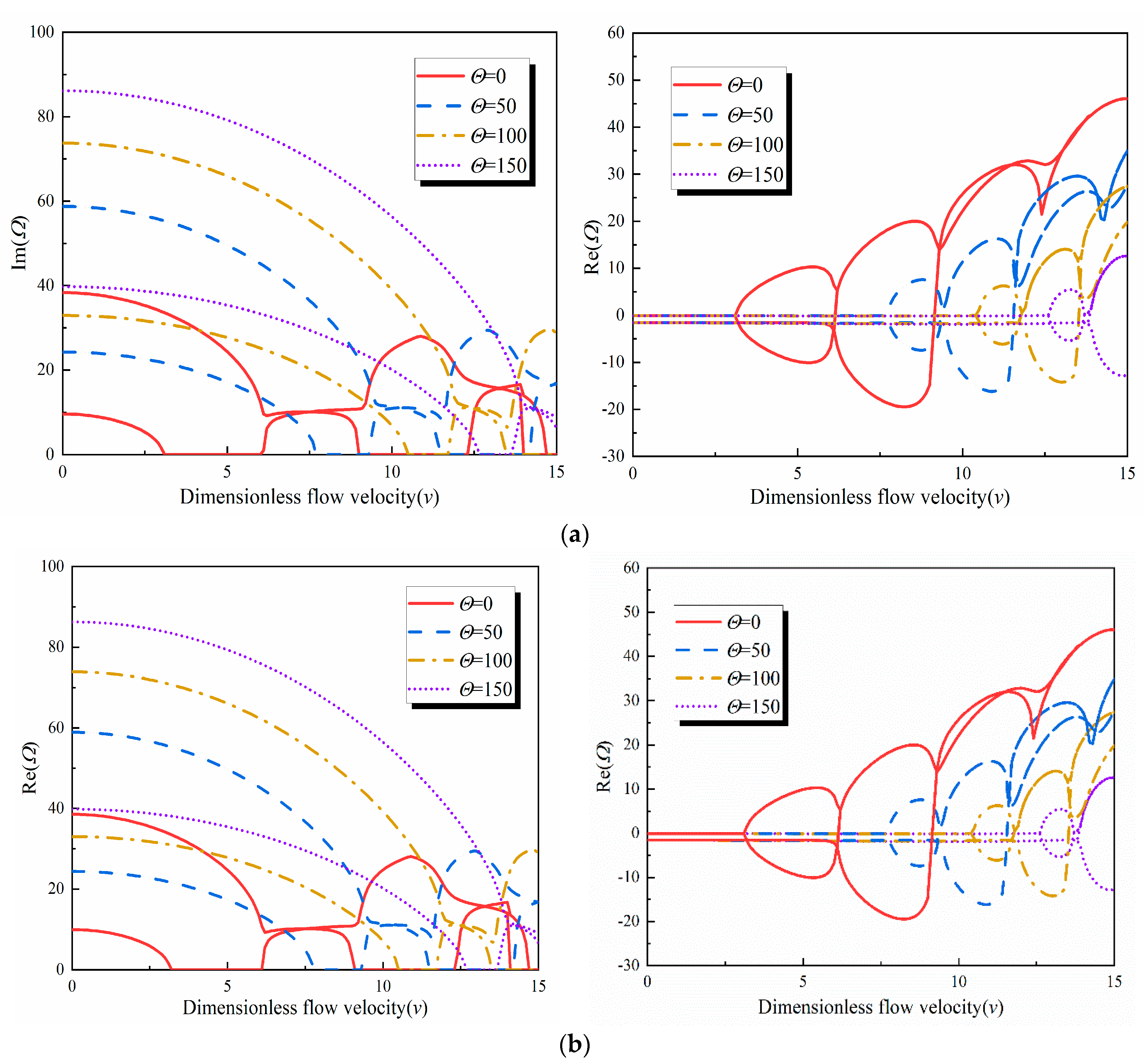
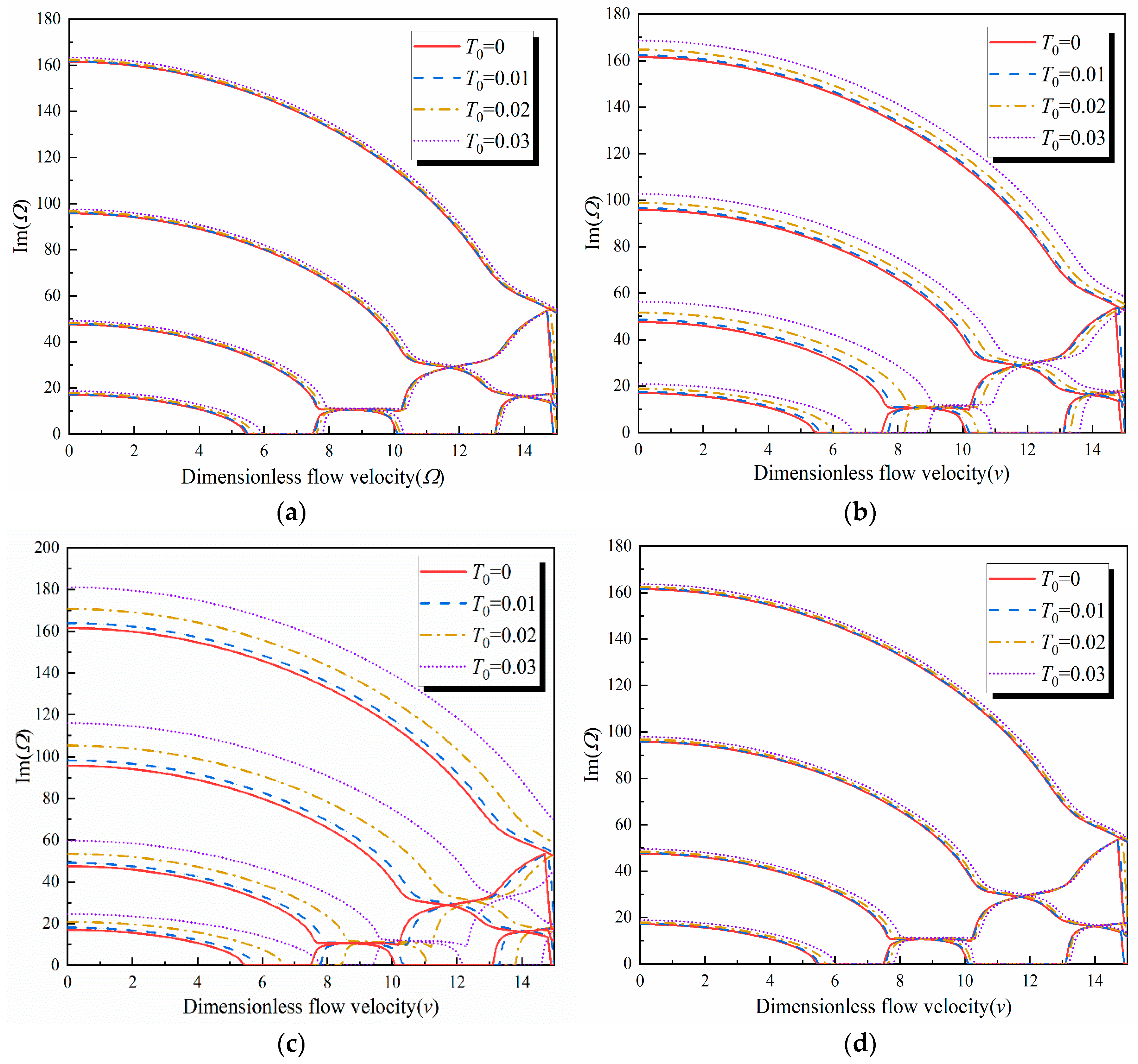
4. Calculation Example

To validate the calculation method used in this solution, we removed the temperature and magnetic field terms from Equation (46), whereas the other items in Equation (46) were set according to the literature parameters. Subsequently, the results obtained using this method were compared with those found in the literature [46]. Figure 2 shows that the calculated results from both methods highly agree, demonstrating the effectiveness of Galerkin’s method for solving the model presented in this paper.

In this section, through numerical calculations, we analyze the effect of dimensionless temperature field parameters, dimensionless magnetic field parameters, initial geometric defect type, power-law exponent, and thermal–magnetic coupling on the dimensionless complex frequency of a simply supported FGV fluid-conveying pipe with initial geometric defects in a thermal–magnetic coupling field. We set Poisson’s ratio as μ = 0.3 and the ratio of the inner radius of the pipe to the outer radius as $R_i/R_o=0.85 .$ Additionally, we consider the ratio of pipe length to pipe diameter $L/d=10$, the relationship between viscosity coefficients, and the elastic modulus of materials inside and outside the pipe. Furthermore, we set ${\eta }_i/E_i={10}^{-7} ; {\eta }_o/E_o={10}^{-7} ,$ and we assume the relationship between the shear moduli and elastic moduli of materials inside and outside the pipe to be $G_i=\frac{E_i}{2\left(1+\mu \right)} , G_o=\frac{E_o}{2\left(1+\mu \right)} .$ The pipe is composed of two materials, transitioning from a pure ceramic surface of SiC on the inner surface to a pure metal surface of Al on the outside. The material characteristics of the pipe are presented in

Table 1. Material characteristics of pipe [47].

Notation	Name (Inner Surface)	Value	Notation	Name (Outer Surface)	Value
${\rho }_i$	Density	$3000{ \mathrm{kg}/\mathrm{m}}^3$	${\rho }_o$	Density	$2{700 \mathrm{kg}/\mathrm{m}}^3$
$E_i$	Young’s modulus	427 GPa	$E_o$	Young’s modulus	69 GPa
${\alpha }_i$	Coefficient of thermal expansion	$4.7\times {10}^{-6}{\mathrm{K}}^{-1}$	${\alpha }_i$	Coefficient of thermal expansion	$23\times {10}^{-6}{\mathrm{K}}^{-1}$

.

Considering the dimensionless magnetic field parameters Θ = 50, the initial geometric defect was of the half-sinusoidal wave type. In the following description, “Im” represents the imaginary parts of the pipe dimensionless complex frequencies, also known as the complex frequencies, and “Re” represents the real parts, also known as the internal damping.

Figure 3 shows the dimensionless complex frequency of a fluid-conveying pipe versus the dimensionless flow velocity under different thermal fields. As the temperature field parameter remains fixed, with a gradual increase in the dimensionless velocity v, the first two-order imaginary parts of the pipe progressively decrease until reaching zero, whereas the real parts remain at zero. Continuously increasing the dimensionless velocity leads to the imaginary parts decreasing to zero and intersecting the x-axis; the dimensionless velocity corresponding to this intersection is referred to as the dimensionless critical velocity. Further increasing the dimensionless flow velocity results in the first-order imaginary part curve remaining at zero, while the real parts gradually increase. This behavior arises from the first-order vibration stiffness of the pipe diminishing to zero, causing the FGV fluid-conveying pipe to enter an unstable state. Subsequently, as the dimensionless flow velocity continues to increase, the first two-order imaginary part curves no longer overlap, indicating the absence of coupling flutter in this FGV fluid-conveying pipe system. Concurrently, the real parts are not symmetrical about the x-axis, suggesting that the system exhibits damped vibrations.

As the dimensionless temperature axial force increases, both the dimensionless complex frequency imaginary parts and the critical velocity of the FGV fluid-conveying pipe decrease. Moreover, at the same velocity, the imaginary parts of the dimensionless complex frequency decrease with increasing dimensionless temperature axial force. The initial geometric defect amplitude shown in Figure 3 reveals that under the same condition, the variation patterns of pipes with initial geometric defects and those without initial geometric defects in the thermal environment are essentially the same and that the increase in the dimensionless temperature axial force leads to a reduction in the first two imaginary parts and the corresponding critical velocity. This finding implies that reducing the temperature variations can effectively improve the stability of the FGV fluid-conveying pipe.

As shown in Figure 4, for a material power-law exponent k = 10 and dimensionless temperature parameter Φ = 0, the first two-order complex frequencies and dimensionless critical velocity of the FGV fluid-conveying pipe increase with increasing dimensionless magnetic force. Under the same dimensionless flow velocity, the larger the dimensionless magnetic field force, the larger the corresponding dimensionless complex frequency imaginary part. Under the same magnetic field environment, the variation law of the dimensionless complex frequency of the pipe with the dimensionless velocity is identical to the variation law of the viscoelastic pipe in the non-magnetic field environment.

Figure 4b shows the amplitude of the initial geometric defect for $T_0=0.01.$ The variation law of the fluid-conveying pipe with initial geometric defect is the same as that of the pipe without initial geometric defect in the magnetic field. As the axial force of the magnetic field increases, the first two-order imaginary part and critical velocity increase. The results show that increasing the magnetic field intensity can effectively improve the stability of the FGV fluid-conveying pipe.

So far, we have studied the influence of a single variable on the complex frequency of the pipe. Here, we study the effects of thermal–magnetic coupling on the vibration complex frequencies of the FGV fluid-conveying pipe with initial geometric defects. To this end, we set the initial geometric defect as a half-sinusoidal wave, with the amplitude of the defect T₀ = 0.03; the dimensionless temperature parameters are Φ = 10 and Φ = 30, and and the dimensionless magnetic field parameters are Θ = 50 and Θ = 100.

As shown in Figure 5, when the critical velocity for Φ = 10 and Θ = 50 is greater than that for Φ = 30 and Θ = 50 but smaller than that corresponding to Φ = 30 and Θ = 100, and when the critical velocity corresponding to Φ = 30 and Θ = 100 is smaller than that corresponding to Φ = 10 and Θ = 100, the magnetic field can enhance the critical flow velocity of the system, whereas the temperature variation can reduce it. Because the temperature variation and the magnetic field have opposite effects on the dynamic characteristics of the system, controlling the temperature variation and increasing the magnetic field intensity can be used as an effective means to improve the vibration stability of FGV fluid-conveying pipes with initial geometric defects under thermal–magnetic coupling. Therefore, the pipe design flow velocity required for practical engineering applications can be attained by increasing the external magnetic field strength and controlling the temperature variation around the pipe.

Figure 6 shows the dimensionless complex frequency for a dimensionless temperature parameter Φ = 30 and dimensionless magnetic field parameter Θ = 50. Four different initial geometric defect types are considered: the quadratic parabolic type: $W_0\left(\overline{x}\right)=4T_0\overline{x}(1-\overline{x}),$ half-sinusoidal wave type: $W_0\left(\overline{x}\right)=T_0\sin (\pi \overline{x})$, one-sinusoidal wave type: $W_0\left(\overline{x}\right)=T_0\sin (2\pi \overline{x})$, and one-and-a-half-sinusoidal wave type: $W_0\left(\overline{x}\right)=T_0\sin (3\pi \overline{x}).$

As evident from Figure 6, when dimensionless magnetic field parameters and dimensionless temperature parameters are fixed, the natural frequencies of each order of the four different types of initial geometric defect pipes all increase with increasing initial geometric defects. The variation of the initial geometric defect amplitude significantly influences the natural frequency of the FGV fluid-conveying pipes with one-sinusoidal wave type and one-and-a-half-sinusoidal wave type geometric defects, as compared to the half-sinusoidal wave type and quadratic parabolic type initial geometric defects. For quadratic parabolic type and half-sinusoidal wave type initial geometric defects, the change laws are essentially identical. With increasing initial geometric defect amplitude, the first four orders of dimensionless natural frequency increase. Further, the change in the initial geometric defect amplitude has an evident effect on the first order of the natural frequency. For the one-sinusoidal wave type initial geometric defect, the first four dimensionless natural frequencies increase with increasing initial geometric defect amplitude, and the change in the initial geometric defect amplitude has the most pronounced effect on the second order of the natural frequency. For the one-and-a-half sinusoidal wave type initial geometric defect, the natural frequencies of each order increase with increasing initial geometric defect amplitude; however, a change in the initial geometric defect amplitude has the most pronounced effect on the third order of the natural frequency.

As shown in Figure 7, under a thermal–magnetic coupling field, the imaginary parts of each order in FGV fluid-conveying pipes with and without initial geometric defects follow a similar change pattern with the power-law exponent. As the power-law exponent increases, the first two imaginary parts of the FGV fluid-conveying pipes increase. The change is more noticeable when k < 10 because the elastic modulus of the model increases rapidly with increasing k, thus resulting in a rapid increase in the stiffness of the system, making it more stable. As the power-law exponent continues to increase, the stiffness of the pipe changes little, and the system gradually stabilizes. Therefore, the power-law exponent determines the effect of the stiffness of the pipe on the stability of the entire fluid-conveying pipe system; reasonable selection of the power-law exponent is critical to pipe design.

5. Conclusions

Through the application of the Hamilton principle, a nonlinear differential equation of motion was derived for an FGV fluid-conveying pipe with an initial geometric curvature under a thermal–magnetic coupling field. The nonlinear terms within the equation were linearized using an analytical method, thus transforming the equation into a dimensionless linear one that was subsequently solved discretely utilizing the Galerkin method. Finally, the factors affecting the stability of the system were analyzed. The following conclusions were drawn:

• The presence of initial geometric defects does not eliminate the influence of temperature and magnetic fields on the stability of the FGV fluid-conveying pipe. Specifically, the stability of the FGV fluid-conveying pipe decreases with increasing temperature but increases with increasing magnetic field intensity. When both the temperature difference and magnetic field intensity increase simultaneously, they counterbalance each other.
• The natural frequencies of each order of pipes with different types of initial geometric defects increase with the amplitude of the initial geometric defect. For pipes with initial geometric defects of the quadratic parabolic and half-sinusoidal wave types, the change in amplitude primarily influences the first-order imaginary part. For initial geometric defects of the single-sinusoidal wave type, the change in amplitude has the most evident effect on the second-order imaginary part. When initial geometric defects take the form of a half-sinusoidal wave, the third-order imaginary part is most influenced by changes in amplitude.
• As the power-law exponent increases, the first two imaginary parts of the system increase, with the most significant variation occurring in the range of 0–10. This phenomenon arises because an increase in the power-law exponent results in a rapid rise in the elastic modulus of the pipe, subsequently leading to a substantial increase in the stiffness of the pipe system and enhanced stability. With further increase in the power-law exponent, the stiffness of the pipe undergoes only slight changes, and the system gradually achieves greater stability. Therefore, the careful selection of the power-law exponent is important for pipe design.

References

1. Païdoussis, M.P.; Issid, N.T. Dynamic stability of pipes conveying fluid. J. Sound Vib. 1974, 33, 267–294. [Google Scholar] [CrossRef]
2. Dai, H.L.; Wang, L.; Qian, Q.; Ni, Q. Vortex-induced vibrations of pipes conveying pulsating fluid. Ocean Eng. 2014, 77, 12–22. [Google Scholar] [CrossRef]
3. Aldraihem, O.J. Analysis of the dynamic stability of collar-stiffened pipes conveying fluid. J. Sound Vib. 2007, 300, 453–465. [Google Scholar] [CrossRef]
4. Tang, Y.; Yang, T. Post-buckling behavior and nonlinear vibration analysis of a fluid-conveying pipe composed of functionally graded material. Compos. Struct. 2018, 185, 393–400. [Google Scholar] [CrossRef]
5. Jin, J.D. Stability and chaotic motions of a restrained pipe conveying fluid. J. Sound Vib. 1997, 208, 427–439. [Google Scholar] [CrossRef]
6. Kheiri, M. Nonlinear dynamics of imperfectly-supported pipes conveying fluid. J. Fluids Struct. 2020, 93, 102850. [Google Scholar] [CrossRef]
7. Li, S.; Karney, B.W.; Liu, G. FSI research in pipeline systems—A review of the literature. J. Fluids Struct. 2015, 57, 277–297. [Google Scholar] [CrossRef]
8. Erdogan, F. Fracture mechanics of functionally graded materials. Compos. Eng. 1995, 5, 753–770. [Google Scholar] [CrossRef]
9. Imek, M. Fundamental frequency analysis of functionally graded beams by using different higher-order beam theories. Nucl. Eng. Des. 2010, 240, 697–705. [Google Scholar] [CrossRef]
10. Fallah, A.; Aghdam, M.M. Nonlinear free vibration and post-buckling analysis of functionally graded beams on nonlinear elastic foundation. Eur. J. Mech. A Solids 2011, 30, 571–583. [Google Scholar] [CrossRef]
11. Shen, H.; Païdoussis, M.P.; Wen, J.; Yu, D.; Wen, X. The beam-mode stability of periodic functionally-graded-material shells conveying fluid. J. Sound Vib. 2014, 333, 2735–2749. [Google Scholar] [CrossRef]
12. Wattanasakulpong, N.; Ungbhakorn, V. Linear and nonlinear vibration analysis of elastically restrained ends FGM beams with porosities. Aerosp. Sci. Technol. 2014, 32, 111–120. [Google Scholar] [CrossRef]
13. Zhu, B.; Xu, Q.; Li, M.; Li, Y. Nonlinear free and forced vibrations of porous functionally graded pipes conveying fluid and resting on nonlinear elastic foundation. Compos. Struct. 2020, 252, 112672. [Google Scholar] [CrossRef]
14. Khodabakhsh, R.; Saidi, A.R.; Bahaadini, R. An analytical solution for nonlinear vibration and post-buckling of functionally graded pipes conveying fluid considering the rotary inertia and shear deformation effects. Appl. Ocean Res. 2020, 101, 102277. [Google Scholar] [CrossRef]
15. Xu, W.; Pan, G.; Moradi, Z.; Shafiei, N. Nonlinear forced vibration analysis of functionally graded non-uniform cylindrical microbeams applying the semi-analytical solution. Compos. Struct. 2021, 275, 114395. [Google Scholar] [CrossRef]
16. Rezaiee-Pajand, M.; Masoodi, A.R. Analyzing FG shells with large deformations and finite rotations. World J. Eng. 2019, 16, 636–647. [Google Scholar] [CrossRef]
17. Rezaiee-Pajand, M.; Masoodi, A.R. Stability analysis of frame having FG tapered beam-column. Int. J. Steel Struct. 2019, 19, 446–468. [Google Scholar] [CrossRef]
18. Masoodi, A.R.; Ghandehari, M.A.; Tornabene, F.; Dimitri, R. Natural frequency response of FG-CNT coupled curved beams in thermal conditions. Appl. Sci. 2024, 14, 687. [Google Scholar] [CrossRef]
19. Rajidi, S.R.; Gupta, A.; Panda, S. Vibration characteristics of viscoelastic sandwich tube conveying fluid. Mater. Today Proc. 2020, 28, 2440–2446. [Google Scholar] [CrossRef]
20. Amirinezhad, H.; Tarkashvand, A.; Talebitooti, R. Acoustic wave transmission through a polymeric foam plate using the mathematical model of functionally graded viscoelastic (FGV) material. Thin-Walled Struct. 2020, 148, 106466. [Google Scholar] [CrossRef]
21. Deng, J.Q.; Liu, Y.S.; Zhang, Z.J.; Liu, W. Stability analysis of multi-span viscoelastic functionally graded material pipes conveying fluid using a hybrid method. Eur. J. Mech. A Solids 2017, 65, 257–270. [Google Scholar] [CrossRef]
22. Deng, J.Q.; Liu, Y.; Zhang, Z.; Liu, W. Size-dependent vibration and stability of multi-span viscoelastic functionally graded material nanopipes conveying fluid using a hybrid method. Compos. Struct. 2017, 179, 590–600. [Google Scholar] [CrossRef]
23. Hosseini-Hashemi, S.; Abaei, A.R.; Ilkhani, M.R. Free vibrations of functionally graded viscoelastic cylindrical panel under various boundary conditions. Compos. Struct. 2015, 126, 1–15. [Google Scholar] [CrossRef]
24. Pinnola, F.P.; Barretta, R.; de Sciarra, F.M.; Pirrotta, A. Analytical solutions of viscoelastic nonlocal Timoshenko beams. Mathematics 2022, 10, 477. [Google Scholar] [CrossRef]
25. Fu, G.M.; Tuo, Y.H.; Zhang, H.; Su, J.; Sun, B.; Wang, K.; Lou, M. Effects of material characteristics on nonlinear dynamics of viscoelastic axially functionally graded material pipe conveying pulsating fluid. J. Mar. Sci. Appl. 2023, 22, 247–259. [Google Scholar] [CrossRef]
26. Akintoye, O.O.; Oyediran, A.A. The effect of various boundary conditions on the nonlinear dynamics of slightly curved pipes under thermal loading. Appl. Math. Model. 2020, 87, 332–350. [Google Scholar] [CrossRef]
27. Fu, Y.M.; Zhong, J.; Shao, X.F.; Chen, Y. Thermal postbuckling analysis of functionally graded tubes based on a refined beam model. Int. J. Mech. Sci. 2015, 96–97, 58–64. [Google Scholar] [CrossRef]
28. Ghorbanpour Arani, A.; Haghparast, E.; Ghorbanpour Arani, A.H. Size-dependent vibration of double-bonded carbon nanotube-reinforced composite microtubes zconveying fluid under longitudinal magnetic field. Polym. Compos. 2016, 37, 1375–1383. [Google Scholar] [CrossRef]
29. Ma, T.; Mu, A. Study on the stability of functionally graded simply supported fluid-conveying microtube under multi-physical fields. Micromachines 2022, 13, 895. [Google Scholar] [CrossRef]
30. Lu, Q.S.; To, C.W.S.; Huang, K.L. Dynamic stability and bifurcation of an alternating load and magnetic field excited magnetoelastic beam. J. Sound Vib. 1995, 181, 873–891. [Google Scholar] [CrossRef]
31. Zhou, Y.H.; Gao, Y.W.; Zheng, X.; Jiang, Q. Buckling and post-buckling of a ferromagnetic beam-plate induced by magnetoelastic interactions. Int. J. Non-Linear Mech. 2000, 35, 1059–1065. [Google Scholar] [CrossRef]
32. Wu, G.Y. The analysis of dynamic instability and vibration motions of a pinned beam with transverse magnetic fields and thermal loads. J. Sound Vib. 2005, 284, 343–360. [Google Scholar] [CrossRef]
33. Hosseini, M.; Sadeghi-Goughari, M. Vibration and instability analysis of nanotubes conveying fluid subjected to a longitudinal magnetic field. Appl. Math. Model. 2016, 40, 2560–2576. [Google Scholar] [CrossRef]
34. Pisarski, D.; Konowrocki, R.; Szmidt, T. Dynamics and optimal control of an electromagnetically actuated cantilever pipe conveying fluid. J. Sound Vib. 2018, 432, 420–436. [Google Scholar] [CrossRef]
35. Zhong, J.; Fu, Y.M.; Wan, D.T.; Li, Y. Nonlinear bending and vibration of functionally graded tubes resting on elastic foundations in thermal environment based on a refined beam model. Appl. Math. Model. 2016, 40, 7601–7614. [Google Scholar] [CrossRef]
36. Chen, X.; Zhao, J.L.; She, G.L.; Jing, Y.; Pu, H. Nonlinear free vibration analysis of functionally graded carbon nanotube reinforced fluid-conveying pipe in thermal environment. Steel Compos. Struct. 2022, 45, 641–652. [Google Scholar] [CrossRef]
37. Li, Z.M.; Qiao, P. Buckling and postbuckling behavior of shear deformable anisotropic laminated beams with initial geometric imperfections subjected to axial compression. Eng. Struct. 2015, 85, 277–292. [Google Scholar] [CrossRef]
38. Ding, H.X.; She, G.L.; Zhang, Y.W. Nonlinear buckling and resonances of functionally graded fluid-conveying pipes with initial geometric imperfection. Eur. Phys. J. Plus 2022, 137, 1329. [Google Scholar] [CrossRef]
39. Liu, H.; Lv, Z.; Tang, H.J. Nonlinear vibration and instability of functionally graded nanopipes with initial imperfection conveying fluid. Appl. Math. Model. 2019, 76, 133–150. [Google Scholar] [CrossRef]
40. Zhu, B.; Chen, X.C.; Guo, Y.; Li, Y.-H. Static and dynamic characteristics of the post-buckling of fluid-conveying porous functionally graded pipes with geometric imperfections. Int. J. Mech. Sci. 2021, 189, 105947. [Google Scholar] [CrossRef]
41. Farshidianfar, A.; Soltani, P. Nonlinear flow-induced vibration of a SWCNT with a geometrical imperfection. Comput. Mater. Sci. 2012, 53, 105–116. [Google Scholar] [CrossRef]
42. Tong, G.J.; Liu, Y.S.; Cheng, Q.; Dai, J. Stability analysis of cantilever functionally graded material nanotube under thermo-magnetic coupling effect. Eur. J. Mech. A Solids 2020, 80, 103929. [Google Scholar] [CrossRef]
43. Hamed, H.; Tawfik, M.; Negm, H.M. Thermal buckling and nonlinear flutter behavior of shape memory alloy hybrid composite plates. J. Vib. Control 2011, 17, 489–503. [Google Scholar] [CrossRef]
44. Matouk, H.; Bousahla, A.A.; Houari, H.; Bourada, F.; El Abbas, A.B.; Tounsi, A.; Mahmound, S.R.; Benrahou, K.H. Investigation on hygro-thermal vibration of P-FG and symmetric S-FG nanobeam using integral Timoshenko beam theory. Adv. Nano Res. 2020, 8, 293–305. [Google Scholar] [CrossRef]
45. Zhen, Y.X.; Gong, Y.F.; Tang, Y. Nonlinear vibration analysis of a supercritical fluid-conveying pipe made of functionally graded material with initial curvature. Compos. Struct. 2021, 268, 113980. [Google Scholar] [CrossRef]
46. Ni, Q.; Zhang, Z.L.; Wang, L. Application of the differential transformation method to vibration analysis of pipes conveying fluid. Appl. Math. Comput. 2011, 217, 7028–7038. [Google Scholar] [CrossRef]
47. Loghman, E.; Kamali, A.; Bakhtiari-Nejad, F.; Abbaszadeh, M. Nonlinear free and forced vibrations of fractionally modeled viscoelastic FGM micro-beam. Appl. Math. Model. 2021, 92, 297–314. [Google Scholar] [CrossRef]
Figure 1. Dynamic model of FGV fluid-conveying pipe with initial geometric defects under thermal–magnetic coupling field.
Mathematics 12 00840 g001
Figure 2. Comparison of the present results with Ni’s results [46].
Mathematics 12 00840 g002
Figure 3. Complex frequencies vs. dimensionless flow velocity for different temperature parameters (k = 10, Θ = 50). (a) T0 = 0. (b) T0 = 0.01.
Mathematics 12 00840 g003
Figure 4. First two-order complex frequency of the model vs. dimensionless flow velocity at different magnetic field parameters (k = 10, Φ = 0). (a) T0 = 0. (b) T0 = 0.
Mathematics 12 00840 g004
Figure 5. Dimensionless complex frequency of the model with dimensionless velocity for different physical fields (k = 10, T 0 = 0.03 ).
Mathematics 12 00840 g005
Figure 6. First four-order imaginary parts of the FGV fluid-conveying pipe with different dimensionless flow velocities (k = 10, Φ = 30, Θ = 50). (a) Half-sinusoidal wave type, (b) One-sinusoidal wave type, (c) One-and-a-half-sinusoidal wave type, (d) Quadratic parabolic type.
Mathematics 12 00840 g006
Figure 7. Imaginary parts of the FGV fluid-conveying pipe vs. power-law exponent for Φ = 30 and Θ = 50. (a) T 0 = 0 . (b) T 0 = 0.01 .
Mathematics 12 00840 g007