Algorithms for the Reconstruction of Genomic Structures with Proofs of Their Low Polynomial Complexity and High Exactness

Abstract

The mathematical side of applied problems in multiple subject areas (biology, pattern recognition, etc.) is reduced to the problem of discrete optimization in the following mathematical method. We were provided a network and graphs in its leaves, for which we needed to find a rearrangement of graphs by non-leaf nodes, in which the given functional reached its minimum. Such a problem, even in the simplest case, is NP-hard, which means unavoidable restrictions on the network, on graphs, or on the functional. In this publication, this problem is addressed in the case of all graphs being so-called “structures”, meaning directed-loaded graphs consisting of paths and cycles, and the functional as the sum (over all edges in the network) of distances between structures at the endpoints of every edge. The distance itself is equal to the minimal length of sequence from the fixed list of operations, the composition of which transforms the structure at one endpoint of the edge into the structure at its other endpoint. The list of operations (and their costs) on such a graph is fixed. Under these conditions, the given discrete optimization problem is called the reconstruction problem. This paper presents novel algorithms for solving the reconstruction problem, along with full proofs of their low error and low polynomial complexity. For example, for the network, the problem is solved with a zero error algorithm that has a linear polynomial computational complexity; and for the tree the problem is solved using an algorithm with a multiplicative error of at most two, which has a second order polynomial computational complexity.

1. Introduction

Biological problems of reconstructing genes, genomes, genome syntenies, cell types and their annotations take up a central place in modern genomics. These biological problems are addressed in hundreds of publications, of which we would like to highlight reviews [1,2]. Well-known algorithms for such reconstruction are of a heuristic nature; most notably, they are not accompanied with evidential estimations of the algorithm’s accuracy and error in standard form; such mathematical questions are not even usually addressed in these publications. Among the algorithms of genome reconstruction, we highlight [3] a convenient way of visualizing reconstructed genomes when working with databases [4]. In regard to the biological problem of reconstructing genome syntenies, we highlight the review [5]; and among the algorithms of its solution [6,7]. On reconstructing cell types, we highlight the work presented in [8,9]; in the latter, a network class is introduced with node marks that are convenient for describing cell types and their evolution.

From these biological reconstruction problems, and especially from the problem of reconstructing genome syntenies, a mathematical reconstruction problem arose along the network of graphs of a special type, called genomic structures. Recall that a genomic structure (hereafter referred to simply as a structure) is any directed graph whose components are paths and cycles (including loops, but not isolated nodes), and whose edges are assigned with names, for example, natural numbers. In other words, the degree of each node of the graph is either 1 or 2. Such a representation of a biological genome as a set of linear and circular chromosomes has been studied in biology for about thirty years. The formulation of the corresponding mathematical problem is based on a fixed set of SCJ or DCJ operations, each of which is assigned a cost, a strictly positive rational number.

Recall that SCJ (Single-Cut-or-Join) operations are the following: a merge (join) of two free extremities of edges at one node of the graph and a cut (the inverse of a join, cutting a node of degree 2); in the case of unequal sets of edge names of structures, two more operations are added here: insertion of an isolated edge and its deletion; see [10]. The set of edge names is called the content of a structure.

Recall that DCJ (Double-Cut-and-Join) operations are as follows:

(1)

Double inter-merging. Cut two nodes in the structure and merge (join) the four resulting free extremities.

(2)

Sesquialteral inter-merging. Cut a node and merge (join) one resulting in free extremity with any free extremity in the structure.

(3–4)

Single inter-mergings: cut and join (mutually inverse operations): undo a merge of extremities at one node, or join two free extremities together; see [11].

As above, if structures a and b have unequal sets of edge names (say: unequal contents), two more operations are added here: insertion of a connected fragment of edges belonging to b but not to a into a component of a (or as its separate component), and deletion of such a fragment of edges belonging to a but not to b from a.

Thus, equal gene content of two genomic structures means that they have the same number of genes and a one-to-one orthology correspondence is defined between them. In other words, the names of edges in the structures are unique, and orthologous genes have identical names, i.e., names are not repeated in the structure, and the two sets of structure names coincide. In what follows, unless otherwise specified, we assume that names in a structure are unique. Recall that each operation is assigned with its cost, a strictly positive rational number.

In that way, we come to the definitions. The transformation problem is as follows: for given structures a and b, find a minimal (in the total cost of operations) chain of DCJ operations transforming a into b. For SCJ operations this problem is trivial, but for DCJ operations several dozens of works have been published; we mention below several main contributions. The reconstruction problem for structures defined at leaves of a given network consists of arranging structures at non-leaf nodes of the tree so as to minimize the sum, over all its edges, of the DCJ (or SCJ) distance between the structures assigned to the endpoints of an edge. Here, the DCJ distance is assumed to be the total cost of the minimal (in the total cost of operations) DCJ transformation of the structure closer to the root to the structure closer to the leaves of the tree. The SCJ distance is defined similarly. Actually, the transformation problem is a particular case of the reconstruction problem when a network consists of a single edge. Let us highlight the work presented in [12], which introduces and studies the intermediary structure distance between SCJ and DCJ.

Despite a number of mathematical results, both mathematical problems remain completely nontrivial and far from being finally solved (especially the second one), regardless of their specific applications. In the bioinformatics context, an edge of a structure with its name is called a gene, and a component of the structure is called a chromosome. The structure itself is sometimes referred to as the genome. Describing a biological genome as a structure, of course, neglects most of its actual features but, nevertheless, it is useful to study the properties of the biological genome. One of the reasons for this usefulness is that structures allow efficient algorithms that are guaranteed to cope with hundreds of genes simultaneously. In essence, a structure describes the gene synteny, and algorithms allow us, among other things, to reconstruct the gene synteny and to identify ancient and stable syntenies and their evolutions.

In this publication, authors study the second problem—the reconstruction problem—specifically as a mathematical one, not touching on its multiple applications. The mathematical hardness of this problem is described through the fact that for the DCJ distance, the reconstruction problem is NP-hard even for a tree consisting of a root and three leaves with equal gene content [13]. For the SCJ distance, the reconstruction problem seems simpler, although the authors suppose that it is also NP-hard for arbitrary operation costs and even for equal gene content.

In any case, its mathematical solution with a low-polynomial algorithm looks like an extremely interesting and tough challenge in the field of discrete optimization.

To conclude the Introduction, we mention a few papers that have affected our interest in this biological subject, first on transformation and then on reconstruction problems.

Among the pioneers who set and studied these and related problems, we should point out the works of D. Sankoff, P.A. Pevzner, and their students, referring to surveys [14,15,16].

In the work presented in [17], genomic rearrangements in ancestors of twenty modern mitochondrial genomes were studied. In the work presented in [18], genomes consisting of a single chromosome and a reversal operation were considered, and the shortest sequence of reversals reducing an initial sequence of integers to a strictly increasing sequence of positive numbers was constructed. The resulting algorithm has degree-four polynomial runtime. In the work presented in [19] the problem of determining the distance between two genomes was considered in which the chromosome is a sequence of nonzero integers. The operations of fusion, fission, reversal, and translocation were allowed; the corresponding algorithm with degree-four polynomial complexity was obtained. In the work presented in [20], an important original construction of a breakpoint graph was proposed, in which we generalized to the case of unequal gene content [21]. In the work presented in [19], a reduction of the genome transformation problem to the problem of reducing a breakpoint graph to a final form was proposed, which we later generalized to the case of unequal gene content [21].

In the work presented in [11], a linear-time algorithm was proposed for solving the transformation problem with equal gene content of structures and equal operation costs (i.e., in their absence). In the work presented in [22,23], linear-time algorithms are described for solving this problem under unequal gene content and equal operation costs. In the work presented in [24,25,26] linear-time algorithms are described for solving this problem with unequal gene content and partially unequal operation costs: the costs of the first four DCJ operations are equal; the costs of insertion and deletion operations are also equal but possibly different from the cost of the first four operations. In the work presented in [21,27] a linear-time algorithm is described for solving this problem with unequal gene content and unequal operation costs: the costs of the first four DCJ operations are equal (denote them by c), the costs w_i and w_d of insertion and deletion operations may be unequal to each other and unequal to c. If c ≤ min(w_i,w_d) < max(w_i,w_d), then our algorithm may admit an additive error k ≤ 2c. If min(w_i,w_d) < c < max(w_i,w_d), then we have k ≤ max(w_i,w_d) − c (if w_d + w_i ≤ 2c), k ≤ 4·max(w_i,w_d) + 2·min(w_i,w_d) − 6c (if w_d + w_i > 2c and max(w_i,w_d) ≤ 2c) and k ≤ 6·max(w_i,w_d) + 2·min(w_i,w_d) − 9c (if max(w_i,w_d) > 2c).

A separate difficult question is whether topological properties of structures a and b can be preserved in intermediate structures of the shortest (or close to it) transformation of a into b? In the case of equal gene content of a and b, the following partial results have been obtained [28] (Section 6):

(1)

Let structures a and b have equal content, and let each of them consist of a single cycle. There exists a quadratic-time algorithm which outputs a shortest transformation of a into b such that every intermediate structure in it consists of at most two cycles; if the second cycle appears at some step, then at the next step there remains a single cycle again.

(2)

Let structures a and b have equal content, and let each of them consist of a single path. There exists a quadratic-time algorithm which outputs the shortest transformation of a into b such that any intermediate structure in it consists of at most one path and one cycle; if a cycle appears, then at the next step there remains a single path again.

(3)

Let structures a and b have equal content, and let each of them consist of paths. There exists a quadratic-time algorithm which outputs the shortest transformation of a into b such that any intermediate structure in it consists of at most one cycle; if a cycle appears, then at the next step there remain only paths again.

Let us now touch upon the case where different edges of a structure can have equal names, i.e., there are paralogs in the structure. Then, the transformation problem is NP-hard for SCJ operations [29,30] and for DCJ operations [31,32]. A reduction of this problem to an integer linear programming problem is known, e.g., in the work presented in [33]. Its direct solution (i.e., not by reducing this problem to another one) by an algorithm of polynomial complexity assumes constraints imposed on the initial structures and/or on the list of operations over structure. For example, in the work presented in [34], paralogs are not allowed in structure a but are allowed in structure b, sets of names in a and b are equal (so-called “quasi-equal content”), while only cut and join operations are allowed and, additionally, an additional operation of edge duplication: inserting a new edge next to a given edge, with the same name and orientation (“linear duplication”), or adding an edge with the same name in the form of a loop as a separate component of the structure (“cyclic duplication”). A reminder here: the edges of the structure that have identical names are called paralogs; the results of this publication relate to structures without paralogs, even though those are sometimes mentioned in the description of other authors’ publications. Item [35] describes approximated algorithms for calculating various distances between paralog structures, considering not only their genetic composition, but also the distance between neighboring genes. Algorithm error scores proved to be proportional to the maximum number of gene paralogs in a structure.

We considered another constraint on a and b with quasi-equal content: as above, a has no paralogs, and b has at most two paralogs of each edge; however, all DCJ operations over the structure are allowed together with the duplication operation, and costs of the operations are arbitrary [28] (Section 1). This problem is already NP-hard [28]. For this problem, the authors have obtained an algorithm that constructs a transformation of a into b with multiplicative error of at most 13/9 + ε, where ε is any strictly positive number; its runtime is of the order of $n^{O({\epsilon }^{-2.6})}$, where n is the size of the initial pair of graphs a and b [28].

Item [36] describes the algorithm for solving the reconstruction problem for structures with an equal genetic composition on a tree that consists of a root and three leaves; at that, DCJ operations are used, and a certain evaluation of the algorithm’s accuracy is received. In the work presented in [37] (Section 3.6), a reduction of the reconstruction problem to a sequence of SAT problems is described for a star, i.e., a tree consisting of a root and arbitrarily many leaves. There, we assumed structures consisting of circular chromosomes, equal gene content, and, of course, using the double inter-merging operation only. However, for special cases, efficient algorithms are known. For example, in the work presented in [10], an exact quadratic-time algorithm for structure reconstruction is described for equal SCJ operation costs and equal content of structures. In the work presented in [13], an algorithm is proposed for solving this problem for a star under equal SCJ operation costs and equal content of structures. In [34] this algorithm, also with equal costs, was generalized to the case of quasi-equal content (no paralogs at the root) and the operations of cut, join, and duplication. The runtimes of these algorithms are near quadratic. In the work presented in [28] (Section 7), the authors described a (quadratic-time) algorithm for solving the reconstruction problem for a star with equal content of structures and arbitrary costs, or with unequal content but with no paralogs and no loops in the structures. This algorithm admits the requirement that all intermediate structures are cyclic if all given and sought-for structures consist of cycles (cyclic structures). There, the authors have also generalized this algorithm to the case of paralogs in leaf structures, obtaining the following result. Let us provide a star and structures at its leaves with quasi-equal content (i.e., paralogs are allowed). A structure with the same content and without paralogs is searched for at the root, and operations over the structures are cut, join, and duplication (linear and cyclic). Then, by a quadratic-time algorithm, the reconstruction problem can be reduced to the problem of constructing a maximum weighted matching in a complete graph consisting of the extremities of all edges in one of the initial structures. In the work presented in [37] (Section 3), we considered the reconstruction problem on a tree with two non-leaf nodes, where the root is adjacent to arbitrarily many leaves, while a non-root non-leaf node is adjacent to exactly two leaves. There, we have described an algorithm which, for arbitrary SCJ operation costs, solves the reconstruction problem in time of the order of n²l²log(nl), where n is the number of names in the structures assigned to the leaves and l is the number of leaves.

In this paper, we have described novel algorithms for solving the mathematical reconstruction problem for structures on the given network (Section 2 and Section 3), on a general tree (Section 4) and on a specific-type tree (Section 5). All algorithms are accompanied with proofs of their accuracy or evaluations of the maximum possible error. This publication continues the series of the mathematical papers [21,28,37].

2. Reconstruction of Binary States along a Network

2.1. Problem Setting

A phylogenetic network (usually called a network) is a directed acyclic graph in which the nodes are divided into four groups: of in-degree 0 and out-degree ≥ 2 (root), of in-degree 1 and out-degree ≥ 2 (tree-like nodes), of in-degree ≥ 2 and out-degree 1 (hybrid nodes), and of in-degree 1 and out-degree 0 (leaves). If in the definition instead of the condition ≥ 2 we leave the condition = 2, the network is said to be binary. An example of a network is given, for example, in the work presented in [37] (Figure 6); however, in what follows, the network is not assumed to be binary and does not have a root edge. An arrangement of labels along the network is an unambiguous assignment of labels to each node of the network; some of the labels are given, and others are to be found.

Problem: A network is given, and one of the labels 0 or 1 is assigned to each of its leaves. Also, positive rational numbers c₀₁ and c₁₀ are given which are costs of transitions along any edge: if the extremities of an edge are labeled identically, the cost is 0; if the beginning of an edge is labeled with zero and the end with one, it is equal to c₀₁; otherwise, it is equal to c₁₀. The problem is to label all non-leaf nodes with labels 0 or 1 so as to minimize the sum of costs of transitions along all edges. An arrangement, R, of labels is any assignment of labels 0 and 1 to non-leaf nodes of the network; let x(R) be the label at a network node x in an arrangement R. This sum is $H(R)={\displaystyle \sum _{(x,y)}{c}_{xy}|x(R)-y(R)|}$ where the c_xy are as follows: 0 if x(R) = y(R), c₀₁ if x(R) < y(R), and c₁₀ if x(R) > y(R). The sum H(R) will be called the cost of the arrangement R, and an arrangement with the smallest cost will be said to be minimal.

The paper [38] describes an algorithm for solving this problem provided that the costs are equal: c₀₁ = c₁₀ (or, equivalently, in the absence of costs), which is based on its reduction to the maximum flow problem in a network with a source and drain. It is not clear how to generalize that algorithm to the case of unequal costs. We describe an algorithm with a near-linear complexity, which is exact for any costs; it consists of reducing the problem under consideration to a linear programming (LP) problem.

2.2. Description of the Algorithm

To each vertex and each edge in a given network, we assign a variable that takes values in the segment [0, 1]; we call the list of these variables a point in the corresponding multidimensional real space; thus, coordinates of each point are assigned to nodes and edges of the network and are called node and edge variables, respectively. At a leaf, we set the node variables to be equal to the original leaf labels 0 or 1. For each directed edge z = (x,y) starting at x and ending at y, we impose the following constraints: x + y + z ≤ 2, x + z ≥ y, y + z ≥ x, and x + y ≥ z, which define a constraint polytope P. Define the objective function

$$F=\frac{1}{2}{\displaystyle \sum _{z=(x,y)}(c_{10}(z+x-y)+c_{01}(z+y-x))\to \min }$$

(1)

where the sum is taken over all edges of the network. Theorem 1 shows that the minimum point in this LP problem, which is at the same time a vertex of the polytope P, is Boolean, i.e., consists of the numbers 0 and 1. Values of the node variables x and y at this point define the desired minimum labeling of the original network. The size of this LP problem is of the same order as the size of the input data.

In what follows, the abbreviation LP refers to an LP problem as well.

The minimum point in the LP, which is also a vertex of the polytope, can be obtained, for example, by the simplex method. The simplex method is known to work fast, but on some special examples its operation is exponentially long. The interior point algorithm developed in the work presented in [39] (see also [40,41] (Chapter 15)) also runs fast, but still a proved an upper bound on its runtime, expressed by a polynomial of degree 3.5 in the number of variables in the initial LP. In this LP, for a starting point X ∈ P, for example, we can put all node and edge variables (on non-leaf edges) to x = y = z = 0 and (on leaf edges) z = |x − y|. The interior point algorithm terminates at a minimum point Y ∈ P, which is not necessarily a vertex of the polytope. Let F(Y) = c; we define a new polytope P₁ by adding the equation F = c to the constraints of the original polytope P. If F is not a constant, then P₁ is of strictly lower dimension than P. As a new objective function F₁, we choose a linear function that is not a constant on P₁. The same algorithm minimizes F₁ on P₁ by taking Y as a starting point, for example. We repeat these iterations until the next polytope P_i consists of a single vertex, a minimum point of the original function F and at the same time a vertex of the original polytope P. Since the number of iterations is not greater than the number of variables in the objective function F, the overall runtime of the algorithm is estimated by a polynomial of degree 4.5 in the size of the original network. Our computations on a large random sample of initial networks statistically significantly confirm that the heuristic runtime of both of the above-mentioned algorithms is close in order to n·log n, where n is the size of the input data (results of this statistical experiment are not presented here).

Now, let us provide a brief description of the algorithm presented above:

• Input: a network, where the leaves are marked as 0 or 1.
  • For each directed edge z = (x,y) impose the following constraints: x + y + z ≤ 2,
  • x + z ≥ y, y + z ≥ x, x + y ≥ z, x,y,z ≥ 0, x,y,z ≤ 1.
  • Solve the LP minimization problem of the F function, set by expression (1), with these constraints. Obtain a solution at the vertex of the polytope, where all variables equal 0 or 1.
• Output: the given network’s marking with the received values of node variables.

2.3. Exactness of the Algorithm

Theorem 1.

A minimum point of the stated LP problem, which is at the same time as a vertex of the constraint polytope P, defines a minimum arrangement in the original network. The runtime of the algorithm is estimated from above by a polynomial of degree 4.5 in the size of the original network.

Proof. 

At a minimum point of this LP, with coordinates over all nodes x, y, … and over all edges z, …, for each edge z = (x,y), we have z = |x − y|. Indeed, if x ≥ y and z > x − y, then the value of the function can be reduced without leaving the polytope P; the same for the case y ≥ x. Therefore, z = |x − y|.

Assume that at a vertex A of the polytope P the equality z = |x − y| is satisfied for each edge coordinate z = (x,y). Let us verify that any of its node coordinates (and hence its edge coordinates) is Boolean, i.e., A is a Boolean point.

Assuming that some node coordinate at such a point A is equal to d, where 0 < d < 1, we will arrive at a contradiction. Indeed, denote by X the set of network nodes whose node coordinate at A is d. Choose such an ɛ that the segment [d − ɛ, d + ɛ] does not contain the values of the node coordinates at the point A of the network nodes that do not belong to X and does not contain 0 and 1. We reduce by ɛ the value of d in all node coordinates at A of the nodes from X, increase by ɛ the edge coordinates of A on the edges connecting any node in X with any node whose value of its node coordinate at A is strictly greater than d, but reduce by ɛ the values on the edges connecting any node in X with any node whose value of its node coordinate at A is strictly less than d; the other coordinates at A are not changed. The point B obtained in this way belongs to the polytope P, since z₁ = |x₁ − y₁| still holds for its coordinates. Recall the following: if for some point we have z = |x − y| for every edge coordinate z = (x,y) and also x,y ∈ [0, 1], then this point lies in P. Similarly, if we replace all decreases and increases by ɛ with opposite ones, we obtain another point C also belonging to the polytope P (for example, we increase by ɛ the coordinates at C corresponding to the nodes in X). Then, the original point A lies strictly between the points B and C, a contradiction.

Thus, at a vertex A of the polytope P which is a minimum point, values of the node variables define the arrangement R in which F(A) = H(R). If there exists an arrangement R₁ with a cost strictly smaller than H(R), it defines a point D ∈ P if we additionally put z₁ = |x₁ − y₁| for each edge coordinate z₁ = (x₁,y₁). For this point D, we have F(D) = H(R₁) < F(C) = H(R); a contradiction.

The estimate for the runtime of the algorithm immediately follows from the estimate for the runtime of the interior point algorithm; see above. □

Remark 1.

Labels can be defined not only at leaves, but also at some non-leaf nodes of the network. The algorithm for constructing the corresponding conditionally minimal arrangement remains the same: in the function F and in the constraints, the given values should be plugged instead of the corresponding variables. The justification of the algorithm remains the same.

Remark 2.

The claim of Theorem 1 remains true if, instead of a network, we consider an arbitrary directed graph with some selected nodes at which values of an attribute are defined (these vertices play the role of leaves); in this case, each edge is assigned with the costs of two events (change of the attribute in one and in the opposite direction); these costs can also be edge-dependent.

2.4. Example of the Algorithm Operation

Consider a network with input data at the leaves shown in Figure 1a. First, let the transition costs be c₀₁ = c₁₀ = 1. By labeling the nodes and edges of the network with variables as in Figure 1a, we obtain the following LP problem:

min F = 0.5[(x + r − u) + (x + u − r) + (y + r − v) + (y + v − r) + (z + u − w) + (z + w − u) + (t + v − w) + (t + w − v) + (a + u) + (a − u) + (b + w − 1) + (b + 1 − w) + (c + v) + (c − v)] = 0.5[2x + 2y + 2z + 2t + 2a + 2b + 2c] = x + y + z + t + a + b + c under the constraints: r + x + u ≤ 2, r + y + v ≤ 2, u + z + w ≤ 2, v + t + w ≤ 2, u + a ≤ 2, w + b ≤ 1, v + c ≤ 2, r + x ≥ u, r + u ≥ x, x + u ≥ r, r + y ≥ v, r + v ≥ y, y + v ≥ r, u + z ≥ w, u + w ≥ z, z + w ≥ u, v + t ≥ w, v + w ≥ t, t + w ≥ v, u = a, w + b ≥ 1, v = c, and all the variables belong to the segment [0, 1].

The solution of this LP consists of zeros, except for b = 1; it defines a minimal arrangement of labels with cost 1, Figure 1b.

Now let the transition costs be c₀₁ = 3 and c₁₀ = 1. The LP problem differs from the preceding one only in the objective function:

min F = 0.5[(x + r − u) + 3(x + u − r) + (y + r − v) + 3(y + v − r) + (z + u − w) + 3(z + w − u) + (t + v − w) + 3(t + w − v) + (a + u) + 3(a − u) + (b + w − 1) + 3(b + 1 − w) + (c + v) + 3(c − v)] = 2x + 2y + 2z + 2t + 2a + 2b + 2c − 2r − u − v + w + 1.

The solution of this LP is r = u = v = w = a = c = 1 and x = y = z = t = b = 0; it defines a minimal arrangement with cost 2, Figure 1c.

3. Algorithm for Reconstruction of Structures along a Network

3.1. Problem Setting

The concept of a structure and numerous related problems have a long history; see one of the first publications in particular [17], and surveys [1,15]. Recall that a structure [37] is a directed graph consisting of paths and cycles, each edge of which is labeled with a name, e.g., a natural number. Here we consider the case where names are not repeated inside the structure (this is called “no paralogs”); we refer to the set of these names as the content of the structure.

Over any structure, we consider the SCJ operations: joining extremities of edges, cutting them, inserting an isolated edge and deleting it. We confine ourselves to these operations here, although other important operations can also be considered, such as sesquialteral and double inter-merging s.

Let each leaf of the given network be uniquely assigned a loopless structure, and let positive rational numbers c₁, c₂, c₃, and c₄ be the costs of SCJ operations in the order listed above. The SCJ distance from structure a to structure b is the number of pairs of edge extremities joined in b, but not in a multiplied by c₁; plus the number of pairs of extremities joined in a but not in b multiplied by c₂; plus the number of edges absent in a but not in b multiplied by c₃; plus the number of edges absent in b but not in a multiplied by c₄. In other words, the SCJ distance is the minimum sum of costs of SCJ operations in a sequence that transforms a into b. An arrangement, R, is an unambiguous assignment of a structure to each non-leaf node of a given network, provided that the structures are already defined at the leaves.

In the reconstruction problem, a network is provided, and a structure is uniquely assigned to each of its leaves; this is required to find an arrangement R of structures over non-leaf nodes of the network at which the sum of distances between structures at the extremities of any edge is minimal. This sum is called the cost c(R) of the arrangement R. An arrangement with the minimum cost is said to be minimal.

Similar to the work presented in [28] (Section 7), we reduce this problem to the case of equal content of all structures, assuming that there are no loops at the leaves. To this end, loops are added at the leaves instead of edges that are absent there, i.e., if edge z is absent in leaf v that is present in some other leaf, then the (isolated) loop z is added to v. Thus, loops play the role of missing edges; and thereafter, structures with equal content are assigned to the leaves of the network. It is required to find an arrangement with the same content over the whole network, which has the minimum sum of SCJ distances between structures along all edges of the network. Thus, only SCJ distances and SCJ arrangements with the same content over the whole network are considered hereafter.

An extremity of an edge has the name of this edge assigned with index 1 (if the extremity is the beginning of the edge) or with index 2 (if the extremity is the end of the edge). Denote by M a complete loopless graph consisting of the names of all extremities. Often M is viewed simply as a set, and its edges as a potential store of edges for future matchings in M; in other words, a potential edge p is any pair of extremities in M. Any structure is identified with a matching in M. A join is a pair of extremities merged in a given structure; a join has a name, a pair of names of the extremities being merged. A join in a structure corresponds to an edge in a matching, and vice versa. An arrangement of structures along a network corresponds to an arrangement of matchings along the same network; at the same time, matchings at the network nodes are defined on one and the same fixed set M. To select a matching (and, consequently, a structure) at a node, we use specially chosen weights of potential edges in M. The distance between matchings at the extremities of a network edge is taken to be the distance between the corresponding structures; then the cost of an arrangement of structures along the network is equal to the cost of the arrangement of the corresponding matchings along this network.

SCJ operations are carried over to subgraphs in M with the same cost. In M, these operations are: adding an edge between extremities not of types k₁ and k₂, where k is the name of the edge in the structure (join); deleting an edge between extremities not of types k₁ and k₂ (cut); deleting a loop between extremities of types k₁ and k₂ (such deleting is also called a cut); adding a loop between extremities of types k₁ and k₂ (such adding is also called a join). Thus, two kinds of joins with costs c₁ and c₄, and two kinds of cuts with costs c₂ and c₃, are performed over a graph G ⊆ M. An arbitrary graph in M will be called a pseudo-structure. The result of these operations applied even to a matching G ⊆ M is a pseudo-structure, but not necessarily a matching. If we pass from a pseudo-structure to the joins of initial edge extremities, we obtain a generalized notion of a “structure,” whence the term “pseudo-structure” has originated in our context.

A cyclic variant of the reconstruction problem is that all initial structures at the leaves consist of cycles, and all structures in any arrangement are also cycles. Such a cyclic structure corresponds to a complete matching on M, i.e., a matching that involves all the nodes in M.

3.2. Description of the Algorithms

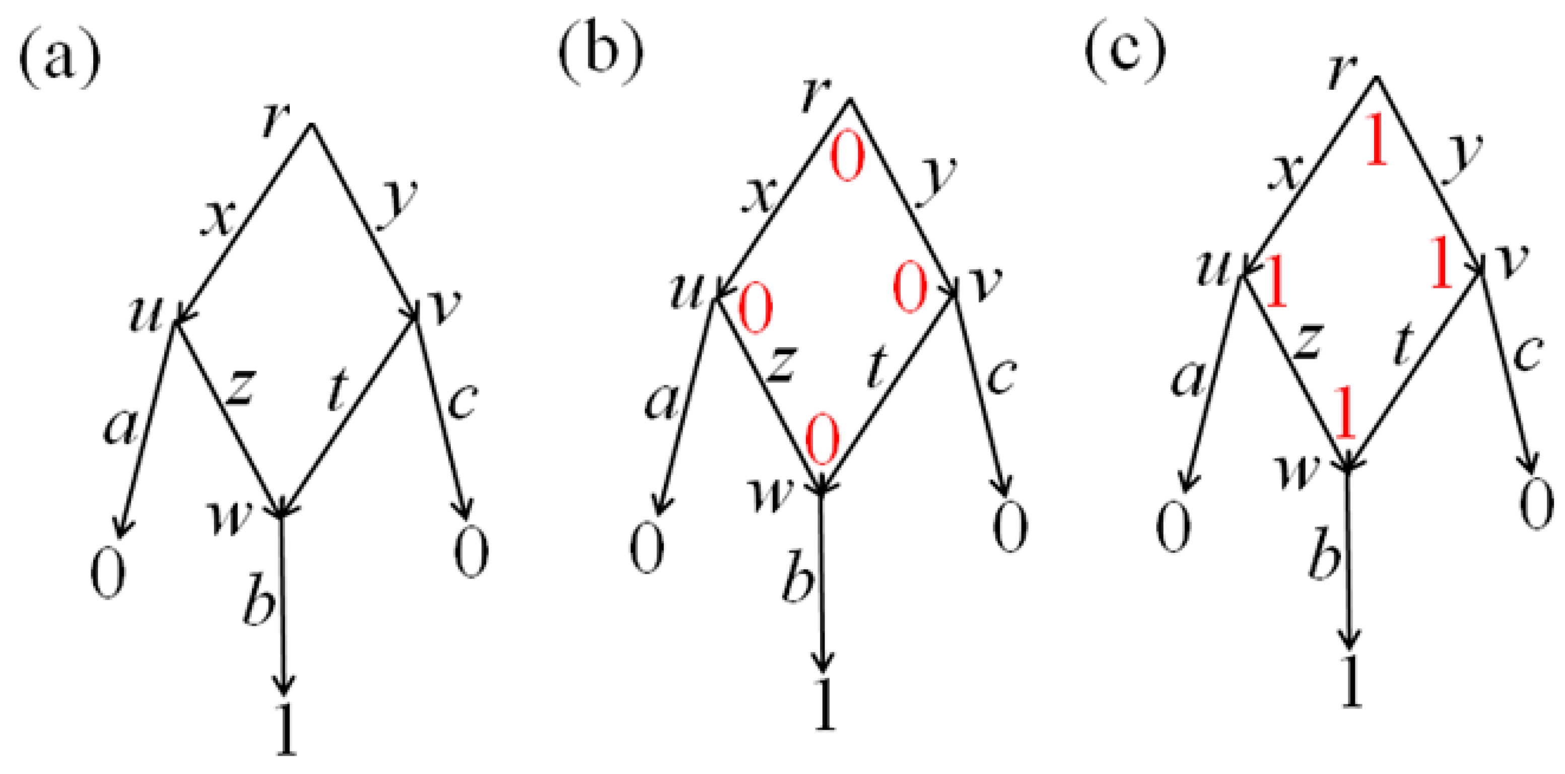
Simple algorithm. Let us provide a network and, in its leaves, structures (matchings) with equal content. Then, for each potential edge p ∈ M (i.e., a pair of extremities in the set M) in every leaf v of this network there is a binary p-label (p-attribute), which indicates whether the extremities composing p in the matching of this v are joined (1) or cut (0). In other words, label 1 indicates the presence of an edge p in the v-matching, and 0 indicates its absence in the v-matching. We perform reconstruction along the network independently for each p-attribute using the algorithm from Section 2. A pair of extremities that are not joined in any leaf is reconstructed trivially. A potential edge p ∈ M is said to be nontrivial if the extremities that constitute p are joined in at least one leaf of the initial data, including joins by a loop.

Then, in each node v of the network there is defined a set of all p-reconstructions, which will define a pseudo-structure G consisting of edges p ∈ M with p-label 1 in v. In other words, in each node v of the network, the p-labels at the leaves (for all p in the aggregate) uniquely define their own pseudo-structure G_v; thus, they define an arrangement G of pseudo-structures along the network. In the case of p-label 1, we will write p ∈ G_v, and in the case of p-label 0 we will write p ∉ G_v.

By successively examining extremities x ∈ M in all nodes v of the network in an arbitrary order, we remove all x-edges from the v-pseudo-structures composing G that are incidental to more than one other x-edge. Thus, we obtain a final arrangement R of structures. We call the described algorithm simple. Despite its simplicity, it has a surprising property formulated in Theorem 2.

Modified algorithm. Often one searches for an arrangement of matchings whose total number of edges (over all its matchings) is large. For this purpose, below we propose an algorithm of reasonable complexity for real computations, which we will call a modified algorithm. We cannot prove that it maximizes the specified number of edges while preserving the multiplicative exactness estimate given in Theorem 2, although our practical use of this algorithm indicates that these properties are present. The modified algorithm consists of the simple algorithm as its first stage, and two subsequent stages. We denote by R the result of the first stage, an arrangement along a given network of matchings in M. Let us describe the second and third stages of the modified algorithm.

Second stage. We successively examine all nontrivial potential edges p ∈ M. An arrangement R₁ of matchings along a given network is obtained from an arrangement R of matchings in the following way. In each non-leaf node v, we add the edge p to R(v) if p ∈ G_v, or remove it if p ∉ G_v. In the resulting arrangement of pseudo-structures, we remove the original x-edge (not p itself) if at some extremity x ∈ M the incidence is violated; thus we obtain R₁. For the current p, we compute the first score c(R) − c(R₁), where c(·) is the cost of the arrangement.

When computing the second score, another arrangement—R₁—is obtained from R as follows. We add or remove an edge p ∈ M in matchings from R according to the conditionally minimal p-attribute, which in each node v is preliminarily labeled by 0 if there is an edge in R(v) that is incidental to the extremity of the current potential edge p. Compute the second score c(R) − c(R₁).

Both these arrangements—R₁(p), p ∈ M—are used to compute the maxima over p of the first and second scores. Let the first of them be attained at an edge p′ with value a, and the maximum of the second score be attained at an edge p″ with value b. If a ≥ 0 and a > b, we replace R(p′) with R₁(p′), and on the other edges R remains unchanged. If a = 0, the replacement is made if it strictly reduces the total number X(R) of connected components (we say, components) in all structures of the arrangement R relative to R₁. If b ≥ 0 and a ≤ b, then we replace R(p″) with R₁(p″) with the same stipulation if b = 0; on the other edges, R is unchanged. Otherwise, R₁ = R. Obviously, the cost c(·) does not increase when passing to R₁.

We repeat this iteration while one of the two things is realized: the cost c(R) or the total number of components X(R) strictly decreases when passing to the arrangement R₁.

Third stage of the modified algorithm is descent to a local minimum, as described in the work presented in [28] (Section 7). Let us recall how this descent is performed. For each node v of a given network and for each nontrivial potential edge p ∈ M, denote by p_no the cost c₂ or c₃ (depending on whether p is a loop) of removing p multiplied by the number A of network edges entering v at the beginnings of which p is present, summed with the cost c₁ or c₄ (with the same dependence) of adding p multiplied by the number B of network edges leaving v at the ends of which p is present. Thus, p_no = (c₂ or c₃)·A + (c₁ or c₄)·B. Similarly, let p_yes denote the cost c₁ or c₄ of adding p multiplied by the number of network edges entering v at whose beginnings p is absent, summed with the cost c₂ or c₃ of removing p multiplied by the number of network edges leaving v at whose ends p is absent. For each node v of the network, to each nontrivial potential edge p ∈ M we assign the weight p_yes − p_no, and for v we construct a minimum weighted matching in M with these weights, which we assign to v. In the other nodes of the network, we keep the same matchings, thus, obtaining an arrangement R₁(v). Let the difference, c(R) − c(R₁(v)), which is maximal over all nodes v be attained at a node v′. If this difference is strictly positive, we replace the arrangement R with R₁.

We repeat this iteration while c(R) − c(R₁(v)) is strictly positive.

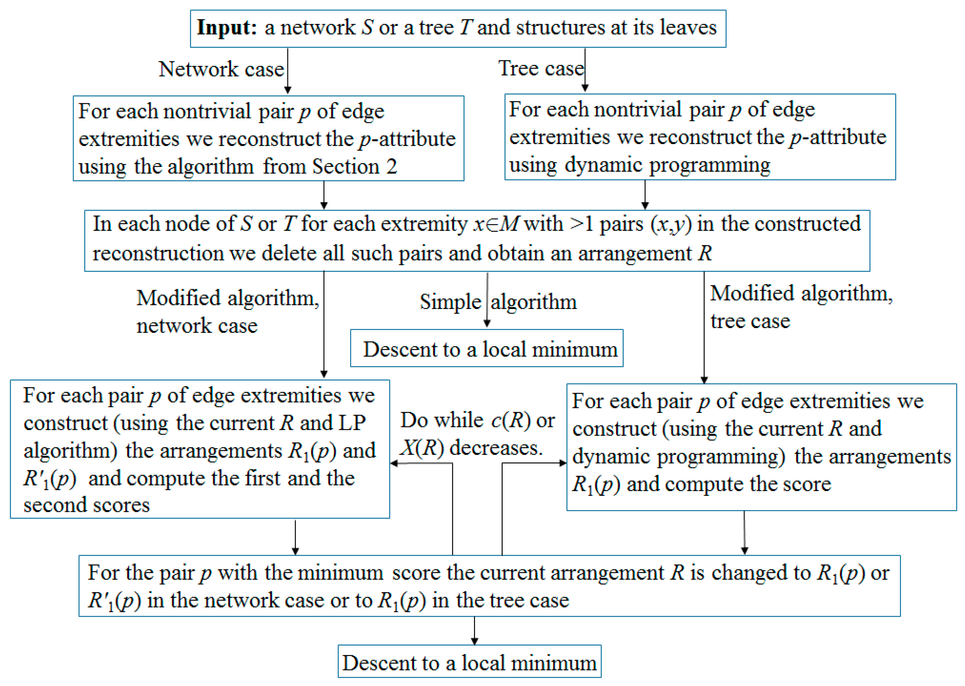
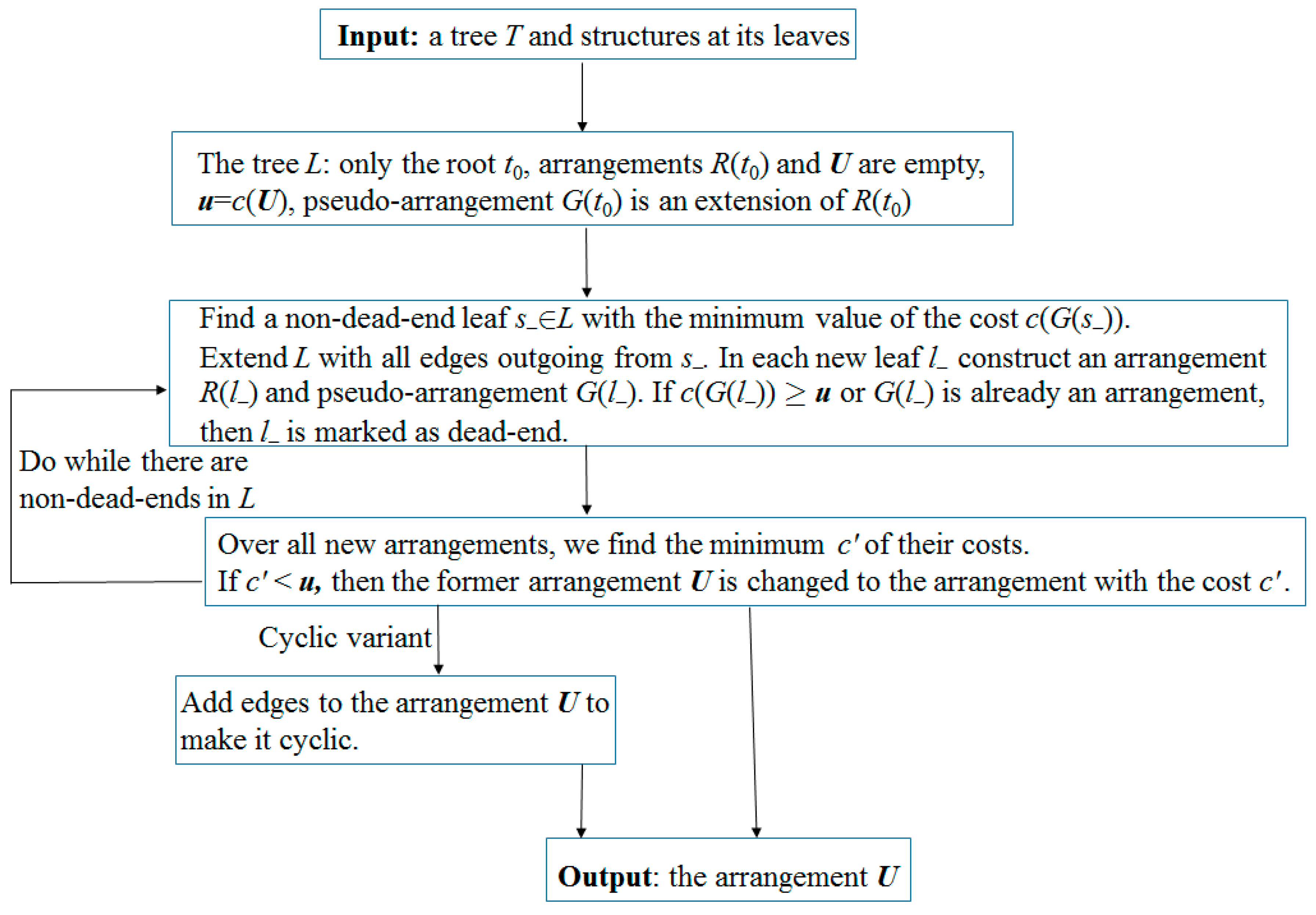
Remark 3.

According to our computational experience, if the initial network is a tree, then it is more efficient to use dynamic programming instead of the above LP algorithm. Namely, the reconstruction of each p-attribute is performed by induction from leaves to root, resulting in pseudo-structures at all nodes. By removing unnecessary edges in them, we complete the simple algorithm. In the second step of the modified algorithm, instead of two p-scores, we by induction compute one score c(R) − c(R₁). The arrangement R₁ has the minimum cost among all arrangements that are obtained from R in the following way. In each node of the tree, one of the three rearrangements of matchings is independently performed: change nothing (empty rearrangement), remove the edge p (if it existed); or add it (if it did not exist), in which case we remove other edges incident to p. This is done by leaf-to-root induction: in every next node v, for each of its above rearrangements, in each of its child nodes v₁ we choose the one of the above rearrangements in which c(v,v₁) + c(v₁) is minimal. Here, the first term is the distance between matchings at v and v₁, and the second is the minimum cost of rearrangements along the subtree with root v₁, which is known by the induction assumption. Having reached the root r of the tree, we choose a rearrangement in it with the smallest value of ${\displaystyle \sum _{i}c(r,v_i)+c(v_i)}$, where the v_i are all child nodes of r. Then, by backward pass, we construct the arrangement R₁ itself. The flow chart of the algorithm is shown in Figure 2.

3.3. Exactness of the Algorithm

For an arrangement of pseudo-structures along a given network, an event on an edge e of the network is that some potential edge p ∈ M enters the pseudo-structure assigned to one endpoint of e and does not enter the pseudo-structure assigned to the other endpoint of e. Recall that an edge p corresponds to a join of its extremities in the corresponding structure. An event occurs as a result of one of the four operations on the pseudo-structure, and the cost of the corresponding operation is considered to be the cost of the event. These operations are a join of extremities of pseudo-structures (with cost c₄ if they are extremities of the same edge, and c₁ otherwise) and a cut of extremities of pseudo-structures (with cost c₃ if they are extremities of the same edge, and c₂ otherwise).

The cost of an arrangement of pseudo-structures (in particular, structures) is the sum of costs of all events on all edges of the network. On any edge e of the network, this sum is defined in two more equivalent ways; below, we use either of them without specifying. First, as the sum of costs c₁, c₂, c₃, and c₄ of SCJ operations that transform a pseudo-structure at the beginning of e into a pseudo-structure at the end of e (see Section 3.1); the definition for structures is just the same. Second, as the sum over all edges p ∈ M of the costs of transitions along an edge e of the network between p-labels on its extremities, which (in our case) result from the reconstruction of p-labels at the leaves.

Denote by c_min the minimum of costs of the operations and by c_max the maximum of these costs. Costs of all operations can be considered as integers, which would not lessen the generality of our presentation.

Theorem 2.

(a) The simple and modified algorithms admit a multiplicative error of at most c_max/c_min. In particular, both algorithms are exact under equal costs of operations. The runtime of the simple algorithm is of the order of n·s·L, where n is the cardinality of the set M, s is the size of the given network, and L is the time required to solve the above-mentioned linear programming problem, whose size depends linearly on the size of the network. The runtime of the second stage of the modified algorithm is of the order Cns(L + s) + (ns)²·L + ns³, where C is the cost of the minimum arrangement of structures along the network. The runtime of the third stage of the modified algorithm is of the order n²·(s + log n)·sC.

(b) If a given network is a tree, then both algorithms are also exact in the case c₁ = c₄, c₂ = c₃, c₂ ≥ c₁.

Proof. 

(a) In the simple algorithm, the number of events in its final arrangement R of structures is not greater than the number of events in the arrangement G of pseudo-structures, since at each iteration the number k of events on an arbitrary network edge e with some extremity x ∈ M does not increase. Indeed, if at both ends of e in their pseudo-structures the extremity x is incident to more than one other extremity, then after an iteration all these edges are missing. If at both ends of e the extremity x is incidental to no more than one extremity, then the same edges remain at the ends. If there is, at most, one x-edge at one end of e and strictly more than one at the other end, then all x-edges at the second end are removed, and k does not increase. Let k and k′ be the numbers of events in the arrangements G and R, respectively; then k ≥ k′.

The total cost of events in G is c(G) ≥ c_min·k, and for R it is c(R) ≤ c_max·k′. The cost c(G) is minimal among the costs of all arrangements of pseudo-structures. Therefore, for the cost C of the minimal arrangement of structures, we have c(G) ≤ C. Therefore, c(R)/C ≤ c_max/c_min. At the second and third stages of the modified algorithm, the arrangement cost does not increase. Hence we obtain the first claim of the theorem. The estimate for the runtime of the simple algorithm follows from its description.

At each iteration in the second and third stages of the modified algorithm, we have c(R₁) < c(R) or X(R₁) < X(R). In any structure, the number of components takes a value from 1 to the integer n/2. Hence, for the order of the runtime of the second stage, we obtain an upper estimate (C + ns)·ns·(L + s), since this estimate is c(R) + ns/2 = C + ns/2 multiplied by the estimate for the runtime of one iteration, which for each nontrivial pair p (their number being of the order ns) includes specifying the data of the LP problem, solving the problem, and processing the result. The estimate for the runtime of the third stage follows from the estimate for the time to construct a minimal matching in any graph with n′ vertices and m edges, which is of the order of n′·m + (n′)²·log(n′), [42] (Chapter 11).

(b) In the simple algorithm, first an arrangement G of pseudo-structures is formed as the union of minimal arrangements of p-labels over all p ∈ M and all nodes v of the network. Then, as a result of cuts and joins, an arrangement R of structures is output. In the simple algorithm executed on a tree, after every next arrangement, the number of cut events (i.e., those with costs c₂ or c₃) does not increase. Indeed, this number can only increase (and only from 0 to 1) on an edge e of the tree at the beginning of which some extremity x ∈ M is incident to exactly one extremity y and at the end x is incident to more than one extremity, possibly including y. Consider the edge e and the component K in the set consisting of the node v of the original tree in the matchings of which the extremity x is incident to more than one extremity y; the edge e enters K (from the root side). Only e enters K; leaves of the tree do not belong to K. Iteration on edges that connect nodes from K will not increase the number of events. On an edge leaving K (there are at least 2 such edges), the number of x-cut events strictly decreases. Thus, the simple algorithm does not increase the number of cuts with cost c₂ = c₃; assume that the algorithm reduces this number by k₂ ≥ 0.

By part (a) of Theorem 2, the simple algorithm does not increase the number of all events. Therefore, for the number k₁ by which the number of joins with cost c₁ = c₄ is increased, we have k₁ ≤ k₂. The condition c₂ ≥ c₁ implies that the simple algorithm changes c(G) to −c₂·k₂ + c₁·k₁ ≤ 0; i.e., c(G) ≥ c(R) and c(G) = c(R), since c(G) is the minimum cost. Hence, the algorithm outputs an arrangement R of structures whose cost c(R) is minimal even among all arrangements of pseudo-structures. Thus, the simple algorithm is exact, and then the modified algorithm is exact too. □

Remark 4.

For the cyclic reconstruction problem we apply the following algorithm, which we will call cyclic. It differs from the modified algorithm only in the third stage, which we will now call the cyclic descent. Namely, instead of a minimum matching, the algorithm constructs a minimum complete matching and hence the structure at node v’ is always replaced by a cyclic structure. The difference c(R) − c(R₁) can be negative if the structure in v’ was not cyclic before the replacement. The cyclic algorithm is heuristic; for it, the authors did not succeed in proving the error estimate formulated in Theorem 2.

Remark 5.

There is another possible approach in the problem of structure reconstruction. To each nontrivial potential edge p∈ M we associate a set of the same variables at the network nodes and edges as in the LP-problem of Section 2.2, i.e., x_p at the network nodes and z_p at the edges. In each leaf, x_p = 1 if the edge p belongs to the matching, and x_p = 0 otherwise. For each p, we impose the corresponding constraints: all variables are in [0, 1], x_p + y_p + z_p ≤ 2, x_p + z_p ≥ y_p, y_p + z_p ≥ x_p, and x_p + y_p ≥ z_p. We impose new constraints: for each non-leaf node of the network and for each extremity x∈ M we have ${\displaystyle \sum _{p=(x,y)}{x}_p\le 1}$. The objective function is the sum of the objective functions of the LP problem mentioned above:

$$F=\frac{1}{2}{\displaystyle \sum _p{\displaystyle \sum _{z=(x_p,y_p)}(c_{10}(z_p+x_p-y_p)+c_{01}(z_p+y_p-x_p))}\to \min }$$

(2)

If the solution of this LP problem is Boolean, then at each node of the network it defines a matching in M. However, the solution of this LP problem need not necessarily be Boolean, and then the coordinates of the solution can be viewed as probabilities for the edge p to enter the desired matching.

3.4. Example of the Algorithm Operation

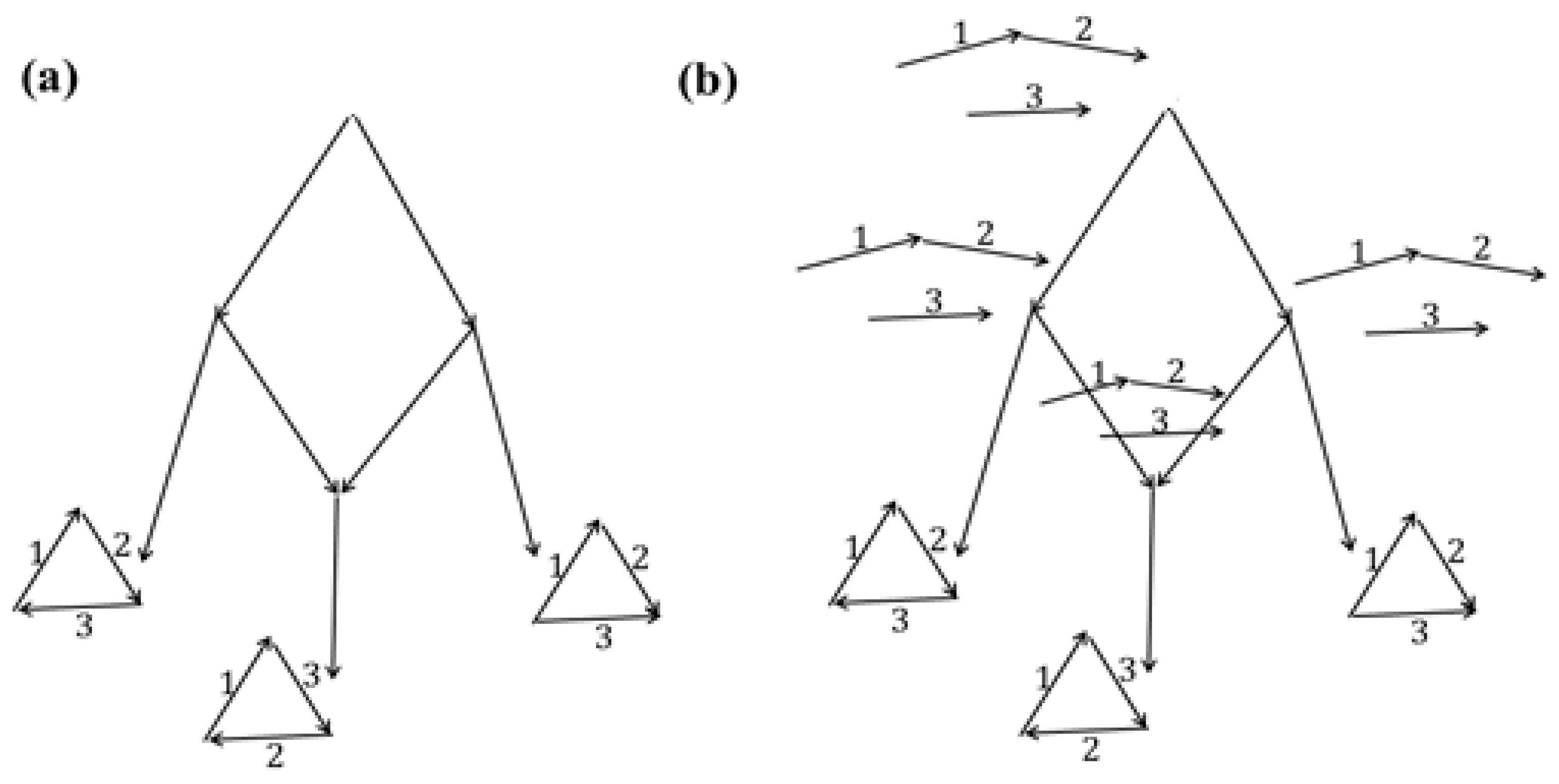
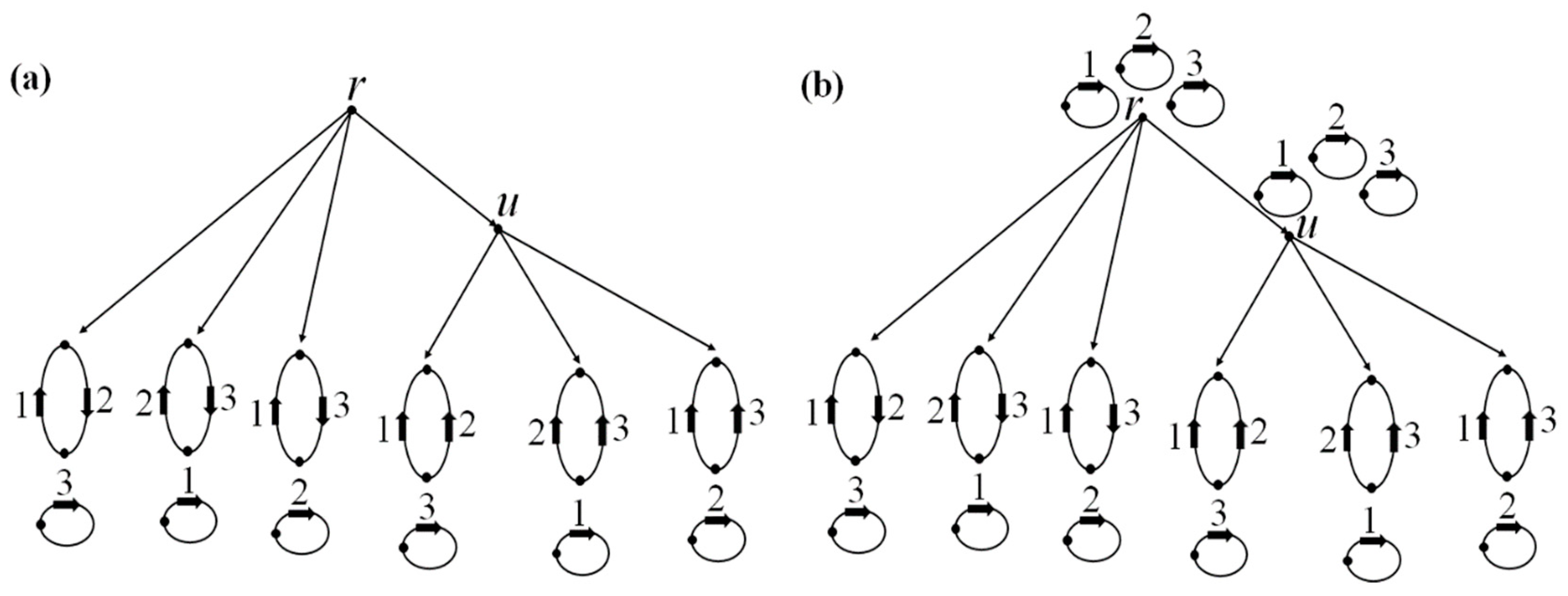
Consider the network with the initial data shown in its leaves in Figure 3a. Let c₁ = c₂ = c₃ = c₄ = 1. Applying the algorithm of Section 2 to the eight joins present in the leaves, we obtain that only the edge (1₂,2₁) is present in the arrangement G of pseudo-structures shown at the non-leaf nodes of the network. Thus, G is already an arrangement of structures, which is shown in Figure 3b and is minimal. Its cost is 8.

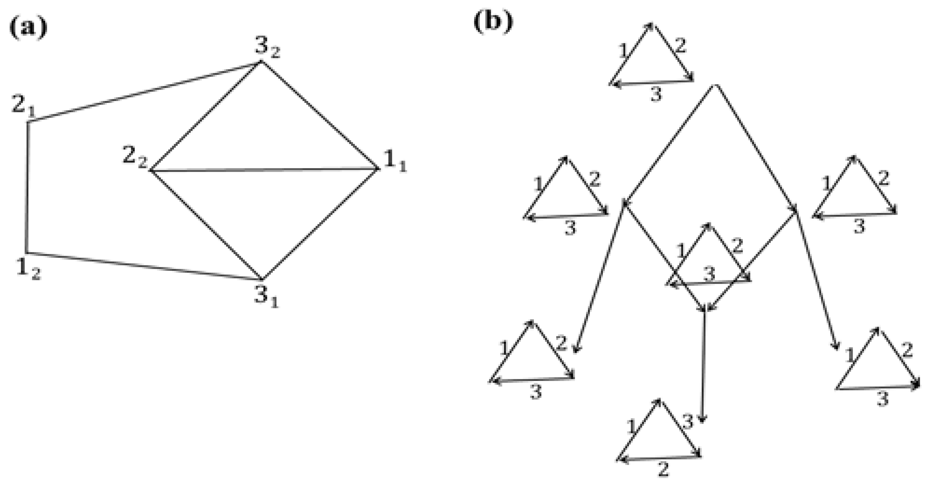
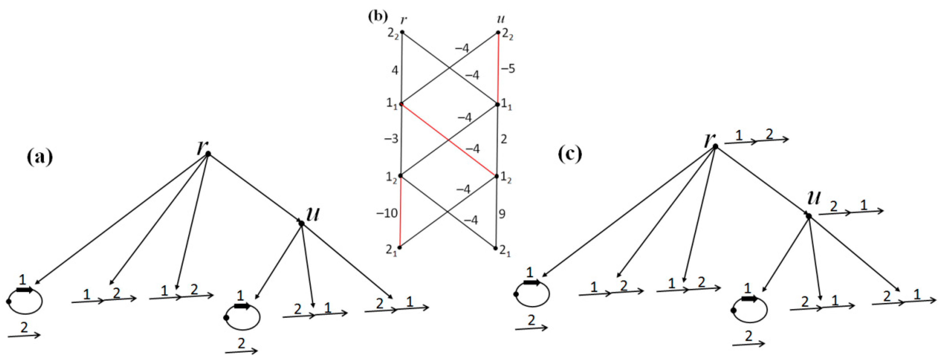
Now let c₁ = c₄ = 6 and c₂ = c₃ = 1 (i.e., let a join of extremities have cost 6 and a cut of extremities have cost 1). The arrangement G of pseudo-structures is the same at all nodes and is shown in Figure 4a. Let us apply the modified algorithm. Let the order of examining the extremities x at the first stage be 2₁, 3₁, 3₂ (here the final result does not depend on the choice of the order). After the first step, only the edge (1₁,2₂) remains in G. At the second stage and at the first iteration, the maximum of the two scores (the first one) attains the maximum of eleven on the edge (1₂,2₁), at the second iteration it attains the maximum of 0 on the edge (1₁,3₂), and at the third iteration it attains the maximum of four on the edge (2₂,3₁). After adding these edges and removing the edge (1₁,2₂), we obtain the resulting arrangement, Figure 4b. This arrangement is minimal with cost 35.

4. Reconstruction of Structures along a Tree

4.1. Problem Setting

We again consider the same problem of reconstructing structures, now not along a network, but along a given tree T, which in the general case is nonbinary (sometimes referred to as polytomous). As in Section 3, we first ensure equal content of structures defined at leaves, and therefore, equal content of all desired structures at non-leaf nodes of the tree. As above, the reconstruction problem reduces to constructing in each non-leaf node of the tree a matching on the same set M of names of extremities of all edges at the leaves. In contrast to Theorem 2, we describe here another algorithm for solving this problem based on dynamic programming, which turns out to be exact if a natural condition formulated below is satisfied. It is important that the runtime of the algorithm is estimated by a third-order quantity with respect to the size of the original problem multiplied by the size of the auxiliary tree, which usually takes small values.

For an extremity x ∈ M, by an x-arrangement we call an unambiguous assignment of at most one edge p ∈ M incident to x (in the cyclic variant, exactly one edge) to each node of a given tree T. An x-arrangement is a particular case of an arrangement of matchings. The cost of an x-arrangement is defined to be its cost as of an arrangement of matchings; in this case, only edges incident to x are left in the leaves of T.

An x-arrangement with a minimum cost is constructed by induction. At leaves, an x-arrangement is given by an edge with which the extremity x is joined, or by an empty set. An x-edge is defined to be either an edge in M with extremity x or the symbol Ø of the empty set. For a fixed extremity x ∈ M, we examine the nodes of T from leaves to the root; at each node v and for each potential x-edge p in v, we compute the function c(v,p) = å_v′ c(v′). Here, c(v,v′,q) is the number of events on the edge (v,v′) if q is assigned to a child node v′ of the tree, c(v′,q) is the minimum cost of an x-arrangement over a subtree with root v′ in which the x-arrangement is q, and c(v′) = min_q c(v,v′,q) + c(v′,q). Let the minimum of c(v′) be attained at q(p); c(v,p) and q(p) are stored in v. At the root r ∈ T, we choose the x-edge with the minimum value of c(r,p) over p, and then perform the backward pass of dynamic programming. The resulting x-arrangement has the minimum cost among all x-arrangements and is said to be minimal.

Let an arrangement R of matchings along T be given. Then, a conditionally minimal x-arrangement R′ along T extending R is defined as the minimum-cost x-arrangement among all x-arrangements containing all x-edges from R and not containing x-edges whose other extremity is incident to an edge from R. It is constructed by dynamic programming similarly to the preceding algorithm. Note that all x-edges from R are included in R′; in this sense, R′ is an extension of R.

On the other hand, let us be given an arrangement R of matchings along T and a set X ⊆ M. By a conditionally minimal extension G of the arrangement R with respect to X, we call an extension of R by edges of conditionally minimal arrangements of p-labels along nontrivial potential edges p ∈ M one or both extremities of which are not contained in X. The condition is that a p-label at node v ∈ T is 1 if p ∈ R(v), and is 0 if p is incident to an edge q ∈ R(v), q ≠ p. Unlike R, G is an arrangement of pseudo-structures along T, and to construct it, we use the algorithm provided in Section 2.2; see also Remark 1 in Section 2.3. Obviously, R ⊆ G.

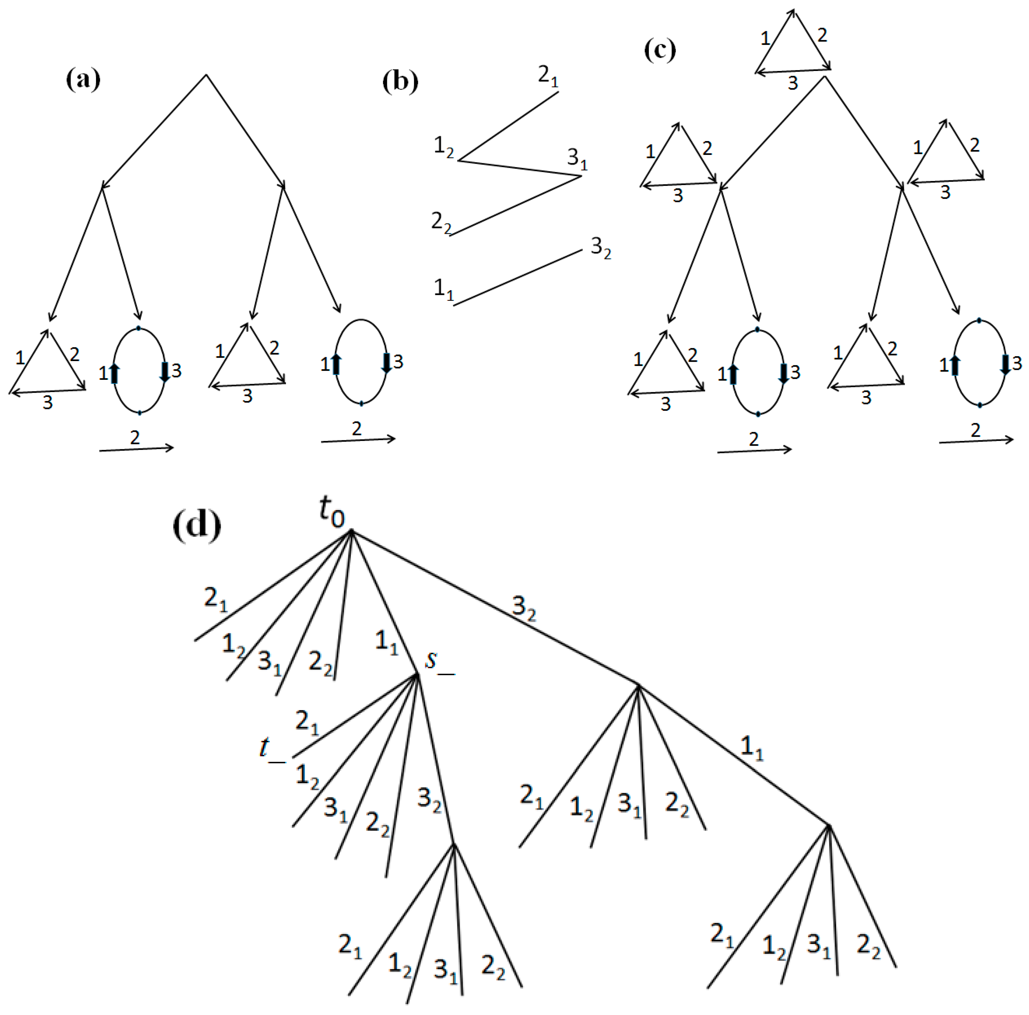
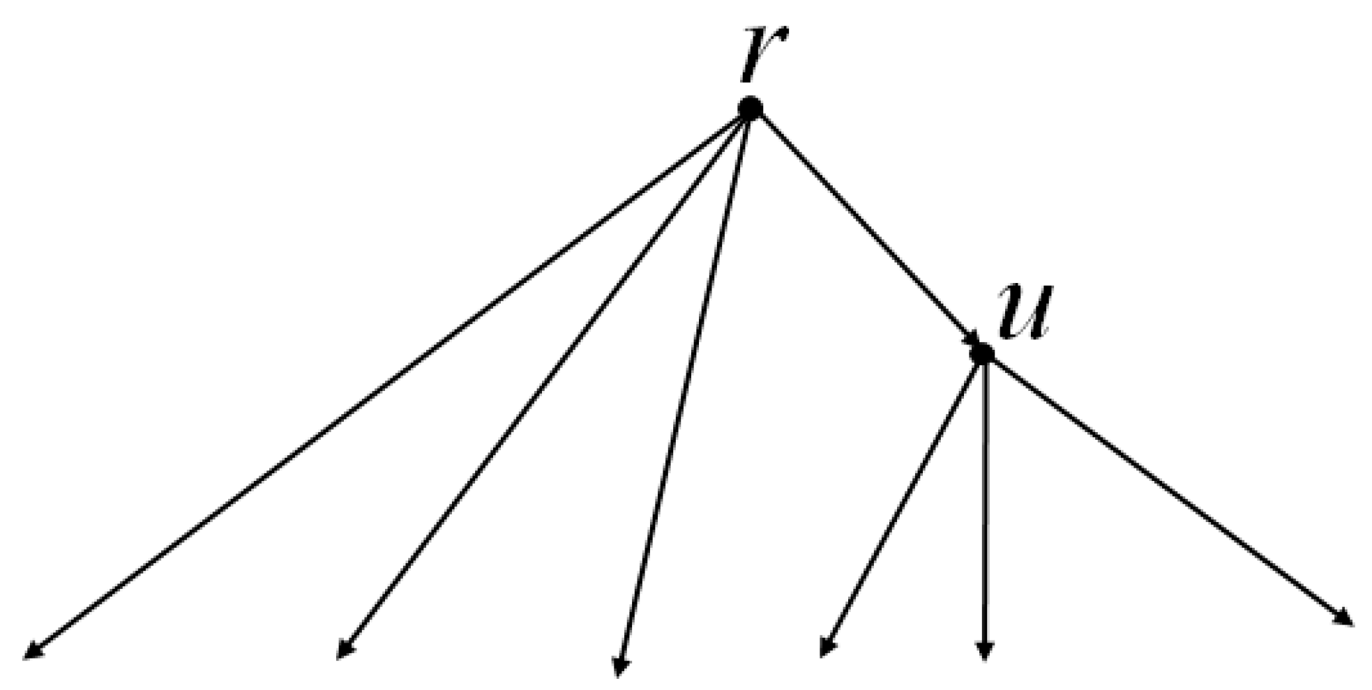
We will need a separate auxiliary tree L with root t₀, which represents variants of possible extensions of the empty arrangement along the tree T. A path in L from the root to a leaf shows one variant of such a consecutive extension of the empty arrangement. Throughout what follows, by a path in L we mean a path from t₀, which is not specified explicitly. For each edge l ∈ L, we denote its beginning by l₊ and its end by l₋. Each node l_– will be assigned with an extremity x ∈ M, which we denote by x(l). Moreover, in any path to a node l_– ∈ L, the extremity x(l) occurs only once, at the very end. From any non-leaf node in L there emerges edges uniquely labeled by x(l), for every x ∈ M that does not occur in a path to l₊, see Figure 6d.

4.2. Description of the Algorithm

Recall that the cost of an arrangement R of structures or an arrangement G of pseudo-structures along a tree T is denoted by c(R) and c(G).

Before each iteration, the algorithm has a current tree L with some leaves marked as dead-end leaves. Moreover, each node l₋ ∈ L is unambiguously assigned with an arrangement R of matchings and an arrangement G of pseudo-structures, both along the initial tree T (in the leaves of which, initial structures are still fixed; they are also pseudo-structures). Even before each iteration, the algorithm has an arrangement U of matchings at non-leaf nodes in T (at the leaves it coincides with the original structures) and a cost u of this arrangement. At each iteration except the last one, the tree L is continued “downwards”, see the first example in Section 4.4.

Before the first iteration, L consists of a single non-dead-end root t₀ ∈ L, the arrangement R(t₀) along T consists of empty matchings (at leaves there are original matchings), G(t₀) is the conditionally minimal extension of the arrangement R(t₀) with respect to the empty set, i.e., the union of the minimal arrangements of all p-attributes. Finally, U is the empty arrangement (except for the leaves, which contain the original matchings), and u = c(U).

Let us describe the iteration itself. Find a non-dead-end leaf s₋ ∈ L (at the first iteration, s₋ = t₀) with the minimum (over all non-dead-end leaves) value of the cost c(G(s₋)). Extend L with all edges l outgoing from s₋ with all labels x(l) that do not occur on the path to s_–. For each added edge l ∈ L, construct an arrangement R(l₋) of matchings and an arrangement G(l₋) of pseudo-structures, both along T, see the first example in Section 4.4:

(1)

R(l₋) is the union of the arrangement R(s₋) and the conditionally minimal x(l)-arrangement that extends R(s₋), where l₊ = s₋;

(2)

G(l₋) is the conditionally minimal extension of the already obtained arrangement R(l₋) with respect to X(l) ⊆ M. Here, X(l) is the set of extremities that occur on the path to l₋.

If c(G(l₋)) ≥ u or G(l₋) is already an arrangement of matchings, then l₋ is marked as dead-end. Over all added nodes l₋ (outgoing from s₋), we find the minimum c′ of costs c(R(l₋)), and if G(l_–) consists of structures, then including also the costs c(G(l₋)). Let c₋ be attained at t_–. If c′ < u, then the former price u is changed to c’ and the former arrangement U is changed to either R(t₋) or G(t₋) (according to which of them the minimum is attained). The ambiguity that may arise in this case is eliminated by using a random choice, which is the end of the iteration.

The iterations are performed until all the leaves in the next tree L are marked as dead-end. Then, as the final arrangement along T, the algorithm outputs the current arrangement U and its cost u.

The cyclic variant of the algorithm contains an additional step executed after all the above iterations. Namely, if the final arrangement is not cyclic, then, by examining the extremities x ∈ M in an arbitrary order, we extend the current arrangement by a conditionally minimal x-arrangement with the following condition: at each node v ∈ T the matching property is not violated, and the extremity x enters the matching. This condition can always be ensured, since the current arrangement at each node covers an even number of extremities and n = |M| is an even number. Indeed, if an x-edge is missing, it can be chosen without violating the matching property.

The flow chart of the algorithm is shown in Figure 5.

4.3. Justification of the Algorithm

The following property is often fulfilled in structure reconstruction problems arising, for example, in evolutionary genomics, cell type construction, etc.

Extremity enumeration property. There exists a bijective enumeration of all extremities r₁, …, r_n in M for which the arrangement R_n of matchings is minimal and for which R₁ is the union of R(t₀) and the unique minimal r₁-arrangement, R₂ is the union of R₁ and the unique conditionally minimal r₂-arrangement extending R₁, etc. Thus, each R_i+1 is an extension of the preceding R_i.

Both the fulfillment and non-fulfillment of the enumeration property depend on a particular enumeration, as can be seen in the examples in Section 4.4. In the first one, this property is satisfied for the enumeration of extremities 2₁2₂3₁3₂1₁1₂ and is not satisfied for the enumeration 1₁1₂2₁2₂3₁3₂, since in the latter case the uniqueness is violated at R₂. In the second example in Section 4.4, any enumeration obeys the enumeration property. We emphasize that the algorithm presented below does not use any initial enumeration of extremities in M.

Theorem 3.

If the extremity enumeration property is fulfilled in the reconstruction problem, then the above algorithm produces an exact solution. Its runtime is of the order of n·s²·l, where n is the cardinality of the set M, s is the size of the tree T, and l is the size of the resulting tree L.

Proof. 

Let r₁, …, r_i, …, r_n be an enumeration of all extremities satisfying the above property, and let R_i be a current arrangement of matchings. In the final tree L, consider a path with labels r₁, r₂, …, r_i from the root to a dead-end leaf. By induction, due to the uniqueness of conditionally minimal r_i-arrangements, we have R(r_i) = R_i.

Let us check that c(G(r_i)) ≤ c(R_n). Consider potential edges p = (x,y) ∈ M for which x,y ∈ X(r_i) is satisfied; denote the set of such edges by I, and denote its complement by I’. Then, we have $c(G(r_i))={\displaystyle \sum _{p\in I}c({S^{\prime }}_p)+}{\displaystyle \sum _{p\in I^{\prime }}c({S^{\prime }}_p)}$ and $c(R_n)={\displaystyle \sum _{p\in I}c(S_p)+}{\displaystyle \sum _{p\in I^{\prime }}c(S_p)}$, where S′_p and S_p are the arrangements of p-labels induced by G(r_i) and R_n, respectively. The arrangements G(r_i) and R_n are obtained from R(r_i) = R_i by adding the edges p ∈ I’. Therefore, G(r_i) and R_n differ at edges from I’ only; i.e., the first terms in these sums are the same. Since in G(r_i) for p ∈ I’ every arrangement of p-labels is minimal, we obtain c(G(r_i)) ≤ c(R_n).

Consider two cases in which r_i is a dead-end leaf.

Let G(r_i) be an arrangement of structures. Then, c(G(r_i)) = c(R_n) = C, where C is the minimum cost of all arrangements of structures along T. For edges from r_i–1 (from t₀ for i = 1) we have c′ = C, and if c′ < u, then at this iteration we let u = C and U = G(r_i), and at the next iterations these u and U cannot change. The algorithm outputs the final arrangement U with cost C. If C = u, then the algorithm had obtained the final arrangement U with cost C at the previous iteration.

Now, let the first case c(G(r_i)) ≥ u, occur, where u is computed at the previous iteration. Then, c(G(r_i)) ≥ u ≥ c(R_n) and c(G(r_i)) = c(R_n) = C = u = c(U). Therefore, the algorithm does not change u and U at this and the next iterations, outputting the final arrangement U with cost C.

The estimate for the runtime of our algorithm follows from the fact that for each node in L, the auxiliary dynamic programming algorithm that constructs an arrangement of p-labels is executed of the order of ns times, and each time its runtime is of the order of s. □

4.4. Examples of the Algorithm Operation

First example. Consider a tree T with the structures at its leaves shown in Figure 6a. Let costs of joins be c₁ = c₄ = 3 and costs of cuts be c₂ = c₃ = 2. First, the tree L consists of the root t₀. The arrangement R(t₀) of matchings is the same at all non-leaf nodes in T (empty one, except for the leaves), and u = c(U) = 30. And the arrangement G(t₀) of pseudo-structures with cost 12 is the same at all non-leaf nodes in T (the original one at the leaves) and is shown in Figure 6b.

Let us extend the tree L with edges outgoing from t₀; then we obtain that for the edge l with end l_– = 2₁ we have the following: R(2₁) = (1₂,2₁) is the same at all non-leaf nodes in T, c(R(2₁)) = 28, and similarly the arrangement G(2₁) is the same at all non-leaf nodes in T and coincides at them with the matching {(2₂,3₁), (1₂,2₁), (1₁,3₂)} shown in Figure 6c. Therefore, the node 2₁ is marked as dead-end. Here, c(G(2₁)) = 14. For other new edges l ∈ L, we obtain costs of the structures R(l_–) and G(l_–) not less than 14: R(1₂) = (1₂,2₁) or R(1₂) = (1₂,3₁), c(R(1₂)) = 28, and G(1₂) = {(2₂,3₁),(1₂,2₁),(1₁,3₂)} with c(G(1₂)) = 14 or G(1₂) = {(1₁,3₂),(1₂,2₁)} with c(G(1₂)) = 16. Next, R(3₁) = (1₂,3₁) or R(3₁) = (2₂,3₁), in both cases c(R(3₁)) = 28; and G(3₁) = G(1₂). Then, R(2₂) = (2₂,3₁), c(R(2₂)) = 28, G(2₂) = G(2₁); and R(1₁) = (1₁,3₂), c(R(1₁)) = 18, G(1₁) = G(t₀); finally, R(3₂) = R(1₁), G(3₂) = G(t₀). Ends of the edges from t₀ are dead-end except for 1₁ and 3₂. Therefore, c’ = 14 and t_– = 2₁; hence we obtain U = G(2₁) and u = 14.

Further extension of L does not change the values of U and u: for instance, for the end of the path t₀1₁1₂ (l_– = 1₂) we have R(1₂) = {(1₁,3₂), (1₂,2₁)} at all non-leaf nodes v ∈ T, or alternatively R(1₂) = {(1₁,3₂), (1₂,3₁)}; both arrangements have cost 16. Next, G(1₂) = {(2₂,3₁), (1₂,2₁), (1₁,3₂)} at non-leaf nodes v ∈ T, or alternatively G(1₂) = {(1₁,3₂), (1₂,3₁)}; these are arrangements with costs 14 and 16, respectively. For other edges l ∈ L from the node 1₁ of the tree L, we obtain that the costs of arrangements of the structures R(l_–) and G(l_–) are at least 14: R(2₁) = {(1₁,3₂), (1₂,2₁)}, c(R(2₁)) = 16, G(2₁) = {(2₂,3₁), (1₂,2₁), (1₁,3₂)}, c(G(2₁)) = 14; R(3₁) = {(1₁,3₂), (1₂,3₁)} or {(1₁,3₂), (2₂,3₁)}, c(R(3₁)) = 16, G(3₁) = G(1₂); R(2₂) = {(1₁,3₂), (2₂,3₁)}, c(R(2₂)) = 16, G(2₂) = G(2₁); R(3₂) = (1₁,3₂), c(R(3₂)) = 18, G(3₂) = G(t₀). Ends of the edges from 1₁ are marked as dead-ends except for 3₂. Thus, the algorithm outputs the same U as an arrangement and the same u as its cost until all nodes in a current L become dead-ends. Such a final tree is shown in Figure 6d, in which all leaves correspond to the extremities 2₁, 1₂, 3₁, 2₂ in M. The algorithm outputs the previously obtained U and u as the final ones.

It is easy to directly check that the arrangement U has the minimum cost u = 14, i.e., it is minimal.

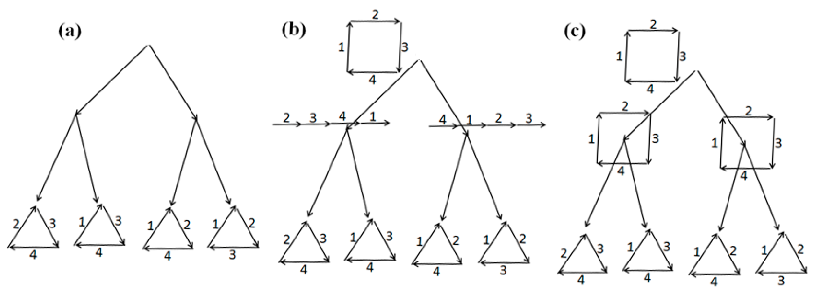
Second example. Consider a tree T with the structures at its leaves shown in Figure 7a; edges missing at the leaves are replaced with loops, which is not shown in this figure. Let the operation costs be the same as in the first example. If a nontrivial edge p ∈ M is present in exactly one leaf, then p-labels at all non-leaf nodes are 0. If p is present in exactly two neighboring leaves, then the p-label at two non-leaf nodes is 1 and at the third is 0. If p is present in exactly two non-neighboring leaves, then the p-label is 1 at all non-leaf nodes. Hence we see that the arrangement G(t₀) of pseudo-structures consists of structures, and the algorithm outputs it as the final one, Figure 7b. The resulting tree L consists of a single dead-end root t₀.

In the cyclic version of the algorithm with the same costs, the additional step adds one edge at each of the two non-root nodes. The final arrangement is shown in Figure 7c.

5. Polynomial Algorithm for Reconstruction of Structures on a Two-Star Polytomous Tree

5.1. Problem Setting

As in Section 3 and Section 4, we consider the problem of reconstructing structures along a given tree T, which may be polytomous. Recall that in Section 3, the possible error in solving this problem for a network was estimated as the ratio c_max/c_min of operation costs, and in Section 4, the enumeration property for extremities of edges of the original structures was assumed, although the tree could be arbitrary. Here we consider a solution of the same problem by an algorithm without any restrictions on the initial structures, but for a tree T of a special kind, namely, for a two-star tree in a broader sense of these words than in [37]. There, T had exactly two non-leaf nodes, the root r and a child node u, and u was incident to exactly two leaves. Here, a tree T can have both nodes r and u incident to any number of leaves; an example is shown in Figure 8. We will also call such a tree a two-star tree. For it, we obtain here an algorithm of cubic computational complexity with the error estimate of 2.

The algorithm is provided below for equal content of all given structures at leaves and the same content at all non-leaf structures of any arrangement. Unequal content of structures can be reduced to this case as is described in Remark 6 below. Here, the source structures may include loops, which appeared in Section 3 and Section 4 only in a special role, in order to ensure equal content of all structures.

As in Section 3 and Section 4, we use a one-to-one correspondence between structures and matchings on the set M of names of all extremities of edges of all source structures at the leaves of the tree T. An arrangement of structures on a two-star tree T is given by a pair of matchings on M: one at r and the other at u. The cost of an arrangement is the total cost of join and cut events over all edges of the tree T. We denote the cost of a join of two extremities from M by c_s, and the cost of their cut by c_r; both costs are rational numbers strictly greater than zero.

In the work presented in [28], an exact algorithm of cubic computational complexity for solving the reconstruction problem was obtained for a star-tree T consisting of a root and its adjacent leaves. There, two numbers were defined for each pair p of extremities from M: p_yes is the total cost of events on the pair p provided that the extremities from p are incident in the matching (i.e., in the corresponding structure, the extremities of p are joined) at the root of the tree; and p_no is the same cost provided that the extremities from p are not incident in the matching (i.e., in the corresponding structure, the extremities of p are not joined). There, the quantity p_c = p_yes − p_no was considered as the cost of the join of a pair p, and the problem of reconstruction of structures was reduced to the construction of a minimal weighted matching on M with weights p_c.

Now, in the case of a two-star tree in the current sense, we define our p_yes and p_no at the nodes r and u. Namely, p_yes(r) equals the total cost of events on leaf edges incident to r provided that the extremities from p are joined at r, and p_no(r) equals the same cost provided that the extremities from p are not joined at r. Similarly, p_yes(u) equals the total cost of events on leaf edges incident to u provided that the extremities from p are joined at u, and p_no(u) equals the same cost provided that the extremities from p are not joined at u.

5.2. Description of the Algorithm

Below we will use the notation:

p_c(r) = p_yes(r) − p_no(r) + c_r; p_c(u) = p_yes(u) − p_no(u) + c_s;

(3)

p_c(r,u) = (p_yes(u) − p_no(u)) + (p_yes(r) − p_no(r)),

(4)

which is convenient to introduce in advance. These numbers will be weights of potential edges in a graph 2M that we are now going to define; in particular, (r,u) denotes one type of edges in 2M. We denote c(P) and c(R), respectively, the weight of a matching P in the graph 2M and the cost of the arrangement R along the tree T that is obtained with the use of P.

To each of the nodes r and u of the initial two-star tree T, we assign one copy of the set M of all initial extremities of edges at the leaves of T. We obtain r-extremities from the copy at r and u-extremities from the copy at u, which we will label with the corresponding index. The node set of the graph 2M is the union of these two copies; thus, it consists of r- and u-extremities. In 2M, an r-edge is an edge connecting two r-extremities that form a pair p ∈ M if p_c(r) < 0; the number p_c(r) is assumed to be the weight of the r-edge. Similarly, a u-edge is defined with the same condition on its weight p_c(u). We will call these edges in 2M side edges. A side edge is nontrivial in the sense that the extremities from the corresponding p ∈ M are joined in at least one leaf of T. We say that the edges p_r and p_u for p = (x,y) ∈ M are paired. We say that edges (x_r, y_u) and (y_r, x_u) for a pair p = (x,y) are central if 0.5 p_c(r,u) < 0; we regard this number as the weight of the central edge. Central and side edges are naturally partitioned into pairs. Thus, by definition, the graph 2M consists of all side edges, all edges paired to them (which can have nonnegative weights), and all central edges.

Algorithm. Let us construct a minimal matching P in 2M. Note that there are no side pair edges in P, since the sum of their costs is strictly greater than the sum of costs of the two corresponding central edges. Let us remove all central unpaired edges from P. We replace a pair of central edges by a corresponding pair of side edges. The resulting matching P′ consists of r-extremities and r-edges (forming a matching P_r at r) and of u-extremities and u-edges (forming a matching P_u at u). The matchings {P_r,P_u} form the final arrangement along the initial tree T that is output by the algorithm. By Theorem 4, the final arrangement differs in cost from the minimum arrangement by at most a factor of two. If P has no central edges, then P_r and P_u are equal to the restrictions of P′ onto M at r and onto M at u.

Our computations on concrete data have shown statistically significantly that the following heuristic supplement to this algorithm, while not worsening the proved upper estimate for its error rate, considerably reduces the cost of the arrangement.

Supplement. After removing any central unpaired edge (x_r,y_u), p = (x,y) ∈ M, we perform the following processing of the pair p. If the condition “the number of joined pairs p is strictly greater than the number of non-joined ones” is satisfied at leaves incident to r and is not satisfied for u, then we add the side edge (x_r,y_r) and remove the side edge incident to y_r, if any was present. If the condition is not satisfied for r but is satisfied for u, then we add the side edge (x_u,y_u) and remove the side edge incidental to x_u, if any. If the condition is satisfied for both r and u, then we restore the former edge (x_r,y_u) and add the center edge (x_u,y_r), while removing side edges incident to x_u and y_r if any were present. End of processing the pair p, and so on for all pairs p ∈ P having a central unpaired edge. In Lemma 2 below, we prove that no contradiction occurs when processing unpaired pairs that are incident to each other. After processing all central unpaired pairs, we replace central edges by side edges (as in the algorithm), and at the end of the whole procedure we perform the descent to a local minimum described in Section 3.2.

In the cyclic case, the algorithm differs from the described one in that all side and center edges are potentially included in 2M, regardless of the conditions on their weights. Then, at the beginning of the algorithm a complete matching P is constructed, to which a cyclic descent to a local minimum is applied as described in Section 3.2.

Now, let us provide a brief description of the algorithm presented above:

• Input: A two-star tree T with set structures in their leaves.
  • Construct a 2M graph with edge weights (side and central), calculated with Formulas (3) and (4). Construct a minimal weighted matching P in 2M (complete matching in the cyclic case).
  • For each central unpaired edge p ∈ P depending on the number of joined pairs p in leaves, add to P one of the side edges or the second central edge (deleting p and other edges, incident to the added edges) or delete p (not adding anything).
  • Replace the central edges with the side ones, receiving a new matching P without central edges.
  • From the rearrangement that corresponds to P, perform the descent into the local minimum.
• Output: The received structure rearrangement on two internal tree nodes.

5.3. Exactness of the Algorithm and Its Runtime

For an arbitrary matching Q in 2M, denote by Q⁺ the matching in 2M obtained by replacing in Q all side paired edges by the corresponding central paired edges. The transition Q → Q⁺ is the inverse of the transition P → P′; i.e., P → P′ → P.

Define the contribution of a pair p ∈ M to the weight c(Q) of a matching Q to be the sum of weights of the edges in Q, side and central, that are formed by this p. The contribution of a pair p ∈ M to the cost of an arbitrary arrangement R is the cost of the arrangement of p-labels induced by R, where c₀₁ = c_s and c₁₀ = c_r (see Section 2.1).

Lemma 1.

Let Q= Q_r∪ Q_u be an arbitrary matching in 2M with no central edges, and let R be an arrangement of the matchings Q_r and Q_u. Then, we have c(R) = c(Q⁺) + c(Ø), where Ø is the empty arrangement (i.e., matchings at r and u are empty). The contribution to c(R) from each pair p is nonnegative.

Proof. 

Let us assess the claim for an arbitrary pair p ∈ M. If p ∉ Q_r and p ∉ Q_u, then p ∉ Q, and that there are no p-central edges in Q⁺; i.e., the contribution of p to the weight c(Q⁺) is zero. The contributions to the costs of the arrangements R and Ø are p_no(r) + p_no(u).

If p ∈ Q_r and p ∈ Q_u, then the contribution of p to the weight c(Q⁺) is p_c(r,u) (see (4)), the contribution to c(R) is p_yes(r) + p_yes(u), and the contribution to c(Ø) is p_no(r) + p_no(u).

If p ∈ Q_r and p ∉ Q_u (the other case is similar), the contribution of p to c(Q⁺) is p_c(r), the contribution to c(R) is p_yes(r) + p_no(u) + c_r, and the contribution to c(Ø) is p_no(r) + p_no(u). □

Lemma 2.

For any incident pairs p,q∈ M, p ≠ q, and any non-leaf node in T, the condition “the number of joins at its child leaves strictly dominates over the number of non-joins” can be satisfied for only one of the pairs p or q. The above supplement to the algorithm does not increase the cost of its final arrangement.

Proof. 

Let s_p and s_q be the numbers of joined pairs p and q at these leaves, the number of the leaves being l. Assume that s_p > l/2 and s_q > l/2. Since only one of the pairs p or q can be joined at a leaf, we obtain s_p + s_q ≤ l, a contradiction.

For the second claim, consider the case where only the condition for r is satisfied and a side edge q is removed (see the description of the supplement); other cases are treated similarly. Before processing the removed central unpaired edge p, the total cost of events with pairs p and q on leaf edges at r and on the edge (r,u) in the tree T is c_s·s_p + c_r·(l_r − s_q) + c_r, and after the processing it becomes c_r (l_r − s_p) + c_r + c_s·s_q. The desired inequality

c_ss_p + c_r(l_r − s_q) + c_r ≥ c_r(l_r − s_p) + c_r + c_ss_q

(5)

is equivalent to 0 ≥ s_q − s_p, which is satisfied by the condition. □

Theorem 4.

The algorithm has a multiplicative error of at most 2, including also the case of using the supplement. If there are no central unpaired edges in a minimal matching P⊆ 2M, the algorithm is exact. Its runtime is of the order of n²·(s + log(n)), where n = |M| and s is the number of leaves in T.

Proof. 

Let C be the cost of a minimal arrangement {Q_r,Q_u}; Q = Q_r ∪ Q_u ⊆ 2M is a matching in 2M. Let P be a minimum matching in 2M at which the main operation of the algorithm starts, ending at a final matching P′ ⊆ 2M and a final arrangement R. By Lemma 1, we have C ≤ c(R) = c(∅) + c(P′⁺). Since c(P) ≤ c(Q⁺), by the same lemma we obtain C = c(Ø) + c(Q⁺) ≥ c(Ø) + c(P). Therefore, it suffices to show that c(Ø) + c(P′⁺) ≤ 2(c(Ø) + c(P)) ≤ 2C, and then C ≤ c(R) ≤ 2C.

For any p ∈ M in a minimal matching P ⊆ 2M there are no side paired edges p_r and p_u, since their total weight is strictly greater than the total weight of the corresponding central paired edges. Therefore, central paired edges and side unpaired edges are the same in P and P′⁺. Hence, pairs p that have no central unpaired edges in P contribute equally to the sums of weights c(Ø) + c(P) and c(Ø) + c(P′⁺). Denote this contribution, summed over all such p, by c. By Lemma 1, we have c ≥ 0. Let us compute the contributions c(p) and c’(p) from any other (i.e., central unpaired) pair p to c(Ø) + c(P) and to c(Ø) + c(P′⁺), respectively. We have

c(p) = p_no(r) + p_no(u) + 0.5(p_yes(r) − p_no(r) + p_yes(u) − p_no(u)) = 0.5(p_yes(r) + p_yes(u) + p_no(r) + p_no(u)),
c’(p) = p_no(r) + p_no(u).

(6)

Then

c’(p)/c(p) = (p_no(r) + p_no(u))/0.5(p_yes(r) + p_yes(u) + p_no(r) + p_no(u)) ≤ 2

(7)

and

$$\frac{{\displaystyle \sum _p{c}^{\prime }(p)}}{{\displaystyle \sum _{p}c(p)}}\le 2,$$

(8)

where the sums are over central unpaired pairs p, and therefore

$$\frac{{\displaystyle \sum _p{c}^{\prime }(p)+c}}{{\displaystyle \sum _{p}c(p)+c}}\le 2.$$

(9)

Moreover, the supplement does not increase the cost by virtue of Lemma 2.

To prove the second claim, note that from the statement obtained above about equal contributions to c(Ø) + c(P) and c(Ø) + c(P′⁺) of pairs p that have no central unpaired edges in P, and from the condition of this theorem that P has no such edges, it follows that C = c(Ø) + c(P) = c(Ø) + c(P′⁺) = c(R).

Let us estimate the runtime of the algorithm. The graph 2M is constructed in time of the order of n². According to the work presented in [42] (Chapter 11), a minimal matching is constructed in time of the order n′·m + (n′)²·log(n′), where n′ is the number of nodes in the graph 2M and m is the number of its edges. Since n′ = 4n and m ≤ 2ns, this time is of the order of n²·(s + log(n)). □

Remark 6.

In the cyclic case, the proposed algorithm is heuristic. In the case of unequal content of structures at the leaves and no loops in them, we can reduce the reconstruction problem to equal content of structures by adding loops instead of missing edges. The algorithm remains the same; Theorem 4 remains correct with the same proof, except for the claim concerning the supplement.

Remark 7.

By Theorem 2b, we can confine ourselves with the case c_s > c_r. Taking this into account, it is easy to construct an algorithm that on a two-star tree admits a multiplicative error of at most min(2,c_s/c_r). This algorithm combines the above algorithm with the algorithm from Section 3, choosing the best of the two obtained results.

5.4. Examples of the Algorithm Operation

First example. Consider the tree T with the given structures at its leaves as in Figure 9a. Let c_r = 1 and c_s = 3. The graph 2M has no side edges (they have nonnegative weights) and contains central paired edges with weight −1 connecting the extremities of the same edge of a structure. The minimal matching is P = 2M = {(1_1r,1_2u), (1_2r,1_1u), (2_1r,2_2u), (2_2r,2_1u), (3_1r,3_2u), (3_2r,3_1u)}; it has no central unpaired edges. Replacing the central edges with side edges, we obtain a final arrangement of matchings P’ = {(1_1r,1_2r), (1_1u,1_2u), (2_1r,2_2r), (2_1u,2_2u), (3_1r,3_2r), (3_1u,3_2u)}. The corresponding final arrangement of structures is shown in Figure 9b. By Theorem 4, it is minimal.

Second example. Consider the tree T with the given structures at its leaves as in Figure 10a. Let c_r = 1 and c_s = 6. The graph 2M is shown in Figure 10b. The minimal matching P is shown in red and consists of the edges P = {(1_2r,2_1r), (1_1u,2_2u), (1_1r,1_2u)}; its weight is –19; the last edge in it central unpaired. By removing it, we obtain the matching P’ = {(1_2r,2_1r), (1_1u,2_2u)}. The corresponding final arrangement of structures is shown in Figure 10c. One can easily check directly that it is minimal.

6. Discussion

Let us outline directions for further research. For the reconstruction task in Section 2, we would like to find the algorithm of polynomial time complexity that does not use linear programming. The obstacle that we ran into when using the algorithm from Section 3, is as follows. With equal or barely different costs of operation, this algorithm sometimes resulted in a structure in the root of the tree or the network, that consisted of a large number of moderately sized linear chains, that does not meet the requirements of the applied problem. We had to significantly increase the cost of a join compared to the cost of a cut, which, again, did not meet those requirements. In the cyclic case, there is no known polynomial-time algorithm (accurate or with a small error) for solving this problem, even with equal operation costs. These difficulties do not arise for the algorithm from Section 4. However, on big data (hundreds of genes in each structure) it sometimes worked for several hours on a powerful computational device. Thus, it is of interest to develop algorithms with sub-exponential runtimes. For arbitrary costs of operations, it is important to establish lower and upper estimates on the multiplicative error with which a polynomial-time algorithm is possible. In Section 5, for a two-star tree, it is important to develop a polynomial algorithm with guaranteed multiplicative error strictly less than two. In the course of the presentation above, many other open problems have been mentioned.

In summary, we have described novel solutions for the reconstruction problem for a tree or a network, and given examples of their zero or low, previously known calculation error, as well as their low computational complexity. Ergo, this article analyzes the general problem of discrete optimization, and present the receipt and strict proof of mathematical theorems. Historically, this problem arose in applied areas over 30 years ago, and it keeps being actively reviewed, especially in publications for specific biological data that presents a special interest. Along with that, this problem has laid ground for studying in terms of graph optimization as a purely mathematical problem.