Synthesis Methodology for Discrete MIMO PID Controller with Loop Shaping on LTV Plant Model via Iterated LMI Restrictions

Abstract

This paper presents a methodology for synthesizing discrete MIMO PID controllers through iterative solutions of LMIs. It justifies the necessity of direct synthesis of discrete controllers in digital control systems. The proposed methodology allows for synthesizing an LTI controller for an LTV plant model, ensuring the robust stability of the synthesized system. Robustness is further ensured by the small-gain theorem and a novel approach to loop shaping, enabling the use of arbitrary shape functions. As a result, this methodology provides a broad statement of the problem with performance criteria necessary for practical application in control systems. Numerical examples are used to illustrate the methodology, which is implemented using the MATLAB toolbox, freely available for use.

1. Introduction

In this paper, we present an extension to the method for tuning multiple-input multiple-output (MIMO) proportional–integral–derivative (PID) controllers using iterated linear matrix inequality (LMI) restrictions to address discrete-time control systems. The original method was introduced for continuous-time systems by Boyd et al. in [1]. Our contributions and the novelty of this study lie in the following:

• Reformulating key concepts to accommodate discrete-time systems.
• Formulating matrix constraints for synthesizing a stationary MIMO PID controller for a non-stationary plant, where the MIMO PID is represented by a linear time-invariant (LTI) model and the plant is represented by a linear time-varying (LTV) model.
• Enhancing the original method by incorporating loop-shaping capabilities, utilizing a novel approach where the shape functions can be arbitrarily defined.
• Integrating numerous performance criteria essential for practical application into the problem statement.
• Devoting significant attention to ensuring the necessary robust stability margins of control systems.

Furthermore, we offer a comprehensive methodology for synthesizing discrete controllers, delve into the problem statement, and provide a full explanation of the synthesis method itself, including additional derivations and calculations.

This paper is structured as follows. Further in this section, we will discuss the necessity of employing MIMO PID in MIMO control systems. Subsequently, we will explore the reasons for the application of a digital control system, addressing the factors that necessitate synthesizing MIMO PID in discrete time. In Section 2, we provide the notations used and briefly outline the control theory concepts employed in our paper. Section 3 formulates the discrete MIMO PID controller synthesis problem as a semi-definite programming (SDP) problem. We outline the performance criteria for the control system in terms of ${\mathcal{H}}_{\infty }$ norms. In Section 4, we demonstrate our approach to loop shaping. Section 5 provides a detailed description of the discrete MIMO PID controller synthesis method, demonstrating the transition from the general SDP problem to quadratic matrix inequalities (QMIs) and subsequently to linear matrix inequalities (LMIs) using the iterative convex-concave procedure (CCP). In Section 6, we briefly introduce the Matlab toolbox developed for controller synthesis and result visualization. Section 7 presents several examples of the synthesis of discrete MIMO PID controllers. Section 8 and Section 9 conclude and summarize this work.

1.1. The PID Controller

PID controllers are widely used in control systems due to their simplicity and effectiveness in controlling processes [2]. Their popularity is due to several key advantages that they offer. Firstly, they offer flexibility in control design, as control engineers can tune the proportional, integral, and derivative gains to meet specific application requirements. The basic equation of a continuous-time PID controller in parallel form is given by

$$u\left(t\right)=K_{P}e\left(t\right)+K_I\underset{0}{\overset{t}{\int }}e\left(\tau \right)d\tau +K_D\frac{de\left(t\right)}{dt},$$

where $u\left(t\right)$ is the controller output, $e\left(t\right)$ is the controller input, and the tunable controller coefficients are $K_P$, $K_I$, and $K_D$ [3]. Secondly, PID controllers are robust and can efficiently handle disturbances in the system while tolerating small variations in parameters. Thirdly, they are cost-effective controllers that provide reliable control for a variety of applications. In addition, PID controllers effectively mitigate nonlinear effects, such as actuator saturation, for which specialized techniques, like anti-windup, exist. Furthermore, because PID controllers are linear, powerful and well-established methods for analyzing the synthesized control system can be applied.

However, it is important to note that there is no obligation to universally use PID controllers. The rational choice of the controller type depends on the plant under control. While PID controllers may not always be the best option for certain types of plants, they can still be used to solve most control tasks in real-world systems and processes [4].

There are many different methods available for tuning PID controllers in single-input single-output (SISO) control systems [3]. An experienced engineer can even manually tune a SISO PID controller. However, significant difficulties arise when there is a need to simultaneously control multiple outputs in a MIMO control system.

1.2. The MIMO PID Controller

The approach where a MIMO system is controlled by a set of SISO PID controllers (i.e., multi-loop SISO PID control) works well only when the control loops within the MIMO system are sufficiently decoupled. Sequential tuning of the loops results in a degradation of the control performance of the previous loop as each subsequent loop is tuned. Utilizing loop decoupling techniques operates poorly, especially in systems with a large number of inputs and outputs. Additionally, the implementation of loop decoupling encounters challenges when dealing with an LTV plant model. Decoupling may only be effective for an LTI plant model and would be disrupted if the model parameters change. Decoupling methods for some classes of LTV plant models, such as linear parameter-varying (LPV) plant models, exist [5], but there are still significant limitations to the application of such methods [6]. In any case, the use of decoupling significantly complicates the design of MIMO control systems. For example, it can be difficult to ensure that the decoupling does not compromise the robust stability of the MIMO system.

We employ a method for tuning MIMO PID controllers that does not require prior loop decoupling and allows for the simultaneous calculation of all MIMO PID controller parameters that would satisfy specified control performance criteria.

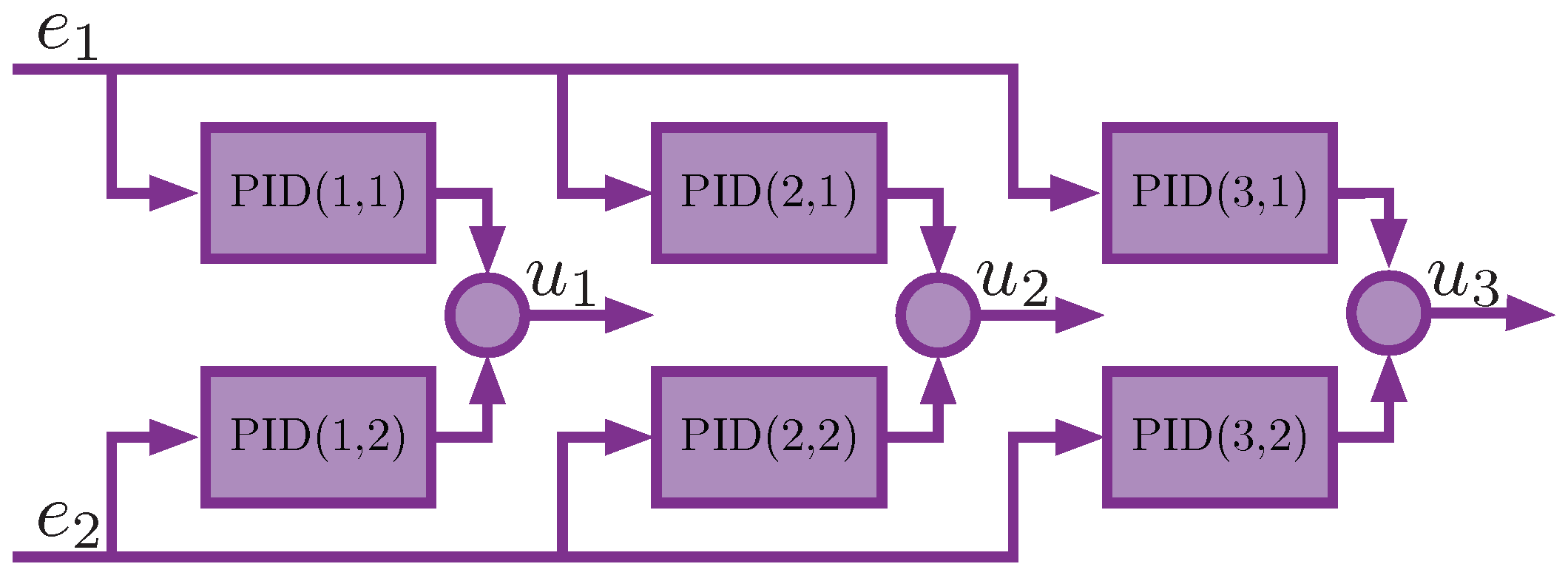
The MIMO PID controller with q inputs and m outputs consists of $q·m$ SISO PID controllers connected in a cross-coupled manner such that the q-th input is fed into each q-th SISO PID controller, and all m-th outputs are summed. An example of a MIMO PID controller with $q=2$ and $m=3$ is shown in Figure 1. The primary motivation for the utilization of MIMO PID controllers lies in the necessity to simultaneously control multiple outputs of a MIMO plant with well-coupled loops.

The interest in tuning MIMO PID controllers has been long-standing. It appears that the earliest algorithms for MIMO PID tuning can be traced back to [7,8]. Practically applicable tuning algorithms emerged with the active adoption of the LMI method in control theory [9]. It seems that the pioneering work was [10], where the synthesis of MIMO PID was formulated as a static output-feedback (SOF) synthesis problem. This idea was further developed in subsequent works [11], including the discrete-time MIMO PID synthesis method [12], although direct loop shaping was not explicitly performed in this work. Moreover, these algorithms involve less optimal practices, such as the random generation of a set of initial matrices for MIMO PID.

Another approach to synthesizing discrete MIMO PID controllers was proposed in [13], using the non-monotonic Lyapunov–Krasovskii theorem via LMIs. While this approach is intriguing, it does not allow for synthesis in the frequency domain, and the performance criteria of the system are defined in terms of weighting matrices. The issues of the robust stability of the synthesized system were not investigated.

The concept of loop shaping traces back to [14,15]. Its essence lies in defining performance requirements and robust stability margins of the closed-loop control system in terms of requirements on the singular values of the open-loop transfer function. The use of loop shaping in controller synthesis allows for direct manipulation of the frequency characteristics of the system, facilitating a trade-off between performance and robust stability margins [14]. Loop shaping gained popularity, particularly after the work in [16]. One of the early works employing loop shaping in the synthesis of MIMO PID controllers was the study in [17]. In this work, akin to classical loop shaping, a coprime factorization was used, and shaping functions were defined in the form of a pre-compensator and a post-compensator. The work in [11] is interesting in that it utilized a weighted sensitivity design.

As mentioned earlier, our approach is based on the concepts outlined in [1], which built upon the concepts introduced in [18]. The latter utilized a convex-concave procedure for tuning continuous SISO PID controllers in the frequency domain. The core principle of this method revolves around constraining the ${\mathcal{H}}_{\infty }$-norm of the closed-loop transfer functions by bounding their maximum gains across a finite yet sufficiently extensive set of frequencies. We apply the same principle but for the synthesis of a discrete MIMO PID controller. Moreover, we perform loop shaping by directly specifying the shape functions without any pre-compensators or post-compensators. The synthesis of a MIMO PID controller on an LTV plant model is rarely addressed, but its possibility was mentioned in [1]. Our study is possibly the first to adopt such an approach.

1.3. The Necessity of Employing Digital Control

When it comes to the practical implementation of control systems, the choice of the device on which the controller will be implemented is a crucial question. Analog devices were the first historically, and for SISO control systems, this option is quite suitable. An analog SISO PID controller can be implemented using three operational amplifiers.

However, for the MIMO PID controller, significantly more operational amplifiers are required. For example, to implement a MIMO PID with $q=2$ inputs and $m=3$ outputs, one would need 21 operational amplifiers (18 to implement all its components and another 3 for summing the outputs $3·q·m+q$; see Figure 1). Adding one more control loop ($q=3$, $m=4$) would increase the number of operational amplifiers to 40. The practical realization of such a device, encompassing calibration, parameter fine-tuning, or future modifications, presents formidable challenges. Furthermore, considerations must extend to the finite bandwidths and restricted signal ranges inherent in operational amplifiers. Consequently, anticipating dependable and uninterrupted functionality from such a system is, to say the least, an ambitious proposition and, in some cases, entirely impossible. Implementing the MIMO PID controller as a digital device can avoid many of these problems.

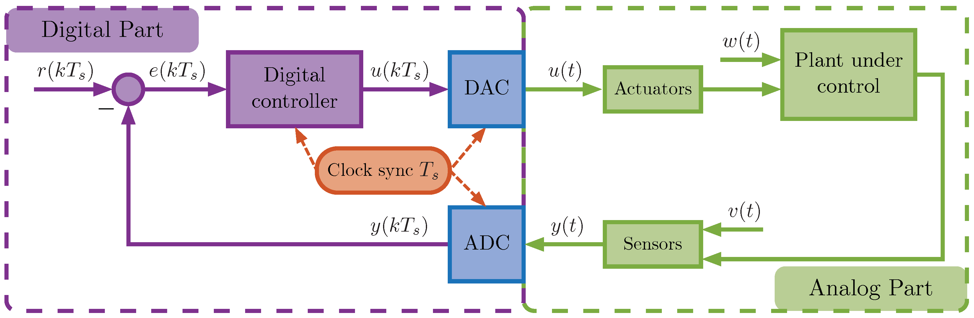
A basic digital control system (see also Figure 1.1 in [19]) is depicted in Figure 2.

The digital control system consists of two parts. In the analog part, there is a plant, which can be affected by external input disturbances $w\left(t\right)$, actuators receiving control signals $u\left(t\right)$, and sensors measuring the outputs of the plant $y\left(t\right)$, which can also be influenced by external output disturbances $v\left(t\right)$. In the digital part, there is a digital (discrete) controller, which, based on the input error vector $e\left(k{T}_s\right)$, computes the vector of control signals $u\left(k{T}_s\right)$. Additionally, there is a block that forms the reference vector $r\left(k{T}_s\right)$, an arithmetic unit calculating the error vector $e\left(k{T}_s\right)=r\left(k{T}_s\right)-y\left(k{T}_s\right)$. An Analog-to-Digital Converter (ADC) transforms the analog signal $y\left(t\right)$ into a sequence of samples (digital signal) $y\left(k{T}_s\right)$, whereas a Digital-to-Analog Converter (DAC) transforms the sequence of samples $u\left(k{T}_s\right)$ back into an analog signal $u\left(t\right)$. All components in the digital part must be time-synchronized, and the receiving, processing, and transmitting of samples should occur with a consistent sample time $T_s$. The terms “discrete controller” and “digital controller” are synonyms; the former is commonly used in the context of control theory, whereas the latter is used in the context of engineering.

Usually, the entire digital component is realized as a unified device. This device can be microcontrollers of various types, FPGA modules, or general-purpose computers. When the discrete controller is only a part of a more complex control algorithm or when there are increased demands for accuracy and fault tolerance, real-time operating system (RTOS)-controlled computers are used. The latter are also commonly referred to as real-time target machines. When simulating such a digital device in the feedback loop of the control system, it is commonly referred to as HIL (Hardware-in-the-Loop).

The number of channels in the ADC and DAC in the digital device should correspond to the number of inputs and outputs of the discrete controller. The role of the DAC in the digital system can also be performed by actuators. For example, if the actuators are voltage inverters operating in PWM mode, the signal from the digital output of the device can be directly applied to the gates of the inverter transistors.

1.4. The Necessity of Discrete Controller Synthesis

There are two approaches to obtaining the parameters for a discrete controller:

• Initially synthesize a continuous (analog) controller using the continuous-time plant model and then discretize the controller. This is currently the predominant approach.
• Initially discretize the plant model and then synthesize a discrete controller using the discrete-time plant model. This is what we use in this paper.

The discretization algorithm for both the controller and the plant model should match the type of ADCs and DACs used, typically being ZOH (Zero-Order Hold), and occasionally FOH (First-Order Hold).

The main challenge here is fundamental. According to the Kotelnikov theorem, proposed by Vladimir A. Kotelnikov in 1933 [20], also known as the Whittaker–Kotelnikov–Shannon sampling theorem or Nyquist–Shannon sampling theorem, any analog signal $y\left(t\right)$ consisting of frequencies from 0 to $f_{nyq}$ can be accurately transmitted and reconstructed using the sequence of samples $y\left(k{T}_s\right)$ taken consecutively at a rate of at least $f_s=2f_{nyq}$. Here, $f_{nyq}$ is the Nyquist frequency, $f_s=1/T_s$ is the sampling frequency (sample rate), and $T_s$ is the sample time. In digital devices, the upper bandwidth limit is critically determined by the Nyquist frequency of its ADC and DAC, a departure from analog devices where one must account for the bandwidths of individual components in the analog circuit.

The fundamental issue with the first approach lies in the fact that when synthesizing an analog controller, the effects associated with its subsequent discretization are not directly taken into consideration (see Sections 3.2 and 10 in [19]). However, for the proper operation of a digital control system, it is critically imperative to adhere to the conditions outlined in the Kotelnikov theorem. This issue is typically mitigated by introducing anti-aliasing filters in the feedback loop. Additionally, when loop shaping is employed during controller synthesis, a bandwidth is selected with a margin within the range from 0 to $f_{nyq}$ (see Section 13.3 in [3]). In cases where achieving a large margin is impractical, high-sample-rate ADCs and DACs are deployed (see Section 11 in [19]). However, it is crucial to note that an increase in the sample rate in ADCs and DACs comes with an augmented cost. Presently, there exists a significant cost discrepancy between devices with sampling frequencies of 1 kHz and 1 MHz.

In a broader context, the problem of maintaining acceptable control performance and robust stability margins during controller discretization has been extensively researched. Obviously, most of these studies focus on SISO systems (see Chapter 8 in [21]), and in the context of MIMO systems, the issues are more intricate [22]. In any case, the reality persists that the performance and robust stability margins of the discretized system are inferior to their pre-discretization counterparts, and the extent of this degradation is contingent on the sample time–larger sample times result in diminished performance and robust stability margins. The closer the crossover frequencies of the control system are to the Nyquist frequency, the more the robust stability margin degrades in the discretized control system (see Section 5.2 in [19]). This becomes more apparent when regarding continuous systems as a specific case of discrete systems when $T_s\to 0$.

In summary, opting for the first approach will yield a control system significantly different from the one obtained when synthesizing the controller in continuous time. It is a well-known fact that the frequency responses of the discretized system and the original continuous system will closely match only at low frequencies.

In the second approach, all discretization effects are inherently captured in the discrete-time model of the plant on which the discrete controller is synthesized. The synthesized digital control system possesses precisely the performance and robust stability margins specified during the discrete controller synthesis. This extends to the frequency responses of the digital system as well. By applying loop shaping, we can directly shape the frequency responses of the digital control system. For instance, achieving a certain robust stability margin in the closed-loop system may eliminate the need for using anti-aliasing filters in the feedback loop of the digital control system. All of this serves as the primary motivation for the direct synthesis of a discrete controller.

2. Terminology and Notations

The following symbols/notations are used in this paper:

• $A⪰0$ denotes that the Hermitian matrix A is positive semi-definite: $x^{\mathrm{H}}Ax\ge 0,\forall x,A=A^{\mathrm{H}},x\in {\mathbb{C}}^n,A\in {\mathbb{C}}^{n\times n}$;
• $x\ge y$ denotes that the scalar x is greater than or equal to the scalar y;
• $A⪯0$ denotes that the Hermitian matrix A is negative semi-definite: $x^{\mathrm{H}}Ax\le 0,\forall x,A=A^{\mathrm{H}},x\in {\mathbb{C}}^n,A\in {\mathbb{C}}^{n\times n}$;
• $x\le y$ denotes that the scalar x is less than or equal to the scalar y;
• $A⪰B$ denotes that the matrix $A-B$ is positive semi-definite: $A-B⪰0$;
• $A^{\mathrm{H}}$ denotes the (Hermitian) conjugate transpose of the matrix A;
• ${\parallel A\parallel }_2=\overline{\sigma }\left(A\right)$ denotes the spectral norm of the matrix A;
• $\overline{\sigma }\left(A\right)$ denotes the maximum singular value of the matrix A;
• $\underline{\sigma }\left(A\right)$ denotes the minimum singular value of the matrix A;
• ${\parallel G\left(z\right)\parallel }_{\infty }$ denotes the ${\mathcal{H}}_{\infty }$-norm of the matrix function $G\left(z\right)$;
• $A^{†}$ denotes the Moore–Penrose inverse of the matrix $A\in {\mathbb{C}}^{q\times m}$:
  if the matrix $A{A}^{\mathrm{H}}\in {\mathbb{C}}^{q\times q}$ is invertible, then $A^{†}=A^{\mathrm{H}}{\left(A{A}^{\mathrm{H}}\right)}^{-1},A{A}^{†}=I_q$;
  if the matrix $A^{\mathrm{H}}A\in {\mathbb{C}}^{m\times m}$ is invertible, then $A^{†}={\left(A^{\mathrm{H}}A\right)}^{-1}{A}^{\mathrm{H}},A^{†}A=I_m$;
• $A^{-1}$ denotes the inverse of the square matrix $A\in {\mathbb{C}}^{n\times n}$:
  if the matrix A is invertible (nonsingular), then $A{A}^{-1}=A^{-1}A=I_n$;
• $I_n$ denotes the $n\times n$ identity matrix, $I_n\in {\mathbb{R}}^{n\times n}$;
• $\exp \left(x\right)=e^x$, where e is the base of natural logarithms (the Euler number);
• $T_s$ is the sample time and $f_s=1/T_s$ is the sampling frequency;
• $\omega =2\pi f$ is the angular frequency.

The singular values of a matrix $A\in {\mathbb{C}}^{m\times n}$ are the non-negative square roots of the eigenvalues of $A{A}^{\mathrm{H}}$ [23]

$${\sigma }_i\left(A\right)=+\sqrt{{\lambda }_i\left(A{A}^{\mathrm{H}}\right)},{\sigma }_i\left(A\right)\in {\mathbb{R}}^1,$$

arranged in non-increasing order:

$${\sigma }_1\left(A\right)\ge {\sigma }_2\left(A\right)\ge \cdots \ge {\sigma }_n\left(A\right)\ge 0,\overline{\sigma }\left(A\right)={\sigma }_1\left(A\right),\underline{\sigma }\left(A\right)={\sigma }_n\left(A\right).$$

If the matrix A is invertible, then

$$\underline{\sigma }\left(A\right)=1/\overline{\sigma }\left(A^{-1}\right),\overline{\sigma }\left(A\right)=1/\underline{\sigma }\left(A^{-1}\right).$$

The condition number $\kappa \left(A\right)$ is defined as the ratio of the maximum and minimum singular values of the matrix A:

$$\kappa \left(A\right)=\frac{\overline{\sigma }\left(A\right)}{\underline{\sigma }\left(A\right)}.$$

The invertible matrix $A\in {\mathbb{C}}^{n\times n}$ is a unitary matrix if

$$A^{\mathrm{H}}A=A{A}^{\mathrm{H}}=A{A}^{-1}=I_n,\mathrm{then}\kappa \left(A\right)=1,{\sigma }_1\left(A\right)=\cdots ={\sigma }_n\left(A\right)=1.$$

2.1. Some Important Aspects of Control Theory

The Z-transform, first proposed in [24], is obtained from the discrete Laplace transform, first proposed in [25], by substituting

$$\begin{array}{c}\hfill exp\left(s{T}_s\right)⟶z,\sum _{n=0}^{\infty }x\left[n\right]exp(-s{T}_{s}n)⟶\sum _{n=0}^{\infty }x\left[n\right]z^{-n},\end{array}$$

where s is the Laplace transform variable and z is the Z-transform variable.

The discrete MIMO transfer function $G\left(z\right)\in {\mathbb{C}}^{q\times m}$ is a matrix function that relates the Z-transforms of the inputs vector $u\left(z\right)\in {\mathbb{C}}^m$ and the outputs vector $y\left(z\right)\in {\mathbb{C}}^q$ for the system with zero initial conditions: $y\left(z\right)=G\left(z\right)u\left(z\right)$.

The discrete-time MIMO frequency response is the complex matrix function that is represented by

$$G\left(exp\left(j\omega T_s\right)\right)\in {\mathbb{C}}^{q\times m},$$

and it is obtained by applying the discrete-time Fourier transform to the impulse response of $G\left(z\right)$. To obtain the value of the discrete-time MIMO frequency response at frequency $\omega$, we need to substitute $z⟶exp\left(j\omega T_s\right)$ in the discrete-time MIMO transfer function $G\left(z\right)$. This substitution follows from the definitions of the Z-transform and the discrete Fourier transform, as shown below:

$$\begin{array}{c}\hfill z⟶exp\left(j\omega T_s\right),\sum _{n=0}^{\infty }x\left[n\right]z^{-n}⟶\sum _{n=0}^{\infty }x\left[n\right]exp(-j\omega T_{s}n).\end{array}$$

The details of this substitution are presented in Chapter 8 in [26].

The maximum gain of the discrete MIMO transfer function $G\left(z\right)$ at the frequency $\omega$, denoted as $\parallel G\left(exp\left(j\omega T_s\right)\right){\parallel }_2$, is the spectral norm (maximum singular value) of the matrix, which represents the value of the discrete-time MIMO frequency response at the frequency $\omega$

$$\parallel G\left(exp\left(j\omega T_s\right)\right){\parallel }_2=\overline{\sigma }\left(G\left(exp\left(j\omega T_s\right)\right)\right)\in {\mathbb{R}}^1,$$

whereas the minimum gain of the discrete MIMO transfer function at the frequency $\omega$ is the minimum singular value of this frequency response.

The ${\mathcal{H}}_{\infty }$-norm of the discrete MIMO transfer function $G\left(z\right)$, denoted as ${\parallel G\left(z\right)\parallel }_{\infty }$, is the frequency peak that yields the maximum gain of the discrete MIMO transfer function over all frequencies $\omega \in [0,\dots ,{\omega }_{nyq}]$

$$\parallel G\left(z\right){\parallel }_{\infty }=\underset{\omega }{sup}\left\{\overline{\sigma }\left(G\left(exp\left(j\omega T_s\right)\right)\right)\right\}\in {\mathbb{R}}^1.$$

The Nyquist frequency is defined as half of the sampling frequency:

$$f_{nyq}=f_s/2=1/\left(2T_s\right),{\omega }_{nyq}=2\pi f_{nyq}=\pi /T_s.$$

According to the fundamental Kotelnikov theorem [20], the maximum frequency component that can be reconstructed from a discrete signal is bounded by the Nyquist frequency. Therefore, it is important to choose an appropriate sampling frequency to accurately represent the plant model.

2.2. The Symmetry of the Discrete Fourier Transform

In the definition of the ${\mathcal{H}}_{\infty }$-norm of the discrete MIMO transfer function, it was stated that all frequencies $\omega \in [0,\dots ,{\omega }_{nyq}]$. This follows from the symmetry of the discrete Fourier transform, which we briefly demonstrate below. A more detailed proof of the symmetry of the discrete Fourier transform can be found in Section 3.2 in [27].

The discrete Fourier transform $X\left[k\right]$ of a sequence of samples (digital signal) $x\left[n\right]$ is defined by the following equation:

$$X\left[k\right]=\sum _{n=0}^{N-1}x\left[n\right]exp(-j2\pi kn/N),k=f_k{T}_s=\frac{{\omega }_k}{2\pi }{T}_s,k=0,1,\dots ,N-1,$$

where k is the frequency index and $n=0,1,\dots ,N-1$ is the time index.

Let us compute the discrete Fourier transform for a frequency that is an integer multiple of the Nyquist frequency, i.e., for $k=k_{nyq}N$:

$$k_{nyq}=\frac{{\omega }_{nyq}}{2\pi }{T}_s=\frac{1}{2},k_{nyq}N=\frac{N}{2},$$

$$X\left[k_{nyq}N\right]=\sum _{n=0}^{N-1}x\left[n\right]exp(-j2\pi k_{nyq}Nn/N)=\sum _{n=0}^{N-1}x\left[n\right]exp{(-j\pi )}^n.$$

Using the Euler identity $exp\left(j\pi \right)=exp(-j\pi )=-1$, we obtain

$$X\left[k_{nyq}N\right]=\sum _{n=0}^{N-1}x\left[n\right]{(-1)}^n.$$

This means that when computing $X\left[k\right]$, the frequency component $X\left[k_{nyq}N\right]$ will serve as a factor that ensures complex conjugation. That is, when we consider frequencies above the Nyquist frequency, we do not obtain any additional information since those frequency components are mirrored and can be represented by those below the Nyquist frequency. Therefore, it is sufficient to consider frequencies in the range $[0,\dots ,{\omega }_{nyq}]$ when computing the ${\mathcal{H}}_{\infty }$-norm of the discrete MIMO transfer function.

When we perform the synthesis of the discrete MIMO PID controller on the frequency range $[0,\dots ,{\omega }_{nyq}]$, we can say that “we are synthesizing a MIMO PID controller across the entire frequency range”. Note that this cannot be said in the case of continuous-time MIMO PID synthesis, as described in [1], because then the synthesis will need to be performed on an infinite frequency range $[0,\dots ,\infty ]$ (in practice, $[0,\dots ,{\omega }_n]$, where ${\omega }_n$ is a sufficiently large frequency).

2.3. The Small-Gain Theorem

The small-gain theorem, initially proposed in [28], is a simple and intuitively understandable tool for computing robust stability margins in terms of ${\mathcal{H}}_{\infty }$-norms. To apply this theorem in robust analysis, the so-called $M-\Delta$ configuration (see Chapter 7 in [29] and Section 8.2 in [30]) is utilized, where the control system with uncertainties is divided into a nominal (unperturbed) part, represented by the transfer function $M\left(z\right)$, and a part with uncertainties (perturbed), represented by the transfer function $\Delta \left(z\right)$. Such a control system will be stable if and only if (see Section 10.4 in [31]):

$$\parallel M\left(z\right){\parallel }_{\infty }·\parallel \Delta \left(z\right){\parallel }_{\infty }<1.$$

We consider only two cases of uncertainties, which are sufficient for our goal (and in most practical cases), where only the plant model has output multiplicative uncertainty (Figure 3) and output additive uncertainty (Figure 4). The controller is assumed to be precisely known without uncertainties.

In the case of output multiplicative (OM) uncertainty, the transfer functions $M_{OM}\left(z\right)$ and ${\Delta }_{OM}\left(z\right)$ relate the vectors v and y as follows: $v={\Delta }_{OM}\left(z\right)y$, $y=M_{OM}\left(z\right)v$, and the transfer function $M_{OM}\left(z\right)$ takes the form

$$M_{OM}\left(z\right)=-P\left(z\right)C\left(z\right){\left(I+P\left(z\right)C\left(z\right)\right)}^{-1}=-{\left(I+P\left(z\right)C\left(z\right)\right)}^{-1}P\left(z\right)C\left(z\right).$$

(1)

Refer to Appendix A for the proof of this identity.

In the case of output additive (OA) uncertainty, the transfer functions $M_{OA}\left(z\right)$ and ${\Delta }_{OA}\left(z\right)$ relate the vectors v and u as follows: $v={\Delta }_{OA}\left(z\right)u$, $u=M_{OA}\left(z\right)v$, and the transfer function $M\left(z\right)$ takes the form

$$M_{OA}\left(z\right)=-C\left(z\right){\left(I+P\left(z\right)C\left(z\right)\right)}^{-1}.$$

(2)

Thus, if the ${\mathcal{H}}_{\infty }$-norm of $M\left(z\right)$ in the control system is bounded, the value $1/{\parallel M\left(z\right)\parallel }_{\infty }$ will determine the margin of robust stability for the closed-loop system with uncertainties. This is because it serves as the bound for the ${\mathcal{H}}_{\infty }$-norm of $\Delta \left(z\right)$, representing the maximum gain of the possible feedback perturbations in the closed-loop system:

$${\parallel \Delta \left(z\right)\parallel }_{\infty }<\frac{1}{{\parallel M\left(z\right)\parallel }_{\infty }}.$$

3. The Statement of the Problem

We aim to design the stationary discrete MIMO PID controller for the discrete linear non-stationary plant model. In this context, we have the LTI controller, while the plant will be described by an LTV model. Below, we demonstrate our approximation of the LTV plant model through an array of LTI models.

Through this design approach, we guarantee the robust stability margin and performance for all linear plant models included in the array. The proposed synthesis of the MIMO PID controller will be achieved by solving a system of LMIs. If a numerical solution exists for these LMIs, the performance and stability of the closed-loop system with the non-stationary plant model are guaranteed, even in the worst-case scenario.

3.1. The Plant Model

The MIMO LTV plant model is generally represented as a linear continuous-time model in the state-space form:

$$\begin{array}{c}\left\{\begin{array}{c}\dot{x}\left(t\right)=A\left(t\right)x\left(t\right)+B\left(t\right)u\left(t\right),\hfill \\ y\left(t\right)=C\left(t\right)x\left(t\right)+D\left(t\right)u\left(t\right),\hfill \end{array}\right.\end{array}$$

(3)

where $y\left(t\right)\in {\mathbb{R}}^q$, $u\left(t\right)\in {\mathbb{R}}^m$, $x\left(t\right)\in {\mathbb{R}}^s$; q represents the number of outputs; m is the number of inputs; and s is the number of states (model order). The state-space matrices $A\left(t\right)$, $B\left(t\right)$, $C\left(t\right)$, and $D\left(t\right)$ vary in time. We consider two of the most practically relevant cases, in our view, that allow representing the LTV model as an array of LTI models.

3.1.1. The LPV Model

The first case is the linear parameter-varying (LPV) model

$$\left\{\begin{array}{c}\dot{x}\left(t\right)=A\left(\theta \left(t\right)\right)x\left(t\right)+B\left(\theta \left(t\right)\right)u\left(t\right),\hfill \\ y\left(t\right)=C\left(\theta \left(t\right)\right)x\left(t\right)+D\left(\theta \left(t\right)\right)u\left(t\right),\hfill \end{array}\right.$$

(4)

where $\theta \left(t\right)$ is the function of time-varying plant parameters [32]. Here, it is important that the function $\theta \left(t\right)$ is deterministic, and therefore, the varying state-space matrices are deterministic (see Section 1.2 in [33]). Most often, an LPV model is obtained by linearizing a nonlinear model at several time points. It can also be derived through system identification methods [34] or when the state-space matrices contain parameters with variations explicitly defined over time.

In this case, we use the index n to denote the time point $t_n$ at which the LTI model was calculated, obtaining an array of state-space matrices:

$${\theta }_n=\theta \left(t_n\right),\left\{A_n=A\left({\theta }_n\right),B_n=B\left({\theta }_n\right),C_n=C\left({\theta }_n\right),D_n=D\left({\theta }_n\right)\right\}.$$

The conditions described at the beginning of Section 3 (guaranteeing performance and robustness) will be satisfied if the interval for calculating the LTI models is equal to the sample time during its discretization. If this is challenging, our problem formulation requires $\theta \left(t\right)$ to be a linear function, leading to linear interpolation of parameters between time points $t_n$ during modeling. In any case, it is essential to consider how well the LPV model with linear interpolation of parameters will describe the dynamics of a real plant. Moreover, the grid on which the interpolation of the array of LTI models will be performed may be irregular.

3.1.2. The Uncertain State-Space Model

The second case is the uncertain state-space model

$$\left\{\begin{array}{c}\dot{x}\left(t\right)=A\left(\delta \left(t\right)\right)x\left(t\right)+B\left(\delta \left(t\right)\right)u\left(t\right),\hfill \\ y\left(t\right)=C\left(\delta \left(t\right)\right)x\left(t\right)+D\left(\delta \left(t\right)\right)u\left(t\right),\hfill \end{array}\right.$$

(5)

where $\delta \left(t\right)$ is the function that represents the uncertain plant parameters. Here, it is important that the function $\delta \left(t\right)$ is non-deterministic, but the bounds of the interval in which it can vary must be known. All state-space matrices of such a system must be representable in the following form:

$$A\left(\delta \left(t\right)\right)=A_0+A_{\Delta }\left(\delta \left(t\right)\right),A_{\Delta }\left(\delta \left(t\right)\right)={\delta }_1\left(t\right)A_1+{\delta }_2\left(t\right)A_2+\cdots +{\delta }_{N_i}\left(t\right)A_{N_i}$$

where $A_0$ is the nominal part and $A_{\Delta }\left(\delta \left(t\right)\right)$ is the perturbed part that can vary randomly within the bounds specified by $\delta \left(t\right)$ (see Section 4.3.1 in [35]).

Such a representation of the plant model is typical for situations where its parameters have measurement uncertainties. In this case, the perturbation parameters form a set represented by a regular polyhedron:

$${\Delta }_I=\left\{\delta \left(t\right)|{\delta }_i\left(t\right)\in [{\delta }_i^{-},{\delta }_i^{+}],i=1,\dots ,N_i\right\},$$

with a set of extreme points: ${\Delta }_E=\left\{{\delta }_i|{\delta }_i={\delta }_i^{-}\mathrm{or}{\delta }_i^{+},i=1,\dots ,N_i\right\}.$

If the perturbation parameters are normalized, they form a polytope:

$${\Delta }_P=\left\{\delta \left(t\right)|\sum _{i=1}^{N_i}{\delta }_i\left(t\right)=1,{\delta }_i\left(t\right)\ge 0\right\},$$

with a set of extreme points ${\Delta }_E=\left\{e_i^{\mathrm{T}}|e_i\in {\mathbb{R}}^{N_i},i=1,\dots ,N_i\right\},$ where $e_i$ is the basis vector, with each i-th element equal to 1, while all the others are zero. The details of these representations are described in Section 4.3 in [35].

According to Theorem 4.3 in [35], to guarantee the performance and robustness of the closed-loop system, similar to what was proposed for the LPV model, it is sufficient to synthesize the controller on an array of LTI models calculated at the extreme points of the perturbation parameters set.

In this case, we use the index n to denote the extreme points ${\delta }_n$ of the perturbation parameters set at which the LTI model was calculated, obtaining an array of state-space matrices:

$${\delta }_n\in {\Delta }_E,\left\{A_n=A\left({\delta }_n\right),B_n=B\left({\delta }_n\right),C_n=C\left({\delta }_n\right),D_n=D\left({\delta }_n\right)\right\}.$$

3.1.3. The Array of Discrete Transfer Functions

Both of the described cases result in approximating the LTV plant model as an array of LTI models with an index n for the synthesis of a robust discrete controller:

$$\left\{\begin{array}{c}{\dot{x}}_n\left(t\right)=A_n{x}_n\left(t\right)+B_n{u}_n\left(t\right),\hfill \\ y_n\left(t\right)=C_n{x}_n\left(t\right)+D_n{u}_n\left(t\right),\hfill \end{array}\right.$$

where $x_n\left(t\right)$, $u_n\left(t\right)$, and $y_n\left(t\right)$ are the state, input, and output vectors of the n-th LTI plant model, respectively. These cases can also be combined. In fact, by combining them, it is possible to represent any LTV model as an array of LTI models.

After that, it is necessary to discretize each LTI model in the array using the ZOH or FOH method, depending on the type of ADC and DAC used in the digital control system. When using the ZOH method (see Section 4.3.3 in [19]), we obtain

$$t\left(T_{s}k\right)\le t\le t(T_{s}k+T_s),k\in \mathbb{Z},$$

$$A_n^d=exp\left(A_n{T}_s\right),B_n^d=A_n^{-1}(A_n^d-I_s)B_n,C_n^d=C_n,D_n^d=D_n.$$

Here, the index k denotes the sample index. Thus, we obtain an array of LTI discrete-time state-space plant models:

$$\left\{\begin{array}{c}{x}_n(T_{s}k+T_s)=A_n^{d}x\left(T_{s}k\right)+B_n^d{u}_n\left(T_{s}k\right),\hfill \\ y_n\left(T_{s}k\right)=C_n^d{x}_n\left(T_{s}k\right)+D_n^d{u}_n\left(T_{s}k\right).\hfill \end{array}\right.$$

As our method operates with transfer functions, we also derive an array of discrete transfer functions:

$$P_n\left(z\right)=C_n^d{(z{I}_s-A_n^d)}^{-1}{B}_n^d+D_n^d,P_n\left(z\right)\in {\mathbb{C}}^{q\times m},n\in \mathbb{N}.$$

(6)

3.2. The Transfer Function of the Controller

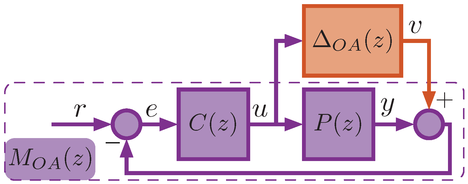
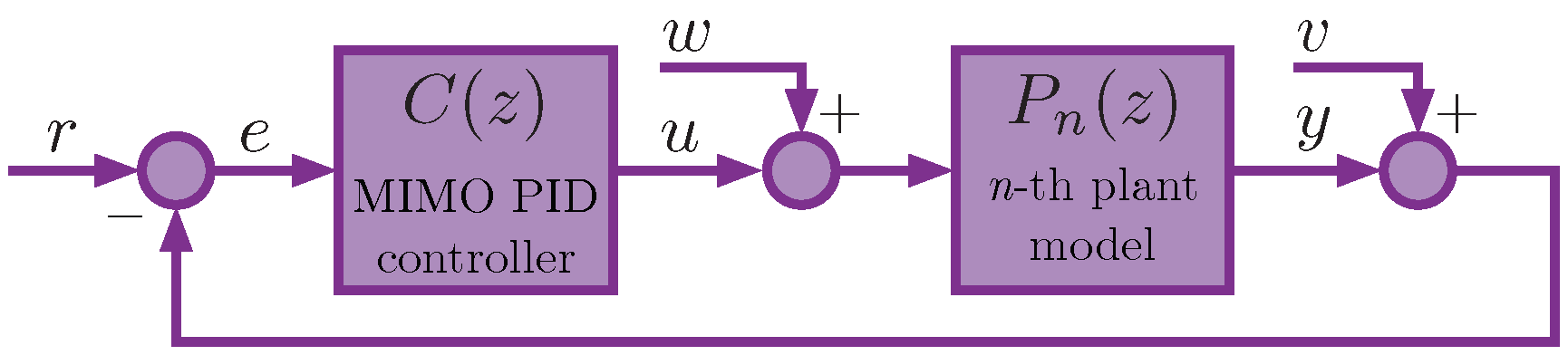
We employ the feedback connection scheme depicted in Figure 5, which is the classic scheme commonly used in tracking control systems. The scheme is based on the utilization of the MIMO PID controller, which provides feedback control to the output of the plant model.

Here, the vector r is the reference vector, the vector e denotes the error signal, the vector u is the plant control input, and the vector y is the plant output. Additionally, the vector w represents the input disturbance vector and the vector v represents the output disturbance vector.

The discrete LTI model of the MIMO PID controller in the control law

$$u\left(z\right)=C\left(z\right)e\left(z\right),u\left(z\right)\in {\mathbb{C}}^m,e\left(z\right)\in {\mathbb{C}}^q$$

is defined as a discrete transfer function in the form:

$$C\left(z\right)=K_P+K_I\frac{z{T}_s}{z-1}+K_D\frac{z-1}{z{T}_s},C\left(z\right)\in {\mathbb{C}}^{m\times q},$$

(7)

where the MIMO PID controller coefficients $\left\{K_P,K_I,K_D\right\}\in {\mathbb{R}}^{m\times q}$ are arbitrary (non-diagonal) matrices. An evident requirement for MIMO tracking control systems is that the number of inputs (m) and outputs (q) of the plant should satisfy

$$m\ge q.$$

Here, we use the backward Euler numerical method

$$\frac{z{T}_s}{z-1}$$

for both discrete differentiation and integration. We can use another method for integration and differentiation, such as

$$\begin{array}{cc}\hfill \mathrm{Forward}\mathrm{Euler}:& \frac{T_s}{z-1},\hfill \\ \hfill \mathrm{or}\mathrm{Tustin}\left(\mathrm{Trapezoidal}\right):& \frac{T_s}{2}·\frac{z+1}{z-1}.\hfill \end{array}$$

Details of these methods can be found in Section 6.1 in [19]. However, it is advisable to avoid using the forward Euler method in the differentiator since it would require introducing a derivative-filter time constant. This constant cannot be a tunable parameter in our problem formulation due to nonlinearity, and it would need to be manually specified as a scalar or matrix in case different derivative filter time constants are required in each control loop. The use of the backward Euler method in the differentiator, apart from not requiring the use of a derivative-filter time constant, also allows for implementing finite control in the differentiator, as it sets some of the closed-loop poles to zero $z=0$. This is somewhat analogous to “deadbeat control” where all closed-loop poles are set to zero. In the continuous system, this is equivalent to the unrealizable case when the pole $s=-\infty$.

Moreover, we can add or remove components of the MIMO PID controller; for example, we can remove components $K_P$ and $K_D$ when not needed, turning the “PID” controller into “PI”, “ID”, or “I”. We can add integrator or differentiator components of the second order and higher. Our problem formulation explicitly requires the presence of an integrator, which is natural since without it, minimizing the error vector in the steady state in a MIMO system would be impossible.

3.3. The Array of Discrete Transfer Functions

In accordance with the diagram in Figure 5, we define the following array of discrete transfer functions:

• The open-loop transfer function $L\left(z\right)$, which is a transfer function from the error vector e to the output vector y

  $$y\left(z\right)=L_n\left(z\right)e\left(z\right),L_n\left(z\right)=P_n\left(z\right)C\left(z\right),y\left(z\right)\in {\mathbb{C}}^q,L_n\left(z\right)\in {\mathbb{C}}^{q\times q},$$

  where $P_n\left(z\right)$ represents the n-th plant model from the array of linear plant models (6).
• The sensitivity function $S\left(z\right)$, which is a closed-loop transfer function from the reference vector r to the error vector e

  $$e\left(z\right)=S_n\left(z\right)r\left(z\right),S_n\left(z\right)={\left(I_q+L_n\left(z\right)\right)}^{-1},S_n\left(z\right)\in {\mathbb{C}}^{q\times q}.$$
• The complementary sensitivity function $T\left(z\right)$, which is a closed-loop transfer function from the reference vector r to the output vector y

  $$y\left(z\right)=T_n\left(z\right)r\left(z\right),T_n\left(z\right)=I_q-S_n\left(z\right)=L_n\left(z\right)S_n\left(z\right),T_n\left(z\right)\in {\mathbb{C}}^{q\times q}.$$
• The static and low-frequency sensitivity function $F\left(z\right)$, which is the sensitivity function for small frequencies. If $C\left(z\right)$ is given by (7), it takes the form:

  $$F_n\left(z\right)={\left(P_n\left(1\right)K_I{T}_s\right)}^{-1}(z-1),F_n\left(z\right)\approx S_n\left(z\right)\mathrm{for}\mathrm{small}\omega ,z=exp\left(j\omega T_s\right),$$

  (8)

  where $P_n\left(1\right)$ is the static gain of the n-th plant model, which means the frequency response at zero frequency ($\omega =0$). See Appendix B for a detailed explanation of the static and low-frequency sensitivity function.
• The Q-parameter (a term from the Youla parametrization approach [36]), is a closed-loop transfer function from the reference vector r to the input vector u

  $$u\left(z\right)=Q_n\left(z\right)r\left(z\right),Q_n\left(z\right)=C\left(z\right)S_n\left(z\right),Q_n\left(z\right)\in {\mathbb{C}}^{m\times q}.$$
• The closed-loop transfer function from the input disturbance vector w to the error vector e is:

  $$e\left(z\right)=W_n\left(z\right)w\left(z\right),W_n\left(z\right)=-S_n\left(z\right)P_n\left(z\right),w\left(z\right)\in {\mathbb{C}}^m,W_n\left(z\right)\in {\mathbb{C}}^{q\times m}.$$
• The closed-loop transfer function from the output disturbance vector v to the error vector e is:

  $$e\left(z\right)=V_n\left(z\right)v\left(z\right),V_n\left(z\right)=-S_n\left(z\right),v\left(z\right)\in {\mathbb{C}}^q,V_n\left(z\right)\in {\mathbb{C}}^{q\times q}.$$

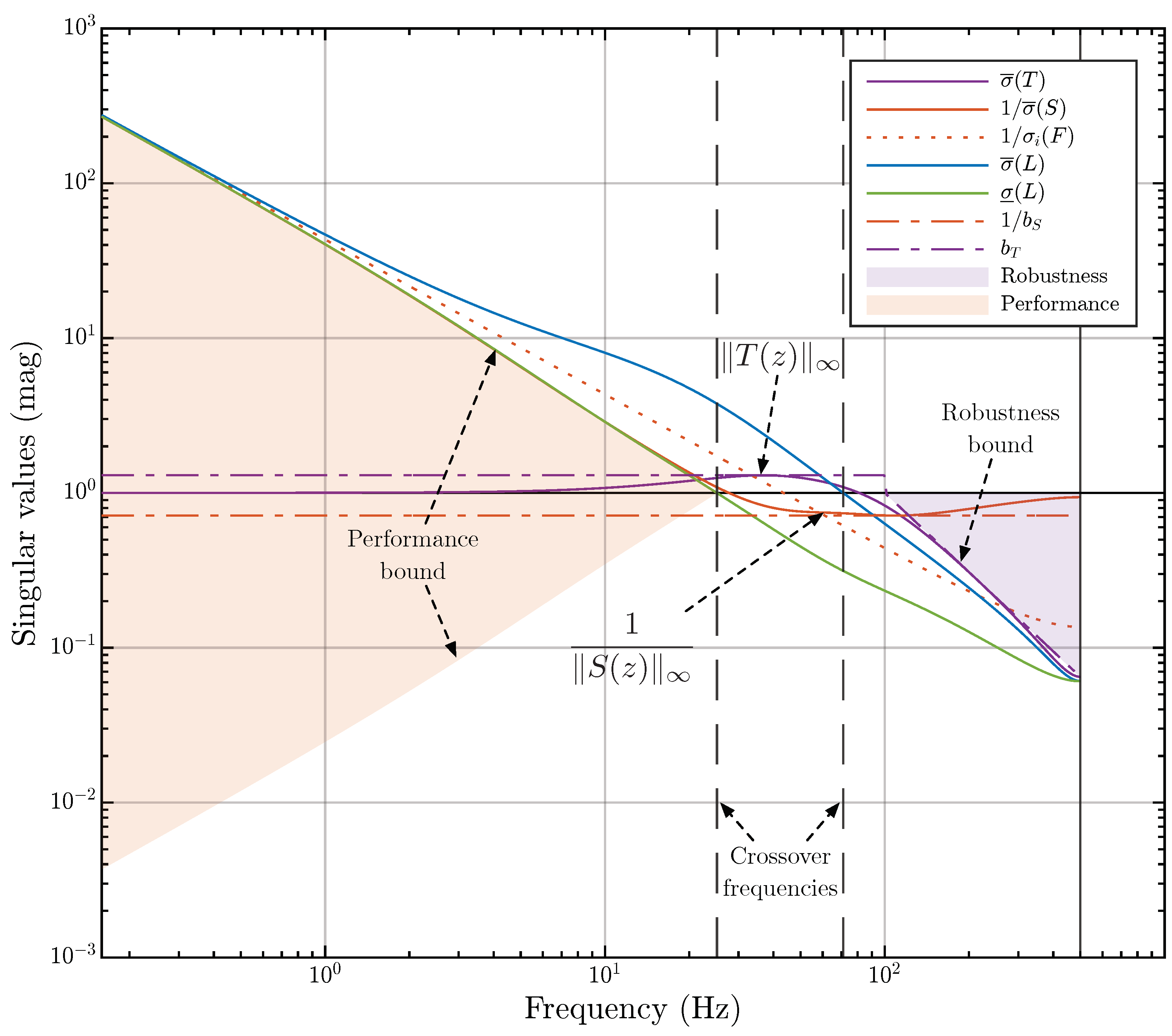
3.4. The Performance Criteria

Using these closed-loop transfer functions, we formulate the performance criteria [31] of the closed-loop control system with the MIMO PID controller in terms of the ${\mathcal{H}}_{\infty }$-norm constraints on the closed-loop transfer functions.

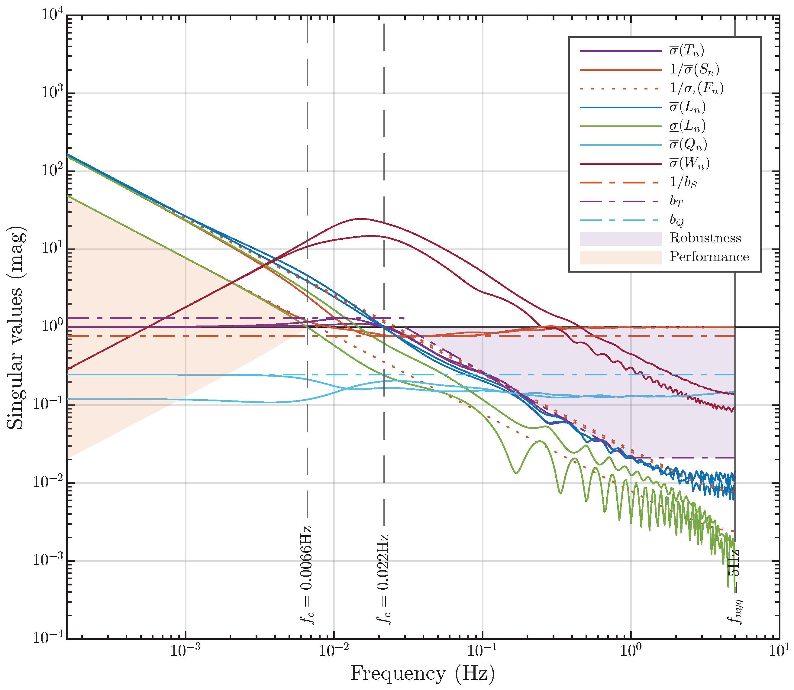
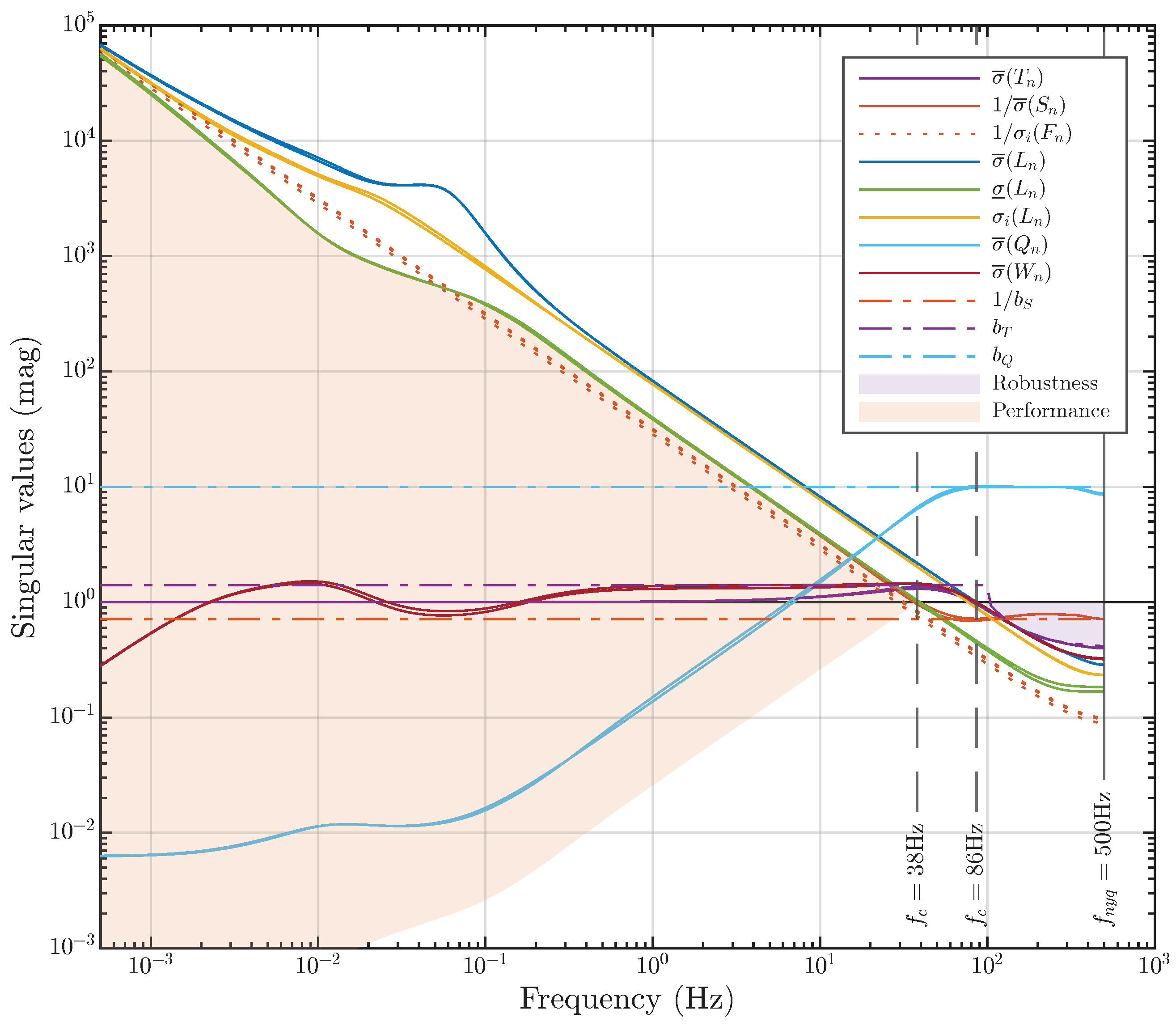
The restriction of the ${\mathcal{H}}_{\infty }$-norm of the sensitivity function $S_n\left(z\right)$ guarantees the performance of the closed-loop system for all plant models $P_n\left(z\right)$. This also determines the maximum overshoot in the closed-loop control system.

The restriction of the ${\mathcal{H}}_{\infty }$-norm of the complementary sensitivity function $T_n\left(z\right)$ guarantees the robust stability of the closed-loop system for all plant models $P_n\left(z\right)$. Additionally, according to the small-gain theorem, the value $1/{∥T\left(z\right)∥}_{\infty }$ determines the margin of robust stability for the control system in the case of output multiplicative uncertainties in the plant model (1) since

$${∥M_{OM}\left(z\right)∥}_{\infty }={∥T\left(z\right)∥}_{\infty }$$

(9)

and serves as a bound for the maximum gain of the possible output multiplicative disturbances in the plant model

$$\parallel {\Delta }_{OM}{\left(z\right)\parallel }_{\infty }<\frac{1}{{\parallel T\left(z\right)\parallel }_{\infty }}.$$

The transfer functions $S\left(z\right)$ and $T\left(z\right)$ are related by the fundamental equation

$$S\left(z\right)+T\left(z\right)=I_q.$$

In a stable closed-loop system with a small steady-state tracking error, it holds that

$${∥S(exp(0\left)\right)∥}_2={∥T(exp\left(j{\omega }_{nyq}{T}_s\right))∥}_2\approx 0,{∥S(exp\left(j{\omega }_{nyq}{T}_s\right))∥}_2={∥T(exp(0\left)\right)∥}_2\approx 1.$$

In the ideal case, ${∥S\left(z\right)∥}_{\infty }={∥T\left(z\right)∥}_{\infty }=1$, which means perfect tracking across the entire frequency range. In reality, such a restriction would be too stringent and may require excessively large input signals. Rational values for ${∥S\left(z\right)∥}_{\infty }$ and ${∥T\left(z\right)∥}_{\infty }$ typically range from 1.1 to 1.8.

By applying a constraint on the ${\mathcal{H}}_{\infty }$-norm of $Q\left(z\right)$, we limit the magnitude of the input of the plant model. This is useful in accounting for physical limitations, such as those in the actuator devices. Additionally, according to the small-gain theorem, the value $1/{∥Q\left(z\right)∥}_{\infty }$ determines the margin of robust stability for the control system in the case of output additive uncertainties in the plant model (2) since

$${∥M_{OA}\left(z\right)∥}_{\infty }={∥Q\left(z\right)∥}_{\infty }$$

(10)

and serves as a bound for the maximum gain of the possible output additive disturbances in the plant model

$$\parallel {\Delta }_{OA}{\left(z\right)\parallel }_{\infty }<\frac{1}{{\parallel Q\left(z\right)\parallel }_{\infty }}.$$

The rational values of ${∥Q\left(z\right)∥}_{\infty }$ should be multiples of $1/\underline{\sigma }\left(P\left(1\right)\right)$ (see Section 3.1 in [1]).

By constraining the ${\mathcal{H}}_{\infty }$-norms of $W\left(z\right)$ and $V\left(z\right)$, we limit the effect of the input and output disturbance vectors on the error vector. Note that there is no need to constrain the ${\mathcal{H}}_{\infty }$-norm of $V_n\left(z\right)$ because

$$\parallel V_n{\left(z\right)\parallel }_{\infty }=\parallel -S_n{\left(z\right)\parallel }_{\infty }={\parallel S_n\left(z\right)\parallel }_{\infty }.$$

We aim to achieve the lowest possible settling time for the closed-loop system while adhering to the constraints of the ${\mathcal{H}}_{\infty }$-norm of other transfer functions. We cannot constrain the ${\mathcal{H}}_{\infty }$-norm of $F\left(z\right)$ since, as defined in (8), an unbounded increase in z results in an infinite value of ${∥F\left(z\right)∥}_{\infty }$. Instead, we minimize the spectral norm of the matrix

$${\left(P_n\left(1\right)K_I{T}_s\right)}^{-1},$$

(11)

which we hereafter refer to as the matrix of the static and low-frequency sensitivity (SLFS). This will result in attaining the best possible static and low-frequency sensitivity, which requires minimizing

$$\min {∥{\left(P_n\left(1\right)K_I{T}_s\right)}^{-1}∥}_2.$$

Minimizing the spectral norm of the SLFS matrix, along with constraining the ${\mathcal{H}}_{\infty }$-norm of $S\left(z\right)$ and $T\left(z\right)$, ensures the decoupling of control loops in the closed-loop system, at least at low frequencies. This is discussed in more detail in Section 4.6.

3.5. The SDP Formulation

We can now formulate the problem of synthesizing a MIMO PID controller as the semi-definite programming (SDP) problem:

$$\left\{\begin{array}{cc}\min \hfill & \parallel {\left(P_n\left(1\right)K_I{T}_s\right)}^{-1}{\parallel }_2,\hfill \\ \mathrm{s}.\mathrm{t}.\hfill & \parallel S_n{\left(z\right)\parallel }_{\infty }\le S_{\max },\hfill \\ \hfill & \parallel T_n{\left(z\right)\parallel }_{\infty }\le T_{\max },\hfill \\ \hfill & \parallel Q_n{\left(z\right)\parallel }_{\infty }\le Q_{\max },\hfill \\ \hfill & \parallel W_n{\left(z\right)\parallel }_{\infty }\le W_{\max },\hfill \\ \mathrm{for}\mathrm{each}\hfill & n.\hfill \end{array}\right.$$

(12)

The problem statement (12) repeats the one used in [1] for continuous-time systems. Such a problem statement suffices for synthesizing a control system with the maximum possible performance while ensuring robust stability margins in terms of the small-gain theorem (see Section 2.3). However, the formulation (12) does not ensure the direct placement of the open-loop transfer function $L\left(z\right)$ within a strictly defined frequency range, hindering, for instance, the specification of the bandwidth of the closed-loop system. To overcome this, we extend the statement with a loop-shaping procedure, thereby revealing the possibilities associated with frequency-dependent bounds, implicitly pointed out in Section 7 in [1].

4. Loop Shaping

As we mentioned in Section 1, the loop-shaping approach involves defining the performance requirements and robust stability margins of the closed-loop control system in terms of the singular values of the open-loop transfer function [37]. Using loop shaping in controller synthesis allows for direct manipulation of the frequency characteristics of the system. The essence of loop shaping lies in synthesizing a control system with a constraint on the maximum gain of the closed-loop transfer functions in a defined frequency region. The functions that limit the maximum gain of the transfer functions within the closed-loop system are commonly referred to as “shape functions”. Thus, it is possible to synthesize a closed-loop system with a desired crossover region, localize the range of the ${\mathcal{H}}_{\infty }$-norm placement of the closed-loop transfer functions, limit the ${\mathcal{H}}_{\infty }$-norms themselves, and achieve the desired bandwidth with a desired trade-off between performance and robustness.

4.1. The Frequency Region

We begin by defining the frequency region $\Omega$ within which we will perform the synthesis of the discrete controller

$$\Omega =\left\{\omega \right|0<{\omega }_0\le \omega \le {\omega }_{nyq}\}.$$

(13)

Due to the symmetry of the discrete Fourier transform (see Section 2.2), this frequency region is bounded by the Nyquist frequency ${\omega }_{nyq}$, and ${\omega }_0$ is a sufficiently small frequency. ${\omega }_0\ne 0$ because, in this case, we would obtain infinite values for the frequency response of the transfer function with unit poles ($z=1$). For example, the MIMO PID discrete transfer function always has unit poles, which correspond to an integrator (7). A typical value for ${\omega }_0$ is ${10}^{lg\left(T_s\right)}$.

The MIMO closed-loop system with q outputs has q gain crossover frequencies ${\omega }_{cj}$, which are defined as the frequencies at which the singular values of the open-loop transfer function $L\left(z\right)$ first cross the 1-magnitude (0 dB) level from above:

$${\sigma }_1\left(L\left({\omega }_{c1}\right)\right)=1,\dots ,{\sigma }_q\left(L\left({\omega }_{cq}\right)\right)=1.$$

They also determine the time-domain characteristics of the transient response for each control loop (see Section 4.9 in [3]). Now, we define the crossover region with the boundaries ${\omega }_b^{min}$ and ${\omega }_b^{max}$:

$${\omega }_b^{min}\le {\omega }_{c1}\le \cdots \le {\omega }_{cq}\le {\omega }_b^{max}.$$

So, the frequency region is divided into three parts $\Omega ={\Omega }_L\cup {\Omega }_C\cup {\Omega }_H$:

$$\begin{array}{cc}\hfill \mathrm{low}\mathrm{frequencies}:& {\Omega }_L=\left\{\omega \right|{\omega }_0\le \omega <{\omega }_b^{min}\};\hfill \\ \hfill \mathrm{desired}\mathrm{crossover}\mathrm{region}:& {\Omega }_C=\left\{\omega \right|{\omega }_b^{min}\le \omega \le {\omega }_b^{max}\};\hfill \\ \hfill \mathrm{high}\mathrm{frequencies}:& {\Omega }_H=\left\{\omega \right|{\omega }_b^{max}<\omega \le {\omega }_{nyq}\}.\hfill \end{array}$$

(14)

4.2. The Shape Function

Unlike classical loop shaping, where shape functions are defined as weighting functions [37], we are free to specify the shape functions in any form. This is one of the most important advantages of our methodology. Moreover, we can specify the shape functions for any transfer functions of the closed-loop system.

For the array of closed-loop transfer functions

$$G_n\left(z\right)=\left\{S_n\left(z\right),T_n\left(z\right),Q_n\left(z\right),W_n\left(z\right)\right\},$$

we define the set of shape functions

$$b_G\left(\omega \right)=\left\{b_S\left(\omega \right),b_T\left(\omega \right),b_Q\left(\omega \right),b_W\left(\omega \right)\right\}$$

such that for any n

$$\parallel G_n\left(exp\left(j\omega T_s\right)\right){\parallel }_2\le b_G\left(\omega \right),\omega \in \Omega ,b_G\left(\omega \right)\in {\mathbb{R}}^1$$

and for the ${\mathcal{H}}_{\infty }$-norms of $G_n\left(z\right)$, it holds that

$$\parallel G_n\left(z\right){\parallel }_{\infty }\le G_{\max },G_{\max }=\underset{\omega }{sup}\left\{b_G\left(\omega \right)\right\},G_{\max }=\left\{S_{\max },T_{\max },Q_{\max },W_{\max }\right\}.$$

Here are examples of some of the most commonly requested shape functions:

• Keep a constant, maintaining the problem formulation as (12):

  $$b_G\left(\omega \right)=G_{\max },\omega \in \Omega$$
• Restrict the desired crossover region, limiting where the ${\mathcal{H}}_{\infty }$-norms of the closed-loop system transfer functions can reside:

  $$b_G\left(\omega \right)=\left\{\begin{array}{cc}1,\hfill & \omega \in {\Omega }_L\hfill \\ G_{\max },\hfill & \omega \in {\Omega }_C\hfill \\ 1,\hfill & \omega \in {\Omega }_H\hfill \end{array}\right.,$$

  (15)
• Limit the desired crossover region only from the high-frequency side, restricting only the bandwidth of the closed-loop system:

  $$b_G\left(\omega \right)=\left\{\begin{array}{cc}{G}_{\max },\hfill & \omega \in {\Omega }_L\cup {\Omega }_C\hfill \\ 1,\hfill & \omega \in {\Omega }_H\hfill \end{array}\right.,$$
• Guarantee the placement of the singular values of the closed-loop transfer functions at high frequencies:

  $$b_G\left(\omega \right)={\left({\omega }_b^{max}/\omega \right)}^{\alpha },\omega \in {\Omega }_H,$$

  (16)

  or at low frequencies:

  $$b_G\left(\omega \right)={\left(\omega /{\omega }_b^{min}\right)}^{\alpha },\omega \in {\Omega }_L.$$
  These relationships are derived through a slight modification of the Butterworth filter, where $\alpha$ denotes the filter order.
• Another interesting way to set the shape function as the gain of the Chebyshóv filter of the first kind (see Section 6.2 in [38]), is to slightly modify it:

  $$b_G\left(\omega \right)=\frac{1}{\sqrt{1+{ϵ}^{2}cos{(\alpha arccos(\omega /{\omega }_b^{max}))}^2}}+G_{max}-1,$$

  (17)

  where

  $$ϵ=\sqrt{1/{(2-G_{max})}^2-1}$$

  is the ripple factor and $\alpha$ is the filter order. One notable drawback of this filter is ripples in the passband. However, in our context, these ripples can be advantageous, as they allow for precise placement of the gain of the closed-loop transfer function in some cases.
• One more interesting result can be obtained using the Zolotarev filter (elliptic filter):

  $$b_G\left(\omega \right)=\frac{1}{\sqrt{1+{ϵ}^2{R}_{\alpha }^2(\xi ,\omega /{\omega }_b^{max})}}$$

  where $R_{\alpha }$ is the $\alpha$-th order Chebyshóv rational function, $ϵ$ is the ripple factor, and $\xi$ is the selectivity factor.

In the presented examples, we defined the shape functions in three frequency regions, but if needed, more regions can be specified. There are also no limitations on the form of the shape functions. Figure 6 shows three examples of shape functions, with the parameters $G_{\max }=1.4$, ${\omega }_b^{min}=100$ Hz, and ${\omega }_b^{max}=$1 kHz; $b_{G1}\left(\omega \right)$ has the form (15),

$$b_{G2}\left(w\right)=\left\{\begin{array}{cc}{G}_{\max },\hfill & \omega \in {\Omega }_L\cup {\Omega }_C,\hfill \\ {\left({\omega }_b^{max}/\omega \right)}^{\alpha },\hfill & \omega \in {\Omega }_H,\hfill \end{array}\right.$$

and $b_{G3}\left(\omega \right)$ has the form (17).

4.3. The Trade-Off between Performance and Robustness

The problem of achieving a trade-off between performance and robustness is based on the fact that, by definition, the sensitivity function $S\left(z\right)$ approximates the open-loop transfer function $L\left(z\right)$ at low frequencies, whereas a complementary sensitivity function $T\left(z\right)$ approximates it at high frequencies if the following conditions are satisfied:

$$\begin{array}{cc}\hfill \mathrm{for}\omega \in {\Omega }_L,\mathrm{if}\underline{\sigma }\left(L\right(& exp\left(j\omega T_s\right)\left)\right)\gg 1,\overline{\sigma }\left(L^{-1}\left(exp\left(j\omega T_s\right)\right)\right)\ll 1:\hfill \\ \hfill & S\left(z\right)={\left(I_q+L\left(z\right)\right)}^{-1}\approx L^{-1}\left(z\right),T\left(z\right)=I_q-S\left(z\right)\approx I_q,\hfill \\ \hfill & \parallel S^{-1}\left(exp\left(j\omega T_s\right)\right){\parallel }_2\approx \parallel L\left(exp\left(j\omega T_s\right)\right){\parallel }_2,\hfill \end{array}$$

(18)

$$\begin{array}{cc}\hfill \mathrm{for}\omega \in {\Omega }_H,\mathrm{if}\overline{\sigma }(& L\left(exp\left(j\omega T_s\right)\right))\ll 1:\hfill \\ \hfill & T\left(z\right)=L\left(z\right){\left(I_q+L\left(z\right)\right)}^{-1}\approx L\left(z\right),S\left(z\right)=I_q-T\left(z\right)\approx I_q,\hfill \\ \hfill & \parallel T\left(exp\left(j\omega T_s\right)\right){\parallel }_2\approx \parallel L\left(exp\left(j\omega T_s\right)\right){\parallel }_2.\hfill \end{array}$$

(19)

Thus, the constraint on $S\left(z\right)$ in ${\Omega }_L$ determines the performance of the closed-loop system. Similarly, the constraint on $T\left(z\right)$ in ${\Omega }_H$ determines the robustness margin of the closed-loop system. These constraints are commonly referred to as the “performance bound” and the “robustness bound”, respectively. We suggest calling the regions they bound the performance area and the robustness area. We illustrate them in Figure 7. Note that the performance area is always symmetric.

4.4. The Robustness Bound

We denote the robustness bound as $b_R\left(\omega \right)$. As mentioned above in (19), by the robustness bound, we mean the shape function for $T\left(z\right)$ at high frequencies:

$$b_R\left(\omega \right)=b_T\left(\omega \right)\mathrm{for}\omega \in {\Omega }_H.$$

(20)

The robustness bound is the lower border for the robustness area, which we shaded in purple in Figure 7. The value of the robustness area

$$A_R=\underset{{\omega }_b^{max}}{\overset{{\omega }_{nyq}}{\int }}\left(1-b_R\left(\omega \right)\right)d\omega$$

(21)

provides a numerical estimate of the guaranteed robust stability margin of the closed-loop system. For example, if the shape function $b_T\left(\omega \right)$ for $\omega \in {\Omega }_H$ takes the form (16), the robustness bound will take the form:

$$b_R\left(\omega \right)={\left({\omega }_b^{max}/\omega \right)}^{\alpha },$$

and then the robustness area is calculated by

$$A_R=\underset{{\omega }_b^{max}}{\overset{{\omega }_{nyq}}{\int }}\left(1-b_R\left(\omega \right)\right)d\omega ={\omega }_{nyq}-\frac{{\omega }_{nyq}{({\omega }_b^{max}/{\omega }_{nyq})}^{\alpha }}{1-\alpha }+\frac{{\omega }_b^{max}}{1-\alpha }-{\omega }_b^{max},\alpha >1.$$

Thus, we guarantee that the singular values of the array of the transfer functions $T_n\left(z\right)$ of the synthesized system will be bounded over the entire frequency region $\Omega$

$${∥T_n\left(exp\left(j\omega T_s\right)\right)∥}_2\le b_T\left(\omega \right),\omega \in \Omega ,$$

(22)

consequently preventing the singular values of the open-loop transfer function array $L_n\left(z\right)$ from entering the robustness area at high frequencies:

$${∥L_n\left(exp\left(j\omega T_s\right)\right)∥}_2\le b_R\left(\omega \right),b_T\left(\omega \right)=b_R\left(\omega \right)\mathrm{for}\omega \in {\Omega }_H.$$

(23)

Throughout this paper, the index n denotes the plant model number in the array (6).

4.5. The Performance Bound

In our methodology, the performance bound carries a more intricate meaning. Unlike the robustness bound, we cannot define it in a similarly straightforward manner because our controller synthesis is iterative. The sensitivity function of the closed-loop system undergoes significant changes with each iteration. The necessity of iterative controller synthesis is explained in Section 5.2. Therefore, the shape function for $S\left(z\right)$ at low frequencies should always be equal to one:

$$b_S\left(\omega \right)=1\mathrm{for}\omega \in {\Omega }_L.$$

We start by defining the small-frequency region ${\Omega }_S$ as a subset of the low-frequency region ${\Omega }_L$ (14):

$${\Omega }_S=\left\{\omega \right|{\omega }_0\le \omega <{\omega }_s<{\omega }_b^{min}\},{\Omega }_S\subset {\Omega }_L,$$

(24)

where ${\omega }_s$ is the boundary of the small-frequency region.

In Section 3, we introduced the static and low-frequency sensitivity (SLFS) function $F\left(z\right)$ (8). Furthermore, we justified the necessity of minimizing it through the minimization of the spectral norm of the SLFS matrix (11). According to its definition, it should approximately hold for small frequencies:  

$$F\left(z\right)\approx S\left(z\right),\omega \in {\Omega }_S.$$

This implies that for their spectral norms (maximum gains), the following holds:

$${∥S\left(exp\left(j\omega T_s\right)\right)∥}_2\approx {∥F\left(exp\left(j\omega T_s\right)\right)∥}_2,\omega \in {\Omega }_S.$$

(25)

The function $F\left(z\right)$, as defined in (8), is linear by definition. Therefore, utilizing its singular values in the low-frequency region ${\Omega }_L$ as the performance bound would provide an overly optimistic estimate of the performance area. Therefore, we define the performance bound $b_P\left(\omega \right)$ as the minimum singular value of the open-loop transfer functions $L\left(z\right)$ at ${\Omega }_L$, in accordance with (18). Given that we are working with an array of models, we opt for the worst case, selecting the open-loop transfer function with the smallest singular values from the array $L_n\left(z\right)$:

$$b_P\left(\omega \right)=\underset{n}{min}\left\{\underline{\sigma }\left(L_n\left(exp\left(j\omega T_s\right)\right)\right)\right\},\omega \in {\Omega }_L.$$

(26)

Since our target of the SDP problem in (12) is minimizing the spectral norm of the SLFS matrix and this minimization will be performed iteratively, the performance bound will be floating, and with each iteration, the performance area that is bounded by the performance bound will increase. The performance area is a symmetric area bounded at the bottom by the function $b_P^{-1}\left(\omega \right)$ and at the top by the function $b_P\left(\omega \right)$. The value of the performance area is defined as

$$A_P=2\underset{{\omega }_0}{\overset{{\omega }_b^{min}}{\int }}\left(1-b_P\left(\omega \right)\right)d\omega .$$

(27)

The objective of iteratively minimizing the spectral norm of the SLFS matrix is to maximize the slope of

$$\overline{\sigma }\left(F\left(exp\left(j\omega T_s\right)\right)\right)$$

and approach a condition number to unity

$$\kappa \left(F\left(exp\left(j\omega T_s\right)\right)\right)\approx 1.$$

Thus, by iteratively minimizing the spectral norm of the SLFS matrix, it can be guaranteed that the performance area will iteratively increase. Figure 7 shows the singular values of the transfer functions of the system for which the spectral norm of the SLFS matrix has been reasonably well minimized.

It should be noted that in Figure 7, we present the inverse singular values for $S\left(z\right)$ and $F\left(z\right)$ to emphasize that

$$S\left(z\right)\approx F\left(z\right)\approx L^{-1}\left(z\right)\mathrm{or}{S}^{-1}\left(z\right)\approx F^{-1}\left(z\right)\approx L\left(z\right)\mathrm{for}\omega \in {\Omega }_S,$$

and we have shaded the performance area in red. In this case, the boundary of the small-frequency region ${\omega }_s$ (24) is approximately 1 Hz.

4.6. Guarantee of Control-Loop Decoupling

It is important to explain why our problem statement avoids the prior decoupling of control loops and how the problem statement itself provides the decoupling of loops in a closed-loop control system. For tracking control systems, it is necessary to ensure that the control loops are decoupled in the steady state, so it is sufficient for us to ensure good decoupling only at low frequencies. Decoupling the control loops in a MIMO system over the entire frequency range is generally impossible and not required.

The closed-loop system is decoupled at the frequency $\omega$ when the frequency response of the complementary sensitivity function has a diagonal form (see Section 3.4.1 in [29]). Understanding this is simpler in terms of the condition number and the Relative Gain Array (RGA) matrix (see Section 3.6 in [29]).

The condition number of the transfer function $T\left(z\right)$ at the frequency $\omega$ is defined as the ratio of the maximum and minimum singular values of its frequency response at the frequency $\omega$:

$$\kappa \left(T\left(exp\left(j\omega T_s\right)\right)\right)=\frac{\overline{\sigma }\left(T\left(exp\left(j\omega T_s\right)\right)\right)}{\underline{\sigma }\left(T\left(exp\left(j\omega T_s\right)\right)\right)}.$$

A convenient numerical criterion for assessing control-loop decoupling is the Relative Gain Array (RGA) matrix (see Section A.4.2 in [29]):

$$\mathrm{RGA}\left(T\left(exp\left(j\omega T_s\right)\right)\right)=T\left(exp\left(j\omega T_s\right)\right)\times {\left(T{\left(exp\left(j\omega T_s\right)\right)}^{†}\right)}^{\mathrm{H}},$$

(28)

where × denotes the Schur product (element-by-element multiplication). If the control loops are completely decoupled at the frequency $\omega$, the RGA matrix at that frequency will be the identity matrix.

If the condition number at the frequency $\omega$ is equal to one, the frequency response $T\left(exp\left(j\omega T_s\right)\right)$ at the frequency $\omega$ is a unitary matrix. Consequently, all its singular values are equal to one, and therefore, the RGA matrix at the frequency $\omega$ will be an identity matrix. The same is true for the approximation:

$$\kappa \left(T\left(exp\left(j\omega T_s\right)\right)\right)\approx 1\mathrm{then}\mathrm{RGA}\left(T\left(exp\left(j\omega T_s\right)\right)\right)\approx I_q.$$

(29)

Minimizing the spectral norm of the SLFS matrix ensures that at small frequencies, the condition number of the transfer function $S\left(z\right)$ is close to one. This property also holds for $L\left(z\right)$ and $T\left(z\right)$. For $L\left(z\right)$, this fact can be observed in Figure 7. Additionally, we illustrate this in Figure 8, which shows the singular values of the control system in Figure 7. The difference is that for $S\left(z\right)$ and $T\left(z\right)$, all singular values are shown. The blue line in Figure 8 represents the condition number of $T\left(z\right)$. It can be seen that in a closed-loop system with a sufficiently well-minimized spectral norm of the SLFS matrix, the decoupling of channels is disrupted only at high frequencies.

4.7. The Problem Statement with Loop Shaping

We are finally ready to add loop shaping to the original problem statement (12):

$$\left\{\begin{array}{cc}\min \hfill & {∥{\left(P_n\left(1\right)K_I{T}_s\right)}^{-1}∥}_2,\hfill \\ \mathrm{s}.\mathrm{t}.\hfill & {∥S_n\left(exp\left(j\omega T_s\right)\right)∥}_2\le b_S\left(\omega \right),\hfill \\ \hfill & {∥T_n\left(exp\left(j\omega T_s\right)\right)∥}_2\le b_T\left(\omega \right),\hfill \\ \hfill & {∥Q_n\left(exp\left(j\omega T_s\right)\right)∥}_2\le b_Q\left(\omega \right),\hfill \\ \hfill & {∥W_n\left(exp\left(j\omega T_s\right)\right)∥}_2\le b_W\left(\omega \right),\hfill \\ \mathrm{for}\mathrm{each}\hfill & n.\hfill \end{array}\right.$$

(30)

This problem formulation can be easily reduced back to the form in (12) by defining all shape functions as constants.

The transfer functions of the closed-loop system are interrelated, obviating the necessity of imposing “extremely strict” constraints on the maximum gains of all transfer functions. Imposing such “extremely strict” constraints may lead to the system (30) having no numerical solution. A more judicious strategy involves contextual considerations, introducing constraints selectively where they are critical to the reliable operation of a closed-loop control system.

Let us summarize the problem statement we described in Section 3 and Section 4:

• We obtain an optimal controller, meaning that the closed-loop system has the maximum possible performance area (27) under constraints on $Q\left(z\right)$ and $W\left(z\right)$, along with a specified robust stability margin, in terms of the small-gain theorems (9) and (10), as well as the defined robustness area (21).
• In our view, the presence of a “floating” performance bound is a significant advantage over classical loop shaping, where both bounds are strictly defined, preventing the synthesis of an optimal controller.
• The correct choice of the robustness bound $b_R\left(\omega \right)$ is particularly important in digital systems, as it can provide a sufficiently large robustness area, thus guaranteeing the absence of aliasing near the Nyquist frequency. Consequently, there is no need to include an anti-aliasing filter in the feedback loop.
• By varying the robustness bound, we make a trade-off between the performance and robust stability margin of the closed-loop system. A larger robustness area leads to a smaller performance area, and vice versa.
• By minimizing the spectral norm of the SLFS matrix, we simultaneously achieve two objectives: ensuring the decoupling of control loops at low frequencies and maximizing control performance (performance area). Additionally, we obtain a closed-loop system with crossover frequencies as close as possible. Thus, the closed-loop system exhibits nearly identical time responses for its control loops.
• We synthesize an LTI controller for an LTV plant model, represented as a transfer function array with index n (6). If the system of inequalities (30) has a solution, all specified constraints will be satisfied for the entire transfer function array of the closed-loop system with an LTV plant model (6).

5. The Synthesis Method

We aim to determine the unknown parameters of the MIMO PID controller, which is a fixed-structure controller. Additionally, we are utilizing the output feedback. Therefore, the standard LMI approach using the Bounded Real Lemma (Theorem 5.3 in [35]) to bound the ${\mathcal{H}}_{\infty }$-norm, which is typically effective for synthesizing static state feedback, cannot be applied in our case.

The concept of the ${\mathcal{H}}_{\infty }$-norm of a matrix function is a generalization of the concept of the spectral norm of a matrix to matrix complex functions, as can be seen from the definitions provided in Section 2.1. This fact enables us to reformulate the problem of constraining the ${\mathcal{H}}_{\infty }$-norm of the transfer function $G\left(z\right)$ as the problem of constraining a sufficiently large set of spectral norms of frequency responses $G\left(exp\left(j{\omega }_k{T}_s\right)\right)$ on a finite set of frequencies ${\Omega }_k$:

$$\parallel G\left(z\right){\parallel }_{\infty }=\underset{\omega }{sup}\left\{\overline{\sigma }\left(G\left(exp\left(j\omega T_s\right)\right)\right)\right\}⟶\parallel G\left(exp\left(j{\omega }_k{T}_s\right)\right){\parallel }_2=\overline{\sigma }\left(G\left(exp\left(j{\omega }_k{T}_s\right)\right)\right),$$

where ${\omega }_k\in {\Omega }_k$,

$${\Omega }_k=\left\{{\omega }_k\right|{\omega }_k\in \Omega ,k=1,2,\dots ,N_k\},\left|{\Omega }_k\right|=N_k.$$

(31)

The value $N_k$ represents the cardinality of ${\Omega }_k$, the number of frequencies at which the controller will be synthesized, and $\Omega$ is defined in (13).

We use the index k to denote the frequency response at frequency ${\omega }_k$. Applying this to the n-th plant model

$$P_{nk}=P_n\left(exp\left(j{\omega }_k{T}_s\right)\right)$$

and the transfer function of the MIMO PID controller (7)

$$C_k=K_P+K_I\frac{exp\left(j{\omega }_k{T}_s\right)T_s}{exp\left(j{\omega }_k{T}_s\right)-1}+K_D\frac{exp\left(j{\omega }_k{T}_s\right)-1}{exp\left(j{\omega }_k{T}_s\right)T_s},$$

(32)

as well as all other transfer functions, and for the shape functions of these transfer functions

$$b_{Sk}=b_S\left({\omega }_k\right),b_{Tk}=b_T\left({\omega }_k\right),b_{Qk}=b_Q\left({\omega }_k\right),b_{Wk}=b_W\left({\omega }_k\right).$$

We obtain the new statement of the problem:

$$\left\{\begin{array}{cc}\min \hfill & {∥{\left(P_n\left(1\right)K_I{T}_s\right)}^{-1}∥}_2,\hfill \\ \mathrm{s}.\mathrm{t}.\hfill & \parallel S_{nk}{\parallel }_2\le b_{Sk},\hfill \\ \hfill & \parallel T_{nk}{\parallel }_2\le b_{Tk},\hfill \\ \hfill & \parallel Q_{nk}{\parallel }_2\le b_{Qk},\hfill \\ \hfill & \parallel W_{nk}{\parallel }_2\le b_{Wk},\hfill \\ \mathrm{for}\mathrm{each}\hfill & n,k.\hfill \end{array}\right.$$

5.1. The QMI Form

First, we introduce the scalar $\gamma$ using the standard epigraph transformation method from Section 4.2.4 in [9]:

$$\begin{array}{cc}\hfill \min \parallel {\left(P_n\left(1\right)K_I{T}_s\right)}^{-1}{\parallel }_2& \iff \left\{\begin{array}{c}\min \gamma \hfill \\ \parallel {\left(P_n\left(1\right)K_I{T}_s\right)}^{-1}{\parallel }_2\le \gamma .\hfill \end{array}\right.\hfill \end{array}$$

To address the problem of constraining the spectral norm of the matrix in the system, we utilize the generalized eigenvalue problem from Section 3.3 in [9], which allows us to rewrite the constraint in terms of a matrix inequality:

$$\begin{array}{c}{\parallel A\parallel }_2\le \gamma \iff A^{\mathrm{H}}A⪯{\gamma }^2{I}_m,A\in {\mathbb{C}}^{q\times m}.\end{array}$$

We use the following abbreviations

$$Z_{nk}=I+L_{nk}=I+P_{nk}{C}_k=S_{nk}^{-1},Z_{nk}\in {\mathbb{C}}^{q\times q},$$

(33)

and

$$X_n=P_n\left(1\right)K_I,X_n\in {\mathbb{R}}^{q\times q},$$

(34)

to avoid inverting matrices:

$$\begin{array}{cc}\hfill \parallel {\left(P_n\left(1\right)K_I{T}_s\right)}^{-1}{\parallel }_2\le \gamma & \iff {\left({\left(P_n\left(1\right)K_I{T}_s\right)}^{-1}\right)}^{\mathrm{H}}{\left(P_n\left(1\right)K_I{T}_s\right)}^{-1}⪯{\gamma }^2{I}_q\hfill \\ \hfill & \iff X_n^{\mathrm{H}}{\left({\left(P_n\left(1\right)K_I\right)}^{-1}\right)}^{\mathrm{H}}{\left(P_n\left(1\right)K_I\right)}^{-1}{X}_n⪯X_n^{\mathrm{H}}{\gamma }^2{T}_s^2{X}_n\hfill \\ \hfill & \iff X_n^{\mathrm{H}}{X}_n⪰{\gamma }^{-2}{T}_s^{-2}{I}_q.\hfill \end{array}$$

We transform other spectral norms similarly:

$$\begin{array}{cc}\hfill \parallel S_{nk}{\parallel }_2\le b_{Sk}& \iff S_{nk}^{\mathrm{H}}{S}_{nk}⪯b_{Sk}^2{I}_q\iff Z_{nk}^{\mathrm{H}}{S}_{nk}^{\mathrm{H}}{S}_{nk}{Z}_{nk}⪯Z_{nk}^{\mathrm{H}}{b}_{Sk}^2{Z}_{nk}\hfill \\ \hfill & \iff Z_{nk}^{\mathrm{H}}{Z}_{nk}⪰b_{Sk}^{-2}{I}_q,\hfill \\ \hfill \parallel T_{nk}{\parallel }_2\le b_{Tk}& \iff S_{nk}^{\mathrm{H}}{L}_{nk}^{\mathrm{H}}{L}_{nk}{S}_{nk}⪯b_{Tk}^2{I}_q\iff Z_{nk}^{\mathrm{H}}{S}_{nk}^{\mathrm{H}}{L}_{nk}^{\mathrm{H}}{L}_{nk}{S}_{nk}{Z}_{nk}⪯Z_{nk}^{\mathrm{H}}{b}_{Tk}^2{Z}_{nk}\hfill \\ \hfill & \iff Z_{nk}^{\mathrm{H}}{Z}_{nk}⪰b_{Tk}^{-2}{L}_{nk}^{\mathrm{H}}{L}_{nk},\hfill \\ \hfill \parallel Q_{nk}{\parallel }_2\le b_{Qk}& \iff S_{nk}^{\mathrm{H}}{C}_k^{\mathrm{H}}{C}_k{S}_{nk}⪯b_{Qk}^2{I}_q\iff Z_{nk}^{\mathrm{H}}{S}_{nk}^{\mathrm{H}}{C}_k^{\mathrm{H}}{C}_k{S}_{nk}{Z}_{nk}⪯Z_{nk}^{\mathrm{H}}{b}_{Qk}^2{Z}_{nk}\hfill \\ \hfill & \iff Z_{nk}^{\mathrm{H}}{Z}_{nk}⪰b_{Qk}^{-2}{C}_k^{\mathrm{H}}{C}_k,\hfill \\ \hfill \parallel W_{nk}{\parallel }_2\le b_{Wk}& \iff P_{nk}^{\mathrm{H}}{S}_{nk}^{\mathrm{H}}{S}_{nk}{P}_{nk}⪯b_{Wk}^2{I}_m\hfill \\ \hfill & \iff {\left(P_{nk}^{\mathrm{H}}{S}_{nk}^{\mathrm{H}}\right)}^{†}\left(P_{nk}^{\mathrm{H}}{S}_{nk}^{\mathrm{H}}{S}_{nk}{P}_{nk}\right)P_{nk}^{\mathrm{H}}{S}_{nk}^{\mathrm{H}}⪯{\left(P_{nk}^{\mathrm{H}}{S}_{nk}^{\mathrm{H}}\right)}^{†}\left(b_{Wk}^2{I}_m\right)P_{nk}^{\mathrm{H}}{S}_{nk}^{\mathrm{H}}\hfill \\ \hfill & \iff S_{nk}{P}_{nk}{P}_{nk}^{\mathrm{H}}{S}_{nk}^{\mathrm{H}}⪯{\left(S_{nk}{P}_{nk}{P}_{nk}^{\mathrm{H}}{S}_{nk}^{\mathrm{H}}\right)}^{-1}{S}_{nk}{P}_{nk}{P}_{nk}^{\mathrm{H}}{S}_{nk}^{\mathrm{H}}{b}_{Wk}^2\hfill \\ \hfill & \iff Z_{nk}{S}_{nk}{P}_{nk}{P}_{nk}^{\mathrm{H}}{S}_{nk}^{\mathrm{H}}{Z}_{nk}^{\mathrm{H}}⪯Z_{nk}{b}_{Wk}^2{Z}_{nk}^{\mathrm{H}}\hfill \\ \hfill & \iff P_{nk}{P}_{nk}^{\mathrm{H}}⪯Z_{nk}{b}_{Wk}^2{Z}_{nk}^{\mathrm{H}}\iff Z_{nk}{Z}_{nk}^{\mathrm{H}}⪰b_{Wk}^{-2}{P}_{nk}{P}_{nk}^{\mathrm{H}}.\hfill \end{array}$$

Then, by exploiting the duality property of SDP (Chapter 5 in [39]), we can reformulate the original optimization problem into its dual form

$$\begin{array}{c}\hfill \left\{\begin{array}{c}\min \gamma \hfill \\ \parallel {\left(P_n\left(1\right)K_I{T}_s\right)}^{-1}{\parallel }_2\le \gamma ,\hfill \end{array}\right.\iff \left\{\begin{array}{c}\max \mu ={\gamma }^{-2}\hfill \\ X_n^{\mathrm{H}}{X}_n⪰\mu T_s^{-2}{I}_q.\hfill \end{array}\right.\end{array}$$

Thus, instead of minimizing the maximum singular value of the matrix $X_n^{-1}$ (34)

$$\begin{array}{c}\hfill {∥X_n^{-1}∥}_2=\overline{\sigma }\left(X_n^{-1}\right),\end{array}$$

we maximize the minimum singular value of the matrix $X_n$ since

$$\begin{array}{c}\hfill \underline{\sigma }\left(X_n\right)=1/\overline{\sigma }\left(X_n^{-1}\right).\end{array}$$

We can now express the problem of synthesizing the MIMO PID controller for the array of plant models as the system of quadratic matrix inequalities (QMIs):  

$$\left\{\begin{array}{cc}\max \hfill & \mu ,\hfill \\ \mathrm{s}.\mathrm{t}.\hfill & X_n^{\mathrm{H}}{X}_n⪰\mu T_s^{-2}{I}_q,\hfill \\ \hfill & Z_{nk}^{\mathrm{H}}{Z}_{nk}⪰b_{Sk}^{-2}{I}_q,\hfill \\ \hfill & Z_{nk}^{\mathrm{H}}{Z}_{nk}⪰b_{Tk}^{-2}{L}_{nk}^{\mathrm{H}}{L}_{nk},\hfill \\ \hfill & Z_{nk}^{\mathrm{H}}{Z}_{nk}⪰b_{Qk}^{-2}{C}_k^{\mathrm{H}}{C}_k,\hfill \\ \hfill & Z_{nk}{Z}_{nk}^{\mathrm{H}}⪰b_{Wk}^{-2}{P}_{nk}{P}_{nk}^{\mathrm{H}},\hfill \\ \mathrm{for}\mathrm{each}\hfill & n,k.\hfill \end{array}\right.$$

(35)

5.2. The Convex-Concave Procedure

The QMIs in (35) are not linear with respect to the MIMO PID controller parameters. Furthermore, the left-hand side of the inequalities is not convex, thus necessitating the conversion of it into a system of LMIs using the convex-concave procedure (CCP) [40]. The CCP is an optimization method that involves iteratively solving convex sub-problems and concave sub-problems until convergence is reached. It is often applied to problems in control theory and signal processing, where a convex sub-problem is typically solved using a convex optimization technique such as gradient descent or the interior point method, whereas a concave sub-problem is solved using a dual formulation or a linear program. This procedure ensures that the objective function is monotonically increasing with each iteration and converges to a globally optimal solution under certain assumptions.

We have a QMI of the following form:

$$Z^{\mathrm{H}}Z⪰Y^{\mathrm{H}}Y.$$

We introduce the matrix $\check{Z}$ on the left-hand side without violating the matrix inequality:

$${(Z-\check{Z})}^{\mathrm{H}}(Z-\check{Z})=Z^{\mathrm{H}}Z-Z^{\mathrm{H}}\check{Z}-{\check{Z}}^{\mathrm{H}}Z+{\check{Z}}^{\mathrm{H}}\check{Z}⪰0,$$

$$Z^{\mathrm{H}}Z⪰Z^{\mathrm{H}}\check{Z}+{\check{Z}}^{\mathrm{H}}Z-{\check{Z}}^{\mathrm{H}}\check{Z},$$

$$Z^{\mathrm{H}}Z⪰Z^{\mathrm{H}}\check{Z}+{\check{Z}}^{\mathrm{H}}Z-{\check{Z}}^{\mathrm{H}}\check{Z}⪰Y^{\mathrm{H}}Y.$$

To convert the matrix inequality

$$Z^{\mathrm{H}}\check{Z}+{\check{Z}}^{\mathrm{H}}Z-{\check{Z}}^{\mathrm{H}}\check{Z}-Y^{\mathrm{H}}Y⪰0$$

into the LMI form, we use the Schur complement lemma ([9], p. 28):

$$\left[\begin{array}{cc}{A}_1& A_2\\ A_2^{\mathrm{H}}& A_3\end{array}\right]⪰0\iff A_3⪰0,A_1-A_2{A}_3^{†}{A}_2^{\mathrm{H}}⪰0,A_2(I-A_3{A}_3^{†})=0.$$

By substituting

$$A_1=Z^{\mathrm{H}}\check{Z}+{\check{Z}}^{\mathrm{H}}Z-{\check{Z}}^{\mathrm{H}}\check{Z},A_2=Y^{\mathrm{H}},A_3=I,$$

we obtain the LMI from the QMI:

$$Z^{\mathrm{H}}Z⪰Y^{\mathrm{H}}Y\iff \left[\begin{array}{cc}{Z}^{\mathrm{H}}\check{Z}+{\check{Z}}^{\mathrm{H}}Z-{\check{Z}}^{\mathrm{H}}\check{Z}& Y^{\mathrm{H}}\\ Y& I\end{array}\right]⪰0.$$

Now, everything is in place to obtain the final LMI system, the solution of which for each n-th plant model and at each k-th frequency on each i-th CCP iteration will give us the matrices of the MIMO PID controller ${\left\{K_P,K_I,K_D\right\}}_i$, which correspond to the local optimum ${\mu }_i$:

$$\left\{\begin{array}{cc}\max \hfill & {\mu }_i,\hfill \\ \mathrm{s}.\mathrm{t}.\hfill & X_n^{\mathrm{H}}{\check{X}}_n+{{\check{X}}_n}^{\mathrm{H}}{X}_n-{{\check{X}}_n}^{\mathrm{H}}{\check{X}}_n-\mu T_s^{-2}{I}_q⪰0,\hfill \\ \hfill & Z_{nk}^{\mathrm{H}}{\check{Z}}_{nk}+{\check{Z}}_{nk}^{\mathrm{H}}{Z}_{nk}-{\check{Z}}_{nk}^{\mathrm{H}}{\check{Z}}_{nk}-b_{Sk}^{-2}{I}_q⪰0,\hfill \\ \hfill & \left[\begin{array}{cc}{Z}_{nk}^{\mathrm{H}}{\check{Z}}_{nk}+{\check{Z}}_{nk}^{\mathrm{H}}{Z}_{nk}-{\check{Z}}_{nk}^{\mathrm{H}}{\check{Z}}_{nk}& b_{Tk}^{-1}{L}_{nk}^{\mathrm{H}}\\ b_{Tk}^{-1}{L}_{nk}& I_q\end{array}\right]⪰0,\hfill \\ \hfill & \left[\begin{array}{cc}{Z}_{nk}^{\mathrm{H}}{\check{Z}}_{nk}+{\check{Z}}_{nk}^{\mathrm{H}}{Z}_{nk}-{\check{Z}}_{nk}^{\mathrm{H}}{\check{Z}}_{nk}& b_{Qk}^{-1}{C}_k^{\mathrm{H}}\\ b_{Qk}^{-1}{C}_k& I_m\end{array}\right]⪰0,\hfill \\ \hfill & \left[\begin{array}{cc}{Z}_{nk}{\check{Z}}_{nk}^{\mathrm{H}}+{\check{Z}}_{nk}{Z}_{nk}^{\mathrm{H}}-{\check{Z}}_{nk}{\check{Z}}_{nk}^{\mathrm{H}}& b_{Wk}^{-1}{P}_{nk}\\ b_{Wk}^{-1}{P}_{nk}^{\mathrm{H}}& I_m\end{array}\right]⪰0,\hfill \\ \mathrm{for}\mathrm{each}\hfill & n,k,\hfill \end{array}\right.$$

(36)

where the matrix ${\check{Z}}_{nk}$ corresponds to (33), as depicted in the following equation:

$${\check{Z}}_{nk}=I+P_{nk}{\check{C}}_k=I_q+P_{nk}\left({\check{K}}_P+{\check{K}}_I\frac{exp\left(j{\omega }_k{T}_s\right)T_s}{exp\left(j{\omega }_k{T}_s\right)-1}+{\check{K}}_D\frac{exp\left(j{\omega }_k{T}_s\right)-1}{exp\left(j{\omega }_k{T}_s\right)T_s}\right).$$

Similarly, the matrix ${\check{X}}_{nk}$ corresponds to (34), as shown below:

$${\check{X}}_{nk}=P_n\left(1\right){\check{K}}_I.$$

Here, $\left\{{\check{K}}_P,{\check{K}}_I,{\check{K}}_D\right\}={\left\{K_P,K_I,K_D\right\}}_{i-1}$ are the MIMO PID controller matrices obtained at the previous iteration of the CCP. Thus, we guarantee that the value of the local optimum ${\mu }_i$ does not decrease with each new iteration of the CCP. With each new iteration, we become closer to the global optimum ${\mu }_i⟶\mu$. The MIMO PID controller matrices $\left\{K_P,K_I,K_D\right\}$, which must be found during the solution of the LMIs (36), are linearly included in the LMIs (36) via Equations (32)–(34).

The algorithm for synthesizing a MIMO PID controller using the CCP is straightforward:

• Determine the parameters;
• Set ${\check{Z}}_{nk}=Z_{nk}^{\mathrm{init}}$, ${\check{X}}_k=X_k^{\mathrm{init}}$;
• Repeat solving (36) until $|{\mu }_i/{\mu }_{i-1}|-1>\tau$.

Here, ${\mu }_i$ is the local optimum of the i-th CCP iteration, and ${\mu }_{i-1}$ is the local optimum of the previous CCP iteration. This algorithm stops the CCP when the local optimum ${\mu }_i$ is considered to be close to the optimum $\mu$. A typical value for the tolerance $\tau$ is $1\%$.

It is important to note that in this context, the term “optimum” refers to the optimal solution of (36), not the globally optimal solution of the system (35). The solution of (36) generally depends on the choice of the initializing MIMO PID controller.

5.3. Initialization of the Controller

The matrices $Z_{nk}^{\mathrm{init}}$ and $X_k^{\mathrm{init}}$ correspond to (33) and (34) with an initializing MIMO PID controller ${\left\{K_P,K_I,K_D\right\}}^{\mathrm{init}}$. Any MIMO PID controller that ensures the stability of the closed-loop system can be used as an initializing controller.

For a stable plant model, an initializing MIMO PID controller from [7] can be used:

$$K_P^{\mathrm{init}}=0,K_I^{\mathrm{init}}=ϵP_1{\left(1\right)}^{†},K_D^{\mathrm{init}}=0,$$

where $ϵ$ is a small scalar and $P_1\left(1\right)$ corresponds to the static gain of the first model in the array of discrete plant models.

6. The MATLAB Toolbox

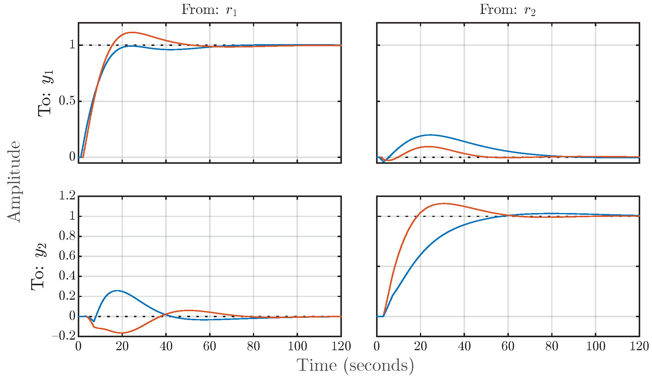
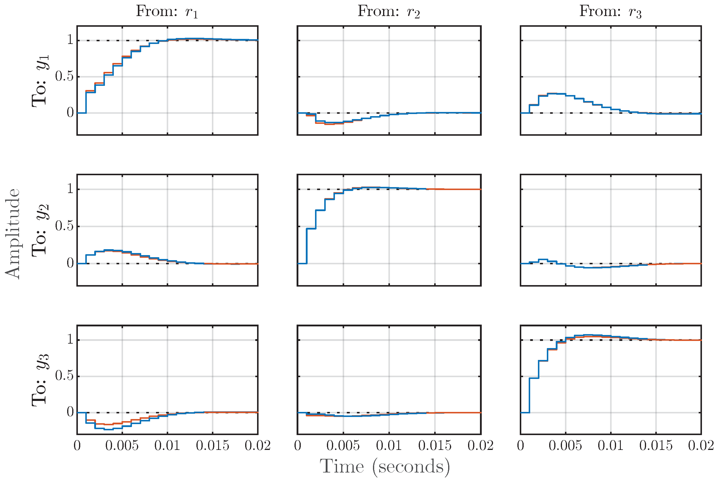
To implement the controller synthesis algorithm described in this paper, we have developed a MATLAB toolbox. The toolbox includes tools for visualizing the synthesis results, such as the figure shown in Figure 7. The toolbox also provides the synthesis of continuous controllers in the problem statement from [1].

We offer our toolbox for free use to the community under the MIT license. If you use our toolbox in your research, please consider citing this paper. Feedback, suggestions, and bug reports are welcome. The requirements for using our toolbox are as follows:

• MATLAB version above R2020a with:

  -

  Control System Toolbox;

  -

  Robust Control Toolbox;

• A convex optimization framework, such as CVX [41] or YALMIP [42]:

  -

  CVX is more conservative and has a slightly larger number of settings;

  -

  YALMIP is faster;

• An SDP solver, such as SDPT3 4.0 [43] or MOSEK [44]:

  -

  SDPT3 is more stable with numerical problems;

  -

  MOSEK is faster.

The toolbox is available at the following link:

•       https://gitlab.com/konkov/mimo-pid-lmi-synthesis-toolbox

or it can be cloned directly using the following command:

•     git clone [email protected]:konkov/mimo-pid-lmi-synthesis-toolbox.git

The Potential Numerical Problems

The numerical stability problem in algorithms is quite extensive and well known. It is associated with the fact that in any computer calculations, floating-point numbers are used, which have a constant relative error but varying absolute error. This problem is thoroughly discussed in [45].

For example, when checking the controllability of a control system model using the Kalman criterion and employing double-precision numbers, the algorithm may indicate that a control system model, which is real-controllable, appears to be uncontrollable. This discrepancy is linked to the precision of determining the matrix rank when working with floating-point numbers. When using double-precision numbers (64 bits, with a 52-bit mantissa), two numbers separated by a distance less than $2^{-52}$ are considered identical. Moreover, such a plant model will be controllable, for instance, if numbers with quadruple-precision floating-point representation are used (128 bits, with a 112-bit mantissa).

Our algorithm works with the frequency responses of transfer functions, so if the condition numbers of these responses are large, numerical problems are inevitable. We recommend initiating the controller synthesis by checking the controllability of the plant model using the Kalman criterion. If the plant model is real-controllable but the algorithm indicates an incomplete rank of the controllability matrix, scaling of the model should be conducted.

7. Numerical Examples

We present two numerical examples in which we synthesize a discrete MIMO PID controller for an LTV plant model. In both examples, we apply loop shaping to achieve a trade-off between the performance and robust stability margin of the closed-loop system. We do not delve into a detailed analysis of the presented examples but briefly emphasize the key points. All the examples presented here, along with several additional ones, are available in our toolbox. They can be easily reproduced and thoroughly explored.

7.1. Example 1

We begin with an example of the Wood–Berry binary distillation column described in [46]. This example is widely used in works dedicated to the synthesis of MIMO PID controllers. To fully demonstrate our methodology, we artificially introduce a parameter ${\delta }_n$ into the plant model. This parameter can be interpreted as uncertainties in the measured parameters or sensor faults (in the case of delay). This parametrization corresponds to the form of an uncertain model (5). Thus, some model parameters will change by a factor of two, which is significant. This way, we obtain an array of two continuous transfer functions, where s denotes the Laplace transform variable:

$$P_n\left(s\right)=\left[\begin{array}{cc}{\displaystyle \frac{12.8exp(-{\delta }_{n}s)}{16.7s+1}}& {\displaystyle \frac{-18.9exp(-3s)}{{\delta }_{n}21s+1}}\\ {\displaystyle \frac{6.6exp(-7s)}{{\delta }_{n}10.9s+1}}& {\displaystyle \frac{-{\delta }_{n}19.4exp(-3s)}{14.4s+1}}\end{array}\right],{\delta }_n\in \{1,2\}.$$

(37)

Following this, we discretize each model in the array using the ZOH method with a sample time of $T_s=0.1$ s, resulting in an array of discrete transfer functions $P_n\left(z\right)$ in the form of (6). We intentionally chose such a large sampling time. The controllability matrix of all plant models in the array is of full rank.

The results of the optimization process are shown in Figure 9, Figure 10 and Figure 11. It required six iterations to reach the optimal solution. The computation, performed using YALMIP and SDPT3 4.0 in the native MATLAB R2023b on an Apple Silicon M2 MAX SoC (System-on-Chip), took approximately 40 s.

Solving the system of LMIs (36) at $N_k=400$ (31) frequencies through the CCP, we obtain the discrete MIMO PID controller in the form of (7) with the following parameters:

$$K_P=\left[\begin{array}{c}\begin{array}{cc}\hfill 0.1246& \hfill -0.0298\\ \hfill 0.0017& \hfill -0.0340\end{array}\end{array}\right],K_I=\left[\begin{array}{c}\begin{array}{cc}\hfill 0.0182& \hfill -0.0008\\ \hfill 0.0047& \hfill -0.0038\end{array}\end{array}\right],K_D=\left[\begin{array}{c}\begin{array}{cc}\hfill -0.0016& \hfill 0.0059\\ \hfill -0.0018& \hfill -0.0019\end{array}\end{array}\right].$$

We place particular emphasis on Figure 11, which illustrates the singular values of the transfer function array (Section 3.3) of the synthesized digital control system and their shape functions (Section 4.2). Here, the following performance criteria are defined (Section 3.4): $S_{\max }=T_{\max }=1.3$, $Q_{\max }=0.25$. The shape functions $b_S\left(\omega \right)$ and $b_Q\left(\omega \right)$ are constants. The shape function $b_T\left(\omega \right)$ is a constant only for $\omega \in {\Omega }_L\cup {\Omega }_C$ (14); at high frequencies, it serves as the robustness bound (20). We do not impose any restrictions on $W_n\left(z\right)$, but one can see in Figure 11 the effect of the input external perturbation on the control performance. The key point here is that all these constraints are simultaneously satisfied for all transfer functions in the array, even considering that certain model parameters (37) change by a factor of two. This is clearly visible in Figure 11.

Regarding the trade-off between performance and robustness (Section 4.3), we have achieved a very large robustness margin while maintaining the reasonable performance of the closed-loop control system. The robustness area (21) is $A_R=4.78$, and the performance area (27) is $A_P=0.044$ (with ${\omega }_0={10}^{-3}$ rad/s). The control loops are also well-decoupled (Section 4.6), as evident from both Figure 10 and Figure 11.

7.2. Example 2

With this example, we aim to illustrate the advantages of directly synthesizing a discrete controller in a digital control system, as discussed in Section 1.4 (approach 2). The objective is to synthesize a digital control system in which the steady state is achieved within a relatively small number of samples, for example, within 10. Furthermore, we showcase the synthesis of a MIMO PID controller on a non-square plant model. This example was sourced from the MATLAB guide (https://www.mathworks.com/help/robust/ug/specify-lmi-system-at-the-command-line.html URL accessed on 6 March 2024) and was slightly modified by us. The matrix $C_n$ is parameterized by the variables $a_n$ and $b_n$, which can be interpreted both as uncertainties (5) and as values of ${\theta }_n$ in the LPV model (4) in the case of linear interpolation between time points. Below is the array of matrices for the continuous-time plant model. The plant model has $m=4$ inputs, $q=3$ outputs, and six states:

$$A=\left[\begin{array}{c}\begin{array}{cccccc}\hfill -0.0872& \hfill 0.0520& \hfill 0.0747& \hfill 0.1078& \hfill -0.0969& \hfill 0.0101\\ \hfill -0.0558& \hfill -0.1084& \hfill 0.1891& \hfill 0.0252& \hfill 0.1064& \hfill -0.0035\\ \hfill -0.0262& \hfill -0.1754& \hfill -0.1545& \hfill -0.0214& \hfill 0.0092& \hfill -0.2419\\ \hfill 0.0609& \hfill -0.1074& \hfill 0.0131& \hfill -0.2558& \hfill 0.2321& \hfill 0.0239\\ \hfill -0.0717& \hfill 0.0358& \hfill -0.1419& \hfill 0.1704& \hfill -0.2653& \hfill -0.1428\\ \hfill -0.1294& \hfill -0.0675& \hfill 0.1698& \hfill 0.1676& \hfill -0.0365& \hfill -0.1773\end{array}\end{array}\right],$$

$$B=\left[\begin{array}{c}\begin{array}{cccc}0& 89.98& -21.3& 98.35\\ 0& -30.01& 0& -29.77\\ -103.22& 0& -104.31& 114.37\\ 0& -34.51& -27.01& -53.16\\ -41.89& 101.28& -43.81& 0\\ 0& 0& -40.87& 0\end{array}\end{array}\right],a_n=\{1,1.05\},b_n=\{1,1.1\},$$

$$C_n=\left[\begin{array}{c}\begin{array}{cccccc}{a}_n·0.9707& a_n·0.951& \hfill 0.7059& \hfill b_n·1.458& \hfill -1.2371& \hfill 0.3174\\ 0& 0& \hfill 1.4158& \hfill 0.0475& \hfill -2.1935& \hfill 0.4136\\ a_n·-0.4383& a_n·0.6489& \hfill -1.6045& \hfill b_n·1.7463& \hfill -0.3334& \hfill -0.5771\end{array}\end{array}\right].$$

Similar to Example 1 (Section 7.1), we discretize each model in the array using the ZOH method, but now we utilize a sampling time of $T_s=0.001$ s. This results in an array of discrete transfer functions $P_n\left(z\right)$ in the form of (6). The controllability matrix of all plant models in the array is of full rank. The loops of the plant model are strongly coupled, as indicated by the RGA value (28) at zero frequency ($z=1$) for the first model in the array:

$$\mathrm{RGA}\left(P_1\left(1\right)\right)=\left[\begin{array}{c}\begin{array}{cccc}\hfill 0.0120& \hfill 0.2825& \hfill 1.1801& \hfill -0.4746\\ \hfill -0.5586& \hfill 0.4709& \hfill 2.4159& \hfill -1.3281\\ \hfill 0.6219& \hfill 0.1935& \hfill -2.5969& \hfill 2.7815\end{array}\end{array}\right].$$

The results are shown in Figure 12 and Figure 13.

To solve the system of LMIs in (36) with $N_k=300$, it required 11 iterations of the CCP. The optimization process on the same device and with the same software as in Example 1 (Section 7.1) took approximately 150 s. As a result, we obtained the discrete MIMO PID controller in the form of (7) with the following parameters:

$$\begin{array}{c}{K}_P=\left[\begin{array}{c}\begin{array}{ccc}\hfill -5.0392& \hfill -5.5404& \hfill 6.6605\\ \hfill -0.7234& \hfill -1.9489& \hfill -0.3424\\ \hfill -1.7436& \hfill 5.4253& \hfill -2.4762\\ \hfill -2.6610& \hfill 0.6851& \hfill 1.1269\end{array}\end{array}\right],K_I=\left[\begin{array}{c}\begin{array}{ccc}\hfill -0.9715& \hfill 0.2322& \hfill 0.6826\\ \hfill -0.3079& \hfill -0.1449& \hfill -0.1045\\ \hfill -0.3156& \hfill -0.2505& \hfill -0.4292\\ \hfill -0.1806& \hfill 0.0134& \hfill 0.0423\end{array}\end{array}\right],\\ K_D=\left[\begin{array}{c}\begin{array}{ccc}\hfill 0.0042& \hfill 0.0030& \hfill -0.0019\\ \hfill 0.0004& \hfill 0.0003& \hfill -0.0000\\ \hfill -0.0019& \hfill -0.0015& \hfill 0.0012\\ \hfill 0.0010& \hfill 0.0008& \hfill -0.0005\end{array}\end{array}\right].\end{array}$$

The step responses of the synthesized digital MIMO control system are shown in Figure 12. We have achieved the set goal, with approximately 10 samples required for the system to reach a steady state.

The singular values of the transfer function array (Section 3.3) of the synthesized digital control system and their shape functions (Section 4.2) are shown in Figure 13. For this example, the following performance criteria are defined (Section 3.4): $S_{\max }=T_{\max }=1.4$, $Q_{\max }=10$. The shape functions $b_S\left(\omega \right)$ and $b_Q\left(\omega \right)$ are constants. The shape function $b_T\left(\omega \right)$ is a constant only for $\omega \in {\Omega }_L\cup {\Omega }_C$ (14); at high frequencies, it serves as the robustness bound (20). We again do not impose any constraints on $W_n\left(z\right)$. In Figure 13, one can observe the minimal impact of the external input perturbations on the control performance. All specified constraints are simultaneously satisfied for all transfer functions in the array. The control loops are also well-decoupled (Section 4.6), as evident from both Figure 12 and Figure 13.

Here, we have a more balanced trade-off (Section 4.3) between performance and robustness compared to Example 1 (Section 7.1). The robustness area (21) is $A_R=202.4247$, and the performance area (27) is $A_P=821.33$ (with ${\omega }_0={10}^{-4}$ rad/s). Please note that the axes in Figure 13 are logarithmic.

8. Discussion

We only considered the singular values of transfer functions and did not discuss their phases. The concept of phases in MIMO transfer functions is more complex, and the theory of phases for SISO transfer functions cannot be directly applied to the MIMO case. However, in recent times, a theory of phases for MIMO transfer functions has begun to be developed. It is possible that in future works, we will enhance our synthesis algorithm by incorporating considerations of phases in MIMO transfer functions.

Indeed, PID controllers of various types enable the solution of the vast majority of practical problems. However, our proposed methodology enables tuning any controller with a fixed structure. It is only necessary to derive the SLFS function, similar to the approach outlined in Appendix B.

In fact, our methodology can also be applied to synthesizing a controller for a nonlinear plant model or even without having a plant model at all. Ultimately, when synthesizing a controller from a plant model, only a set of singular values (gains) at different frequencies is required. In the case of a linear plant model, these singular values are obtained using the transfer function when computing the frequency response. A nonlinear plant model cannot be represented as a transfer function, but the set of gains can be directly computed by applying Fourier transformation to the output signals. This way, the controller synthesis can be seamlessly combined with the identification of the plant model.

9. Conclusions

We extended the synthesis method proposed by Boyd et al. in [1] to discrete time, augmenting it with the additional statement of loop shaping. We briefly touched upon the challenges arising during the discretization of a continuous controller, especially in the MIMO case. Direct synthesis in discrete time, as opposed to discretizing a continuous controller, ensures the preservation of performance and robust stability margins in a digital control system.

We synthesized an LTI controller (7) for an LTV plant model (3) represented as a transfer function array with index n (6). This approximation of the LTV plant model can be obtained using an LPV plant model (4), an uncertain plant model (5), or by simultaneously considering both. If the system of inequalities (36) has a solution on each iteration, all specified constraints will be satisfied for the entire transfer function array of the closed-loop system with an LTV plant model (3).

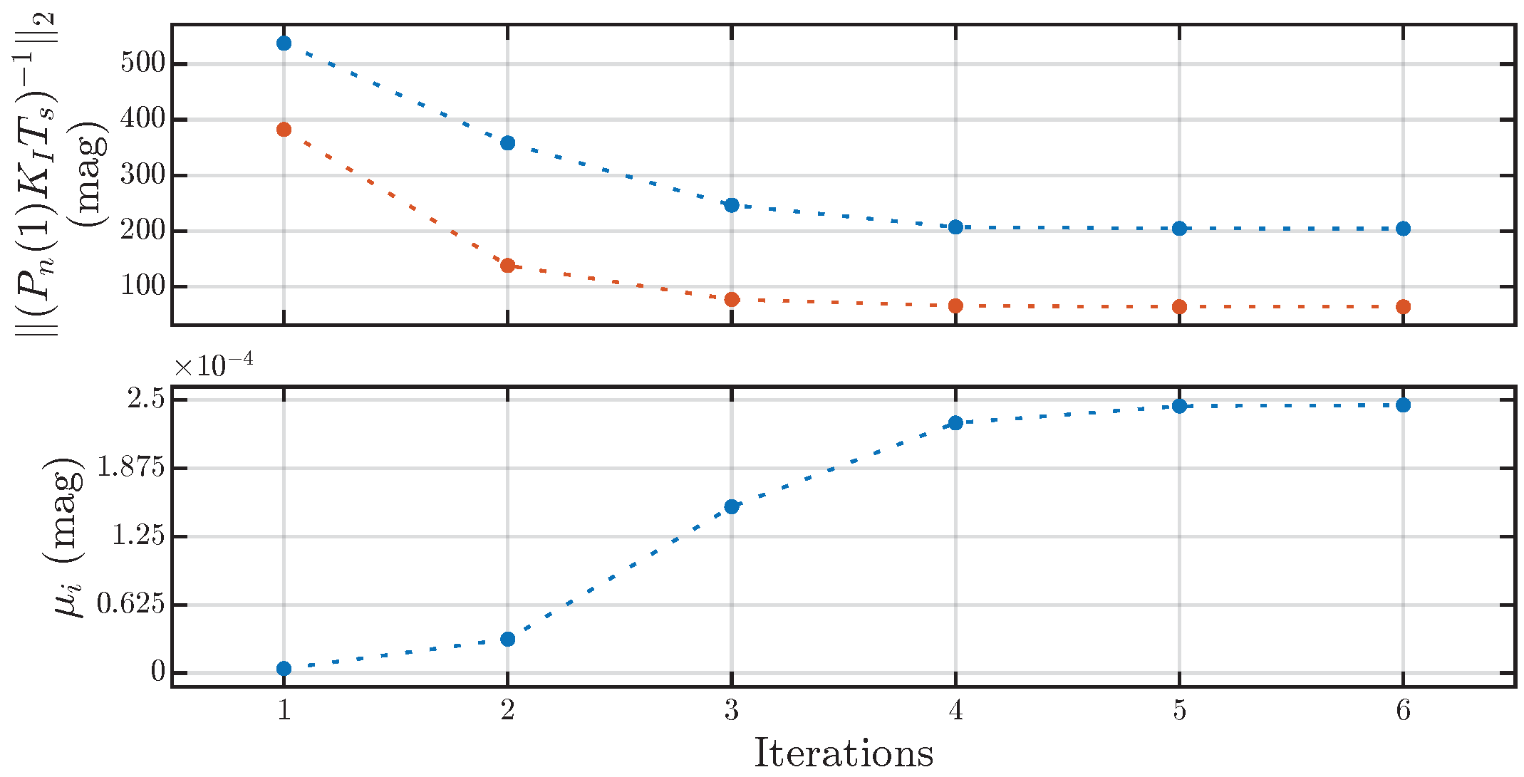
Regarding the controller derived from our algorithm, it is important to emphasize the following. We achieve an optimal controller, signifying that the closed-loop system attains maximum performance under constraints imposed on the transfer functions of the closed-loop system. This maximization of performance is realized through the iterative minimization of the static and low-frequency sensitivity (SLFS) of the closed-loop system, facilitated by the minimization of the spectral norm of the SLFS matrix (11). Ultimately, this translates into the maximization of the performance area $A_P$ (27) with a “floating” boundary represented by the performance bound $b_P\left(\omega \right)$ (26). By employing the convex-concave procedure (CCP), we obtain a locally optimal solution to the system (36) at each iteration, progressively converging toward the global optimum. Furthermore, the flexibility of the optimization algorithm enables termination at any point by adjusting the CCP stopping condition, contingent on the desired values of the performance area and performance bound.

The minimization of the spectral norm of the SLFS matrix serves dual objectives: ensuring the decoupling of control loops at low frequencies and maximizing control performance. Additionally, it results in a closed-loop system with crossover frequencies as proximate as possible, leading to nearly identical time responses for its control loops. The presence of a “floating” performance bound is considered an advantage of our methodology compared to classical loop shaping, where both bounds are strictly defined, impeding the synthesis of an optimal controller. The judicious selection of the robustness bound $b_R\left(\omega \right)$ (20) holds critical importance in digital systems, affording a sufficiently extensive robustness area and obviating the need for anti-aliasing filters in the feedback loop. By varying the robustness bound, a trade-off is struck between performance and the robust stability margin of the closed-loop system. A larger robustness area corresponds to a smaller performance area, and vice versa. We propose simple estimates for this trade-off, manifested in the form of performance and robustness bounds ($b_P\left(\omega \right)$, $b_R\left(\omega \right)$) (20), (26) and performance and robustness areas ($A_P$, $A_R$) (27), (20). To fortify robust stability, our tripartite strategy involves synthesizing over an array of models, integrating ${\mathcal{H}}_{\infty }$-norm constraints guided by the small-gain theorem, and employing loop shaping to concurrently specify a robustness bound for all models in the plant model array.

The methodology proposed in this paper was developed by us as part of the development of digital plasma magnetic control systems in tokamaks. We have used some elements from this methodology in our previous works [47,48,49,50]. Of particular note is that in [50], the controller synthesis was conducted simultaneously for an array of 20 LTI plant models, and the plasma shape controller had five inputs and six outputs. The methodology presented in this paper will continue to be used by us in the future for plasma control.

We also hope that this methodology can be applied in many other fields. Given the complexity of our method and the potentially time-consuming nature of programming the algorithm, we offer a ready-to-use MATLAB toolbox for convenience. Moreover, we have strived to thoroughly explicate all nuances of the methodology, intending to simplify its comprehension for readers to the utmost.

Limitations of This Study

This paper is theoretical in nature and proposes a new methodology for synthesizing discrete MIMO PID controllers. The numerical examples provided serve solely to illustrate some of the capabilities of the proposed method. Our study was not aimed at comparing MIMO PID to other controller types, nor was it aimed at comparing our synthesis method to existing ones. We provide a ready-to-use toolbox to allow researchers to independently compare their own synthesis methods with our method.

A separate study dedicated to comparing different controller types may be conducted in the future. Due to the complex nature of discrete controller synthesis methods in MIMO control systems with well-coupled control loops and the potential difficulty of such investigations, it is desirable to involve experts in each type of controller under study. However, even with such involvement, such research may only apply to certain classes of plants. There are no universally effective controllers, nor are there universal methods for synthesizing them. A controller is simply a tool used to solve a specific control problem for a real plant. Comparing different types of controllers for a single class of plants is not sufficient and may not reveal the full potential of each design. Ultimately, the aim of any controller design method is to create a reliable control system that satisfies specified performance requirements while also possessing the necessary robust stability margins. In addition, the physical implementation aspects of digital controllers must be considered. Many complex control algorithms may experience difficulties operating in real time on existing hardware. It is also important to take into account the rationality of utilizing each type of controller, as it may not be rational to use a more complex algorithm when a simpler one could accomplish the task with only a slight decrease in performance.

Potential future research could be systematic, considering all these factors. Perhaps this could be a book, where each section is written by an expert on a specific type of controller. Additionally, objective comparison criteria for different types of controllers should be formulated for different classes of plants. We are ready to contribute our methodology for synthesizing MIMO PID controllers to such a book.

References

1. Boyd, S.; Hast, M.; Åström, K.J. MIMO PID tuning via iterated LMI restriction. Int. J. Robust Nonlinear Control 2016, 26, 1718–1731. [Google Scholar] [CrossRef]
2. Åström, K.; Hägglund, T. The future of PID control. Control Eng. Pract. 2001, 9, 1163–1175. [Google Scholar] [CrossRef]
3. Åström, K.J.; Hägglund, T. Advanced PID Control; ISA—The Instrumentation, Systems, and Automation Society: Research Triangle Park, NC, USA, 2006. [Google Scholar]
4. Soltesz, K.; Cervin, A. When is PID a good choice? IFAC-PapersOnLine 2018, 51, 250–255. [Google Scholar] [CrossRef]
5. Mohammadpour, J.; Grigoriadis, K.; Franchek, M.; Wang, Y.Y.; Haskara, I. LPV decoupling for control of multivariable systems. Int. J. Control 2011, 84, 1350–1361. [Google Scholar] [CrossRef]
6. Baár, T.; Bauer, P.; Luspay, T. Parameter Varying Mode Decoupling for LPV systems. IFAC-PapersOnLine 2020, 53, 1219–1224. [Google Scholar] [CrossRef]
7. Davison, E. Multivariable tuning regulators: The feedforward and robust control of a general servomechanism problem. IEEE Trans. Autom. Control 1976, 21, 35–47. [Google Scholar] [CrossRef]
8. Penttinen, J.; Koivo, H. Multivariable tuning regulators for unknown systems. Automatica 1980, 16, 393–398. [Google Scholar] [CrossRef]
9. Boyd, S.P. Linear Matrix Inequalities in System and Control Theory; Number vol. 15 in SIAM Studies in Applied Mathematics; Society for Industrial and Applied Mathematics: Philadelphia, PA, USA, 1994. [Google Scholar]
10. Zheng, F.; Wang, Q.G.; Lee, T.H. On the design of multivariable PID controllers via LMI approach. Automatica 2002, 38, 517–526. [Google Scholar] [CrossRef]
11. Feng, Z.Y.; Guo, H.; She, J.; Xu, L. Weighted sensitivity design of multivariable PID controllers via a new iterative LMI approach. J. Process Control 2022, 110, 24–34. [Google Scholar] [CrossRef]
12. Guo, H.; Feng, Z.Y.; She, J. Discrete-time multivariable PID controller design with application to an overhead crane. Int. J. Syst. Sci. 2020, 51, 2733–2745. [Google Scholar] [CrossRef]
13. Solgi, Y.; Fatehi, A.; Nikoofard, A.; Shariati, A. Design of optimal PID controller for multivariable time-varying delay discrete-time systems using non-monotonic Lyapunov-Krasovskii approach. J. Frankl. Inst. 2021, 358, 6634–6665. [Google Scholar] [CrossRef]
14. Doyle, J.; Stein, G. Multivariable feedback design: Concepts for a classical/modern synthesis. IEEE Trans. Autom. Control 1981, 26, 4–16. [Google Scholar] [CrossRef]
15. Safonov, M.; Laub, A.; Hartmann, G. Feedback properties of multivariable systems: The role and use of the return difference matrix. IEEE Trans. Autom. Control 1981, 26, 47–65. [Google Scholar] [CrossRef]
16. McFarlane, D.; Glover, K. A loop-shaping design procedure using H/sub infinity / synthesis. IEEE Trans. Autom. Control 1992, 37, 759–769. [Google Scholar] [CrossRef]
17. Genç, A.U.; Impram, S.T. A State-Space Algorithm for Designing H-inf Loop Shaping PlD Controllers. IFAC Proc. Vol. 2003, 36, 281–286. [Google Scholar] [CrossRef]
18. Hast, M.; Astrom, K.; Bernhardsson, B.; Boyd, S. PID design by convex-concave optimization. In Proceedings of the 2013 European Control Conference (ECC), Zurich, Switzerland, 17–19 July 2013; pp. 4460–4465. [Google Scholar] [CrossRef]
19. Franklin, G.F.; Powell, J.D.; Workman, M.L. Digital Control of Dynamic Systems, 3rd ed.; Addison-Wesley: Menlo Park, CA, USA, 1998. [Google Scholar]
20. Kotel’nikov, V.A. On the transmission capacity of ’ether’ and wire in electric communications. Usp. Fiz. Nauk 2006, 176, 762–770, Peprint. The original paper was published in 1933. [Google Scholar] [CrossRef]
21. Åström, K.J.; Wittenmark, B. Computer-Controlled Systems: Theory and Design, 3rd ed.; Prentice Hall Information and System Sciences Series; Prentice Hall: Upper Saddle River, NJ, USA, 1997. [Google Scholar]
22. Chida, Y.; Nishimura, T. Discretization Method of Continuous-Time Controllers Based on Frequency Response Fitting. Sice J. Control. Meas. Syst. Integr. 2008, 1, 299–306. [Google Scholar] [CrossRef]
23. Watkins, D.S. Fundamentals of Matrix Computations, 3rd ed.; Pure and Applied Mathematics; Wiley: Hoboken, NJ, USA, 2010. [Google Scholar]
24. Ragazzini, J.R.; Zadeh, L.A. The analysis of sampled-data systems. Trans. Am. Inst. Electr. Eng. Part II Appl. Ind. 1952, 71, 225–234. [Google Scholar] [CrossRef]
25. Tsipkin, Y.Z. Theory of intermittent regulation. Avtom. Telemekhanika 1949, 10, 189–224. [Google Scholar]
26. Doetsch, G.; Herschel, R. Anleitung zum Praktischen Gebrauch der Laplace-Transformation und der Z-Transformation, 5th ed.; korrigierter nachdr. der 3., neu neubearb. aufl ed.; Oldenbourg: München, Germany, 1985. [Google Scholar]
27. Lyons, R.G. Understanding Digital Signal Processing, 2nd ed.; Prentice Hall PIR: Upper Saddle River, NJ, USA, 2004. [Google Scholar]
28. Zames, G. On the input-output stability of time-varying nonlinear feedback systems Part one: Conditions derived using concepts of loop gain, conicity, and positivity. IEEE TRansactions Autom. Control 1966, 11, 228–238. [Google Scholar] [CrossRef]
29. Skogestad, S.; Postlethwaite, I. Multivariable Feedback Control: Analysis and Design, 2nd ed.; John Wiley: Hoboken, NJ, USA, 2005. [Google Scholar]
30. Zhou, K.; Doyle, J.C. Essentials of Robust Control; Prentice Hall: Upper Saddle River, NJ, USA, 1998. [Google Scholar]
31. Boyd, S.P.; Barratt, C.H. Linear Controller Design: Limits of Performance; Prentice Hall Information and System Sciences Series; Prentice Hall: Englewood Cliffs, NJ, USA, 1991. [Google Scholar]
32. Apkarian, P.; Gahinet, P. A convex characterization of gain-scheduled H/sub / controllers. IEEE Trans. Autom. Control 1995, 40, 853–864. [Google Scholar] [CrossRef]
33. Briat, C. Linear Parameter-Varying and Time-Delay Systems: Analysis, Observation, Filtering & Control; Advances in Delays and Dynamics; Springer: Berlin/Heidelberg, Germany, 2015; Volume 3. [Google Scholar] [CrossRef]
34. Tóth, R.; Heuberger, P.S.C.; Van den Hof, P.M.J. LPV system identification using series expansion models. In Linear Parameter-Varying System Identification; WORLD SCIENTIFIC: Singapore, 2011; pp. 259–294. [Google Scholar] [CrossRef]
35. Duan, G.R.; Yu, H.H. LMIs in Control Systems; CRC Press: Boca Raton, FL, USA, 2013. [Google Scholar] [CrossRef]
36. Youla, D.; Jabr, H.; Bongiorno, J. Modern Wiener-Hopf design of optimal controllers–Part II: The multivariable case. IEEE Trans. Autom. Control 1976, 21, 319–338. [Google Scholar] [CrossRef]
37. Glover, K.; Sefton, J.; Mcfarlane, D. A Tutorial on Loop Shaping using H-Infinity Robust Stabilization. IFAC Proc. Vol. 1990, 23, 117–126. [Google Scholar] [CrossRef]
38. Phillips, C.L.; Parr, J.M.; Riskin, E.A. Signals, Systems, and Transforms, 4th ed.; Pearson/Prentice Hall: Upper Saddle River, NJ, USA, 2008. [Google Scholar]
39. Boyd, S.P.; Vandenberghe, L. Convex Optimization; Cambridge University Press: Cambridge, UK; New York, NY, USA, 2004. [Google Scholar]
40. Lipp, T.; Boyd, S. Variations and extension of the convex–concave procedure. Optim. Eng. 2016, 17, 263–287. [Google Scholar] [CrossRef]
41. Grant, M.; Boyd, S. CVX: Matlab Software for Disciplined Convex Programming, Version 2.1. 2014. Available online: http://cvxr.com/cvx (accessed on 6 March 2024).
42. Lofberg, J. YALMIP: A toolbox for modeling and optimization in MATLAB. In Proceedings of the 2004 IEEE International Conference on Robotics and Automation (IEEE Cat. No.04CH37508), Taipei, Taiwan, 2–4 September 2004; pp. 284–289. [Google Scholar] [CrossRef]
43. Tütüncü, R.H.; Toh, K.C.; Todd, M.J. Solving semidefinite-quadratic-linear programs using SDPT3. Math. Program. 2003, 95, 189–217. [Google Scholar] [CrossRef]
44. ApS, M. The MOSEK Optimization Toolbox for MATLAB Manual, Version 10.1.27. 2024. Available online: https://docs.mosek.com/10.1/toolbox.pdf (accessed on 6 March 2024).
45. Higham, N.J. Accuracy and Stability of Numerical Algorithms, 2nd ed.; Society for Industrial and Applied Mathematics: Philadelphia, PA, USA, 2002. [Google Scholar]
46. Wood, R.; Berry, M. Terminal composition control of a binary distillation column. Chem. Eng. Sci. 1973, 28, 1707–1717. [Google Scholar] [CrossRef]
47. Konkov, A.E.; Mitrishkin, Y.V.; Korenev, P.S.; Patrov, M.I. Robust Cascade LMI Design of MIMO Control System for Plasma Position, Current, and Shape Model with Time-Varying Parameters in a Tokamak. IFAC-PapersOnLine 2020, 53, 7344–7349. [Google Scholar] [CrossRef]
48. Mitrishkin, Y.V.; Korenev, P.S.; Konkov, A.E.; Kartsev, N.M. Suppression of Vertical Plasma Displacements by Control System of Plasma Unstable Vertical Position in D-Shaped Tokamak. Autom. Remote Control 2022, 83, 579–599. [Google Scholar] [CrossRef]
49. Konkov, A.E.; Mitrishkin, Y.V. Comparison Study of Power Supplies in Real-Time Robust Control Systems of Vertical Plasma Position in Tokamak. IFAC-PapersOnLine 2022, 55, 327–332. [Google Scholar] [CrossRef]
50. Konkov, A.E.; Korenev, P.S.; Mitrishkin, Y.V.; Balachenkov, I.M.; Kiselev, E.O. Real-Time Plasma Magnetic Control System with Equilibrium Reconstruction Algorithm in the Feedback for the Globus-M2 Tokamak. Plasma Phys. Rep. 2023, 49, 1552–1559. [Google Scholar] [CrossRef]
51. Deadman, E.; Relton, S.D. Taylor’s theorem for matrix functions with applications to condition number estimation. Linear Algebra Its Appl. 2016, 504, 354–371. [Google Scholar] [CrossRef]
52. Hjørungnes, A. Complex-Valued Matrix Derivatives: With Applications in Signal Processing and Communications; Cambridge University Press: Cambridge, UK, 2011. [Google Scholar]
Figure 1. An example of a 3 × 2 MIMO PID controller with 2 inputs ( e 1 , e 2 ) and 3 outputs ( u 1 , u 2 , u 3 ).
Mathematics 12 00810 g001
Figure 2. A block diagram of a basic digital control system.
Mathematics 12 00810 g002
Figure 3. A control system with output multiplicative uncertainty in the plant model.
Mathematics 12 00810 g003
Figure 4. A control system with output additive uncertainty in the plant model.
Mathematics 12 00810 g004
Figure 5. Classical feedback interconnection of reference tracking control system.
Mathematics 12 00810 g005
Figure 6. Examples of three shape functions.
Mathematics 12 00810 g006
Figure 7. An example illustrating loop shaping. The singular values of the transfer functions L ( z ) , S ( z ) , and T ( z ) of the MIMO control system. The performance area and robustness area are shaded.
Mathematics 12 00810 g007
Figure 8. The singular values of the transfer functions L ( z ) , S ( z ) , and T ( z ) of the MIMO control system in Figure 7 with the addition of the condition number for T ( z ) .
Mathematics 12 00810 g008
Figure 9. The results of the CCP for Example 1. The convergence of the local optimum μ i to the optimum μ is demonstrated, along with the variation in the spectral norm of the SLFS matrix. The blue dashed line corresponds to P 1 ( z ) , whereas the red line corresponds to P 2 ( z ) .
Mathematics 12 00810 g009
Figure 10. Example 1: Step responses of the synthesized digital MIMO control system, structured according to the diagram in Figure 5. The blue line corresponds to P 1 ( z ) , whereas the red line corresponds to P 2 ( z ) .
Mathematics 12 00810 g010
Figure 11. Example 1: Singular values of the transfer function array L n ( z ) , S n ( z ) , Q n ( z ) , and T n ( z ) of the synthesized digital MIMO control system. The performance area and robustness area are shaded. The shape functions are indicated by dashed lines.
Mathematics 12 00810 g011
Figure 12. Example 2: Step responses of the synthesized digital MIMO control system, organized according to the diagram in Figure 5. The blue line corresponds to P 1 ( z ) , whereas the red line corresponds to P 2 ( z ) .
Mathematics 12 00810 g012
Figure 13. Example 2: Singular values of the transfer function array L n ( z ) , S n ( z ) , Q n ( z ) , and T n ( z ) of the synthesized digital MIMO control system. The performance area and robustness area are shaded. The shape functions are indicated by dashed lines.
Mathematics 12 00810 g013
Disclaimer/Publisher’s Note: The statements, opinions and data contained in all publications are solely those of the individual author(s) and contributor(s) and not of MDPI and/or the editor(s). MDPI and/or the editor(s) disclaim responsibility for any injury to people or property resulting from any ideas, methods, instructions or products referred to in the content.