Article

Fractional-Order Model-Free Adaptive Control with High Order Estimation

School of Computer Science, Fudan University, Shanghai 200433, China
*
Author to whom correspondence should be addressed.
Mathematics 2024, 12(5), 784; https://doi.org/10.3390/math12050784
Submission received: 8 January 2024 / Revised: 31 January 2024 / Accepted: 5 February 2024 / Published: 6 March 2024

Abstract

:
This paper concerns an improved model-free adaptive fractional-order control with a high-order pseudo-partial derivative for uncertain discrete-time nonlinear systems. Firstly, a new equivalent model is obtained by employing the Grünwald–Letnikov (G-L) fractional-order difference of the input in a compact-form dynamic linearization. Then, the pseudo-partial derivative (PPD) is derived using a high-order estimation algorithm, which provides more PPD information than the previous time. A discrete-time model-free adaptive fractional-order controller is proposed, which utilizes more past input–output data information. The ultimate uniform boundedness of the tracking errors are demonstrated through formal analysis. Finally, the simulation results demonstrate the effectiveness of the proposed method.

1. Introduction

Recently, the model-free adaptive control (MFAC) method has attracted extensive attention; it does not need the specific dynamic characteristics of the control system, only input and output data [1]. Thanks to its fewer identification parameters and fewer calculations, as well as its wide range of applications, MFAC plays an important role in many fields and applications [2].
Different from the existing stability analysis for discrete-time (stochastic) systems [3,4,5], the main idea of MFAC is to use the concept of a pseudo-gradient to replace the general discrete-time nonlinear system with a series of dynamic linear time-varying models. In MFAC, the dynamic linear time-varying model has three main forms, namely, compact-form dynamic linearization (CFDL) [6], partial-form dynamic linearization (PFDL) [7], and full-form dynamic linearization (FFDL) [8]. In particular, by utilizing only input–output data information, equivalent models can be derived by means of the concept of a pseudo-partial derivative (PPD). Thus, the learning law can be established by treating the PPD as a time-varying parameter [9,10].
Using a virtual equivalent dynamic linearization data model, the time-varying PPD estimation algorithm was designed in [11], where the internal stability of the FFDL linearization-based MFAC scheme was rigorously presented. In [12], a new type of MFAC method based on an adaptive forgetting factor was proposed. In [13], by taking the affine structure of the ultra-local model and the extended state observer (ESO), a local PFDL-based ESO-MFAC was proposed to improve control performance. In order to make the MFAC scheme have a better performance, a PID-like MFAC with discrete (ESO) sparked interest in [14]. It is worth pointing out that the above-mentioned work did not consider high-order PPD estimation.
High-order MFAC is an important branch of MFAC which uses more information to further improve control performance. In [15], a high-order estimation algorithm was used to estimate the value of PPD. An improved high-order MFAC method was proposed in [16], which not only considered more control knowledge than the previous time, but also used more information from the previous time in the estimation algorithm.
Fractional-order control is popular in controlling nonlinear systems [17]. In [18], a data driven model has been established and a discrete time fractional order reaching law was studied. In [19], a fractional order data-driven model was proposed, which related the first variation of the output signal with the fractional order variation of the input one. A fractional data-driven model was presented in [20], where the instantaneous gain from the fractional output variation to the input one was computed by means of a fuzzy inference system.
These observations motivate our current study. The main contributions of this paper can be summarized into two aspects: (1) both the error and its rate of change are introduced in the control input criterion function, which incorporates a fractional-order operator. Three weighting coefficients are executed to enhance the system capacity of track abrupt signals and mitigate sudden external disturbance; (2) by using the high-order PPD estimation scheme based on previous input and output data, a fractional-order MFAC with high order estimation to enhance convergence is developed.
The rest of this paper is organized as follows: some preliminaries and the problem formulation are presented in Section 2. The data-driven control algorithm is given in Section 3. A theoretical analysis of the enhanced convergent condition is derived in Section 4. Section 5 provides numerical simulations to illustrate the validity of the designed method. Finally, some conclusions are drawn in Section 6.

2. System Description

In this paper, we consider the following uncertain discrete-time nonlinear system:
y ( k + 1 ) = f ( k , y ( k ) , , y ( k n y ) , u ( k ) , , u ( k n u ) ) ,
where k { 0 , 1 , T } indexes the discrete time and T is the terminal time instant. u ( k ) R is the control input at time instant k and y ( k ) R is the system output at time instant k. n y , n u N are two unknown positive integers.
Definition 1 
([21]). The fractional discrete approximation of the G-L derivative for u ( k ) is defined as
Δ n u ( k ) = 1 h n v = 0 k ( 1 ) v n v u ( k v ) ,
where n R is the fractional order, R is the set of real numbers, h is set to 1 as a sampling time, and k N is a number of samples for which the approximation of the derivative is calculated.
The fractional binomial term in (2) can be obtained from the following relation:
n v = 1 for v = 0 n ( n 1 ) ( n v + 1 ) v ! for v > 0
The following assumptions are considered for the system (1).
Assumption 1. 
There exist positive constants u M and y M such that | Δ n u ( k ) | u M and | y ( k ) | y M .
Assumption 2. 
For any k { 0 , 1 , , T } , the nonlinear function f ( · , , · ) satisfies the Lipschitz condition, that is,
| Δ y ( k + 1 ) | l | Δ n u ( k ) | ,
where Δ y ( k + 1 ) = y ( k + 1 ) y ( k ) , l is a Lipschitz constant.
Remark 1. 
The above assumptions are rather standard, and they are taken for granted by several schemes for the control of discrete-time systems. Assumption 1 gives a limit on the system input and output change rate. From a practical point of view, Assumption 2 implies that the output variation depends linearly on the input variation.
By virtue of the second assumption, the dynamic model of (1) can be expressed as
Δ y ( k + 1 ) = ϕ ( k ) Δ n u ( k ) ,
where ϕ ( k ) satisfies | ϕ ( k ) | l . ϕ ( k ) establishes a dynamic relationship between the input and output data of the system. Therefore, the rapid identification of ϕ ( k ) becomes particularly crucial. This issue will be addressed in the next section. In this paper, we exclusively address the case of n ( 0 , 1 ] .
Remark 2. 
When n = 1 , Δ u n ( k ) degenerates to the conventional integer-order cases. ϕ ( k ) aligns with the standard pseudo-partial derivative in CFDL. For n ( 0 , 1 ) , due to the short-memory characteristics of a fractional-order operator [21], the controller compensates for more information from the previous time; therefore, the robustness of the system’s equivalent model can be enhanced. This contributes to a smoother execution of dynamic linearization, enabling a faster convergence of the estimated ϕ ^ ( k ) to the desired ϕ ( k ) .
Assumption 3. 
For any k { 0 , 1 , T } , the PPD satisfies ε ϕ ( k ) (or ϕ ( k ) ε ), where ε is a relatively small positive constant.
Remark 3. 
Most of the plants, in practice, can satisfy Assumption 3. Its practical meaning is obvious, that is, the plant output should increase (or decrease) when the corresponding control input increases.

3. Design of Model-Free Adaptive Fractional-Order Controller

The following improved calculation criteria are considered:
J ( u ( k ) ) = e T ( k + 1 ) Δ e T ( k + 1 ) Q e e ( k + 1 ) Δ e ( k + 1 ) + λ Δ n u ( k ) 2 ,
where
e ( k + 1 ) = y d ( k + 1 ) y ( k + 1 )
and
Δ e ( k + 1 ) = e ( k + 1 ) e ( k )
represent the tracking error and its rate of change, respectively. y d ( k ) is the desired trajectory. Q e 1 and Q e 2 R are positive weight coefficients in Q e = d i a g { Q e 1 , Q e 2 } . λ > 0 is a penalty factor, which is used in order to limit the control input variation.
Remark 4. 
In the input criterion function (6), the first term is the square of the output error. The second term is the rate of change of the error at two adjacent moments. This is used to reduce the impact of excessive changes in the criterion function calculation by the output data.
Substituting (5) into the criterion function (6), we can obtain
J ( u ( k ) ) = Q e 1 y d ( k + 1 ) y ( k ) ϕ ( k ) Δ n u ( k ) 2 + Q e 2 y d ( k + 1 ) y ( k ) ϕ ( k ) Δ n u ( k ) e ( k ) 2 + λ Δ n u ( k ) 2 .
Through calculating, this yields
1 2 J ( u ( k ) ) u ( k ) = Q e 1 ϕ ( k ) ( y d ( k + 1 ) y ( k ) ϕ ( k ) Δ n u ( k ) ) Q e 2 ϕ ( k ) ( y d ( k + 1 ) y ( k ) ϕ ( k ) Δ n u ( k ) e ( k ) ) + λ Δ n u ( k ) .
Using the optimal technique, one can have
Δ n u ( k ) = ρ ϕ ( k ) ( ( Q e 1 + Q e 2 ) Δ y d ( k + 1 ) + Q e 1 e ( k ) ) λ + | Q e 1 + Q e 2 ϕ ( k ) | 2 ,
where, as a step factor, ρ is designed to make the controller more universal [22].
Note that
Δ n u ( k ) = v = 1 k ( 1 ) v n v u ( k v ) + u ( k ) .
Thus, an improved model-free adaptive fractional-order controller (I-MFAFOC) can be expressed by
u ( k ) = ρ ϕ ( k ) ( ( Q e 1 + Q e 2 ) Δ y d ( k + 1 ) + Q e 1 e ( k ) ) λ + | Q e 1 + Q e 2 ϕ ( k ) | 2 v = 1 k ( 1 ) v n v u ( k v ) .
Remark 5. 
Unlike other high-order algorithms designed based on the control input [13,14,16], the I-MFAFOC algorithm (10) uses y d ( k + 1 ) to update the control input u ( k ) . On the other hand, compared to the algorithm in [16], the improved algorithm does not need to set the weight coefficients for the previous control inputs u ( k v ) , v = 1 , , k .
Since ϕ ( k ) is unknown, the following universal criteria function with the estimated parameter are defined:
J ( ϕ ( k ) ) = Δ y ( k ) ϕ ( k ) Δ n u ( k 1 ) 2 + μ ϕ ( k ) ϕ ^ ( k 1 ) 2 ,
where μ is the weight factor. ϕ ^ ( k ) is the estimated value of ϕ ( k ) . Equation (11) indicates that the target-constrained input should be minimized, while the tracking error converges to a minimum; this implies that ϕ ^ ( k ) will converge to ϕ ( k ) .
In this paper, for enhancing tracking performance, a high-order parameter estimation algorithm for PPD (HOPPD) is proposed here by updating the criterion function (11) as follows:
J ( ϕ ( k ) ) = Δ y ( k ) ϕ ( k ) Δ n u ( k 1 ) 2 + μ ϕ ( k ) j = 1 m α j ϕ ^ ( k j ) 2 ,
where m N + is the high-order degree and α j are weighting coefficients with j = 1 m α j = 1 .
Based on the derivation of (12), as below, and J ( ϕ ( k ) ) / ϕ ( k ) = 0 , the estimation algorithm is expressed by (13)
ϕ ^ ( k ) = Δ n u ( k 1 ) Δ y ( k ) μ + Δ n u ( k 1 ) 2 + μ η μ + Δ n u ( k 1 ) 2 j = 1 m α j ϕ ^ ( k j ) ,
where η is the step length to make the algorithm more flexible [22].
To ensure that the dynamic linearization model is always true, the following reset algorithm is applied:
ϕ ^ ( k ) = ϕ ^ ( 1 ) , if ϕ ^ ( k ) ε or | Δ n u ( k 1 ) | ε .
ϕ ^ ( k ) = ϕ ^ ( k 1 ) + η Δ n u ( k 1 ) μ + Δ n u ( k 1 ) 2 ( Δ y ( k ) ϕ ^ ( k 1 ) Δ n u ( k 1 ) ) , 2 k < m ϕ ^ ( k ) = Δ n u ( k 1 ) Δ y ( k ) μ + Δ n u ( k 1 ) 2 + μ η μ + Δ n u ( k 1 ) 2 j = 1 m α j ϕ ^ ( k j ) , k m
u ( k ) = ρ ϕ ^ ( k ) ( ( Q e 1 + Q e 2 ) Δ y d ( k + 1 ) + Q e 1 e ( k ) ) λ + | Q e 1 + Q e 2 ϕ ^ ( k ) | 2 v = 1 k ( 1 ) v n v u ( k v ) .
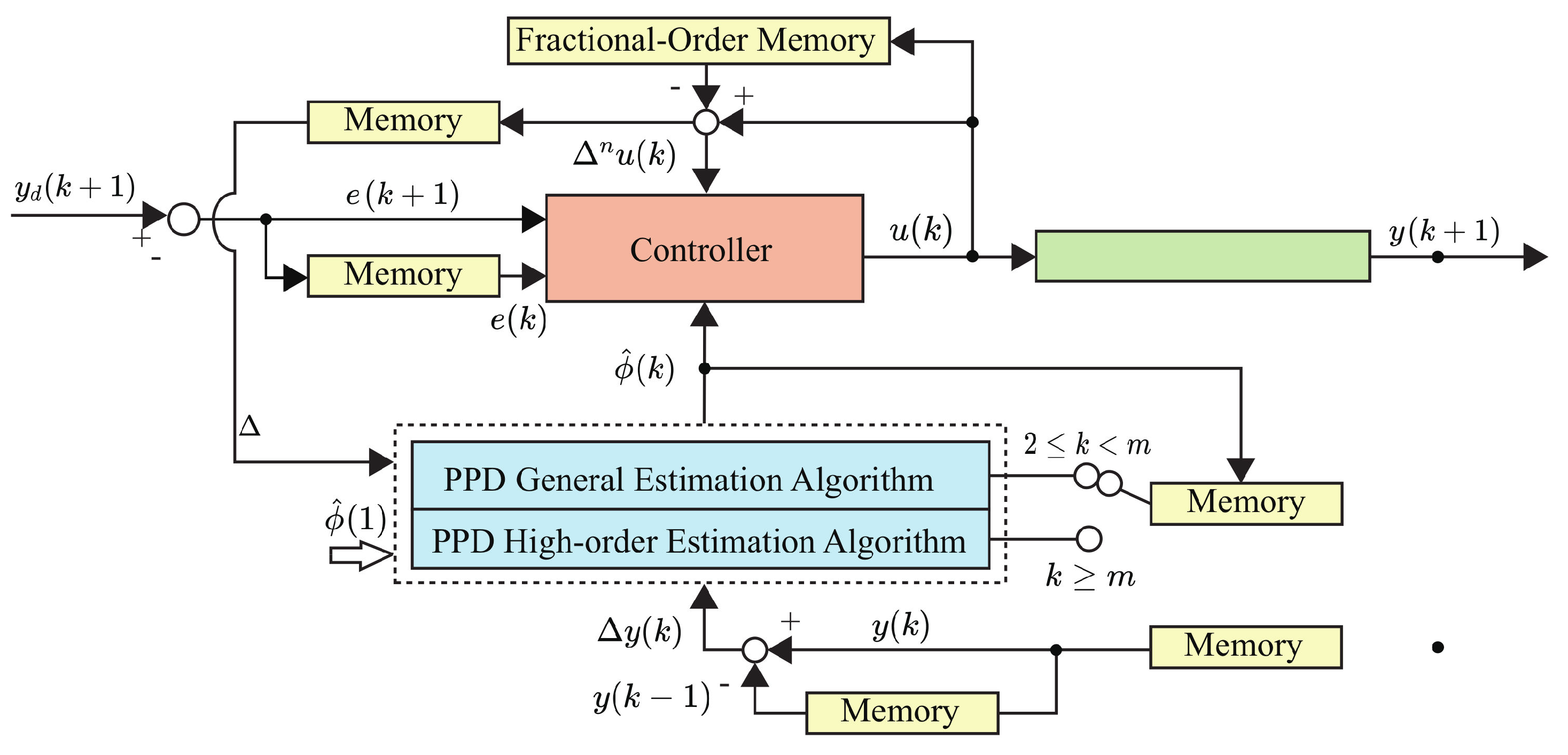
Therefore, the overall control strategy of the proposed high-order PPD-based improved model-free adaptive fractional-order controller (HOPPD-I-MFAFOC) is delineated in Equations (14)–(16). The controller diagram is depicted in Figure 1 with the following two key points. (1) The PPD is derived using a high-order estimation algorithm. (2) The fractional-order controller is used to provide a better performance.
In comparison with traditional MFAC, HOPPD-I-MFAFOC incorporates more historical input and output data, enriching the gain parameters by involving ϕ ^ ( k ) due to the inclusion of a fractional-order and high-order algorithm.
Remark 6. 
For practical realization, the number of samples taken into consideration has to be reduced to the predefined number L { 0 , 1 , , N } and N < T in the experiment [23].
Remark 7. 
In the first instance, an initial value needs to be assigned to ϕ ^ ( 1 ) . Since the calculation of ϕ ^ ( k ) relies on the previous m instances, it can only be computed when k m . Therefore, the high-order estimation algorithm (15) is applied for k m . However, in the case of 2 k < m , where no previous instances are available, the original estimation algorithm in (16) is utilized.
Remark 8. 
The application of weighting coefficients α j in the high-order estimation algorithm (15) is analogous to the use of a forgetting factor. Consequently, they can set α 1 α 2 α m .

4. Convergence Analysis

The following theorem can be obtained.
Theorem 1. 
For system (1), if Assumptions 1 and 2 hold, then for k { 0 , 1 , 2 , , T } , ϕ ^ ( k ) is bounded with η ( 0 , 1 ] .
Proof. 
When 2 k < m , the original estimation algorithm in (15) can be rewritten as
ϕ ^ ( k ) = 1 η | Δ n u ( k 1 ) | 2 μ + | Δ n u ( k 1 ) | 2 ϕ ^ ( k 1 ) + η Δ n u ( k 1 ) Δ y ( k ) μ + | Δ n u ( k 1 ) | 2 .
From the assumptions of system (1), one has that
< η Δ n u ( k 1 ) Δ y ( k ) μ + | Δ n u ( k 1 ) | 2 < ,
whenever | Δ n u ( k 1 ) Δ y ( k ) | < since 0 < μ < μ + | Δ n u ( k 1 ) | 2 . Thus, using the triangle inequality, we have
| Δ n u ( k 1 ) Δ y ( k ) | l | Δ n u ( k 1 ) | 2 ,
consequently, according to Assumption 2, we have
Δ n u ( k 1 ) Δ y ( k ) μ + | Δ n u ( k 1 ) | 2 l | Δ n u ( k 1 ) | 2 μ + | Δ n u ( k 1 ) | 2 l a 1 < .
It is worth noting that | Δ n u ( k 1 ) | 2 μ + Δ n u ( k 1 ) 2 is monotonically increasing and bounded about Δ n u ( k 1 ) . Set
a 1 = sup k [ 0 , T ] | Δ n u ( k 1 ) | 2 μ + | Δ n u ( k 1 ) | 2 .
Then, there is a relation that satisfies
0 1 η | Δ n u ( k 1 ) | 2 μ + | Δ n u ( k 1 ) | 2 1 η a 2 < 1 ,
where
a 2 = inf k [ 0 , T ] | Δ n u ( k 1 ) | 2 μ + | Δ n u ( k 1 ) | 2 .
When k m , by taking the absolute value on both sides, we obtain from (15) that
| ϕ ^ ( k ) | = Δ n u ( k 1 ) 2 Δ y ( k ) μ + Δ n u ( k 1 ) 2 + μ η j = 1 m α j ϕ ^ ( k j ) μ + Δ n u ( k 1 ) 2 l a 1 + η 1 | Δ n u ( k 1 ) | 2 μ + Δ n u ( k 1 ) 2 j = 1 m α j ϕ ^ ( k j ) l a 1 + ( η η 2 a 2 ) j = 1 m α j ϕ ^ ( k j ) ,
where ( η η 2 a 2 ) ( 0 , 1 ) , since the boundedness of j = 1 m α j ϕ ^ ( k j ) has been demonstrated before. Therefore, ϕ ^ ( k ) is uniformly ultimately bounded, as demonstrated in the above proof. Given that ϕ ( k ) is bounded, it follows that ϕ ^ ( k ) is bounded as well. Additionally, the PPD estimation error ϕ ˜ ( k ) = ϕ ^ ( k ) ϕ ( k ) is also bounded. The proof is completed. □
Theorem 2. 
For system (1) with the help of the HOPPD-I-MFAFOC scheme (15) and (16), if Assumptions 1 and 2 are satisfied and
λ > ε ρ Q e 1 2 Q e 1 + Q e 2 ,
then an error convergence rate 0 < M < 1 is introduced, ensuring that the tracking error e ( k ) converges to zero as k with 0 < ρ 1 .
Proof. 
Using model (5), we have
| e ( k + 1 ) | = Δ y d ( k + 1 ) ϕ ^ ( k ) Δ n u ( k ) + e ( k ) .
Substituting Equation (9) into the Equation (25), this yields
| e ( k + 1 ) | = | Δ y d ( k + 1 ) + e ( k ) ρ ϕ ( k ) ϕ ^ ( k ) ( ( Q e 1 + Q e 2 ) Δ y d ( k + 1 ) + Q e 1 e ( k ) ) λ + | Q e 1 + Q e 2 ϕ ^ ( k ) | 2 | ( 1 ρ Q e 1 ϕ ( k ) ϕ ^ ( k ) λ + | Q e 1 + Q e 2 ϕ ^ ( k ) | 2 ) e ( k ) 1 ρ Q e 1 ϕ ( k ) ϕ ^ ( k ) λ + | Q e 1 + Q e 2 ϕ ^ ( k ) | 2 e ( k ) .
From Assumption 2 and the reset algorithm (15), the inequality ϕ ( k ) ϕ ^ ( k ) 0 is obtained. Furthermore, one has that
[ λ ± Q e 1 + Q e 2 ϕ ^ ( k ) ] 2 = λ + ( Q e 1 + Q e 2 ) [ ϕ ^ ( k ) ] 2 ± 2 λ ( Q e 1 + Q e 2 ) ϕ ^ ( k ) 0 ,
and consequently
2 λ ( Q e 1 + Q e 2 ) | ϕ ^ ( k ) | λ + ( Q e 1 + Q e 2 ) [ ϕ ^ ( k ) ] 2 .
Then,
1 ρ Q e 1 ϕ ( k ) | ϕ ^ ( k ) | λ + | Q e 1 + Q e 2 ϕ ^ ( k ) | 2 e ( k ) 1 ρ Q e 1 ϕ ( k ) 2 λ ( Q e 1 + Q e 2 ) e ( k ) ( 1 ε d ) 2 e ( k 1 ) ( 1 ε d ) 3 e ( k 2 ) ( 1 ε d ) k e ( 1 ) ,
where
d = ρ Q e 1 2 λ m i n ( Q e 1 + Q e 2 )
is a bounded constant. Therefore, there exists a constant
M = ( 1 ε d ) = sup k [ 0 , T ] 1 ρ Q e 1 ϕ ( k ) | ϕ ^ ( k ) | λ m i n + | Q e 1 + Q e 2 ϕ ^ ( k ) | 2
that represents the rate of error convergence. The proof is completed. □
Theorem 3. 
For k 0 , 1 , 2 , , T , u ( k ) and y ( k ) are bounded, indicating that the closed-loop system is BIBO stable.
Proof. 
The following equation is obtained from Equation (9):
| Δ n u ( k ) | = ρ ϕ ( k ) ( ( Q e 1 + Q e 2 ) Δ y d ( k + 1 ) + Q e 1 e ( k ) ) λ + | Q e 1 + Q e 2 ϕ ( k ) | 2 ρ Q e 1 2 λ ( Q e 1 + Q e 2 ) | e ( k ) |
d | ( e ( k ) | .
Apply absolute values to both sides of Equation (2):
| Δ n u ( k ) | = v = 0 k ( 1 ) v n v u ( k v ) .
Let
ψ ( v ) = ( 1 ) v n v
be a function of v, where
1 < { ψ ( 1 ) , ψ ( 2 ) , ψ ( 3 ) , , ψ ( k ) } < 0 .
The following relation can be derived from (27) and (29):
| Δ n u ( k ) | = | ψ ( 0 ) ψ ( 1 ) ψ ( 2 ) ψ ( k 1 ) u ( k ) u ( k 1 ) u ( k 2 ) u ( 1 ) | d | ( e ( k ) | .
Note that
u ( k ) = ψ ( 0 ) u ( k ) + ψ ( 1 ) u ( k 1 ) ψ ( 1 ) u ( k 1 ) ψ ( 0 ) u ( k ) + ψ ( 1 ) u ( k 1 ) + ψ ( 1 ) u ( k 1 ) ψ ( 0 ) u ( k ) + ψ ( 1 ) u ( k 1 ) + ψ ( 2 ) u ( k 2 ) + ψ ( 1 ) u ( k 1 ) + ψ ( 2 ) u ( k 2 ) | Δ n u ( k ) | + ψ ( 1 ) u ( k 1 ) + ψ ( 2 ) u ( k 2 ) + + ψ ( k 1 ) u ( 1 ) d ( e ( k ) + ψ ( 1 ) u ( k 1 ) + ψ ( 2 ) u ( k 2 ) + + ψ ( k 1 ) u ( 1 ) d | ( e ( k ) | + ψ ( 1 ) u ( k 1 ) + ψ ( 2 ) u ( k 2 ) + + ψ ( k 1 ) u ( 1 ) d | ( e ( k ) | + p = 1 k 1 u ( k p ) ,
where { | ψ ( 1 ) | , | ψ ( 2 ) | , , | ψ ( k ) | } < 1 . This sequence, through a recursive relation, expresses | u ( k ) | as a function of the input and error at previous time steps. According to Equation (31), the following sequence of inequalities is obtained at other times:
| u ( k 1 ) | d | ( e ( k 1 ) | + p = 2 k 1 u ( k p ) | u ( k 2 ) | d | ( e ( k 2 ) | + p = 3 k 1 u ( k p ) | u ( 2 ) | d | ( e ( 2 ) | + u ( 1 ) .
By combining the inequality sequences (31) and (32), (31) can be reformulated as follows:
| u ( k ) | d | e ( k ) | + d | e ( k 1 ) | + p = 2 k 1 u ( k p ) d | e ( k ) | + d | e ( k 1 ) | + + d | e ( 1 ) | + u ( 1 ) d ( M k 1 | e ( 1 ) | + M k 2 | e ( 1 ) | + + M | e ( 1 ) | + u ( 1 ) < d M 1 M | e ( 1 ) | + u ( 1 ) .
This implies that u ( k ) is bounded.The proof is completed. □

5. Numerical Examples

In this section, to validate the effectiveness of the proposed method, two numerical examples are presented.
Example 1. 
An unknown plant replaced by a differencing equation is represented as follows:
y ( k + 1 ) = 0.3 y ( k ) + 0.6 y ( k 1 ) + 0.6 sin ( π u ( k ) ) + 0.3 sin ( 3 π u ( k ) ) + 0.1 sin ( 5 π u ( k ) ) .
The tracking trajectory is given as
y d ( k ) = 2 , 0 k 150 4 , 150 < k 300 .
The controller parameters are λ = 0.1 , ρ = 0.2 , μ = 0.01 , and η = 0.8 . The predefined number is fixed at L = 100 . The fractional-order is set as n = 0.8 . The high-order estimation is configured with m = 3 , and the weighting coefficients are α 1 = 0.4 , α 2 = 0.4 , and α 3 = 0.2 . The high-order estimation algorithm commences at k = 4 . The initial PPD is uniformly set as ϕ ^ ( 1 ) = 10 for all controllers. Moreover, the weighting coefficients is chosen as Q e = d i a g { 1 , 0.1 } .
Figure 2 illustrates the tracking performance of each controller in response to the given reference signal. Table 1 presents a comparison of the Sum Square Error (SSE) and Sum Square Control (SSC) between fractional-order and tuned integer order. The results indicate that the I-MFAFOC method shortens the response time and reduces SSE to a certain extent, but requires an increased control effort. The HOPPD-MFAFOC method reduces the overshoot of the tracking signal and decreases SSC to a certain extent, but increases SSE. The HOPPD-I-MFAFOC method achieves a reduction in SSE and SSC, to a certain extent, simultaneously. Moreover, all three fractional-order control methods mentioned above significantly outperform the traditional MFAC method.
Example 2. 
To demonstrate the effectiveness of the proposed control method in tracking smooth reference signals, a comparative experiment was conducted as follows. The system (36) contains time-varying parameters and uncertain disturbance κ ( k ) :
y ( k + 1 ) = sin ( y ( k ) ) + u ( k ) [ 5 + cos ( y ( k ) u ( k ) ) ] + κ ( k ) .
Define the desired trajectory as
y d ( k + 1 ) = 0.5 sin ( k / 20 ) + 0.5 sin ( k / 40 ) .
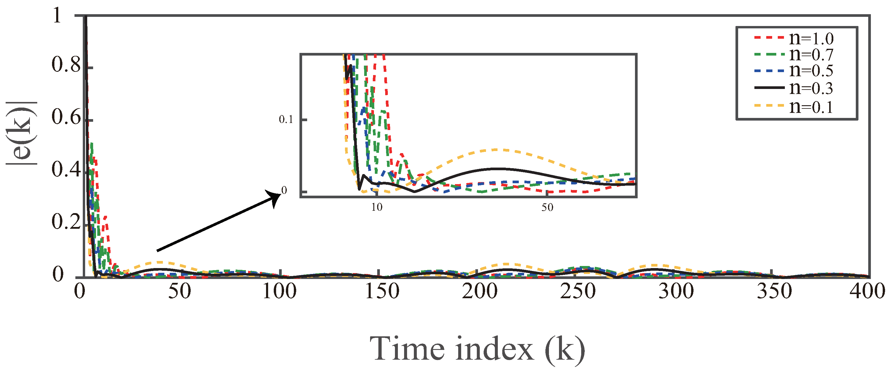
The HOPPD-I-MFAFOC method is applied to control the system (37) in simulation experiments. The controller parameters are λ = 0.01 , ρ = 0.9 , μ = 0.01 , and η = 0.8 . The predefined number is set to L = 100 . A comparison between fractional-order and tuned integer order with respect to SSE and SSC is presented in Table 2. The tracking performance of each controller is shown in Figure 3.
The fractional order is chosen as n = 0.3 . The order of the high-order estimation is specified as m = 3 , with weighting coefficients α 1 = 0.4 , α 2 = 0.4 , a n d α 3 = 0.2 . The high-order estimation algorithm commences at k = 4 . The initial PPD is uniformly set as ϕ ^ ( 1 ) = 10 for all controllers, and the weight factor is defined as Q e = d i a g { 1 , 0.2 } .
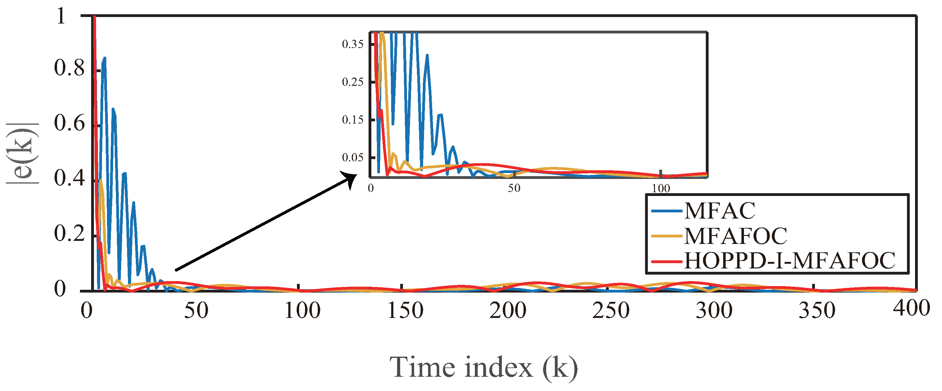
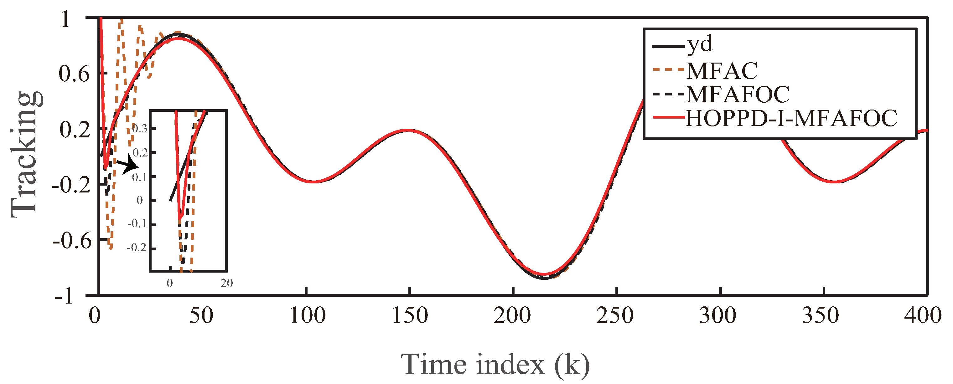
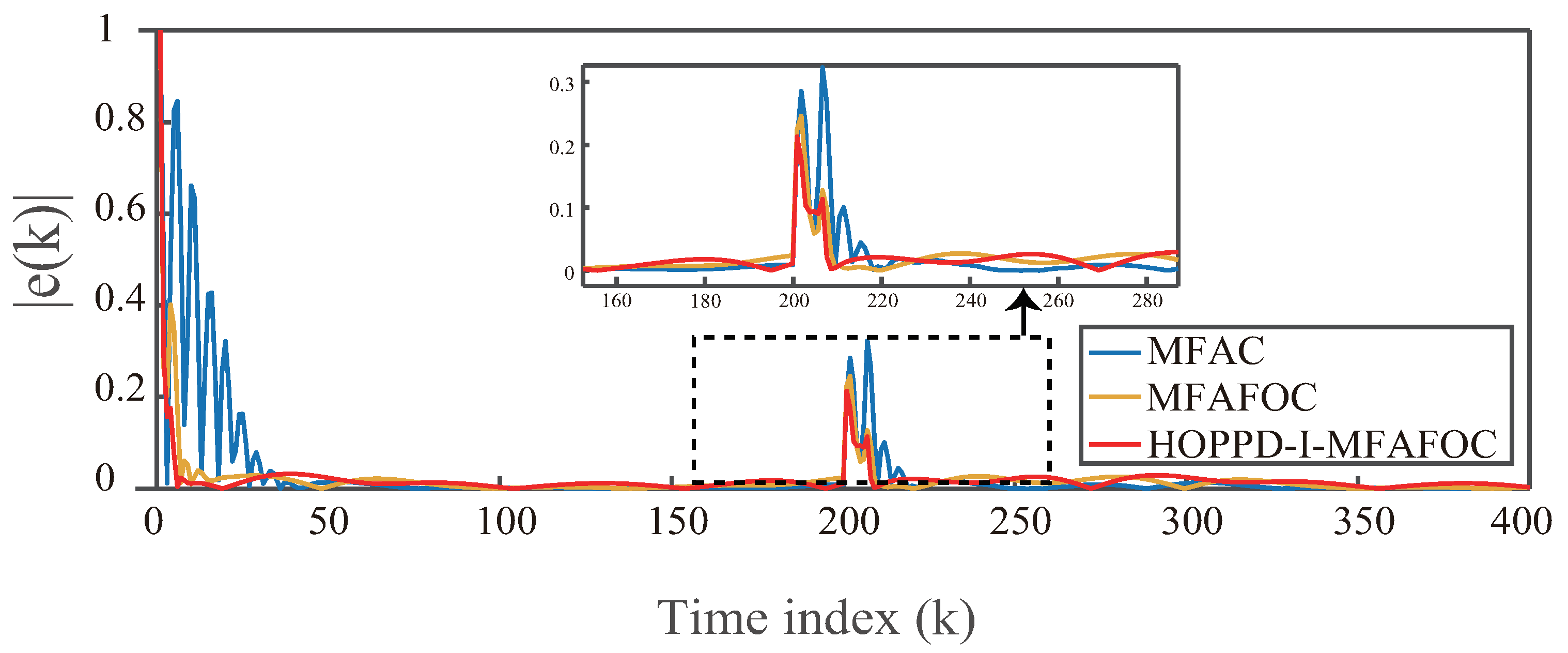
Figure 4 and Figure 5 provide a trajectory tracking comparison among the MFAC, MFAFOC, and HOPPD-I-MFAFOC methods for the ideal case. The MFAC parameters are set to λ = 0.01 , ρ = 0.5 , μ = 0.01 , and η = 0.5 , demonstrating superior performance. Additionally, performance enhancements are evident when comparing SSE and SSC indices in Table 3. The results indicate that HOPPD-I-MFAFOC exhibits a 19.46% reduction in SSE and a 13.18% reduction in SSC compared to MFAFOC in tracking the target signal.
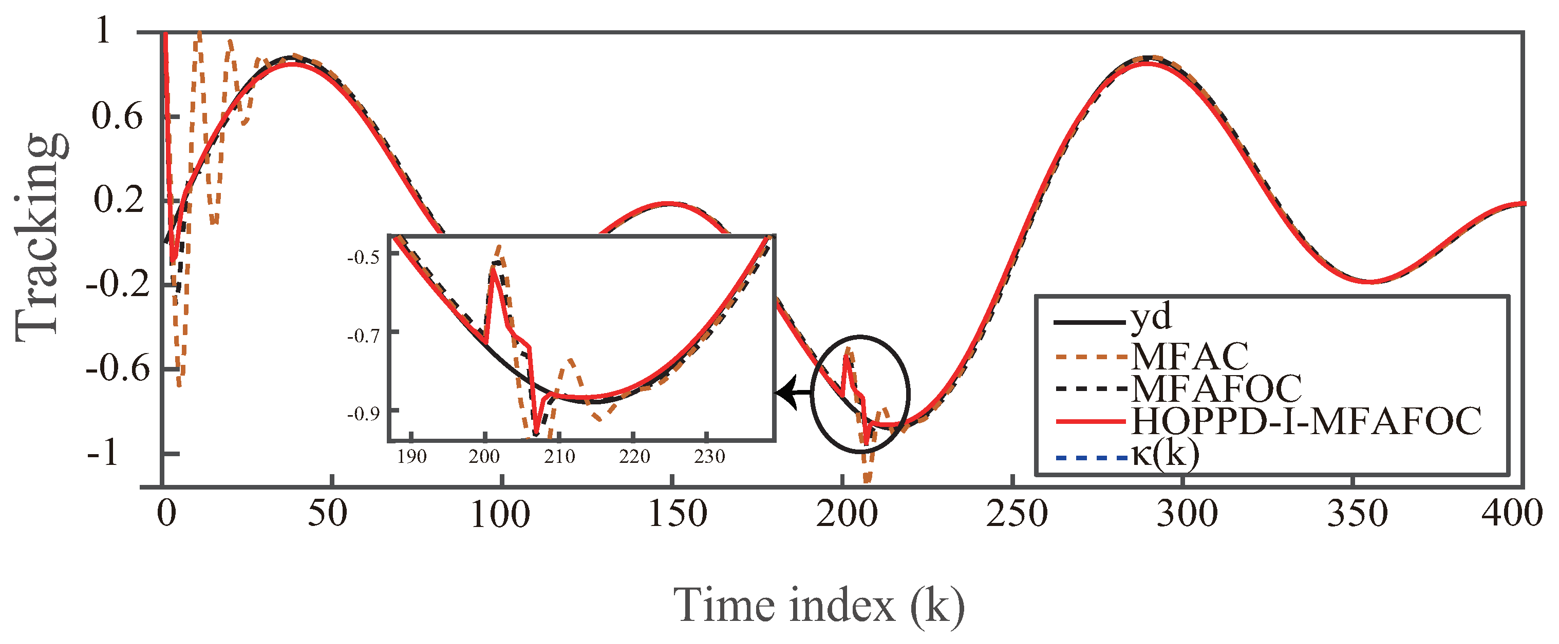
Figure 6 and Figure 7 demonstrate the robustness of the method, verified by introducing an uncertain disturbance based on repeating the experiment described above. The experiment illustrates the enhanced robustness of the new control method. Additionally, Table 4 provides a comparison between the MFAC, MFAFOC, and HOPPD-I-MFAFOC methods in terms of SSC and SSE for the case with a disturbance. The results show that HOPPD-I-MFAFOC exhibits a 26.43% reduction in SSE and a 9.71% reduction in SSC compared to MFAFOC in tracking the target signal.
6. Conclusions

In this paper, based on the compact-form fractional order dynamic linearization, an improved controller was applied to uncertain discrete-time nonlinear systems. Utilizing the fractional-order short-memory characteristics enhances the tracking performance of the output and the system’s disturbance rejection capability. Additionally, the introduction of the tracking error rate of change and the incorporation of a high-order estimation algorithm for PPD complement each other, further improving the controller’s performance. Our future work may focus on improving the MFAILC protocol, enabling the use of the fractional-order in the iterative axis and elsewhere in MFAC.

Author Contributions

Methodology, J.L.; Formal analysis, Z.-X.L. All authors have read and agreed to the published version of the manuscript.

Funding

This research received no external funding.

Data Availability Statement

Data is contained within the article.

Conflicts of Interest

The authors declare no conflicts of interest.

References

  1. Hou, Z.S.; Han, Z.G. Parameter estimation algorithm of nonlinear systems and its dual adaptive control. Acta Autom. Sin. 1995, 21, 12–21. [Google Scholar]
  2. Ma, Y.S.; Che, W.W.; Deng, C.; Wu, Z.G. Distributed model-free adaptive control for learning nonlinear MASs under DoS attacks. IEEE Trans. Neural Netw. Learn. Syst. 2021, 34, 1146–1155. [Google Scholar] [CrossRef] [PubMed]
  3. Zhang, C.K.; Chen, W.H.; Zhu, C.; He, Y.; Wu, M. Stability analysis of discrete-time systems with time-varying delay via a delay-dependent matrix-separation-based inequality. Automatica 2023, 156, 1111922. [Google Scholar] [CrossRef]
  4. Bao, W.; Zhu, Q.X. Stability analysis of discrete-time semi-Markov jump linear systems. IEEE Trans. Autom. Control 2020, 65, 5415–5421. [Google Scholar]
  5. Bao, W.; Zhu, Q.X.; Li, S. Stabilization of discrete-time hidden semi-Markov jump linear systems with partly unknown emission probability matrix. IEEE Trans. Autom. Control 2023, 99, 1–8. [Google Scholar]
  6. Zhang, B.; Zhang, W. Adaptive predictive functional control of a class of nonlinear systems. ISA Trans. 2006, 45, 175–183. [Google Scholar] [CrossRef] [PubMed]
  7. Hou, Z.S.; Jin, S. Model-Free Adaptive Control for a Class of Nonlinear Discrete-Time Systems Based on the Partial Form Linearization. IFAC Proc. Vol. 2008, 41, 3509–3514. [Google Scholar] [CrossRef]
  8. Li, Y.; Hou, Z.S.; Liu, X. Full form dynamic linearization based data-driven mfac for a class of discrete-time nonlinear systems. In Proceedings of the 2011 Chinese Control and Decision Conference (CCDC), Mianyang, China, 23–25 May 2011; pp. 127–132. [Google Scholar]
  9. Treesatayapun, C. Model free adaptive control with pseudo partial derivative based on fuzzy rule emulated network. In Proceedings of the 2012 International Conference on Artificial Intelligence (ICAI), Las Vegas, NV, USA, 16–19 July 2012; pp. 257–269. [Google Scholar]
  10. Chen, R.Z.; Li, Y.X.; Hou, Z.S. Distributed model-free adaptive control for multi-agent systems with external disturbances and DoS attacks. Inf. Sci. 2022, 613, 309–323. [Google Scholar] [CrossRef]
  11. Hou, Z.S.; Xiong, S. On model-free adaptive control and its stability analysis. IEEE Trans. Autom. Control 2019, 64, 4555–4569. [Google Scholar] [CrossRef]
  12. Liao, Y.; Du, T.; Jiang, Q. Model-free adaptive control method with variable forgetting factor for unmanned surface vehicle control. Appl. Ocean. Res. 2019, 93, 101945. [Google Scholar] [CrossRef]
  13. Chi, R.; Hui, Y.; Zhang, S.; Huang, B.; Hou, Z.S. Discrete-time extended state observer-based model-free adaptive control via local dynamic linearization. IEEE Trans. Ind. Electron. 2020, 67, 8691–8701. [Google Scholar] [CrossRef]
  14. Wang, C.; Huo, X.; Ma, K.; Ji, R. Pid-like model free adaptive control with discrete extended state observer and its application on an unmanned helicopter. IEEE Trans. Ind. Inform. 2023, 19, 11265–11274. [Google Scholar] [CrossRef]
  15. Liu, F.; Wang, Z.; Gao, F. Improved high order model-free adaptive iterative learning control with disturbance compensation and enhanced convergence. Comput. Model. Eng. Sci. 2023, 134, 343–355. [Google Scholar]
  16. Xu, J.; Lin, N.; Chi, R.; Li, X. High-order model-free adaptive iterative learning control. Trans. Inst. Meas. Control 2023, 45, 1886–1895. [Google Scholar] [CrossRef]
  17. Podlubny, I. Fractional Differential Equations; Academic Press: San Diego, CA, USA, 1999. [Google Scholar]
  18. Chidentree, T.; Aldo, J.M. Discrete-time fractional-order control based on data-driven equivalent model. Appl. Soft Comput. 2020, 96, 106633. [Google Scholar]
  19. Aldo, J.; Chidentree, T. Fractional data-driven model for stabilization of uncertain discrete-time nonlinear systems. J. Frankl. Inst. 2022, 359, 9690–9702. [Google Scholar]
  20. Chidentree, T.; Aldo, J. Model-free adaptive control based on fractional input-output data model. Appl. Sci. 2022, 12, 11168. [Google Scholar]
  21. Zieliński, A.; Sierociuk, D. Stability of discrete fractional order state space systems. IFAC Proc. Vol. 2006, 39, 505–510. [Google Scholar] [CrossRef]
  22. Hou, Z. Model Free Adaptive Control: Theory and Applications; CRC Press: Boca Raton, FL, USA, 2013. [Google Scholar]
  23. Wei, Y.H.; Chen, Y.Q.; Cheng, S.; Wang, Y. A note on short memory principle of fractional calculus. Fract. Calc. Appl. Anal. 2017, 20, 1382–1404. [Google Scholar] [CrossRef]
Figure 1. Block diagram of the proposed HOPPD-I-MFAFOC.
Mathematics 12 00784 g001
Figure 2. Comparison of the ability of different controllers to handle abrupt reference signals [16,20].
Mathematics 12 00784 g002
Figure 3. Comparison of different fractional orders when employing the HOPPD-I-MFAFOC method.
Mathematics 12 00784 g003
Figure 4. Trajectory tracking results for MFAC, MFAFOC, and HOPPD-I-MFAFOC [19,23].
Mathematics 12 00784 g004
Figure 5. Comparison of the tracking error convergence among MFAC, MFAFOC, and HOPPD-I-MFAFOC [19,23].
Mathematics 12 00784 g005
Figure 6. Tracking performance with disturbance κ ( k ) [19,23].
Mathematics 12 00784 g006
Figure 7. Tracking error convergence with disturbance κ ( k ) [19,23].
Mathematics 12 00784 g007
Table 1. A comparison of SSE and SSC among different controllers.
nCONTROLLERSSESSC
n = 1.0MFAC55.43601.2655
n = 0.8MFAFOC30.10951.2634
n = 0.8I-MFAFOC29.8452 ↓1.2702 ↑
n = 0.8HOPPD-MFAFOC30.1924 ↑1.2514 ↓
n = 0.8HOPPD-I-MFAFOC29.9294 ↓1.2575 ↓
Table 2. A comparison of SSE and SSC for different orders using HOPPD-I-MFAFOC.
FRACTIONAL-ORDERSSESSC
0.11.32560.0313
0.31.24780.0369
0.51.39610.0448
0.71.85420.0612
1.04.82350.0582
Table 3. A comparison of SSE and SSC with different control methods. ( κ ( k ) = 0 ).
CONTROLLERSSESSC
MFAC5.19840.0759
MFAFOC [19]1.54920.0425
HOPPD-I-MFAFOC1.2478 ↓0.0369 ↓
Table 4. A comparison of SSE and SSC with different control methods. ( κ ( k ) 0 ).
CONTROLLERSSESSC
MFAC5.81120.0951
MFAFOC [19]1.85000.0546
HOPPD-I-MFAFOC1.3611 ↓0.0493 ↓
Disclaimer/Publisher’s Note: The statements, opinions and data contained in all publications are solely those of the individual author(s) and contributor(s) and not of MDPI and/or the editor(s). MDPI and/or the editor(s) disclaim responsibility for any injury to people or property resulting from any ideas, methods, instructions or products referred to in the content.