On Stochastic Representations of the Zero–One-Inflated Poisson Lindley Distribution

Abstract

A zero–one-inflated Poisson Lindley distribution has been introduced recently as an alternative to the zero–one-inflated Poisson distribution for describing count data with a substantial number of zeros and ones. Several stochastic representations of the zero–one-inflated Poisson Lindley distribution and their equivalence to some well-known distributions under some conditions are presented. Using these stochastic representations, the distributional properties such as the nth moments, as well as the conditional distributions are discussed. These stochastic representations can be used to explain the relationship between two or more distributions. Several likelihood ratio tests are developed and examined for the presence of one-inflation and fixed rate parameters. The likelihood ratio tests are found to be powerful and have ability to control the error rates as the sample size increases. A sample size of 1000 is acceptable and sufficient for the likelihood ratio tests to be useful.

1. Introduction

One common phenomenon in statistics is the presence of excess zeroes only. This phenomenon happens when there are more zero-valued observations than explained by the Poisson distribution. There have been numerous studies conducted in analysing count data with zero-inflation such as zero-inflated models [1,2,3,4], hurdle models [4], zero-altered models [3] and others. Young et al. [5] has provided a comprehensive review on the use of the zero-inflated models and its associated regression models. The zero-inflated models are commonly used to explain the excess zeroes by introducing an inflation parameter known as zero-inflation parameter.

Recently, the presence of excess zeros and ones in count data have been gaining attraction by researchers as they are also common in statistics. This phenomenon happens when there is an abundance of observed events that are not happening and happening only once. This phenomenon arises quite naturally depending on the questions we would like to answer. Lin and Tsai [6] have provided a list of questions that will ultimately give the observations inflated at zero and non-zero. For inflation at zero and one, asking questions about a memorable event that happened in one’s life such as the number of marriages [6] will certainly yield results that have a huge spike at zero and one because it is natural and common across time for mankind to either stay single or get married to one person at a time or in life. The phenomenon of excess zeros and ones can also be found in various fields such as medicine [6] as well as quantitative criminology [7,8].

Introducing two inflation parameters into an existing distribution to describe excess zeros and ones, respectively, is normal and extensively researched [6,7,8,9,10]. Although the zero–one-inflated Poisson distribution (ZOIP) was introduced in the late 20th century by Melkersson and Olsson [9], its stochastic representations were not explored until 17 years later by Zhang et al. [10]. The study by Zhang et al. [10] interrelates the ZOIP distribution with other known Poisson distributions such as the zero-inflated Poisson, the zero-truncated Poisson and the one-truncated Poisson distributions. Following the idea of Zhang et al. [10], this paper examines and discusses some notes on the stochastic representations for the zero–one-inflated Poisson Lindley distribution (ZOIPL) developed by Tajuddin et al. [8]. Likelihood ratio tests are also developed to investigate whether the presence of one-inflation and fixed parameters is significant.

The probability mass function (pmf) for a random variable Y following the ZOIPL distribution [8] is given as:

$$\mathrm{Pr}\left(Y=y\right)=\{\begin{array}{l}{\omega }_0+\left(1-{\omega }_0-{\omega }_1\right)\frac{{\theta }^2\left(\theta +2\right)}{{\left(\theta +1\right)}^3};y=0\\ {\omega }_1+\left(1-{\omega }_0-{\omega }_1\right)\frac{{\theta }^2\left(\theta +3\right)}{{\left(\theta +1\right)}^4};y=1\\ \left(1-{\omega }_0-{\omega }_1\right)\frac{{\theta }^2\left(\theta +y+2\right)}{{\left(\theta +1\right)}^{y+3}};y\ge 2\end{array},$$

(1)

where ${\omega }_0$ and ${\omega }_1$ explain the excess zeroes and ones, respectively, and $\theta$ is the parameter of the Poisson Lindley, $PL$ distribution [11]. The $PL$ distribution has been shown to provide a better fit than the Poisson distribution due to its ability to handle overdispersion in the data [11,12]. The parameter $\theta$ in the $PL$ distribution plays a crucial role in determining the variation in the distribution. As $\theta$ increases, the variance and the mean of the $PL$ distribution approach to an identical value, a phenomenon known as equidispersion (see [12], 2009 for further explanation). Similarly, the $ZOIPL$ distribution has also been shown to provide better model fittings over the $ZOIP$ distribution due to its ability to handle extra dispersion, of which cannot be single-handedly described by the inflation parameters in the $ZOIP$ distribution [8].

Note that, if ${\omega }_0=0$, the $ZOIPL$ distribution reduces to a one-inflated Poisson Lindley, $OIPL$ distribution with parameters ${\omega }_1$ and $\theta$, which have not been studied yet. Readers are advised to not be confused with a one-inflated-positive Poisson Lindley distribution, which was developed to cater for inflation in one-valued data in positive count data [13]. If ${\omega }_1=0$, the $ZOIPL$ distribution reduces to the zero-inflated Poisson Lindley distribution ($ZIPL$) with parameters ${\omega }_0$ and $\theta$ [14]. If both ${\omega }_0,{\omega }_1=0$, the $ZOIPL$ distribution reduces to the standard $PL$ distribution with parameter $\theta$. From the special cases, we can already identify the relationship between these distributions. Based on this idea, the stochastic representations of the $ZOIPL$ distribution can be studied.

Before proceeding with the stochastic representations, we first adopt the definition of a degenerate distribution from Zhang et al. [10] to obtain an identical but compact representation for the pmf of the ZOIPL distribution. Let ${\xi }_c~Degen\left(c\right)$ be a random variable which follows a degenerate distribution at a single constant point $c$ with $\mathrm{Pr}\left({\xi }_c=c\right)=1$. Let ${\xi }_0~Degen\left(0\right)$, ${\xi }_1~Degen\left(1\right)$ and $X~PL\left(\theta \right)$ be mutually independent. Therefore, the pmf of the $ZOIPL$ can be written as

$$\begin{array}{ll}\mathrm{Pr}\left(Y=y\right)& ={\omega }_0\mathrm{Pr}\left({\xi }_0=y\right)+{\omega }_1\mathrm{Pr}\left({\xi }_1=y\right)+{\omega }_2\mathrm{Pr}\left(X=y\right)\\ & =\left[{\omega }_0+{\omega }_2\frac{{\theta }^2\left(\theta +2\right)}{{\left(\theta +1\right)}^3}\right]I_{\left(y=0\right)}+\left[{\omega }_1+{\omega }_2\frac{{\theta }^2\left(\theta +3\right)}{{\left(\theta +1\right)}^4}\right]I_{\left(y=1\right)}+\left[{\omega }_2\frac{{\theta }^2\left(\theta +y+2\right)}{{\left(\theta +1\right)}^{y+3}}\right]I_{\left(y\ge 2\right)},\end{array}$$

(2)

where $I_{\left(·\right)}$ refers to the indicator function, $0\le {\omega }_0,{\omega }_1,{\omega }_2<1$, ${\omega }_2=1-{\omega }_0-{\omega }_1$ and ${\omega }_0,{\omega }_1$ refers to the inflation parameters for excess zeroes and ones, respectively.

The paper is organized as follows: Section 2 describes various stochastic representations of the ZOIPL distribution. Section 3 describes the derivations of $n^{th}$ moments based on the different stochastic representations. Section 4 describes the derivations of conditional distributions for selected stochastic representations. Section 5 presents several likelihood ratio tests to assess the presence of inflating parameters as well as fixed θ. Section 6 examines the performance of the likelihood ratio tests through a simulation study. Section 7 concludes the study.

2. Stochastic Representation (SR)

Several stochastic representations are discussed to highlight the relationship between the ZOIPL distribution with the zero-inflated Poisson Lindley ($ZIPL$), the zero-truncated Poisson Lindley ($ZTPL)$ and the Poisson Lindley, $PL$ distributions.

Table 1. The probability mass functions for the $ZIPL$, $PL$ and the $ZTPL$ distributions.

Distribution	Probability Mass Function
$ZIPL$	$\mathrm{Pr}\left(Y^{\ast }=y|{\omega }_0,{\omega }_1,\theta \right)=\left\{\begin{array}{l}{\omega }_0+{\omega }_1\frac{{\theta }^2\left(\theta +2\right)}{{\left(\theta +1\right)}^3};y^{\ast }=0\\ {\omega }_1\frac{{\theta }^2\left(\theta +y^{\ast }+2\right)}{{\left(\theta +1\right)}^{y^{\ast }+3}};y^{\ast }\ge 1\end{array}\right.$ where ${\omega }_1=1-{\omega }_0$ and ${\omega }_0$ refers to the inflation parameter for the excess zeroes.
$PL$	$\mathrm{Pr}\left(X=y^{\ast }|\theta \right)=\frac{{\theta }^2\left(\theta +y^{\ast }+2\right)}{{\left(\theta +1\right)}^{y^{\ast }+3}};y^{\ast }\ge 0$
$ZTPL$	$\mathrm{Pr}\left(V=v|\theta \right)=\frac{{\theta }^2\left(\theta +v+2\right)}{\left({\theta }^2+3\theta +1\right){\left(\theta +1\right)}^v};v\ge 1$

provides the probability mass functions for the remaining three distributions.

Before the stochastic representations for the $ZOIPL$ distribution is discussed, we adapt some notations from Zhang et al. [10] and present them in

Table 2. Notations and their descriptions.

Notation	Description
$A~Q\left(\tau \right)$	$\mathrm{Random}\mathrm{variable}A$$\mathrm{follows}\mathrm{a}Q$$\mathrm{distribution}\mathrm{with}\mathrm{parameter}\tau$.
$\mathit{A}$	$\mathrm{Vector}\mathit{A}$.
${\mathit{A}}^T$	$\mathrm{Transpose}\mathrm{of}\mathrm{vector}\mathit{A}$.
$A⫫B⫫C$	$\mathrm{Random}\mathrm{variables}A$$,B$$\mathrm{and}C$ are mutually independent.
$A\stackrel{d}{=}B+C$	$\mathrm{Random}\mathrm{variables}A$$\mathrm{and}B+C$ have the same distribution.

to facilitate the understanding of the stochastic representations.

2.1. First Stochastic Representation (SR1)

Let $\mathit{Z}={\left(Z_0,Z_1,Z_2\right)}^T~Multinomial\left(1;{\omega }_0,{\omega }_1,{\omega }_2\right)$ and $X~PL\left(\theta \right)$, such that $\mathit{Z}⫫X$. The first SR for random variable $Y~ZOIPL\left({\omega }_0,{\omega }_1,\theta \right)$ is given as $Y\stackrel{d}{=}{Z}_0\left(0\right)+Z_1\left(1\right)+Z_{2}X=Z_1+Z_{2}X$, or equivalently, $Y=\{\begin{array}{l}0;\mathrm{with}\mathrm{probability}{\omega }_0\\ 1;\mathrm{with}\mathrm{probability}{\omega }_1\\ X;\mathrm{with}\mathrm{probability}{\omega }_2\end{array}.$ Since $Z_0+Z_1+Z_2=1$ with $\mathrm{Pr}\left(Z_i=1\right)={\omega }_i$ where $i=1,2,3$, the pmf of $Y$ can be written as:

$$\begin{gathered} \mathrm{Pr}\left(Y=0\right)=\mathrm{Pr}\left(Z_0=1\right)+\mathrm{Pr}\left(Z_2=1,X=0\right)={\omega }_0+{\omega }_2\frac{{\theta }^2\left(\theta +2\right)}{{\left(\theta +1\right)}^3} \\ \mathrm{Pr}\left(Y=1\right)=\mathrm{Pr}\left(Z_1=1\right)+\mathrm{Pr}\left(Z_2=1,X=1\right)={\omega }_1+{\omega }_2\frac{{\theta }^2\left(\theta +3\right)}{{\left(\theta +1\right)}^4} \\ \mathrm{Pr}\left(Y=y\right)=\mathrm{Pr}\left(Z_2=1,X=y\right)={\omega }_2\frac{{\theta }^2\left(\theta +y+2\right)}{{\left(\theta +1\right)}^{y+3}},y\ge 2. \end{gathered}$$

(3)

From the first SR, the pmf is identical as the pmf of the $ZOIPL$ distribution. Therefore, the random variable $Y~ZOIPL\left({\omega }_0,{\omega }_1,\theta \right)$ can be denoted as the mixture of ${\xi }_0~Degen\left(0\right)$, ${\xi }_1~Degen\left(1\right)$ and $X~PL\left(\theta \right)$ distributions.

2.2. Second Stochastic Representation (SR2)

Let $Z~Bernoulli\left(1-w\right)$, $\mathrm{H}~Bernoulli\left(p\right)$ and $X~PL\left(\theta \right)$, such that $Z⫫\mathrm{H}⫫X$. The second SR for random variable $Y~ZOIPL\left({\omega }_0,{\omega }_1,\theta \right)$ is given as $Y\stackrel{d}{=}\left(1-Z\right)\mathrm{H}+ZX$, or equivalently,

$$Y=\{\begin{array}{l}\mathrm{H}; \mathrm{with}\mathrm{probability}w\\ X;\mathrm{with}\mathrm{probability}1-w\end{array}.$$

Thus, the pmf of $Y$ is given as

$$\begin{gathered} \begin{array}{ll}\mathrm{Pr}\left(Y=0\right)& =\mathrm{Pr}\left(Z=0,Y=0\right)+\mathrm{Pr}\left(Z=1,Y=0\right)=\mathrm{Pr}\left(Z=0,\mathrm{H}=0\right)+\mathrm{Pr}\left(Z=1,X=0\right)\\ & =w\left(1-p\right)+\left(1-w\right)\frac{{\theta }^2\left(\theta +2\right)}{{\left(\theta +1\right)}^3}\end{array} \\ \begin{array}{ll}\mathrm{Pr}\left(Y=1\right)& =\mathrm{Pr}\left(Z=0,Y=1\right)+\mathrm{Pr}\left(Z=1,Y=1\right)=\mathrm{Pr}\left(Z=0,\mathrm{H}=1\right)+\mathrm{Pr}\left(Z=1,X=1\right)\\ & =wp+\left(1-w\right)\frac{{\theta }^2\left(\theta +3\right)}{{\left(\theta +1\right)}^4}\end{array} \\ \mathrm{Pr}\left(Y=y\right)=\mathrm{Pr}\left(Z=1,X=y\right)=\left(1-w\right)\frac{{\theta }^2\left(\theta +y+2\right)}{{\left(\theta +1\right)}^{y+3}};y\ge 2 \end{gathered}$$

(4)

Using the reparameterizations ${\omega }_0=w\left(1-p\right)$ and ${\omega }_1=wp$, it can be obtained that $w={\omega }_0+{\omega }_1$ and $p={\omega }_1/\left({\omega }_0+{\omega }_1\right)$. In other words, the random variable $Y~ZOIPL\left({\omega }_0,{\omega }_1,\theta \right)$ can be denoted as the mixture of $Bernoulli\left({\omega }_1/\left({\omega }_0+{\omega }_1\right)\right)$ and $PL\left(\theta \right)$.

2.3. Third Stochastic Representation (SR3)

Let $Z~Bernoulli\left(1-w\right)$, ${\xi }_1~Degen\left(1\right)$ and $Y^{\mathrm{*}}~ZIPL\left(w^{\mathrm{*}},\theta \right)$, such that $Z⫫{\xi }_1⫫Y^{\mathrm{*}}$. The third SR for random variable $Y~ZOIPL\left({\omega }_0,{\omega }_1,\theta \right)$ is given as $Y\stackrel{d}{=}\left(1-Z\right){\xi }_1+Z{Y}^{\mathrm{*}}$, or equivalently,

$$Y=\{\begin{array}{l}1; \mathrm{with}\mathrm{probability}w\\ Y^{*};\mathrm{with}\mathrm{probability}1-w\end{array}.$$

Thus, the pmf of $Y$ is given as

$$\begin{array}{ll}\mathrm{Pr}\left(Y=0\right)& =\mathrm{Pr}\left(Z=1,Y^{*}=0\right)\\ & =\left(1-w\right)\left[w^{*}+\left(1-w^{*}\right)\frac{{\theta }^2\left(\theta +2\right)}{{\left(\theta +1\right)}^3}\right]\\ & =w^{*}\left(1-w\right)+\left(1-w\right)\left(1-w^{*}\right)\frac{{\theta }^2\left(\theta +2\right)}{{\left(\theta +1\right)}^3}\end{array}$$

(5)

$$\begin{array}{ll}\mathrm{Pr}\left(Y=1\right)& =\mathrm{Pr}\left(Z=0\right)+\mathrm{Pr}\left(Z=1,Y^{*}=1\right)\\ & =w+\left(1-w\right)\left(1-w^{*}\right)\frac{{\theta }^2\left(\theta +3\right)}{{\left(\theta +1\right)}^4}\end{array}$$

(6)

$$\mathrm{Pr}\left(Y=y\right)=\mathrm{Pr}\left(Z=1,Y^{*}=y\right)=\left(1-w\right)\left(1-w^{*}\right)\frac{{\theta }^2\left(\theta +y+2\right)}{{\left(\theta +1\right)}^{y+3}};y\ge 2$$

(7)

Using the reparameterizations ${\omega }_0=w^{\ast }\left(1-w\right)$, ${\omega }_1=w$ and ${\omega }_2=\left(1-w\right)\left(1-w^{\ast }\right)$, one can obtain that $w={\omega }_1$ and $w^{\ast }={\omega }_0/\left(1-{\omega }_1\right)$. In other words, the random variable $Y~ZOIPL\left({\omega }_0,{\omega }_1,\theta \right)$ can be denoted as the mixture of $Degen\left(1\right)$ and $ZIPL\left({\omega }_0/\left(1-{\omega }_1\right),\theta \right)$.

2.4. Fourth Stochastic Representation (SR4)

Let $V~ZTPL\left(\theta \right)$, ${\mathit{Z}}^{\mathbf{*}}={\left(Z_0^{\mathrm{*}},Z_1^{\mathrm{*}},Z_2^{\mathrm{*}}\right)}^T~Multinomial\left(1;{\omega }_0^{\mathrm{*}},{\omega }_1^{\mathrm{*}},{\omega }_2^{\mathrm{*}}\right)$, such that $V⫫{\mathit{Z}}^{\mathbf{*}}$. The fourth SR for random variable $Y~ZOIPL\left({\omega }_0,{\omega }_1,\theta \right)$ is given as $Y\stackrel{d}{=}{Z}_0^{\mathrm{*}}\left(0\right)+Z_1^{\mathrm{*}}\left(1\right)+Z_2^{\mathrm{*}}V=Z_1^{\mathrm{*}}+Z_2^{\mathrm{*}}V$, or equivalently,

$$Y=\{\begin{array}{l}0;\mathrm{with}\mathrm{probability}{\omega }_0^{*}\\ 1;\mathrm{with}\mathrm{probability}{\omega }_1^{*}\\ V;\mathrm{with}\mathrm{probability}{\omega }_2^{*}\end{array}.$$

Thus, the pmf of $Y$ is given as

$$\begin{gathered} \mathrm{Pr}\left(Y=0\right)=\mathrm{Pr}\left(Z_0^{*}=1\right)={\omega }_0^{*} \\ \begin{array}{ll}\mathrm{Pr}\left(Y=1\right)& =\mathrm{Pr}\left(Z_1^{*}=1\right)+\mathrm{Pr}\left(Z_2^{*}=1,V=1\right)\\ & ={\omega }_1^{*}+{\omega }_2^{*}\frac{{\theta }^2\left(\theta +3\right)}{\left({\theta }^2+3\theta +1\right){\left(\theta +1\right)}^4}\end{array} \\ \mathrm{Pr}\left(Y=y\right)=\mathrm{Pr}\left(Z_2^{*}=1,V=y\right)={\omega }_2^{*}\frac{{\theta }^2\left(\theta +y+2\right)}{\left({\theta }^2+3\theta +1\right){\left(\theta +1\right)}^{y+3}};y\ge 2 \end{gathered}$$

(8)

Using the reparameterizations ${\omega }_0^{\mathrm{*}}={\omega }_0+{\omega }_2{\theta }^2\left(\theta +2\right)/{\left(\theta +1\right)}^3$, ${\omega }_1^{\mathrm{*}}={\omega }_1$ and ${\omega }_2^{\mathrm{*}}={\omega }_2\left({\theta }^2+3\theta +1\right)$, one can obtain that ${\omega }_1={\omega }_1^{\mathrm{*}}$, ${\omega }_2={\omega }_2^{\mathrm{*}}/\left({\theta }^2+3\theta +1\right)$ and ${\omega }_0={\omega }_0^{\mathrm{*}}-{\omega }_2^{\mathrm{*}}{\theta }^2\left(\theta +2\right)/\left[{\left({\theta }^2+3\theta +1\right)\left(\theta +1\right)}^3\right]$. Therefore, $Y~ZOIPL\left({\omega }_0,{\omega }_1,\theta \right)$ can be denoted as the mixture of $Degen\left(0\right)$, $Degen\left(1\right)$ and $ZTPL\left(\theta \right)$.

3. The ${\mathit{n}\mathbf{t}\mathbf{h}}^{}$ Moments

In this section, the ${n\mathrm{t}\mathrm{h}}^{}$ moments for the $ZOIPL$ distribution using the four stochastic representations, explained in Section 2, will be utilized. Usually, the ${n\mathrm{t}\mathrm{h}}^{}$ moments for any zero–one-inflated distributions are obtained directly as

$$E\left(Y^n\right)={\displaystyle \sum _{y=0}^{\infty }{y}^n\mathrm{Pr}\left(Y=y\right)}=\mathrm{Pr}\left(Y=1\right)+{\displaystyle \sum _{y=2}^{\infty }{y}^n\mathrm{Pr}\left(Y=y\right)}.$$

(9)

With the help from the four stochastic representations, new forms of the ${n\mathrm{t}\mathrm{h}}^{}$ moments will be developed. The ${n\mathrm{t}\mathrm{h}}^{}$ moments are important in obtaining the mean, variance, skewness, and kurtosis of the distribution. Here, we only show the derivation of the ${n\mathrm{t}\mathrm{h}}^{}$ moments using different stochastic representations.

3.1. First Stochastic Representation

Referring to SR1, $Y\stackrel{d}{=}{Z}_1+Z_{2}X$. Therefore, the ${n\mathrm{t}\mathrm{h}}^{}$ moment of $Y$ is derived as follows:

$$E\left(Y^n\right)=E\left[{\left(Z_1+Z_{2}X\right)}^n\right]=E\left[{\displaystyle \sum _{k=0}^n\left(\begin{array}{l}n\\ k\end{array}\right)\left(Z_1{}^k{Z}_2{}^{n-k}\right)X^{n-k}}\right].$$

(10)

Zhang et al. [10] has mentioned that for any integers $i$ and $j$, ${Z_i}^k{Z_j}^{n-k}~Degen\left(0\right)$ for $i\ne j$. Furthermore, it is trivial to show that $E\left({Z_i}^n\right)=E\left(Z_i\right)$. Therefore, the $n^{th}$ moment of $Y$ can be simplified as

$$\begin{array}{ll}E\left(Y^n\right)& ={\displaystyle \sum _{k=0}^n\left(\begin{array}{l}n\\ k\end{array}\right)E\left(Z_1{}^k{Z}_2{}^{n-k}\right)E\left(X^{n-k}\right)}\\ & =E\left(Z_2{}^n\right)E\left(X^n\right)+{\displaystyle \sum _{k=1}^{n-1}\left(\begin{array}{l}n\\ k\end{array}\right)E\left(Z_1{}^k{Z}_2{}^{n-k}\right)E\left(X^{n-k}\right)}+E\left(Z_1{}^n\right)\\ & ={\omega }_1+{\omega }_{2}E\left(X^n\right).\end{array}$$

(11)

3.2. Second Stochastic Representation

Referring to SR2, $Y\stackrel{d}{=}\left(1-Z\right)\mathrm{H}+ZX$. Therefore, the ${n\mathrm{t}\mathrm{h}}^{}$ moment of $Y$ is derived as follows:

$$E\left(Y^n\right)=E\left\{{\left[\left(1-Z\right)\mathrm{H}+ZX\right]}^n\right\}=E\left\{{\displaystyle \sum _{k=0}^n\left(\begin{array}{l}n\\ k\end{array}\right)\left[{\left(1-Z\right)}^k{Z}^{n-k}\right]{\mathrm{H}}^k{X}^{n-k}}\right\}.$$

(12)

The ${n\mathrm{t}\mathrm{h}}^{}$ moment of $Y$ can be simplified as

$$\begin{array}{ll}E\left(Y^n\right)& ={\displaystyle \sum _{k=0}^n\left(\begin{array}{l}n\\ k\end{array}\right)E\left[{\left(1-Z\right)}^k{Z}^{n-k}\right]E\left({\mathrm{H}}^k\right)E\left(X^{n-k}\right)}\\ & =E\left(Z^n\right)E\left(X^n\right)+{\displaystyle \sum _{k=1}^{n-1}\left(\begin{array}{l}n\\ k\end{array}\right)E\left[{\left(1-Z\right)}^k{Z}^{n-k}\right]E\left({\mathrm{H}}^k\right)E\left(X^{n-k}\right)}+E\left[{\left(1-Z\right)}^n\right]E\left({\mathrm{H}}^n\right)\\ & =wp+\left(1-w\right)E\left(X^n\right).\end{array}$$

3.3. Third Stochastic Representation

Referring to SR3, $Y\stackrel{d}{=}\left(1-Z\right)\xi +Z{Y}^{\ast }$. Therefore, the ${n\mathrm{t}\mathrm{h}}^{}$ moment of $Y$ is derived as follows:

$$E\left(Y^n\right)=E\left\{{\left[\left(1-Z\right)\xi +Z{Y}^{*}\right]}^n\right\}=E\left\{{\displaystyle \sum _{k=0}^n\left(\begin{array}{l}n\\ k\end{array}\right)\left[{\left(1-Z\right)}^k{Z}^{n-k}\right]{\xi }^k{Y}^{*n-k}}\right\}.$$

(13)

The ${n\mathrm{t}\mathrm{h}}^{}$ moment of $Y$ can be simplified as

$$\begin{array}{ll}E\left(Y^n\right)& ={\displaystyle \sum _{k=0}^n\left(\begin{array}{l}n\\ k\end{array}\right)E\left[{\left(1-Z\right)}^k{Z}^{n-k}\right]E\left({\xi }^k\right)E\left(Y^{*n-k}\right)}\\ & =E\left(Z^n\right)E\left(Y^{*n}\right)+{\displaystyle \sum _{k=1}^{n-1}\left(\begin{array}{l}n\\ k\end{array}\right)E\left[{\left(1-Z\right)}^k{Z}^{n-k}\right]E\left({\xi }^k\right)E\left(Y^{*n-k}\right)}+E\left[{\left(1-Z\right)}^n\right]E\left({\xi }^n\right)\\ & =w+\left(1-w\right)E\left(Y^{*n}\right).\end{array}$$

3.4. Fourth Stochastic Representation

Referring to SR4, $Y\stackrel{d}{=}{Z_1}^{\ast }+{Z_1}^{\ast }V$. Therefore, the ${n\mathrm{t}\mathrm{h}}^{}$ moment of $Y$ is derived as follows:

$$E\left(Y^n\right)=E\left[{\left(Z_1{}^{*}+Z_2{}^{*}V\right)}^n\right]=E\left\{{\displaystyle \sum _{k=0}^n\left(\begin{array}{l}n\\ k\end{array}\right)\left[Z_1{{}^{*}}^k{Z}_2{{}^{*}}^{n-k}\right]V^{n-k}}\right\}.$$

(14)

The ${n\mathrm{t}\mathrm{h}}^{}$ moment of $Y$ can be simplified as

$$\begin{array}{ll}E\left(Y^n\right)& ={\displaystyle \sum _{k=0}^n\left(\begin{array}{l}n\\ k\end{array}\right)E\left[Z_1{{}^{*}}^k{Z}_2{{}^{*}}^{n-k}\right]E\left(V^{n-k}\right)}\\ & =E\left(Z_2{}^{*n}\right)E\left(V^n\right)+{\displaystyle \sum _{k=1}^{n-1}\left(\begin{array}{l}n\\ k\end{array}\right)E\left[Z_1{{}^{*}}^k{Z}_2{{}^{*}}^{n-k}\right]E\left(V^{n-k}\right)}+E\left(Z_1{{}^{*}}^n\right)\\ & ={\omega }_1{}^{*}+{\omega }_2{}^{*}E\left(V^n\right).\end{array}$$

4. Conditional Distributions

In this section, the conditional distributions based on the first two stochastic representations will be discussed.

4.1. First Stochastic Representation

Recall that in SR1, $Y\stackrel{d}{=}{Z}_1+Z_{2}X$ where $\mathit{Z}={\left(Z_0,Z_1,Z_2\right)}^T~Multinomial\left(1;{\omega }_0,{\omega }_1,{\omega }_2\right)$ and $X~PL\left(\theta \right)$, such that $\mathit{Z}⫫X$. We would like to find the conditional distribution for $\mathit{Z}|Y$ and $X|Y$. The conditional distributions are given in the following theorems.

Theorem 1. 

The joint conditional distribution for $\mathit{Z}|Y$ is given as

$$Z|\left(Y=y\right)~\{\begin{array}{ll}\mathrm{Multinomial}\left(1;{\beta }_1,0,1-{\beta }_1\right)& ;\mathrm{if}y=0,\\ \mathrm{Multinomial}\left(1;0,{\beta }_2,1-{\beta }_2\right)& ;\mathrm{if}y=1,\\ \mathrm{Multinomial}\left(1;0,0,1\right)& ;\mathrm{if}y\ge 2,\end{array}$$

(15)

where

$${\beta }_1=\frac{{\omega }_0}{{\omega }_0+{\omega }_2\frac{{\theta }^2\left(\theta +2\right)}{{\left(\theta +1\right)}^3}}\mathrm{and}{\beta }_2=\frac{{\omega }_1}{{\omega }_1+{\omega }_2\frac{{\theta }^2\left(\theta +3\right)}{{\left(\theta +1\right)}^4}}.$$

Proof. 

Recall that $\mathit{Z}$ can take on ${\left(1,0,0\right)}^T,{\left(0,1,0\right)}^T,{\left(0,0,1\right)}^T$ and $\mathrm{Pr}\left(\mathit{Z}=\mathit{z}|Y=y\right)=\mathrm{Pr}\left(Z_0=z_0,Z_1=z_1,Z_2=z_2,Y=y\right)/\mathrm{Pr}\left(Y=y\right)$. For $Y=0$,

$$\begin{array}{l}\mathrm{Pr}\left(z={\left(1,0,0\right)}^T|Y=0\right)={\beta }_1,\\ \mathrm{Pr}\left(z={\left(0,1,0\right)}^T|Y=0\right)=0,\\ \mathrm{Pr}\left(z={\left(0,0,1\right)}^T|Y=0\right)=1-{\beta }_1.\end{array}$$

(16)

Therefore, $\mathit{Z}|\left(Y=0\right)~Multinomial\left(1;{\beta }_1,0,1-{\beta }_1\right)$. For $Y=1$,

$$\begin{array}{l}\mathrm{Pr}\left(z={\left(1,0,0\right)}^T|Y=1\right)=0,\\ \mathrm{Pr}\left(z={\left(0,1,0\right)}^T|Y=1\right)={\beta }_2,\\ \mathrm{Pr}\left(z={\left(0,0,1\right)}^T|Y=1\right)=1-{\beta }_2.\end{array}$$

(17)

Therefore, $\mathit{Z}|\left(Y=1\right)=Multinomial\left(1;0,{\beta }_2,1-{\beta }_2\right)$. Finally, for $Y\ge 2$,

$$\begin{array}{l}\mathrm{Pr}\left(z={\left(1,0,0\right)}^T|Y=1\right)=0,\\ \mathrm{Pr}\left(z={\left(0,1,0\right)}^T|Y=1\right)=0,\\ \mathrm{Pr}\left(z={\left(0,0,1\right)}^T|Y=1\right)=1.\end{array}$$

(18)

Therefore, $\mathit{Z}|\left(Y=y\right)=Multinomial\left(1;0,0,1\right)$ for $y\ge 2$. □

Corollary 1. 

The marginal conditional distribution $Z_i|Y$ based on SR1 is

$$\begin{array}{l}{Z}_0|\left(Y=y\right)~\{\begin{array}{ll}Bernoulli\left({\beta }_1\right)& ;y=0,\\ Degen\left(0\right)& ;y\ne 0,\end{array}\\ Z_1|\left(Y=y\right)~\{\begin{array}{ll}Bernoulli\left({\beta }_2\right)& ;y=1,\\ Degen\left(0\right)& ;y\ne 1,\end{array}\\ Z_2|\left(Y=y\right)~\{\begin{array}{ll}Bernoulli\left(1-{\beta }_1\right)\hfill & ;y=0,\hfill \\ Bernoulli\left(1-{\beta }_2\right)& ;y=1,\\ Degen\left(1\right)& ;y\ge 2.\end{array}\end{array}$$

(19)

Theorem 2. 

The conditional distribution for $X|Y$ is given as

$$X|\left(Y=y\right)~\{\begin{array}{ll}ZIPL\left(1-{\beta }_1,\theta \right)& ;\mathrm{if}y=0,\\ OIPL\left(1-{\beta }_2,\theta \right)& ;\mathrm{if}y=1,\\ Degen\left(y\right)& ;\mathrm{if}y\ge 2.\end{array}$$

(20)

Proof. 

Recall that $X~PL\left(\theta \right)$ and $\mathrm{Pr}\left(X|Y=y\right)=\mathrm{Pr}\left(X=x,Y=y\right)/\mathrm{Pr}\left(Y=y\right)$. For $Y=0$,

$$\begin{array}{ll}\frac{\mathrm{Pr}\left(X=x,Y=0\right)}{\mathrm{Pr}\left(Y=0\right)}& =\frac{\mathrm{Pr}\left(X=0,Z_1=0\right)}{\mathrm{Pr}\left(Y=0\right)}{I}_{\left(X=0\right)}+\frac{\mathrm{Pr}\left(X=x,Z_0=1\right)}{\mathrm{Pr}\left(Y=0\right)}{I}_{\left(X\ne 0\right)}\\ & =\frac{\frac{{\theta }^2\left(\theta +2\right)}{{\left(\theta +1\right)}^3}\left(1-{\omega }_1\right)}{{\omega }_0+{\omega }_2\frac{{\theta }^2\left(\theta +2\right)}{{\left(\theta +1\right)}^3}}{I}_{\left(X=0\right)}+\frac{\frac{{\theta }^2\left(\theta +x+2\right)}{{\left(\theta +1\right)}^{x+3}}{\omega }_0}{{\omega }_0+{\omega }_2\frac{{\theta }^2\left(\theta +2\right)}{{\left(\theta +1\right)}^3}}{I}_{\left(X\ne 0\right)}\\ & =\left[1-{\beta }_1+{\beta }_1\frac{{\theta }^2\left(\theta +2\right)}{{\left(\theta +1\right)}^3}\right]I_{\left(X=0\right)}+\left[{\beta }_1\frac{{\theta }^2\left(\theta +x+2\right)}{{\left(\theta +1\right)}^{x+3}}\right]I_{\left(X\ne 0\right)}.\end{array}$$

(21)

Therefore, $X|\left(Y=0\right)~ZIPL\left(1-{\beta }_1,\theta \right)$. For $Y=1$,

$$\begin{array}{ll}\frac{\mathrm{Pr}\left(X=x,Y=1\right)}{\mathrm{Pr}\left(Y=1\right)}& =\frac{\mathrm{Pr}\left(X=1,Z_0=0\right)}{\mathrm{Pr}\left(Y=1\right)}{I}_{\left(X=1\right)}+\frac{\mathrm{Pr}\left(X=x,Z_1=1\right)}{\mathrm{Pr}\left(Y=1\right)}{I}_{\left(X\ne 1\right)}\\ & =\frac{\frac{{\theta }^2\left(\theta +3\right)}{{\left(\theta +1\right)}^4}\left(1-{\omega }_0\right)}{{\omega }_1+{\omega }_2\frac{{\theta }^2\left(\theta +3\right)}{{\left(\theta +1\right)}^4}}{I}_{\left(X=1\right)}+\frac{\frac{{\theta }^2\left(\theta +x+2\right)}{{\left(\theta +1\right)}^{x+3}}{\omega }_1}{{\omega }_1+{\omega }_2\frac{{\theta }^2\left(\theta +2\right)}{{\left(\theta +1\right)}^3}}{I}_{\left(X\ne 1\right)}\\ & =\left[1-{\beta }_2+{\beta }_2\frac{{\theta }^2\left(\theta +3\right)}{{\left(\theta +1\right)}^4}\right]I_{\left(X=1\right)}+\left[{\beta }_2\frac{{\theta }^2\left(\theta +x+2\right)}{{\left(\theta +1\right)}^{x+3}}\right]I_{\left(X\ne 1\right)}.\end{array}$$

(22)

Therefore, $X|\left(Y=1\right)~OIPL\left(1-{\beta }_2,\theta \right)$. Note that the $OIPL$ distribution has not been explored yet. For $Y\ge 2$,

$$\frac{\mathrm{Pr}\left(X=x,Y=y\right)}{\mathrm{Pr}\left(Y=y\right)}=\frac{\mathrm{Pr}\left(X=y,Z_2=1\right)}{\mathrm{Pr}\left(Y=y\right)}=1.$$

(23)

Therefore, $X|\left(Y=y\right)~Degen\left(y\right)$ for $y\ge 2$. □

4.2. Second Stochastic Representation

Recall that in SR2, $Y\stackrel{d}{=}\left(1-Z\right)\mathrm{H}+ZX$ where $Z~Bernoulli\left(1-w\right)$, $\mathrm{H}~Bernoulli\left(p\right)$ and $X~PL\left(\theta \right)$, such that $Z⫫\mathrm{H}⫫X$.

Theorem 3. 

The conditional distribution $Z|Y$ is given as

$$\mathrm{Pr}\left(Z|Y=y\right)=\{\begin{array}{ll}Bernoulli\left({\lambda }_1\right)& ;\mathrm{if}y=0,\\ Bernoulli\left({\lambda }_2\right)& ;\mathrm{if}y=1,\\ Degen\left(1\right)& ;\mathrm{if}y\ge 2,\end{array}$$

(24)

where

$${\lambda }_1=\frac{\left(1-w\right)\frac{{\theta }^2\left(\theta +2\right)}{{\left(\theta +1\right)}^3}}{w\left(1-p\right)+\left(1-w\right)\frac{{\theta }^2\left(\theta +2\right)}{{\left(\theta +1\right)}^3}}\mathrm{and}{\lambda }_2=\frac{\left(1-w\right)\frac{{\theta }^2\left(\theta +3\right)}{{\left(\theta +1\right)}^4}}{wp+\left(1-w\right)\frac{{\theta }^2\left(\theta +3\right)}{{\left(\theta +1\right)}^4}},$$

or equivalently, ${\lambda }_1=1-{\beta }_1$ and  ${\lambda }_2=1-{\beta }_2$.

Proof. 

Recall that $\mathrm{Pr}\left(Z=z|Y=y\right)=\mathrm{Pr}\left(Z=z,Y=y\right)/\mathrm{Pr}\left(Y=y\right)$ and $Z$ can take on the values of either 0 or 1. For $Y=0,$

$$\frac{\mathrm{Pr}\left(Z=z,Y=0\right)}{\mathrm{Pr}\left(Y=0\right)}=\frac{\mathrm{Pr}\left(Z=1,X=0\right)}{\mathrm{Pr}\left(Y=0\right)}={\lambda }_1.$$

(25)

Therefore, $Z|\left(Y=0\right)~Bernoulli\left({\lambda }_1\right)$. For $Y=1$,

$$\frac{\mathrm{Pr}\left(Z=z,Y=1\right)}{\mathrm{Pr}\left(Y=1\right)}=\frac{\mathrm{Pr}\left(Z=1,X=1\right)}{\mathrm{Pr}\left(Y=1\right)}={\lambda }_2.$$

Therefore, $Z|\left(Y=1\right)~Bernoulli\left({\lambda }_2\right)$. For $Y\ge 2$,

$$\frac{\mathrm{Pr}\left(Z=z,Y=y\right)}{\mathrm{Pr}\left(Y=y\right)}=\frac{\mathrm{Pr}\left(Z=1,X=y\right)}{\mathrm{Pr}\left(Y=y\right)}=1.$$

Therefore, $Z|\left(Y=y\right)~Degen\left(1\right)$ for $y\ge 2$. Using the reparameterization in SR2, the conditional distribution $Z|Y$ can be written as

$$\mathrm{Pr}\left(Z|Y=y\right)=\{\begin{array}{ll}Bernoulli\left(1-{\beta }_1\right)& ;\mathrm{if}y=0,\\ Bernoulli\left(1-{\beta }_2\right)& ;\mathrm{if}y=1,\\ Degen\left(1\right)& ;\mathrm{if}y\ge 2,\end{array}$$

(26)

or equivalently, 

$$\mathrm{Pr}\left(Z|Y=y\right)=\{\begin{array}{ll}Bernoulli\left({\lambda }_1\right)& ;\mathrm{if}y=0,\\ Bernoulli\left({\lambda }_2\right)& ;\mathrm{if}y=1,\\ Degen\left(1\right)& ;\mathrm{if}y\ge 2.\end{array}$$

□

Theorem 4. 

The conditional distribution $\mathrm{H}|Y$ is given as

$$\mathrm{Pr}\left(\mathrm{H}|Y=y\right)=\{\begin{array}{ll}Bernoulli\left({\lambda }_3\right)& ;\mathrm{if}y=0,\\ Bernoulli\left({\lambda }_4\right)& ;\mathrm{if}y=1,\\ Bernoulli\left(p\right)& ;\mathrm{if}y\ge 2,\end{array}$$

(27)

where

$${\lambda }_3=\frac{p\left(1-w\right)\frac{{\theta }^2\left(\theta +2\right)}{{\left(\theta +1\right)}^3}}{w\left(1-p\right)+\left(1-w\right)\frac{{\theta }^2\left(\theta +2\right)}{{\left(\theta +1\right)}^3}}\mathrm{and}{\lambda }_4=\frac{p\left[w+\left(1-w\right)\frac{{\theta }^2\left(\theta +3\right)}{{\left(\theta +1\right)}^4}\right]}{wp+\left(1-w\right)\frac{{\theta }^2\left(\theta +3\right)}{{\left(\theta +1\right)}^4}},$$

or equivalently,  ${\lambda }_3=p{\lambda }_1=p\left(1-{\beta }_1\right)$ and  ${\lambda }_4=1-\left(1-p\right){\lambda }_2=1-\left(1-p\right)\left(1-{\beta }_2\right)$.

Proof. 

Recall that $\mathrm{Pr}\left(\mathrm{H}=\eta |Y=y\right)=\mathrm{Pr}\left(\mathrm{H}=\eta ,Y=y\right)/\mathrm{Pr}\left(Y=y\right)$ and $\mathrm{H}=\eta$ can take on the values of either 0 or 1. For $Y=0,$

$$\frac{\mathrm{Pr}\left(\mathrm{H}=\eta ,Y=0\right)}{\mathrm{Pr}\left(Y=0\right)}=\frac{\mathrm{Pr}\left(\mathrm{H}=1,Z=1,X=0\right)}{\mathrm{Pr}\left(Y=0\right)}={\lambda }_3.$$

(28)

Therefore, $\mathrm{H}|\left(Y=0\right)~Bernoulli\left({\lambda }_3\right)$. For $Y=1$,

$$\frac{\mathrm{Pr}\left(\mathrm{H}=\eta ,Y=1\right)}{\mathrm{Pr}\left(Y=1\right)}=\frac{\mathrm{Pr}\left(\mathrm{H}=1,Z=1,X=1\right)+\mathrm{Pr}\left(\mathrm{H}=1,Z=0\right)}{\mathrm{Pr}\left(Y=1\right)}={\lambda }_4.$$

Therefore, $\mathrm{H}|\left(Y=1\right)~Bernoulli\left({\lambda }_4\right)$. For $Y\ge 2$,

$$\frac{\mathrm{Pr}\left(\mathrm{H}=\eta ,Y=y\right)}{\mathrm{Pr}\left(Y=y\right)}=\frac{\mathrm{Pr}\left(\mathrm{H}=1,Z=1,X=y\right)}{\mathrm{Pr}\left(Y=y\right)}=p.$$

Therefore, $\mathrm{H}|\left(Y=y\right)~Bernoulli\left(p\right)$. Using the reparameterization in SR2 and from Theorem 3, the conditional distribution $\mathrm{H}|Y$ can be written as

$$\mathrm{Pr}\left(\mathrm{H}|Y=y\right)=\{\begin{array}{ll}Bernoulli\left(p\left(1-{\beta }_1\right)\right)& ;\mathrm{if}y=0,\\ Bernoulli\left(1-\left(1-p\right)\left(1-{\beta }_2\right)\right)& ;\mathrm{if}y=1,\\ Bernoulli\left(p\right)& ;\mathrm{if}y\ge 2,\end{array}$$

(29)

or equivalently,

$$\mathrm{Pr}\left(\mathrm{H}|Y=y\right)=\{\begin{array}{ll}Bernoulli\left(p{\lambda }_1\right)& ;\mathrm{if}y=0,\\ Bernoulli\left(1-\left(1-p\right){\lambda }_2\right)& ;\mathrm{if}y=1,\\ Bernoulli\left(p\right)& ;\mathrm{if}y\ge 2,\end{array}$$

or equivalently,

$$\mathrm{Pr}\left(\mathrm{H}|Y=y\right)=\{\begin{array}{ll}Bernoulli\left({\lambda }_3\right)& ;\mathrm{if}y=0,\\ Bernoulli\left({\lambda }_4\right)& ;\mathrm{if}y=1,\\ Bernoulli\left(p\right)& ;\mathrm{if}y\ge 2.\end{array}$$

□

Theorem 5. 

The conditional distribution for $X|Y$ is given as

$$X|\left(Y=y\right)~\{\begin{array}{ll}ZIPL\left(1-{\beta }_1,\theta \right)& ;\mathrm{if}y=0,\\ OIPL\left(1-{\beta }_2,\theta \right)& ;\mathrm{if}y=1,\\ Degen\left(y\right)& ;\mathrm{if}y\ge 2.\end{array}$$

Proof. 

Similar to the proof for Theorem 2. □

5. Hypotheses Testing

This section presents two hypotheses involving the presence of one-inflation and a fixed $\theta$. The hypothesis about the presence of one-inflation is examined using a likelihood ratio test, while the hypothesis about a fixed $\theta$ involves a two-sided test. The hypothesis about the presence of zero–one-inflation cannot be examined with the likelihood ratio test because the parameter values are situated at the boundary of the confined parameter space [10].

5.1. The Presence of One-Inflation

To investigate the existence of excess ones in the observations, the following null and alternative hypotheses are considered.

$$H_0:{\omega }_1=0\mathrm{vs}{H}_1:{\omega }_1>0.$$

The likelihood ratio (LR) test statistics is given as

$$S_1=-2\left\{l\left({\widehat{\omega }}_{0,H_0},0,{\widehat{\theta }}_{H_0}\right)-l\left({\widehat{\omega }}_0,{\widehat{\omega }}_1,\widehat{\theta }\right)\right\},$$

where $l(\cdot )$ refers to the log-likelihood function. This hypothesis tests whether the ZIPL distribution is sufficient to describe the data compared to the $ZOIPL$ distribution. Zhang et al. [10] investigated a similar test, but their study refers to the zero–one-inflated Poisson distribution. The authors mentioned that $H_0$ results in ${\omega }_0$ being on the edge of the parameter space. Moreover, the appropriate null distribution is a mixture of $Degen\left(0\right)$ and ${{\chi }^2}_{\left(1\right)}$ with equal proportion [10,15]. The same conclusion can be drawn for this distribution since the nature of Poisson and $ZOIPL$ distributions is similar to that of the zero–one-inflated Poisson distribution. Therefore, $H_0$ is rejected if $\mathrm{Pr}\left(S_1>s_1\right)=\frac{1}{2}\mathrm{Pr}\left({{\chi }^2}_{\left(1\right)}>s_1\right)$ is smaller than the significance level, which is set at $\alpha =0.05$. For more information on the asymptotic properties of likelihood ratio tests, see [16].

5.2. For Fixed $\theta ={\theta }_0$

To investigate the existence of excess ones in the observations, the following null and alternative hypotheses are considered.

$$H_0:\theta ={\theta }_0\mathrm{vs}{H}_1:\theta \ne {\theta }_0.$$

The likelihood ratio (LR) test statistics is given as

$$S_2=-2\left\{l\left({\widehat{\omega }}_{0,H_0},{\widehat{\omega }}_{1,H_0},{\theta }_0\right)-l\left({\widehat{\omega }}_0,{\widehat{\omega }}_1,\widehat{\theta }\right)\right\}.$$

This hypothesis investigates if a fixed ${\theta }_0$ but varying ${\omega }_0$ and ${\omega }_1$ are adequate in describing the data with comparison to the $ZOIPL$ distribution with three varying parameters. The $H_0$ is rejected if $\mathrm{Pr}\left(S_2>s_2\right)=\mathrm{Pr}\left({{\chi }^2}_{\left(1\right)}>s_2\right)$ is less than the significant level, which is set at $\alpha =0.05$.

6. Simulation Studies

In this section, the hypotheses and its corresponding likelihood ratio tests will be investigated via simulation studies. The simulation studies aim to compare the type I error rates under $H_0$ and the powers under $H_1$.

6.1. Data Generation

To generate random data which follow the $ZOIPL$ distribution, first, recall the SR1. We independently draw ${\mathit{z}}_1^{\left(m\right)},\dots ,{\mathit{z}}_n^{\left(m\right)}~Multinomial\left(1;{\omega }_0,{\omega }_1,{\omega }_2\right)$ for $m=1,2,\dots ,M$, where ${\mathit{z}}_i^{\left(m\right)}={\left(Z_{0i}^{\left(m\right)},Z_{1i}^{\left(m\right)},Z_{2i}^{\left(m\right)}\right)}^T$ for $i=1,2,\dots ,n$. We also draw $X_1^{\left(m\right)},\dots ,X_n^{\left(m\right)}~PL\left(\theta \right)$ independently. Then, we set $Y_i^{\left(m\right)}=Z_{1i}^{\left(m\right)}+Z_{2i}^{\left(m\right)}\times X_i^{\left(m\right)}$ for $i=1,2,\dots ,n$ and $m=1,2,\dots ,M$, where $M=1000$.

6.2. General Algorithm for Hypothesis Testing

Let $r$ be the number of rejecting the $H_0$. The type I error rate is obtained by computing $r/M$ when $H_0$ is true, whereas the power of the test is obtained by computing $r/M$ when we fail to reject $H_0$. For the type I error and the power of the test, the sample sizes are set to be $n=200\left(200\right)1000$. The procedure to determine the type I error rate and the power of the test is repeated $1000$ times. The adjusted Wald technique [17] is used to obtain the 95% confidence interval for the type I error rates. Bradley’s liberal criterion [18] has outlined that if the type I error rates are in the interval $\alpha \pm 0.05\alpha$, the test is robust. In this case, $\alpha =0.05$, so the test is considered robust when type I error rates are between $0.025$ and $0.075$.

6.3. The Presence of One-Inflation

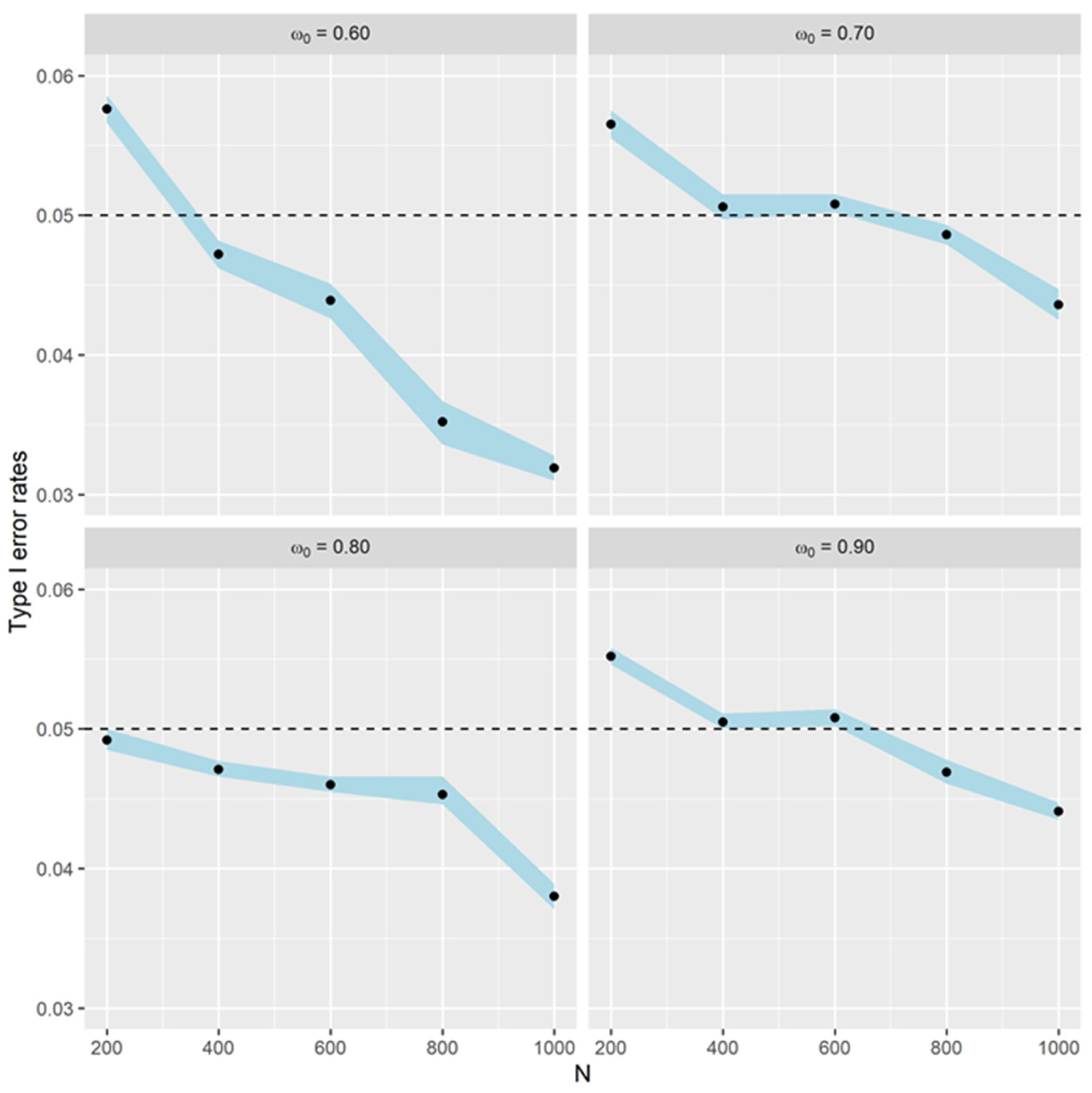
Recall that the $H_0:{\omega }_1=0$ and $H_1:{\omega }_1>0$. For this simulation study, the value of $\theta$ is fixed at $1.0$, while the value of ${\omega }_0$ varies: ${\omega }_0=0.6,0.7,0.8,0.9$. These different values of ${\omega }_0$ were selected based on previous studies [8] for the $ZOIPL$ distribution. These ${\omega }_0$s are used to study the type I error rates. The results of the simulation studies are shown in Figure 1. Figure 1 shows the type I error rate plots for varying ${\omega }_0$. When ${\omega }_0=0.60$, a sample size of 400 is sufficient to make the type I error rate fall below 0.05. On the other hand, when ${\omega }_0=0.70,0.90$, at least a sample size of 800 is needed to make a type I error rate fall below 0.05. Surprisingly, when ${\omega }_0=0.80$, even 200 samples are sufficient. It can be observed that for each value of ${\omega }_0$, the type I error rates decrease with increasing sample size $n$ and fall below $0.05$. Zhang et al. [10] mentioned that the smaller the type I error rate, the better the performance of the likelihood ratio test in controlling the error rates.

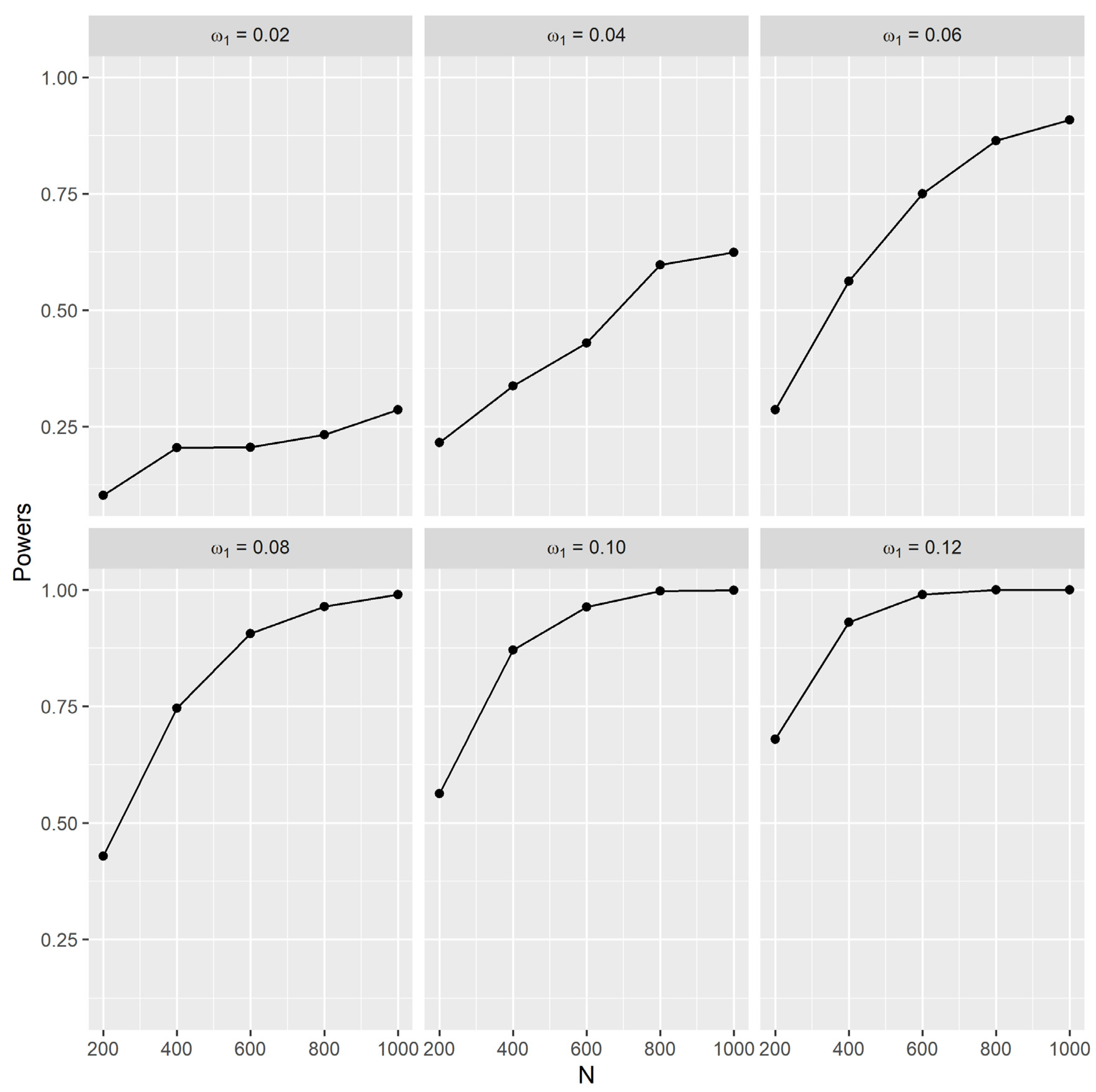
To assess the power of the test, the values of ${\omega }_1$ under $H_1$ are set at $0.02,0.04,0.06,0.08,0.10,0.12$ with $\theta =1.0$. Let $r$ be the number of rejections of $H_0$. The power of the test is obtained by calculating $r/M$ when ${\omega }_1>0$. The results of the simulation studies are shown in Figure 2. Figure 2 shows the plots for the power of the test when ${\omega }_1$ varies. It can be observed that the power of the test increases when ${\omega }_1$ and the sample size $n$ increase. Achieving at least 80% power can be carried out for ${\omega }_1\ge 0.06$ with at least a sample size of 800. For ${\omega }_1<0.06$, a large sample size is required for the test to obtain 80% power. This means that when ${\omega }_1$ is small and close to zero, the test cannot accurately identify the existence of excess ones in the data. Generally, the larger the value of ${\omega }_1$, the quicker the power of the test increases as the sample size increases.

6.4. Fixed $\theta ={\theta }_0$

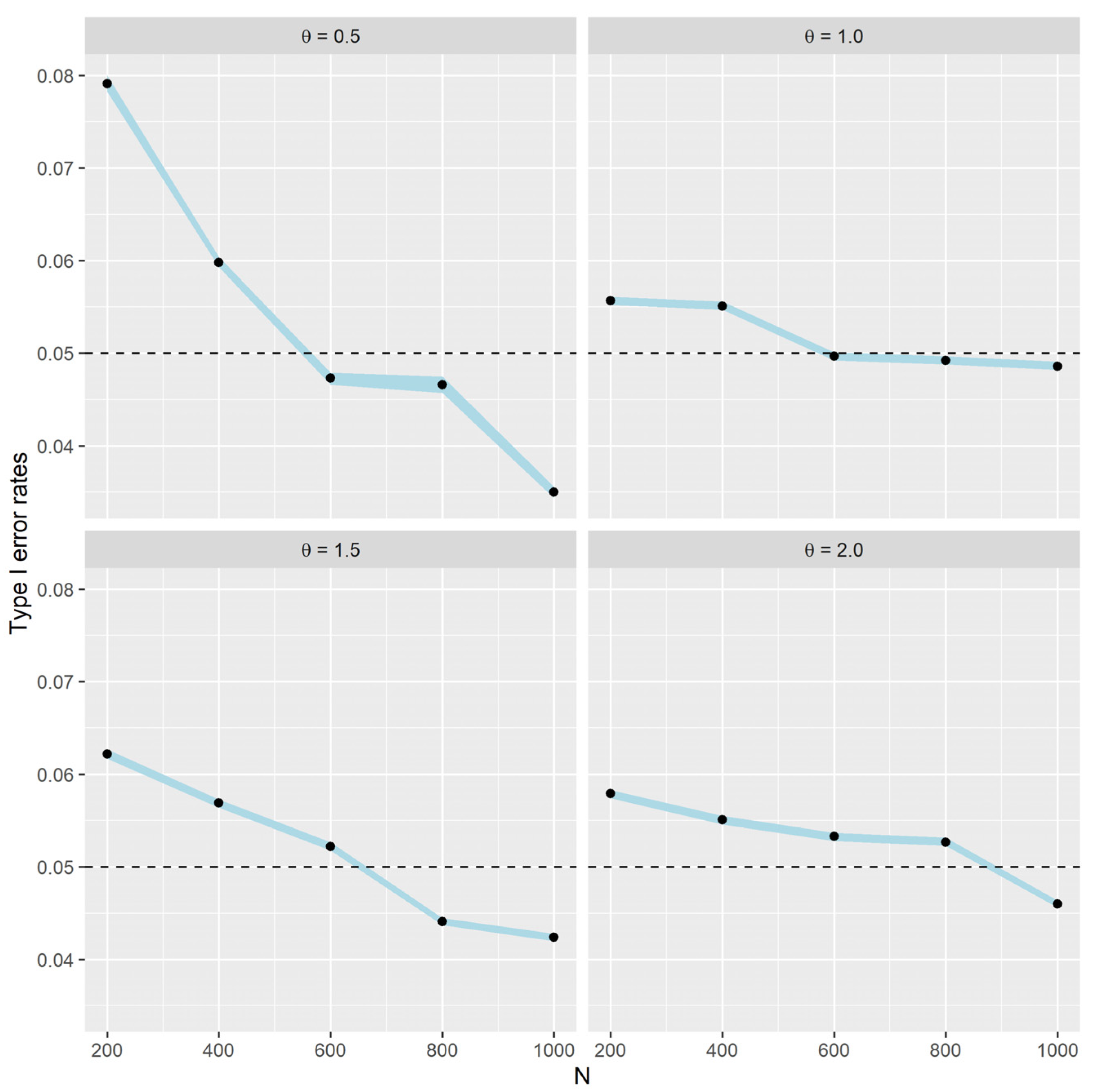
Recall that the $H_0:\theta ={\theta }_0$ and $H_1:\theta \ne {\theta }_0$. For this simulation study, the value of ${\theta }_0$ varies: ${\theta }_0=0.5,1.0,1.5,2.0$ for the study of Type I error rates. The values for ${\omega }_0=0.75$ and ${\omega }_1=0.10$ are fixed. Figure 3 shows the simulation results of the test. From Figure 3, when $\theta =0.5,1.0$, a sample size of 600 is sufficient to make a type I error rate fall below 0.05. When $\theta =1.5$, at least a sample size of 800 is needed to make a type I error rate fall below 0.05. Furthermore, a total of 1000 samples are required when $\theta =2.0$. Generally, the larger the value of $\theta$, the larger the sample size required so that the type I error becomes smaller than 0.05.

To investigate the power of the test, data are generated assuming that $\theta =1.5,2.0,2.5,3.0$, and let ${\theta }_0=1.0$. Figure 4 shows the simulation results of the test. From Figure 4, it can be noted that as the sample size increases, the power of the test increases. The further the distance between the assumed ${\theta }_0=1.0$ from the true $\theta$, the more powerful the test becomes. To achieve 80% power with 1000 samples, the true $\theta$ must be at least equal to 3.0 when ${\theta }_0=1.0$.

7. Conclusions

In this paper, various stochastic representations for the zero–one-inflated Poisson Lindley distribution have been studied extensively. The stochastic representations allow for us to view the zero–one-inflated Poisson Lindley distribution in different ways by combining several established distributions such as multinomial, degenerate, Poisson Lindley and other distributions. When handling data with excess zeroes and ones, as well as dispersion, these stochastic representations can be exploited. For example, if we are interested in studying positive count data distributions (observed) but we are presented with a full set of data containing both observed and unobserved values, instead of separating the full set of data into both observed and unobserved values, which may incur unnecessary costs, one may use the full set of data and use the fourth stochastic representation to identify the estimated parameter which describes the distribution of the unobserved data.

Besides that, some hypothesis tests have been conducted to investigate the presence of one-inflation in addition to fixed-rate parameters. The extensive simulation studies conducted investigate the ability of the test to handle both type I error and type II error rates in terms of errors as well as powers. All tests, which involve likelihood ratios, are found to be able to handle type I error rates and are found to be powerful as the sample sizes increases; hence, are found to be useful. It is suggested that a sample size of at least 1000 is sufficient for the tests to be useful.

References

1. Iddi, S.; Doku-Amponsah, K. Statistical Model for Overdispersed Count Outcome with Many Zeros: An Approach for Marginal Inference. S. Afr. Stat. J. 2016, 50, 313–337. [Google Scholar] [CrossRef]
2. Lambert, D. Zero-Inflated Poisson Regression, with an Application to Defects in Manufacturing. Technometrics 1992, 34, 1–14. [Google Scholar] [CrossRef]
3. Neelon, B.H.; O’Malley, A.J.; Normand, S.-L.T. A Bayesian Model for Repeated Measures Zero-Inflated Count Data with Application to Outpatient Psychiatric Service Use. Stat. Model. 2010, 10, 421–439. [Google Scholar] [CrossRef] [PubMed]
4. Ridout, M.; Demétrio, C.G.B.; Hinde, J. Models for Count Data with Many Zeros. In Proceedings of the XIXth International Biometric Conference, Cape Town, South Africa, 14–18 December 1998; International Biometric Society Invited Papers: Cape Town, South Africa, 1998; Volume 19, pp. 179–192. [Google Scholar]
5. Young, D.S.; Roemmele, E.S.; Yeh, P. Zero-inflated Modeling Part I: Traditional Zero-inflated Count Regression Models, Their Applications, and Computational Tools. Wiley Interdiscip. Rev. Comput. Stat. 2020, 14, e1541. [Google Scholar] [CrossRef]
6. Lin, T.H.; Tsai, M. Modeling Health Survey Data with Excessive Zero and K Responses. Stat. Med. 2012, 32, 1572–1583. [Google Scholar] [CrossRef] [PubMed]
7. Jornsatian, C.; Bodhisuwan, W. Zero-One Inflated Negative Binomial—Beta Exponential Distribution for Count Data with Many Zeros and Ones. Commun. Stat.-Theory Methods 2022, 51, 8517–8531. [Google Scholar] [CrossRef]
8. Tajuddin, R.R.M.; Ismail, N.; Ibrahim, K.; Bakar, S.A.A. A New Zero–One-Inflated Poisson–Lindley Distribution for Modelling Overdispersed Count Data. Bull. Malays. Math. Sci. Soc. 2022, 45, 21–35. [Google Scholar] [CrossRef]
9. Melkersson, M.; Olsson, C. Is Visiting the Dentist a Good Habit?: Analyzing Count Data with Excess Zeros and Excess Ones; University of Umeå: Umeå, Sweden, 1999. [Google Scholar]
10. Zhang, C.; Tian, G.L.; Ng, K.W. Properties of the Zero-and-One Inflated Poisson Distribution and Likelihood-Based Inference Methods. Stat. Interface 2016, 9, 11–32. [Google Scholar] [CrossRef]
11. Sankaran, M. 275. Note: The Discrete Poisson-Lindley Distribution. Biometrics 1970, 26, 145–149. [Google Scholar] [CrossRef]
12. Ghitany, M.E.; Al-Mutairi, D.K. Estimation Methods for the Discrete Poisson–Lindley Distribution. J. Stat. Comput. Simul. 2009, 79, 1–9. [Google Scholar] [CrossRef]
13. Tajuddin, R.R.M.; Ismail, N.; Ibrahim, K. Estimating Population Size of Criminals: A New Horvitz–Thompson Estimator under One-Inflated Positive Poisson–Lindley Model. Crime Delinq. 2022, 68, 1004–1034. [Google Scholar] [CrossRef]
14. Borah, M.; Nath, A.D. A Study on the Inflated Poisson Lindley Distribution. J. Indian Soc. Agric. Stat. 2001, 54, 317–323. [Google Scholar]
15. Joe, H.; Zhu, R. Generalized Poisson Distribution: The Property of Mixture of Poisson and Comparison with Negative Binomial Distribution. Biom. J. 2005, 47, 219–229. [Google Scholar] [CrossRef] [PubMed]
16. Self, S.G.; Liang, K.-Y. Asymptotic Properties of Maximum Likelihood Estimators and Likelihood Ratio Tests under Nonstandard Conditions. J. Am. Stat. Assoc. 1987, 82, 605–610. [Google Scholar] [CrossRef]
17. Agresti, A.; Coull, B.A. Approximate Is Better than “Exact” for Interval Estimation of Binomial Proportions. Am. Stat. 1998, 52, 119–126. [Google Scholar] [CrossRef]
18. Bradley, J.V. Robustness? Br. J. Math. Stat. Psychol. 1978, 31, 144–152. [Google Scholar] [CrossRef]
Figure 1. Type I error rates for different values of ω 0 and N .
Mathematics 12 00778 g001
Figure 2. Power of the likelihood ratio test for different values of ω 1 and N .
Mathematics 12 00778 g002
Figure 3. Type I error rates for different values of θ and N .
Mathematics 12 00778 g003
Figure 4. Power of the likelihood ratio test for different values of θ and N .
Mathematics 12 00778 g004