Long-Run Equilibrium in the Market of Mobile Services in the USA

Abstract

We develop an empirical model of the market for mobile services in the USA based on providers’ response functions. Guided by a duopoly model, we obtain our empirical response functions from an approximation of quarterly response data on smartphone subscriptions by sigmoid functions of time. The robustness analysis suggests that our model fits the data well and outperforms the regression model. Further, we demonstrate that our empirical response functions satisfy the conditions for semi-cyclic contractions which guarantee the existence, uniqueness and stability of long-run equilibrium.

1. Introduction

Using response functions in a duopoly market model, we develop an empirical model of the market for mobile services in the USA. The wireless telecommunications market is dominated by two providers, AT&T and Verizon, which serve over $75\%$ of the market. Our empirical strategy relies on the approximation of quarterly data on smartphone subscriptions by continuous functions from the sigmoid family. Guided by our duopoly model, we reformulate this approximation to obtain providers’ response functions. Our model is parsimonious and outperforms the alternative approach of directly estimating the response functions with a polynomial specification. Importantly, our model features unique equilibrium because the empirical response functions satisfy the conditions for semi-cyclic contractions obtained in [1]. In fact, numerical simulations in the appendix suggest that the model converges to equilibrium from a range of initial conditions significantly wider than their hypotheses.

Market models relying on response functions date as early as [2], which introduces a model of a market where a few players (known as an oligopoly market) control the price and supply quantity of the goods being traded. In the original model, a few players sequentially respond to each others’ quantities in a rational way, i.e., pursuing profit maximization in their response. The subsequent literature has enriched the response function approach to model market equilibrium by avoiding the rationality assumption [3,4]. In another enrichment of the approach by [5], each company attempts to guess what change in production the other players will make in time t, while still using data up to period t.

In a baseline Cournot duopoly model, two producers (firms) are competing for the same consumers and striving to meet the demand with overall production of $X=x_1+x_2$, where $x_i$, $i=1,2$, is the amount produced by the $i^{th}$ firm. The market price is given by $P\left(X\right)=P(x_1+x_2)$, which is the inverse of the demand function. The (inverse) demand does not change over time and the producers cannot alter it. Their production technologies are reflected in their cost functions $c_i\left(x_i\right)$. Both firms act rationally, i.e., each firm chooses quantity $x_i$ to maximize its profit, with profit (payoff) functions:

$${\mathsf{\Pi }}_i(x_1,x_2)=x_{i}P(x_1+x_2)-c_i\left(x_i\right),i=1,2.$$

(1)

Notably, each firm $i=1,2$ takes its competitor’s decision as given, formally solving $\max \{{\mathsf{\Pi }}_i(x_i,x_i):x_i,\mathrm{assuming} \mathrm{that}{x}_j,j\ne i\mathrm{is} \mathrm{fixed}\}$. Provided that functions P and $c_i$, $i=1,2$, are differentiable, firms’ optimal solutions satisfy the system of equations:

$$\left|\begin{array}{c}\frac{\partial {\mathsf{\Pi }}_1(x_1,x_2)}{\partial x_1}=P(x_1+x_2)+x_1{P}^{\prime }(x_1+x_2)-c_1^{\prime }\left(x_1\right)=0\hfill \\ \frac{\partial {\mathsf{\Pi }}_2(x_1,x_2)}{\partial x_2}=P(x_1+x_2)+x_1{P}^{\prime }(x_1+x_2)-c_2^{\prime }\left(x_2\right)=0.\hfill \end{array}\right.$$

(2)

There are various ways to approach (2). The direct approach of obtaining $x_1=b_1\left(x_2\right)$ and $x_2=b_2\left(x_1\right)$, called response functions [6], may encounter technical limitations. Specifically, exact response functions $b_i\left(x_j\right)$ and their fixed points $b_i\left(y_j\right)=y_i,i\ne j,i,j=1,2$, may be difficult or impossible to obtain. Further, if the model is not a stable one, exact or approximate solutions may not be even close to the market equilibrium. Separately to these concerns, one needs to obtain sufficient conditions for a solution $(y_1,y_2)$ of (2) to be a solution of (1) which are either the second-order conditions, i.e., $\frac{{\partial }^2{\mathsf{\Pi }}_i(x_1,x_2)}{\partial x_i^2}(y_1,y_2)<0$ for $i=1,2$, or payoff functions ${\mathsf{\Pi }}_i$ being concave ones [7,8,9]. Finally, this approach assumes that the payoff functions ${\mathsf{\Pi }}_i$ are differentiable, while in certain settings these may not even be continuous and require different optimization techniques.

In a departure from the direct approach focused on obtaining solutions $x_1=b_1\left(x_2\right)$ and $x_2=b_2\left(x_1\right)$ to (2), ref. [10] considers the alternative response functions:

$$x_i=\frac{c_i^{\prime }\left(x_i\right)-P(x_1+x_2)}{P^{\prime }(x_1+x_2)}=F_i(x_1,x_2),i=1,2.$$

The authors analyze these functions in the context of modeling firms’ responses over time.

We follow this departure from the direct approach of solving maximization (1). Our main premise is that each firm responds to their and that of their competitor’s past period market results (decisions), i.e., for each ordered pair $(x_1,x_2)$, where $x_1$ is the quantity sold by the first firm and $x_2$ is the quantity sold by the second firm, they change their output accordingly. There are two functions $F_1(x_1,x_2)$ and $F_2(x_1,x_2)$, which are their responses to the ordered pair of the quantities sold $(x_1,x_2)$. Importantly, turning to firms’ response functions substitutes the maximization problem of (1) with a coupled fixed point problem. This, in turn, renders all assumptions of concavity, differentiability or even continuity unnecessary [1,10]. In particular, ref. [1] shows that in the settings of [11] it is possible to widen their conditions for ensuring the existence and uniqueness of the market equilibrium beyond the settings of payoff function maximization.

An extensive study on the oligopoly markets can be found in [7,8,9,12]. Some recent results on oligopoly markets are in [13,14,15,16,17] and those of duopoly markets especially are in [18,19,20]. The approach for the investigation of equilibrium in duopoly markets by response functions was introduced in [10] and further investigated in [1].

In this paper, we use response functions in a duopoly market to build an empirical model of the USA wireless telecommunications market. We horse race two alternative approaches of obtaining the response functions: a direct approach of fitting polynomial specification with the proposed more conceptually coherent approach combining a time series approximation of the market quantities with a theory of market response in a duopolistic market. This paper concludes with evidence on the statistical superiority of the proposed approach and on the range of starting values guaranteeing convergence to unique long-run equilibrium.

2. Materials and Methods

2.1. Coupled Fixed Points of Semi-Cyclic Maps

Let A be a nonempty subset of a metric space $(X,\rho )$. The map $T:A\to A$ is said to have a fixed point $x\in A$ if $\rho (\xi ,T\xi )=0$ [21].

Following [21], there is an enormous number of generalizations. We will use the idea of a coupled fixed point introduced in [22].

Definition 1 

([22,23]). Let A be a nonempty subset of a metric space $(X,\rho )$, $F:A\times A\to A$. An ordered pair $(x,y)\in A\times A$ is said to be a coupled fixed point of F in A if $x=F(x,y)$ and $y=F(y,x)$.

A deep result on the connection between fixed points and coupled fixed points is obtained in [24]. It is proven there that we can consider instead of the map $F:A\times A\to A$ the map $T:A\times A\to A\times A$, defined by $T(x,y)=\left(F\right(x,y),F(y,x\left)\right)$. Then, the ordered pair $(x,y)$ is a coupled fixed point for F if and only if it is a fixed point for T.

The idea to investigate for the existence and uniqueness of fixed points cyclic maps, i.e., $T:A\to B$ and $T:B\to A$, instead of self maps was initiated in [25]. This was further generalized in the context of maps of two variables in [26].

Definition 2 

([26]). Let A and B be nonempty subsets of a metric space $(X,\rho )$. The ordered pair of maps $(F,G)$, $F:A\times A\to B$ and $G:B\times B\to A$ is called a cyclic ordered pair of maps.

Definition 3 

([26]). Let A and B be nonempty subsets of a metric space $(X,\rho )$ and $(F,G)$ be a cyclic ordered pair of maps. An ordered pair $(x,y)\in A\times A$ is said to be a coupled fixed point of F in A if $x=F(x,y)$ and $y=F(y,x)$.

Definition 4 

([26], Definition 3.4 and Theorem 4.1). Let A and B be nonempty subsets of a metric space $(X,\rho )$ and $(F,G)$ be a cyclic ordered pair of maps. We say that the cyclic ordered pair of maps $(F,G)$ is a cyclic contraction if there exists $\alpha \in (0,1/2)$ such that

$$\rho \left(F\right(x,y),G(u,v\left)\right)\le \alpha \left(\rho \right(x,u)+\rho (y,v\left)\right)$$

holds for every $x,y\in A$ and $u,v\in B$.

Theorem 1 

([26], Theorem 4.1). Let A and B be nonempty subsets of a metric space $(X,\rho )$ and $(F,G)$ be a cyclic contraction. Then, F and G have a unique common coupled fixed point $(x_0,y_0)\in A\times A\cup B\times B$, i.e., $x_0=F(x_0,y_0)=G(x_0,y_0)$ and $y_0=F(y_0,x_0)=G(y_0,x_0)$.

Moreover, it is proven in [27] that $x_0=y_0$.

In order to apply the technique of coupled fixed points and a generalization of coupled fixed points, the above-mentioned notion was presented in [10]. When we investigate duopoly with players’ response functions F and G, we see that each player, using the information about their production and the rival’s production, chooses a change in their production, i.e., $F:A\times B\to A$, $G:A\times B\to B$. Thus, we reach maps that are not the cyclic type of maps from Definition 2. The authors of [10] called these new type of maps cyclic again. A more natural name is introduced in [28], where the authors called them an ordered pair of semi-cyclic maps.

Definition 5 

([10,28]). Let A, B be nonempty subsets of a metric space $(X,\rho )$ and $F:A\times B\to A$, $G:A\times B\to B$. An ordered pair $(F,G)$ is called an ordered pair of semi-cyclic maps.

Definition 6 

([10,28]). Let A, B be nonempty subsets of a metric space $(X,\rho )$ and $(F,G)$ be an ordered pair of semi-cyclic maps. An ordered pair $(\xi ,\eta )\in A\times B$ is called a coupled fixed point of $(F,G)$ if $\xi =F(\xi ,\eta )$ and $\eta =G(\xi ,\eta )$.

Whenever $A=B$ and $G(x,y)=F(y,x)$, we obtain the notion of coupled fixed points from Definition 1.

There is a sequence of results that guarantees the existence and uniqueness of coupled fixed points for semi-cyclic kinds of maps and thus the existence and uniqueness of market equilibrium in duopoly markets [1,10,28].

We will use a result from [1].

Theorem 2 

(Assumption 1, [1]). Let us consider a duopoly market, satisfying the following:

1. 

The two players are producing homogeneous goods that are perfect substitutes.

2. 

The first player can produce quantities from the set A, and the second one can produce quantities from the set B, where A and B are closed, nonempty subsets of a complete metric space $(X,\rho )$.

3. 

Let there be a closed subset $D\subseteq A\times B$ and maps $F:D\to A$, $G:D\to B$ such that

$$\left(F\right(x,y),G(x,y\left)\right)\subseteq D$$

for every $(x,y)\in D$ are the response functions for players one and two, respectively.

4. 

Let $\alpha <1$, such that the inequality:

$$\rho \left(F\right(x,y),F(u,v\left)\right)+\rho \left(G\right(x,y),G(u,v\left)\right)\le \alpha \left(\rho \right(x,u)+\rho (y,v\left)\right)$$

(3)

holds for all $(x,y),(u,v)\in A\times B$.

Then, there is a unique market equilibrium pair $(\xi ,\eta )$ in D, i.e., $\xi =F(\xi ,\eta )$ and $\eta =G(\xi ,\eta )$.

If in addition the symmetry condition $G(x,y)=F(y,x)$ holds, then the market equilibrium pair $(\xi ,\eta )$ satisfies $\xi =\eta$.

For any initial start of the market $(x_0,y_0)$, we will consider the sequence of iterated productions of the two players $(x_n,y_n)$, defined by $(x_n,y_n)=(F(x_{n-1},y_{n-1}),G(x_{n-1},y_{n-1}))$. It leads to a more complicated iterated formula,

$$x_1=F(x_0,y_0),y_1=G(x_0,y_0),$$

$$x_2=F(F(x_0,y_0),G(x_0,y_0)),y_2=G(F(x_0,y_0),G(x_0,y_0)),$$

$$x_3=F(F(F(x_0,y_0),G(x_0,y_0)),G(F(x_0,y_0),G(x_0,y_0))),$$

$$y_3=G(F(F(x_0,y_0),y_1),G(F(x_0,y_0),G(x_0,y_0))),$$

etc. We will sometimes use the notation $x_n=F^n(x_0,y_0)=F^{n-1}(x_{n-1},y_{n-1})$, $y_n=G^{n-1}$$(x_{n-1},y_{n-1})$.

A similar result to that in Theorem 2 is obtained in [10], where condition (3) is replaced by the inequality

$$\rho \left(F\right(x,y),F(u,v\left)\right)+\rho \left(f\right(z,w),f(t,s\left)\right)\le \alpha \rho (x,u)+\beta \rho (y,v)+\gamma \rho (z,t)+\delta \rho (w,s)$$

(4)

for all $(x,y),(u,v),(z,w),(t,s)\in A\times B$ (Assumption 1, [10]).

It is proven in [1] that both conditions are equivalent.

2.2. Approximation with Sigmoid Functions

Our approach to work with sigmoid functions is motivated by a fundamental result for approximating continuous functions due to [29]. The author demonstrates that for every continuous function in a closed interval, there exists a finite linear combination of sigmoids that approximates the function with a predetermined accuracy. (Actually, this follows from Stone’s Theorem, which states that every Stone algebra is dense in the space of continuous functions over a compact set. Note that linear combinations of the sigmoids together with constants are trivially such a Stone algebra.) In the following years, the theory of approximating real data with the sigmoids has seen rapid development, e.g., see [30,31,32,33,34].

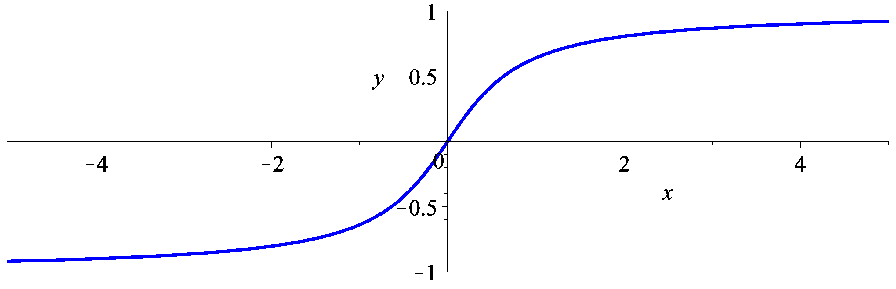
A sigmoid function (also known as an S-curve) is an increasing function of two horizontal asymptotes $y=a$ and $y=b$ (Figure 1).

Then, approximations of real-world data are sought through a linear combination of a set of sigmoidal curves. Importantly, there is a trade off between the accuracy of the fit and parsimony. To pick a representation, it is common to gauge models’ performance by testing a hypothesis of matching real data with the approximations, e.g., see [30,31,32,33,34].

Sigmoid functions have gained popularity with applications ranging from artificial neural networks (as activation functions) to simple classification algorithms. In our model, we use sigmoid functions to better capture the following important characteristics of our settings:

• Nonlinearity in an intuitive way with respect to a small number of parameters.
• Switching agents’ behavior, e.g., between different suppliers, products, etc.
• As a robust technical tool capable of modeling changes in a modular way by scaling these changes down to a predefined range (a to b), thus allowing us to incorporate strategies that are built on incremental changes of output.

In general, one of the main advantages for relying on approximations with sigmoid functions is that these can be applied to both continuous and binary variables (in the latter case, approximation with sigmoids involves the introduction of a threshold).

Related to the trade off above, there are infinitely many continuous curves passing through the data points. Thus, a starting point is the choice of curves of a certain class, i.e., meeting predetermined conditions. For example, consider the class of the logistic curve $f\left(x\right)=\frac{1}{1+e^{-x}}$, which is a solution to the logistic differential equation

$$\frac{dS}{dx}=c(S-a)(b-S),$$

(5)

for $c=b=1$ and $a=0$. Once a class of curves is decided on, the approximation proceeds with some kind of minimization of the deviation between the real and the approximated data by some criterion (e.g., the method of least squares). (Such approximations can be made using modern computer algebra systems. For example, in Wolfram Mathematica, this can be calculated with the “Fit command”).

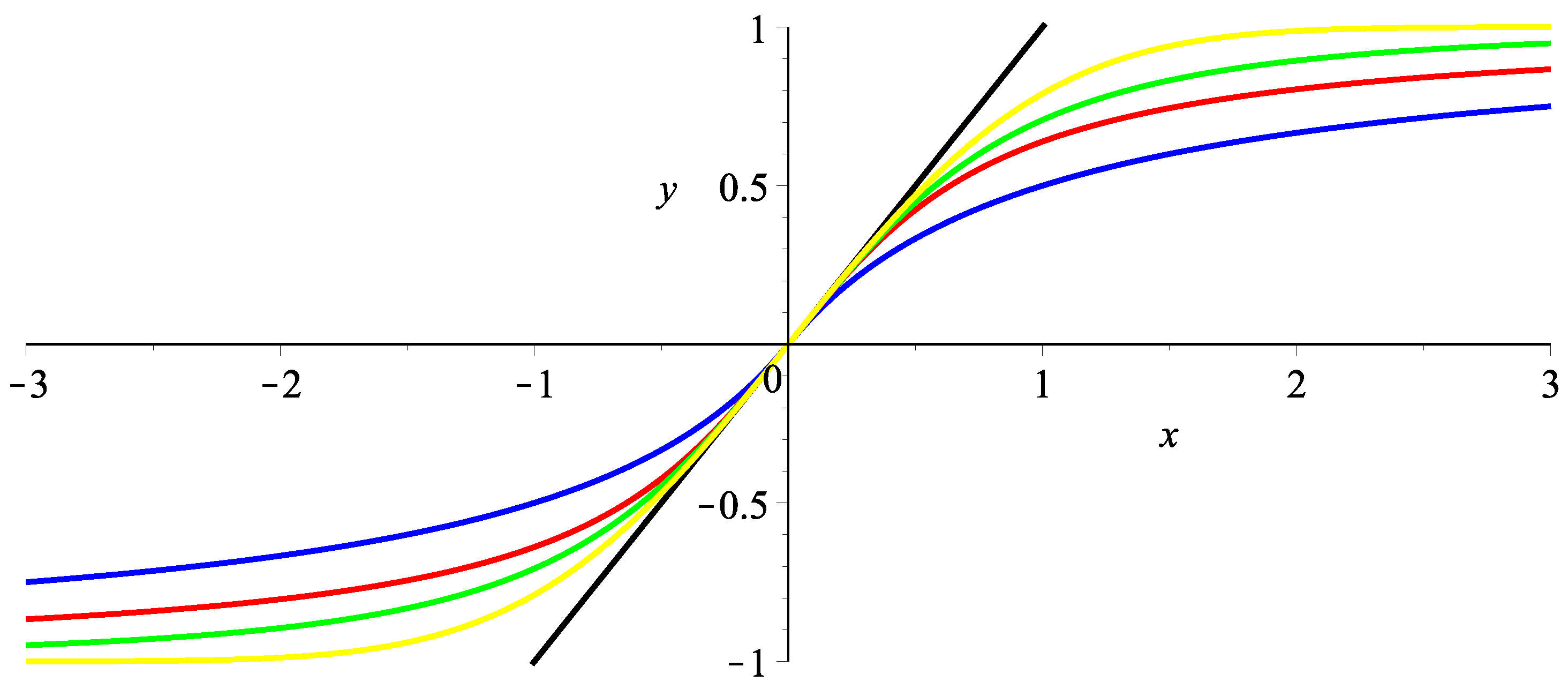
The main classes of sigmoids are presented in Figure 2. They have similar behavior but differ on the intervals that double the population. These functions are normed so that the derivative at zero equals 1.

The choice of a particular type of sigmoid is determined by the assumption about the type of impact, e.g., the rate of change, may depend on both the current state and the constraints on the sigmoid ($a\le S\left(x\right)\le b$). The simplest type of such dependence is described by the logistic Equation (5). Its solution is the logistic curve

$$S\left(x\right)=a+\frac{b-a}{1+e^{-c(x-x_0)}},$$

(6)

where $x_0$ is the “inflection point” of the curve. A generalization of the logistic equation giving a more general form of sigmoid is

$$\frac{dS}{dx}=cg(S-a)h(b-S),$$

where g and h are non-decreasing functions. A particular example is the equation

$$\frac{dS}{dx}=c{(S-a)}^{\alpha }{(b-S)}^{\beta },\alpha ,\beta >0.$$

Sigmoids describe evolutionary processes very well because those are characterized by three stages: slow growth, until reaching a critical region of rapid growth, followed by slow growth. Further, the population size is bounded from above. Indeed, the S-curves describe such processes well. Following [35], knowing how long it takes for the population to double suffices for constructing the sigmoid that describes the evolutionary process continuously. This approach is remarkable for the fact that from information about a small interval of time, we can reconstruct the evolutionary behavior over the entire interval.

The model we are looking at is the number of mobile users in the USA. It is well known that this market starts from zero users and its growth is limited (it is possible for one person to use more than one service, not too many in number). This means that sigmoids will describe this process well. We consider linear combinations of sigmoids to obtain a better approximation.

2.3. Testing Model’s Fit

Naturally, there are differences between our continuous model and the discrete real-world data. We interpret these differences as insignificant random deviations. To gauge our model’s performance and the insignificance of these deviations, it is common to perform statistical testing. We use Pearson ${\chi }^2$ and the Kolmogorov–Smirnov test. These two tests are most commonly applied in testing non-parametric hypotheses (testing whether a sample has a predetermined distribution or whether two samples have the same distribution).

The Pearson ${\chi }^2$ test is an asymptotic one based on the Central Limit Theorem. The test statistic has a distribution that is not actually known but converges asymptotically (very fast, provided that the hypothesis is true) to a Pearson ${\chi }^2$ distribution. The Kolmogorov–Smirnov test is more reliable, but more complicated to apply. It is based on a Kolmogorov result for the supremum of the difference between the assumed distribution and the empirical sampling distribution under the “null hypothesis”.

By these tests, we check whether the differences between the empirical and approximated data are insignificant random deviations (acceptance of the null hypothesis) or significant (rejection of the null hypothesis). Wolfram Mathematica calculates the probability of randomness of deviations (p-value). We seek significance with p-value < 0.05 (the $5\%$ limit).

3. Empirical Response Functions

We have data for the number of smartphone subscribers to two companies over a ten-year period, ${\left\{(x_n,y_n)\right\}}_{n=0}^{40}$. Formally, $(x_n,y_n)\in X\times Y$, where X and Y are the sets of possible numbers of consumers for each firm. We are searching for an ordered pair of semi-cyclic maps $(F,G):X\times Y\to X\times Y$ that satisfies the equality $(F(x_n,y_n),G(x_n,y_n))=(x_{n+1},y_{n+1})$, i.e., the response function of each company.

3.1. Data and Empirical Strategy

We use publicly available information on the distribution of mobile operators in the USA for the period 2009–2021, distributed by quarters in percentage of market share from https://www.statista.com (accessed on 20 March 2022).

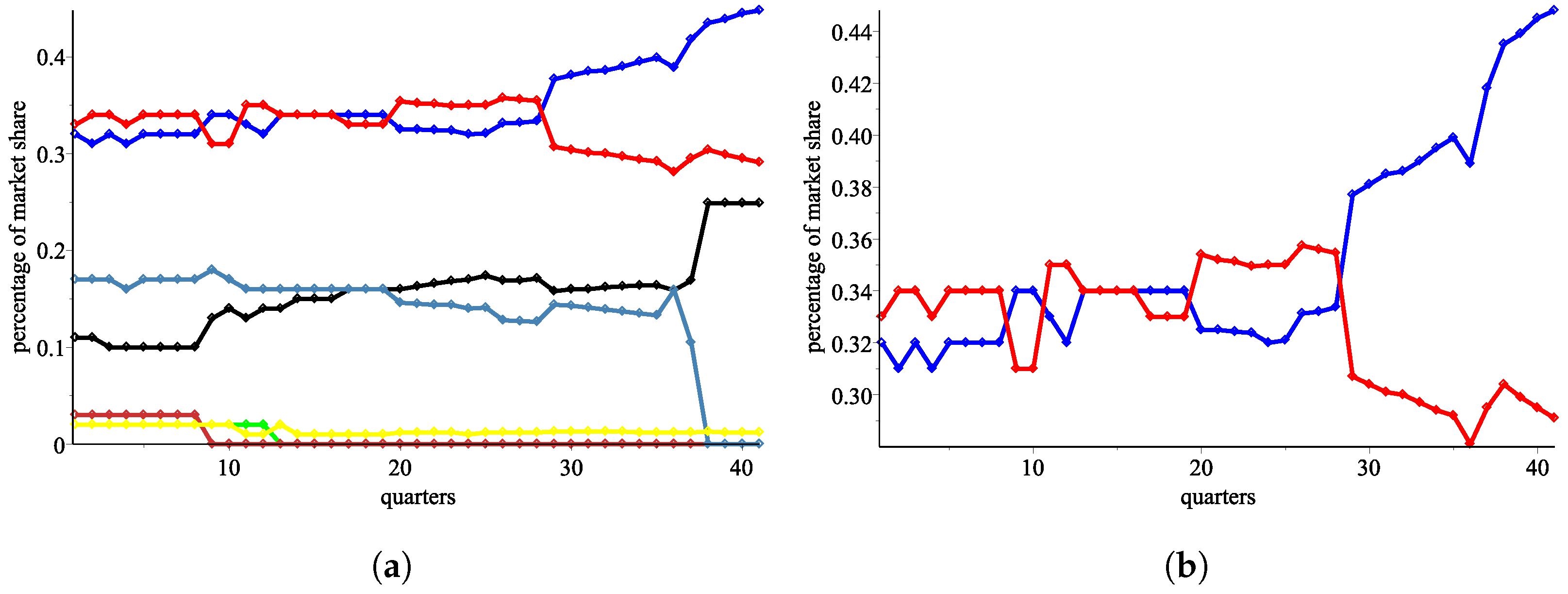
In Figure 3a, we plot the data in a graphic view.

Our analysis proceeds with the two biggest mobile service providers, AT&T (in blue color) and Verizon (in red color). Specifically, we abstract from all smaller providers, assuming that the two big operators AT&T and Verizon respond only to each other and not to the rest of the market. While we acknowledge that a third operator has a growing share, it is only in the last four quarters, and handling a market with three participants with the proposed methods remains an open question. The lack of long-term data for the third operator and the complexity of modeling motivates us to analyze the market as a duopoly.

We plot in Figure 3 the percentage shares only for the two biggest mobile providers. We try to model the response functions of the two big providers ($AT\&T$ and $Verizon$) in the form of semi-cyclic maps $F:X\times Y\to X$ and $G:X\times Y\to Y$, where X and Y are the sets of consumers for $AT\&T$ and $Verizon$, respectively, rather than the percentage shares in the market. (Formallyspeaking, there is a structural change in the market taking place sometime in the 36th quarter, where something happens and the other big player ($Sprint$) disappears and its customers are reallocated. Again, handling this structural break is challenging both from the point of insufficient data and from a technical viewpoint. Furthermore, according to data from www.statista.com (accessed on 15 February 2024) for the third quarter of 2023, AT&T has $46\%$ and Verizon has $28\%$, totaling $74\%$, from a market of around 310 million mobile subscribers. With this concentration, we believe that the duopoly model provides a reasonably good description of the market and a probable equilibrium that would last if no changes had occurred, such as new regulations or the entry or exit of operators from the market.)

3.2. Approximation of the Evolution of Smartphone Subscriptions over Time

We need to address a few challenges before we proceed with the construction of empirical response functions.

The real data at our disposal are discrete. We have information at a finite number of moments in time, but we will try to construct continuous response functions. It is well known that an infinite number of functions pass through a finite number of points even when the form of these functions is known to some extent—for example, continuous, differentiable, etc. We will assume that the response functions will be differentiable and that their partial derivatives will be bounded so that no too-big changes of their market shares can appear. In addition, the data are not always accurate enough in practice, i.e., values are known to have some error.

We are searching an approximation of the discrete data of the total number of users of mobile services in the USA by a function S. Note the assumption that S is bounded ($0\le a\le S\left(x\right)\le b$), where b is the upper bound in millions for the possible number of mobile users in the USA, naturally limited. Therefore, a sigmoid kind of function will best fit the data [29,36]. The sigmoid functions are monotone and nonlinear, with an S-type graph and with derivatives that have a bell-formed graph and a pair of horizontal asymptotes.

The choice of the specific type of sigmoid [29,36] is determined by the assumption of the type of impact. For the rate of change, we assume that it depends on both the current state and the constraints on the sigmoid $0\le a\le S\left(x\right)\le b\le 334.5$. The simplest type of such dependence is described by the logistic differential Equation (5), representing a special case of the Bernoulli differential equation, where S is the unknown sigmoid function, which best fits the data, a and b are its lower and upper horizontal asymptotes and c is a coefficient of the proportionality factor, characterizing the force of impact (usually it is about 1). In our model, we set $c=1$.

The meaning of the form of this equation [29] is that for small values of the variable y, the rate of change is approximately proportional to the accumulated value y, and for values close to the maximum value of y, the rate of change will be close to 0.

The solution of this equation is the so-called logistic curve (6) [37], where $x_0$ is the starting point of the available data.

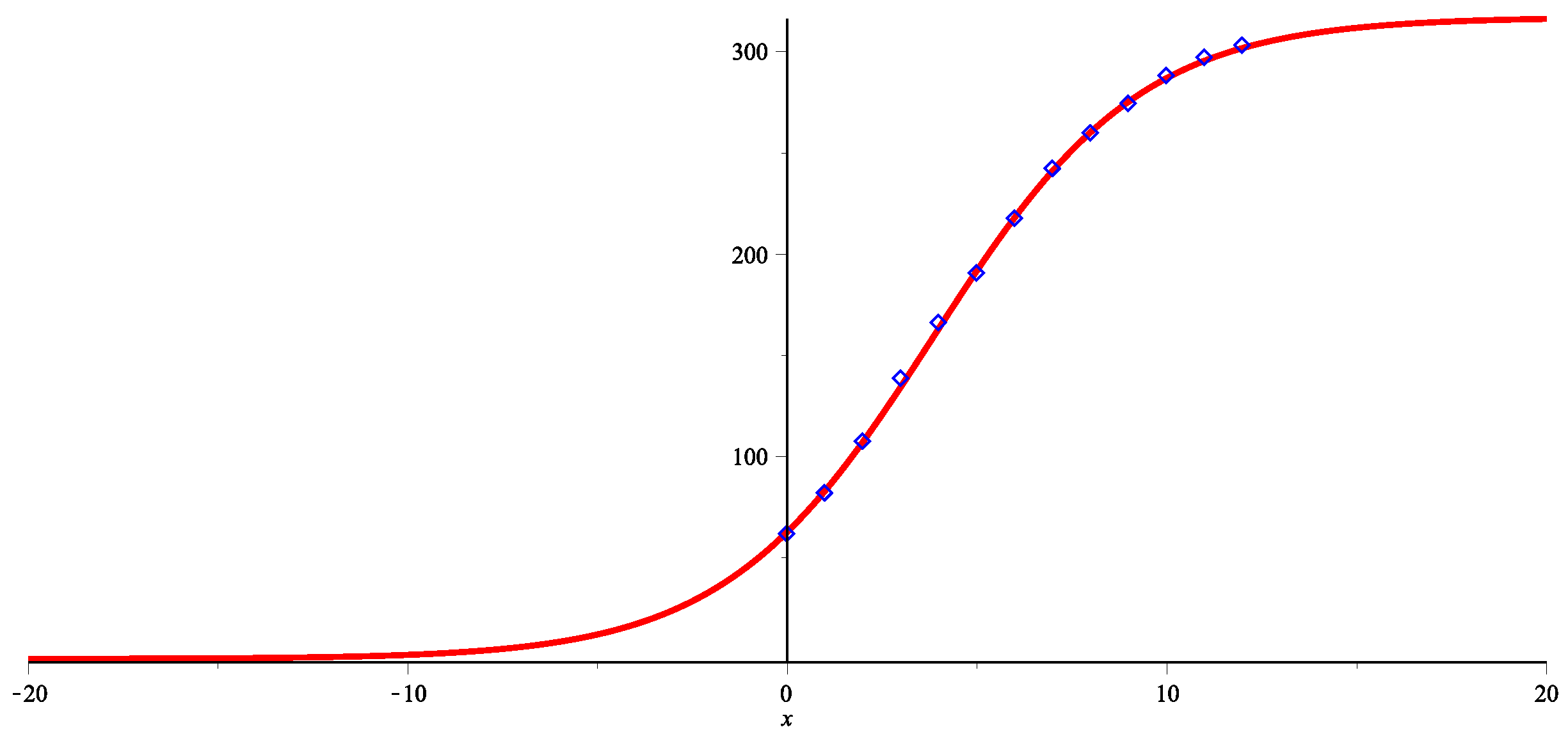
We obtain an approximation curve for the total number of mobile consumers in the USA in the form

$$S\left(y\right)=\frac{300}{0.94603451639337+3.82872969606594e^{-0.3654826455459846y}},$$

where y is number of years from the starting point $y_0=2009$ (Figure 4).

The maximum number of smartphones in the USA in the near future will not exceed $\frac{300}{0.9460}=317.125$ million smartphones, which is a realistic estimate given the actual number of smartphones at the time of the study: the number in 2021 is set to be $296.8$ million and in the nearby future the number in 2022 is set to be 302 million.

We see that the function S fits the data very well (Figure 4). We see that the start of the process is about 15 years away from the zero one (2009), which is somewhere in the year $1993/94$. It is actually close to the real beginning of mobile services. Therefore, the sigmoid function S presents a fair model of the number of mobile users, and we can assume that the total number will not exceed 320 million in the near future.

With the use of the function S, we calculate an approximation of the total number of mobile service users in quarters, rather than years.

3.3. Construction of the Response Function

We prefer to use three different notations for the ordered pairs of response functions to distinguish the three models that we derive from the available empirical data. We denote by $(F,G)$ the model constructed using least squares, by $(F_1,G_1)$ that obtained with sigmoid functions and by $(F_2,G_2)$ the linear approximation of $(F_1,G_1)$.

We will use intuition from our duopoly model to reformulate the time series approximation of the total number of consumers and obtain an approximation of the response functions. Specifically, we use the method of least squares for functions of two variables to approximate the response functions of the two biggest mobile operators in the market $F:U\times V\to U$ and $G:U\times V\to V$, where U and V are the sets of the possible numbers of consumers. We will minimize ${\sum }_{k=1}^{39}{(F(u_k,v_k)-u_{k+1})}^2$ and ${\sum }_{k=1}^{39}{(G(u_k,v_k)-v_{k+1})}^2$, where $u_i$ is the total number of consumers of AT&T and $v_i$ is that of Verizon for the quartile i. We will search the functions F and G to be a linear combination of the functions 1, u, v, $uv$, $u^2$, $v^2$, $u^{2}v$, $u{v}^2$, $u^3$ and $v^3$. Let us set $f_0(u,v)\equiv 1$, $f_1(u,v)\equiv u$, $f_2(u,v)\equiv v$, $f_3(u,v)\equiv u^2$, $f_4(u,v)\equiv uv$, $f_5(u,v)\equiv v^2$, $f_6(u,v)\equiv u^3$, $f_7(u,v)\equiv u^{2}v$, $f_8(u,v)\equiv u{v}^2$ and $f_9(u,v)\equiv v^9$. Let us denote $F(u,v)={\sum }_{i=0}^9{a}_i{f}_i(u,v)$ and $G(u,v)={\sum }_{i=0}^9{b}_i{f}_i(u,v)$. We look for ${\left\{(a_i,b_i)\right\}}_{i=0}^9$ that minimize the problems

$$\left|\begin{array}{c}{\displaystyle \min \left\{\sum _{k=1}^{39}F(u_k,v_k)-u_{k+1}\right\}}\hfill \\ {\displaystyle \min \left\{\sum _{k=1}^{39}G(u_k,v_k)-v_{k+1}\right\}.}\hfill \end{array}\right.$$

(7)

As noted above, there is an infinite number of response functions that will fit the data, so we need to make a few regularizations. We assume that the response functions have partial derivatives, which satisfy certain conditions. Intuitively, we assume that the mobile operators cannot increase or decrease their numbers of consumers too fast. Thus, we search for a solution of (7) satisfying

$$\left|\begin{array}{c}{\displaystyle \sup \left\{\left|\frac{\partial F}{\partial u}(u,v)\right|+\left|\frac{\partial G}{\partial u}(u,v)\right|:u\in [0,90],v\in [0,143]\right\}<1}\hfill \\ {\displaystyle \sup \left\{\left|\frac{\partial F}{\partial v}(u,v)\right|+\left|\frac{\partial G}{\partial v}(u,v)\right|:u\in [0,90],v\in [0,143]\right\}<1}\hfill \end{array}\right.$$

(8)

Wolfram Mathematica delivers two response functions F and G for $AT\&T$ and $Verizon$, respectively:

$$\begin{array}{ccc}G(u,v)\hfill & =\hfill & 16.3284+0.71983021v+0.04093051u\hfill \\ & & {\displaystyle +\frac{8.05785}{{10}^6}{v}^2+\frac{2.5263}{{10}^4}uv-\frac{6.44817}{{10}^6}{u}^2}\hfill \\ & & {\displaystyle +\frac{4.03746}{{10}^8}{v}^3+\frac{1.2852}{{10}^8}{v}^{2}u-\frac{5.26538}{{10}^8}v{u}^2-\frac{3.21218}{{10}^8}{u}^3}\hfill \end{array}$$

and

$$\begin{array}{ccc}F(u,v)\hfill & =\hfill & 4.15613+0.179974v+0.782994u\hfill \\ & & {\displaystyle +\frac{2.46193}{{10}^6}{v}^2+\frac{3.41712}{{10}^4}uv+\frac{7.43075}{{10}^5}{u}^2}\hfill \\ & & {\displaystyle +\frac{1.52606}{{10}^8}{v}^3+\frac{1.58968}{{10}^8}{v}^{2}u+\frac{2.16049}{{10}^7}v{u}^2+\frac{1.47514}{{10}^6}{u}^3,}\hfill \end{array}$$

where u is the total number of customers of AT&T and v is the total number of customers of Verizon.

For each ordered pair $(u,v)$, the response functions F and G present the reactions of each of the mobile operators that leads to a change in the number of their consumers, i.e., $\left(F\right(u,v),G(u,v\left)\right)$ will be the number of consumers for each of the players after reacting to the market results $(u,v)$.

3.4. Alternative Model with Consumer Shares

An alternative approach to modeling these data is in shares as opposed to levels. That is, we can work with functions representing the market share instead of the number of consumers. From the market share, we can recover the real number of subscribers using the total market consumers. As before, we approximate the data from Figure 3a as time series by sigmoid functions.

Let us denote with $S_1$ and $S_2$ the functions that represent the percentage share of the mobile providers $AT\&T$ and $Verizon$ as a function of time, respectively. Due to the assumption that f and g are percentages, it follows that they are bounded ($0\le a\le s_i\left(x\right)\le b\le 1$). This assumption leads us to search for a sigmoid function that will fit best the data, as it was performed for the approximation of the total number of mobile service users. We look for an approximation of the form of a linear combination of logistic curves $A+B{f}_i\left(t\right)+C{g}_i\left(t\right)$, $t\in {\left\{t_k\right\}}_{k=0}^p$, n and m, where $f_i\left(t\right)=\frac{1}{1+e^{-(t-n)}}$ and $g_i\left(t\right)=\frac{1}{1+e^{-(t-m)}}$. The functions f and g are of the same class of sigmoidal functions, but with different parameters. One of the functions represents the desire of one operator to increase its users, and the other function is the behavior of its competitor, which leads to a decrease in the users of the first participant. The two functions taken together give the reaction, but over time, not as a reaction to market performance.

This kind of logistic curve describes change in the market share of the operator so that their policy $f_1$ tries to increase its impact and the policy of the other player $g_1$ tries to decrease its impact. The constants A and $A+B+C$ are, respectively, the lower and upper limits (horizontal asymptote) of the described market share of the considered mobile operator.

Using a series of numerical experiments in the Wolfram Mathematica System, the coefficients A, B and C were calculated for $n=28$ and $m=36$, best describing the available quarter data on the percentage presence of the market of the two mobile operators $AT\&T$ and $Verizon$.

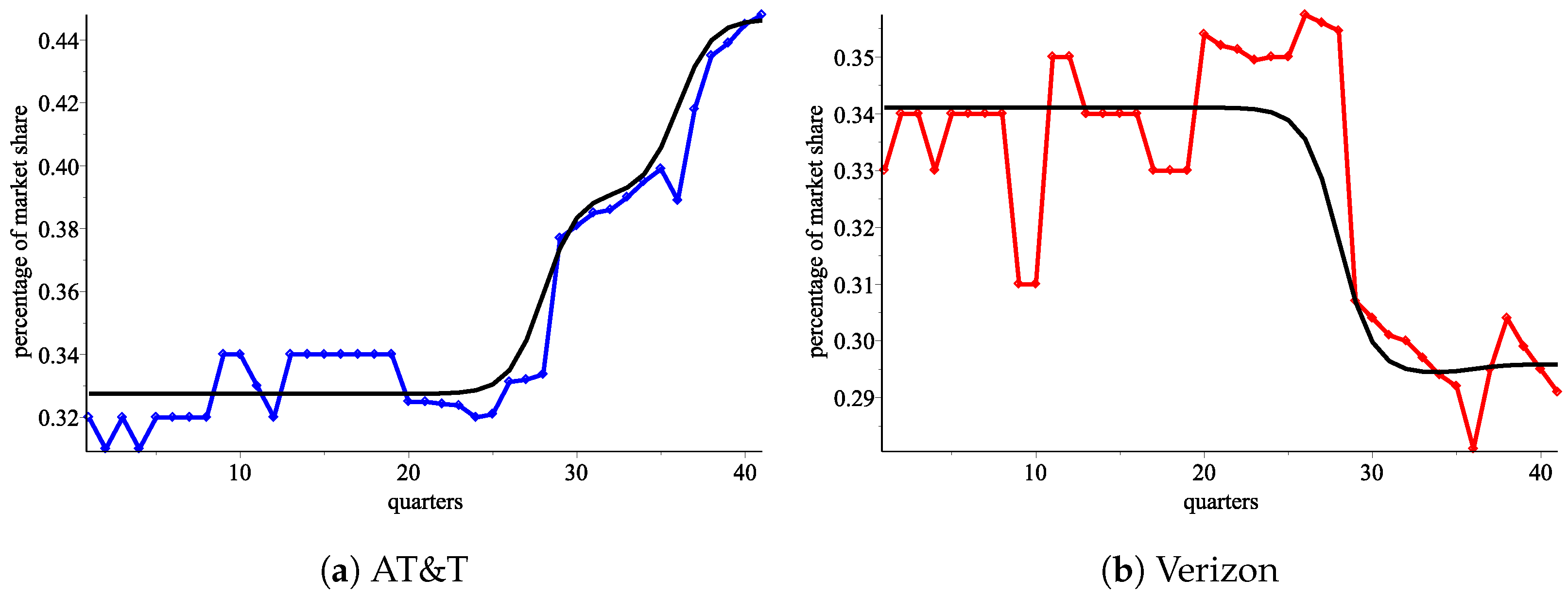
The resulting functions for the percentage presence of AT& T and Verizon by quarters over time are the following functions.

The function for AT&T is

$$S_1\left(t\right)=D+Ef\left(t\right)+Fg\left(t\right)=0.3275+0.0634\frac{1}{1+e^{28-t}}+0.0557\frac{1}{1+e^{36-t}}$$

and $D+E+F=0.4467$.

The function for $Verizon$ is

$$S_2\left(t\right)=A+B{f}_i\left(t\right)+C{g}_i\left(t\right)=0.3411-0.0469\frac{1}{1+e^{28-t}}+0.0017\frac{1}{1+e^{36-t}}$$

and $A+B+C=0.2958$.

The functions are plotted in Figure 3b and Figure 5a for $Verizon$ and $AT\&T$, respectively, where in black are the real data and in blue is the estimation, obtained.

We specifically note that the graphs are automatically scaled and vertically the curves appear more “stretched” than they would be on a real scale. In fact, the fluctuations of the real data around the approximating curves (in blue) are quite small, and the measurement accuracy is exactly 1 unit (1 percent) vertically, and any further rounding will distort the real data.

3.5. Constructing the Response Functions for the Alternative Model

We construct the response functions of AT&T and Verizon with the help of the sigmoid function in order to apply the technique from [1]. By repeating the calculation from above, we obtain the functions that present the numbers of mobile customers of each of the two biggest operators as sequences dependent of the time.

$$\begin{array}{c}{\displaystyle u_n=u\left(t_n\right)=139.925-\frac{116.028}{1+e^{\frac{t}{10}}}}\\ {\displaystyle v_n=v\left(t_n\right)=93.999-\frac{119.648}{1+e^{\frac{t}{10}-2}}}\end{array}$$

(9)

recursively, depending only on their values in the previous quarter (3-month period), where $u_n$ is the total number of consumers for AT& T and $v_n$ the total number for Verizon.

We search for functions $F_1$ and $G_1$ such that

$$u_n=u\left(t_n\right)=F_1(u_{n-1},v_{n-1}),$$

$$v_n=v\left(t_n\right)=G_1(u_{n-1},v_{n-1})$$

From (9) and taking into account that $t_n+1=t_{n+1}$, we obtain

$$\left|\begin{array}{c}{\displaystyle u_{n+1}=139.925-\frac{116.028}{1+e^{\frac{t_n+1}{10}}}}\hfill \\ {\displaystyle v_{n+1}=93.999-\frac{119.648}{1+e^{\frac{t_n+1}{10}-2}}}\hfill \\ {\displaystyle u_n=139.925-\frac{116.028}{1+e^{\frac{t_n}{10}}}}\hfill \\ {\displaystyle v_n=93.999-\frac{119.648}{1+e^{\frac{t_n}{10}-2}},}\hfill \end{array}\right.$$

(10)

which holds for any n. Transforming the third and fourth equations, we obtain

$$\left|\begin{array}{c}{\displaystyle u_{n+1}=139.925-\frac{116.028}{1+e^{\frac{t_n+1}{10}}}}\hfill \\ {\displaystyle v_{n+1}=93.999-\frac{119.648}{1+e^{\frac{t_n+1}{10}-2}}}\hfill \\ {\displaystyle t_n=20+10\ln \left(\frac{116.028}{139.925-u_n}-1\right)}\hfill \\ {\displaystyle t_n=10\ln \left(\frac{119.648}{93.999-v_n}-1\right).}\hfill \end{array}\right.$$

Substituting the third and fourth equations into the first and second by all possible combinations, we notice that

$$\left|\begin{array}{c}{\displaystyle u_{n+1}=1243.16-\frac{1345139.16}{1079.34+u_n}}\hfill \\ {\displaystyle u_{n+1}=3.48983+\frac{2870.98}{115.042-v_n}}\hfill \\ {\displaystyle v_{n+1}=1231.65-\frac{1430360.97}{1163.3+v_n}}\hfill \\ {\displaystyle v_{n+1}=110.695+\frac{2207.56}{7.70506-u_n}.}\hfill \end{array}\right.$$

Therefore, we arrive at the response functions

$$F_1(u,v)=1230.77+\frac{28.7098}{115.042-v}-\frac{1331687.77}{1079.34+u}$$

and

$$G_1(u,v)=1220.44-\frac{1416057.36}{1163.3+v}+\frac{22.0756}{7.70506-u}$$

as a consequence of (10).

Let $F_2$ and $G_2$ be the Taylor series of $F_1$ and $G_1$ to power 1 around the point $(u,v)=(89,140)$. Then, we obtain linear response functions for AT&T and Verizon

$$F_2(u,v)=8.53491+0.0641947v+0.895879u$$

$$G_2(u,v)=9.61236+0.895879v+0.00125026u,$$

respectively.

4. Model Fit

We proceed to statistically examine the model’s fit and to demonstrate that our model, based on the sigmoid approximation, delivers superior results in comparison to the direct estimation of response functions with low-degree polynomials by the least squares method.

4.1. The Least Squares Model

We employ an intuitive process using the obtained ordered pairs of response functions $(F,G)$, $(F_1,G_1)$ and $(F_2,G_2)$. Specifically, we calculate $(u_{n+1},v_{n+1})$ from

$$(F(u_{n+1},v_{n+1}),G(u_{n+1},v_{n+1}))$$

and

$$(u_{n+1},v_{n+1})=(F^{n+1}(u_0,v_0),G^{n+1}(u_0,v_0))$$

(Figure 6a,b).

According to the Pearson ${\chi }^2$ test, sequences ${\left\{F(u_n,v_n)\right\}}_{n=0}^{40}$ and ${\left\{G(u_n,v_n)\right\}}_{n=0}^{40}$ fit to the real data with p-values $99.1713\%$ and $67.5288\%$, respectively.

According to the Kolmogorov–Smirnov test, ${\left\{F(u_n,v_n)\right\}}_{n=0}^{40}$ and ${\left\{G(u_n,v_n)\right\}}_{n=0}^{40}$ fit to the real data with p-values $92.5652\%$ and $27.9043\%$, respectively.

According to the Pearson ${\chi }^2$ test, sequences ${\left\{F^n(u_{15},v_{15})\right\}}_{n=0}^{25}$ and ${\left\{G^n(u_{15},v_{15})\right\}}_{n=0}^{25}$ fit to the real data with p-values $23.781\%$ and $42.303\%$, respectively.

According to the Kolmogorov–Smirnov test, ${\left\{F^n(u_{15},v_{15})\right\}}_{n=0}^{25}$ and ${\left\{G^n(u_{15},v_{15})\right\}}_{n=0}^{25}$ fit to the real data with p-values $32.9008\%$ and $0.0000026531\%$, respectively. We can reject the hypothesis that ${\left\{(F^n(u_1,v_1),G^n(u_1,v_1))\right\}}_{n=0}^{40}$ fits the real-world data with the noted p-value, i.e., a high p-value implies good fit.

4.2. The Sigmoid Model

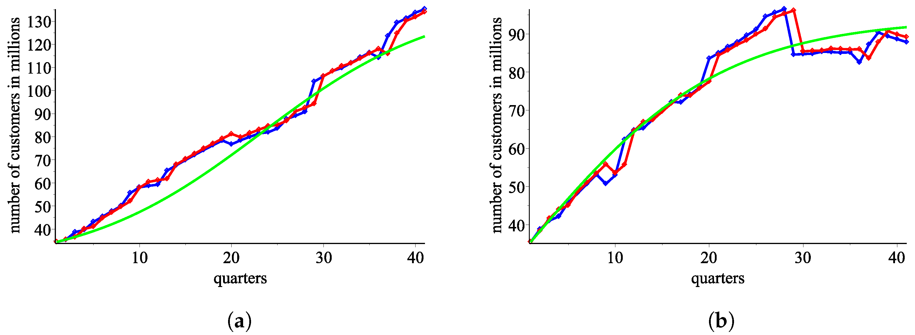
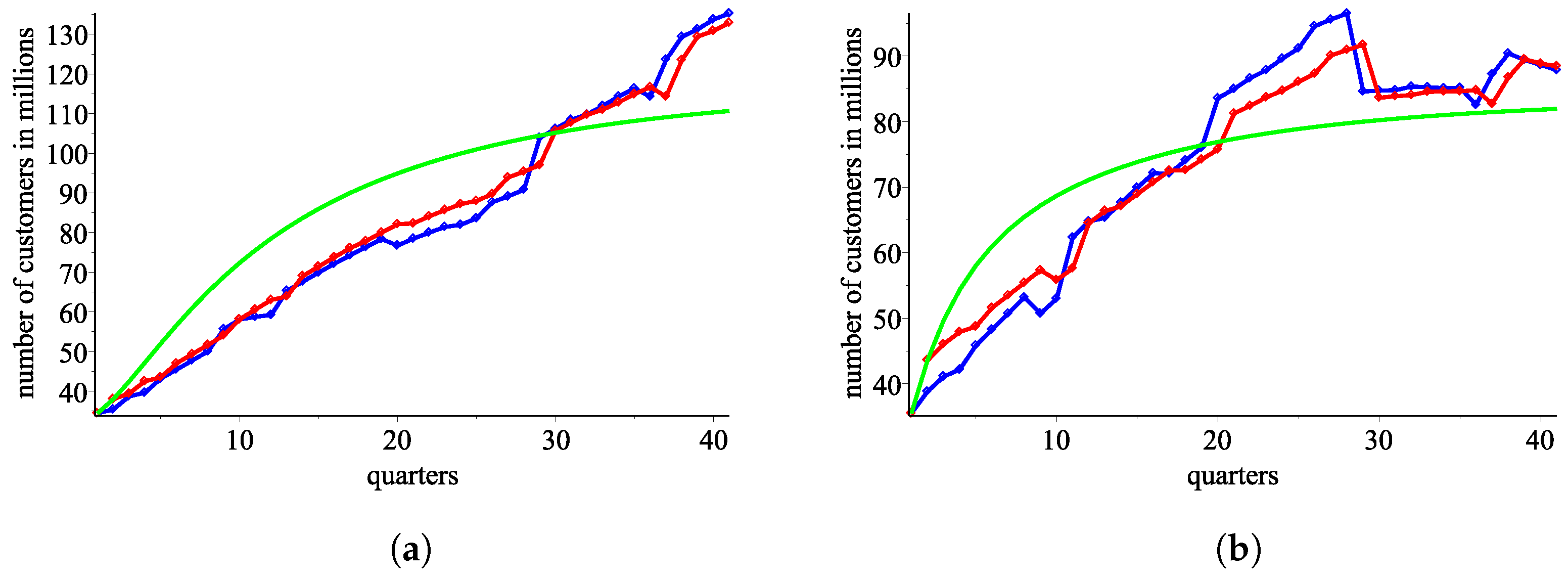
Using the response functions $(F_1,G_1)$ from the levels model, we plot the number of consumers for AT&T and Verizon, respectively (Figure 7a,b).

Using the response functions $(F_2,G_2)$ from the alternative model with market shares, we plot the number of consumers for AT&T and Verizon, respectively.

According to the Pearson ${\chi }^2$ test, sequences ${\left\{F_1(u_n,v_n)\right\}}_{n=0}^{40}$ and ${\left\{G_1(u_n,v_n)\right\}}_{n=0}^{40}$ fit to the real data with p-values $99.9189\%$ and $36.3436\%$, respectively.

According to the Kolmogorov–Smirnov test, ${\left\{F_1(u_n,v_n)\right\}}_{n=0}^{40}$ and ${\left\{G_1(u_n,v_n)\right\}}_{n=0}^{40}$ fit to the real data with p-values $99.9943\%$ and $59.4521\%$, respectively.

According to the Pearson ${\chi }^2$ test, sequences ${\left\{F_1^n(u_0,v_0)\right\}}_{n=0}^{40}$ and ${\left\{G_1^n(u_0,v_0)\right\}}_{n=0}^{40}$ fit to the real data with p-values $41.8444\%$ and $46.9134\%$, respectively.

According to the Kolmogorov–Smirnov test, ${\left\{F^n(u_0,v_0)\right\}}_{n=0}^{40}$ and ${\left\{G^n(u_0,v_0)\right\}}_{n=0}^{40}$ fit to the real data with p-values $92.5652\%$ and $99.1376\%$, respectively.

4.3. The Linear Approximation of the Sigmoid Model

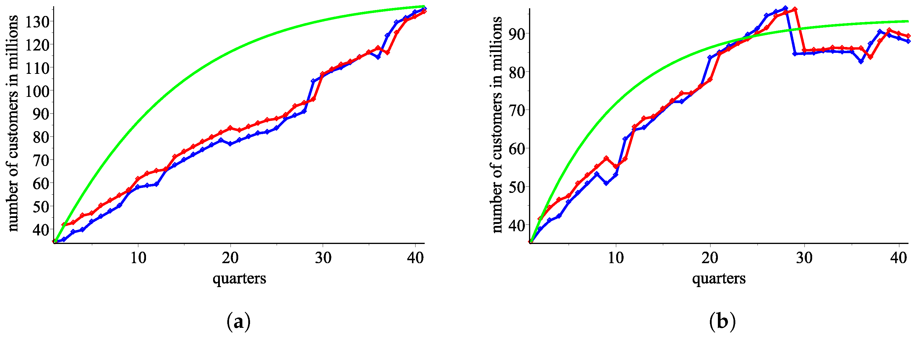
Using the response functions $(F_2,G_2)$ from the levels model, we plot the number of consumers for $AT\&T$ and $Verizon$, respectively (Figure 8a,b).

According to the Pearson ${\chi }^2$ test, sequences ${\left\{F_2(u_n,v_n)\right\}}_{n=0}^{40}$ and ${\left\{G_2(u_n,v_n)\right\}}_{n=0}^{40}$ fit to the real data with p-values $95.6712\%$ and $43.9697\%$, respectively.

According to the Kolmogorov–Smirnov test, ${\left\{F_2(u_n,v_n)\right\}}_{n=0}^{40}$ and ${\left\{G_2(u_n,v_n)\right\}}_{n=0}^{40}$ fits to the real data with p-values $92.5652\%$ and $59.4521\%$, respectively.

According to the Pearson ${\chi }^2$ test, sequences ${\left\{F^n(u_0,v_0)\right\}}_{n=0}^{40}$ and ${\left\{G^n(u_0,v_0)\right\}}_{n=0}^{40}$ fit to the real data with p-values $2.42453\%$ and $5.70819\%$, respectively.

According to the Kolmogorov–Smirnov test, ${\left\{F^n(u_0,v_0)\right\}}_{n=0}^{40}$ and ${\left\{G^n(u_0,v_0)\right\}}_{n=0}^{40}$ fit to the real data with p-values $0.153465\%$ and $10.4602\%$, respectively.

Note that only for four recursive sequences $(F^n(u_0,v_0),G^n(u_0,v_0))$ our modeling approach based on S-curves presents an approximation with a significant statistical confidence. Recursive approximations sometimes give bad results. The sigmoid approximation gives better fitting to the real data.

It is important to note that the Cournot model and the model of response functions actually are static models, i.e., we assume that there is no change in the external conditions in the market. So, we can conclude that probably there have been some changes in the external conditions (regulations or new technologies) and internal conditions (the market policy of the two players), which have changed the response functions, and thus the least squares method fits well for the quartiles $q_{26}$ to $q_{41}$.

5. Existence, Uniqueness and Stability of Market Equilibrium

We show that our empirical response functions $(F,G)$, $(F_1,G_1)$ and $(F_2,G_2)$ satisfy the hypothesis of Theorem 2 so that there exists a long-run equilibrium which is unique and stable. The next proposition is a simplification of the contractive-type condition that we need and is easy to check. Its proof is in the appendix.

Proposition 1. 

Let X and Y be two intervals in $\mathbb{R}$. Let the functions $f:X\times Y\to X$ and $g:X\times Y\to Y$ have continuous partial derivatives in $X\times Y$ such that

$${\displaystyle s_1=\sup \left\{\left|\frac{\partial f(u,v)}{\partial u}\right|+\left|\frac{\partial g(u,v)}{\partial u}\right|:u\in X,v\in Y\right\}<1}$$

and

$${\displaystyle s_2=\sup \left\{\left|\frac{\partial f(u,v)}{\partial v}\right|+\left|\frac{\partial g(u,v)}{\partial v}\right|:u\in X,v\in Y\right\}<1.}$$

Then, the ordered pair $(f,g)$ satisfies (3), i.e.,

$$|f(x,y)-f(u,v)|+|g(x,y)-g(u,v)|\le \max \{s_1,s_2\}\left(\right|x-u|+|y-v\left|\right).$$

Proof. 

Let $u,x\in X$ and $v,y\in Y$ be arbitrary points. Then, we can write for them

$$\begin{array}{ccc}{\displaystyle \left|f\right(x,y)-f(u,v\left)\right|}\hfill & =\hfill & {\displaystyle \left|f\right(x,y)-f(x,v)+f(x,v)-f(u,v\left)\right|}\hfill \\ \hfill & =\hfill & {\displaystyle \left|{\int }_v^y\frac{\partial f(x,t)}{\partial t}dt+{\int }_u^x\frac{\partial f(t,v)}{\partial t}dt\right|}\hfill \\ \hfill & \le \hfill & {\displaystyle \left|{\int }_v^y\left|\frac{\partial f(x,t)}{\partial t}\right|dt\right|+\left|{\int }_u^x\left|\frac{\partial f(t,v)}{\partial t}\right|dt\right|}\hfill \end{array}$$

(11)

Similarly, we obtain that

$${\displaystyle |g(x,y)-g(u,v)|\le \left|{\int }_v^y\left|\frac{\partial g(x,t)}{\partial t}\right|dt\right|+\left|{\int }_u^x\left|\frac{\partial g(t,v)}{\partial t}\right|dt\right|}$$

Adding this to (11), we can see that

$$\begin{array}{ccc}{S}_1\hfill & =\hfill & {\displaystyle \left|f\right(x,y)-f(u,v\left)\right|+\left|g\right(x,y)-g(u,v\left)\right|}\hfill \\ \hfill & \le \hfill & {\displaystyle \left|{\int }_v^y\left|\frac{\partial f(x,t)}{\partial t}\right|dt\right|+\left|{\int }_u^x\left|\frac{\partial f(t,v)}{\partial t}\right|dt\right|+\left|{\int }_v^y\left|\frac{\partial g(x,t)}{\partial t}\right|dt\right|+\left|{\int }_u^x\left|\frac{\partial g(t,v)}{\partial t}\right|dt\right|}\hfill \end{array}$$

(12)

Let us consider ${\displaystyle \left|{\int }_u^x\left|\frac{\partial f(t,v)}{\partial t}\right|dt\right|+\left|{\int }_u^x\left|\frac{\partial g(t,v)}{\partial t}\right|dt\right|}$. The functions we integrate are non-negative and the limits of the integrals are the same. Therefore,

$${\displaystyle \left|{\int }_u^x\left|\frac{\partial f(t,v)}{\partial t}\right|dt\right|+\left|{\int }_u^x\left|\frac{\partial g(t,v)}{\partial t}\right|dt\right|=\left|{\int }_u^x\left|\frac{\partial f(t,v)}{\partial t}\right|+\left|\frac{\partial g(t,v)}{\partial t}\right|dt\right|}$$

(13)

From the definition of $s_1$, it follows that ${\displaystyle \left|\frac{\partial f(t,v)}{\partial t}\right|+\left|\frac{\partial g(t,v)}{\partial t}\right|\le s_1}$ for every $t\in X$ and that $s_1\ge 0$. From this and (13), we obtain

$$\left|{\int }_u^x\left|\frac{\partial f(t,v)}{\partial t}\right|dt\right|+\left|{\int }_u^x\left|\frac{\partial g(t,v)}{\partial t}\right|dt\right|\le \left|{\int }_u^x{s}_{1}dt\right|=s_1|u-x|$$

(14)

Similarly, we can prove that

$$\left|{\int }_v^y\left|\frac{\partial f(x,t)}{\partial t}\right|dt\right|+\left|{\int }_v^y\left|\frac{\partial g(x,t)}{\partial t}\right|dt\right|\le s_2|v-y|$$

Let us substitute this and (14) in (12). Then, we obtain that

$$|f(x,y)-f(u,v)|+|g(x,y)-g(u,v)|\le s_1|u-x|+s_2|v-y|\le \lambda \left(\right|u-x|+|v-y\left|\right)$$

where $\lambda =\max \{s_1,s_2\}$, but from the definitions of $s_1$ and $s_2$, it follows that $0\le s_1<1$ and $0\le s_2<1$. Therefore, $0\le \lambda <1$, i.e., we obtain that for any $u,x\in X$ and $v,y\in Y$ we have

$$\left|f\right(x,y)-f(u,v\left)\right|+\left|g\right(x,y)-g(u,v\left)\right|\le \lambda \left(\right|u-x|+|v-y\left|\right)$$

where $0\le \lambda <1$. □

We will show that the assumptions in Theorem 2 are satisfied by the response functions’ ordered pairs $(F,G)$, $(F_1,G_1)$ and $(F_2,G_2)$.

It is easy to check that

$$\max \left\{F\right(u,v):u\in [0,90],v\in [0,143\left]\right\}<89.99=F(90,143),$$

$$\min \left\{F\right(u,v):u\in [0,90],v\in [0,143\left]\right\}>16.32=F(0,0)$$

$$\max \left\{G\right(u,v):u\in [0,90],v\in [0,143\left]\right\}<142.99=G(90,143)$$

and

$$\min \left\{G\right(u,v):u\in [0,90],v\in [0,143\left]\right\}>3.92=G(0,0).$$

After calculating

$${\alpha }_1=\sup \left\{\left|\frac{\partial F}{\partial u}(u,v)\right|+\left|\frac{\partial G}{\partial u}(u,v)\right|:u\in A,v\in B\right\}\le 0.993,$$

$${\alpha }_2=\sup \left\{\left|\frac{\partial F}{\partial v}(u,v)\right|+\left|\frac{\partial G}{\partial v}(u,v)\right|:u\in A,v\in G\right\}=0.99$$

we obtain that the ordered pair $(F,G)$ satisfies Proposition 1. Consequently, there is a unique market equilibrium pair $(\xi ,\eta )$ in $D=A\times B$, i.e., $\xi =F(\xi ,\eta )$ and $\eta =G(\xi ,\eta )$. Moreover, for any market initial conditions $(x_0,y_0)\in A\times B$, the sequence of successive responses of productions $x_n=F^n(x_n,y_n)$ and $y_n=G^n(x_n,y_n)$ converge to $(\xi ,\eta )$, and they hold the error estimates from Theorem 2.

By solving $u=F(u,v),v=G(u,v)$, we obtain the solutions $u=89.99964717$, $v=142.9986486$, $u=93.91152837$, $v=162.4557731$ and several solutions with $u<0$ and/or $v<0$. From the fact that $F:[0,90]\times [0,143]\to [0,90]$ and $G:[0,90]\times [0,143]\to [0,143]$, it follows that the market equilibrium is attained for productions $u=89.99964717$, $v=142.9986486$.

Let $U=[85,140]$ and $V=[85,94]$. Then, we can calculate that $F_1(U,V)\subseteq U$ and $G_1(U,V)\subseteq V$. Also, we can calculate that

$${\displaystyle {\beta }_1=\sup \left\{\left|\frac{\partial F_1}{\partial u}(u,v)\right|+\left|\frac{\partial G_1}{\partial u}(u,v)\right|:u\in U,v\in V\right\}=0.98599}$$

and

$${\displaystyle {\beta }_2=\sup \left\{\left|\frac{\partial F_1}{\partial v}(u,v)\right|+\left|\frac{\partial G_1}{\partial v}(u,v)\right|:u\in U,v\in V\right\}=0.96063.}$$

From Proposition 1, it follows that the ordered pair $(F_1,G_1)$ satisfies Theorem 2 in $[85,140]\times [85,95]$ with $\lambda =0.98599$. By solving $u=F(u,v),v=G(u,v)$, we obtain several solutions, but just one of them, $u=139.99, v=94.04$, lies in $[85,140]\times [85,95]$.

Let $U=[0,140]$ and $V=[0,94]$. Then, we can calculate that $F_2(U,V)\subseteq U$ and $G_2(U,V)\subseteq V$. Also, we can calculate that

$${\displaystyle {\gamma }_1=\sup \left\{\left|\frac{\partial F_2}{\partial u}(u,v)\right|+\left|\frac{\partial G_2}{\partial u}(u,v)\right|:u\in U,v\in V\right\}=0.897129}$$

and

$${\displaystyle {\gamma }_2=\sup \left\{\left|\frac{\partial F_2}{\partial v}(u,v)\right|+\left|\frac{\partial G_2}{\partial v}(u,v)\right|:u\in U,v\in V\right\}=0.960073}$$

From Proposition 1, it follows that the ordered pair $(F_2,G_2)$ satisfies Theorem 2 in $[0,140]\times [0,94]$ with $\lambda =0.960073$. By solving $u=F(u,v),v=G(u,v)$, we obtain the solutions $u=139.9253568$, $v=93.99931884$. We see that the linear approximation of the sigmoid functions satisfies Theorem 2 with intervals with greatest length.

Besides the best statistical fitting of the model to the real data, when sigmoid functions are used, the response functions

$$F_1(u,v)=1230.77+\frac{28.7098}{115.042-v}-\frac{1331687.77}{1079.34+u}$$

and

$$G_1(u,v)=1220.44-\frac{1416057.36}{1163.3+v}+\frac{22.0756}{7.70506-u}$$

give us more information on the responses of the two players. For example, let us consider player one. With the response function $F_1$, it is an increasing and concave function of u, i.e., any good results $u_1<u_2$ lead to an increase in market results, but as u becomes bigger and bigger, the increment becomes less and less.

For player two, from $G_2$ we see that a small value of $u\ge 8$, i.e., the number of consumers of player one, leads to a decrease in the market results for player two.

6. Using the Empirical Response Functions to Simulate Convergence to the Equilibrium

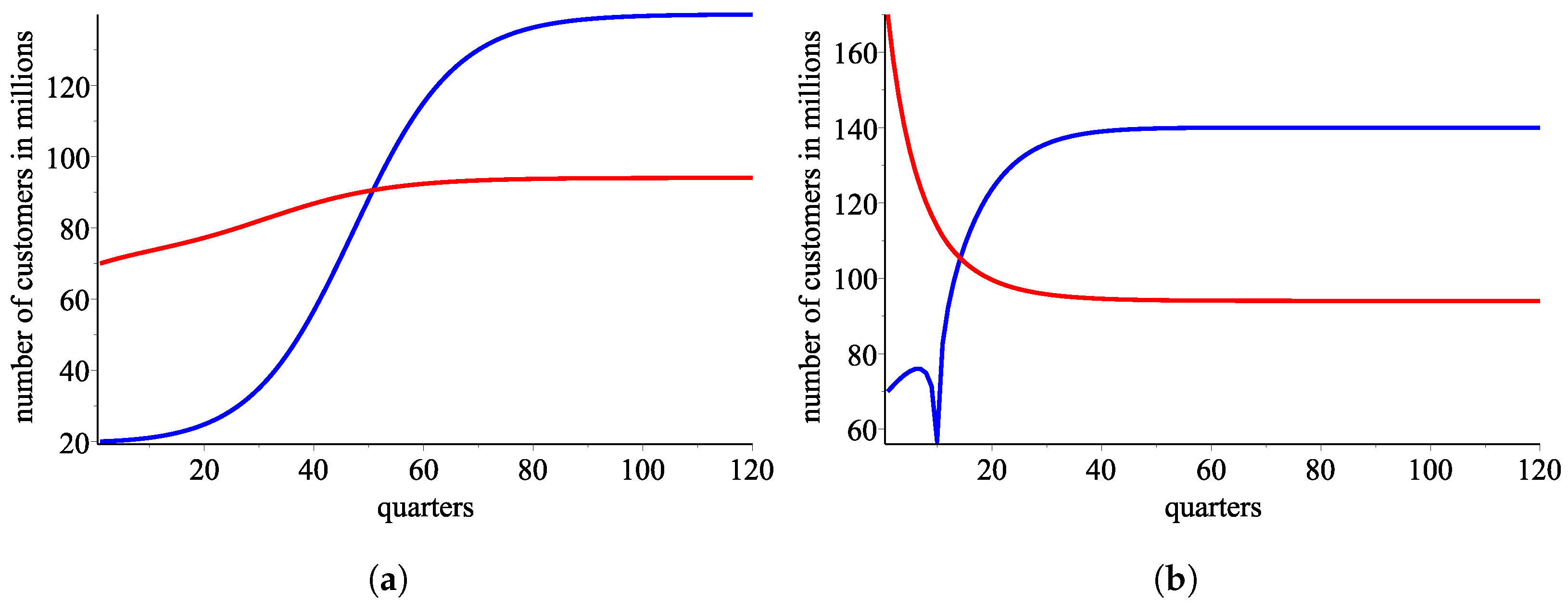
This section illustrates with numerical simulations how our empirical response functions converge to the long-run equilibrium. Specifically, we experiment with initial values that are significantly different from the actual data and that are outside the range where we can invoke Theorem 2, i.e., for which we know with certainty that the responses converge to the long-run equilibrium.

Figure 9a and Figure 9b plot the sequences of successive market outcomes if the initial start is $(20,70)$ and $(70,170)$, respectively, approximated with the sigmoidal response functions $(F1,G1)$.

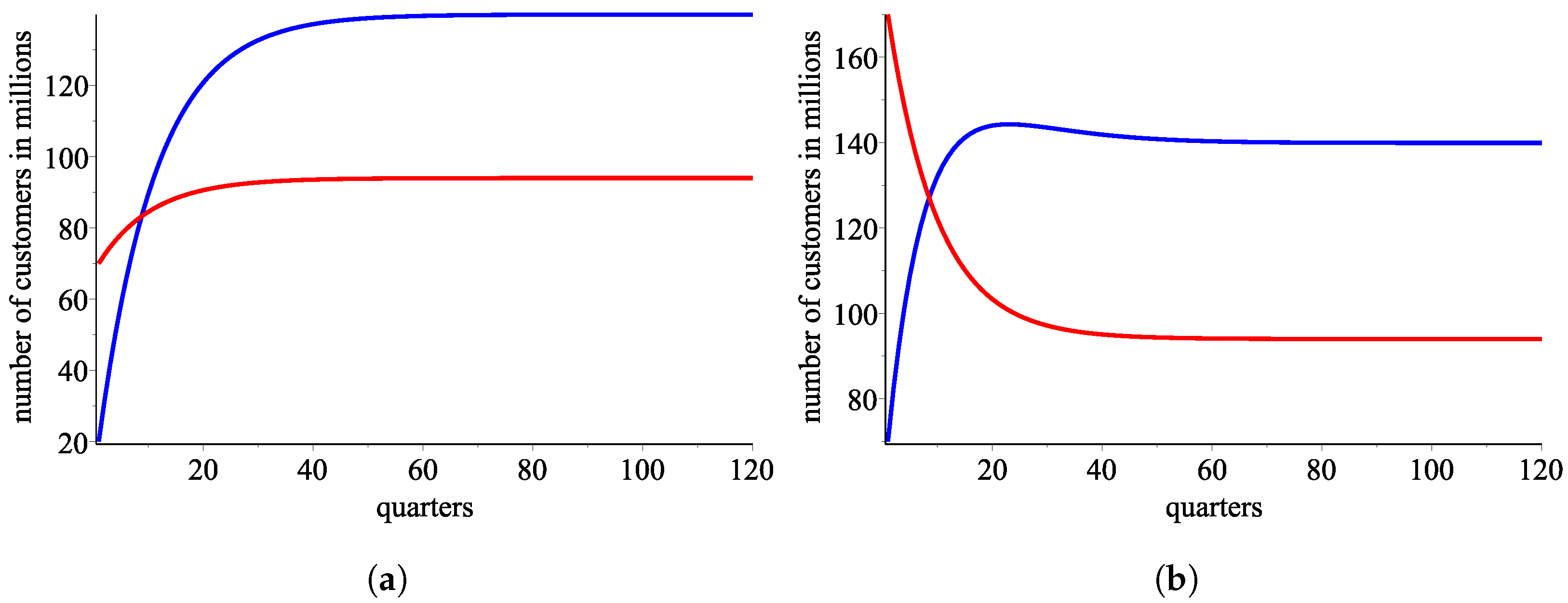
Figure 10a and Figure 10b plot the predicted market path if the initial start is $(20,70)$ and $(70,170)$, respectively, approximated with the sigmoidal response functions $(F2,G2)$.

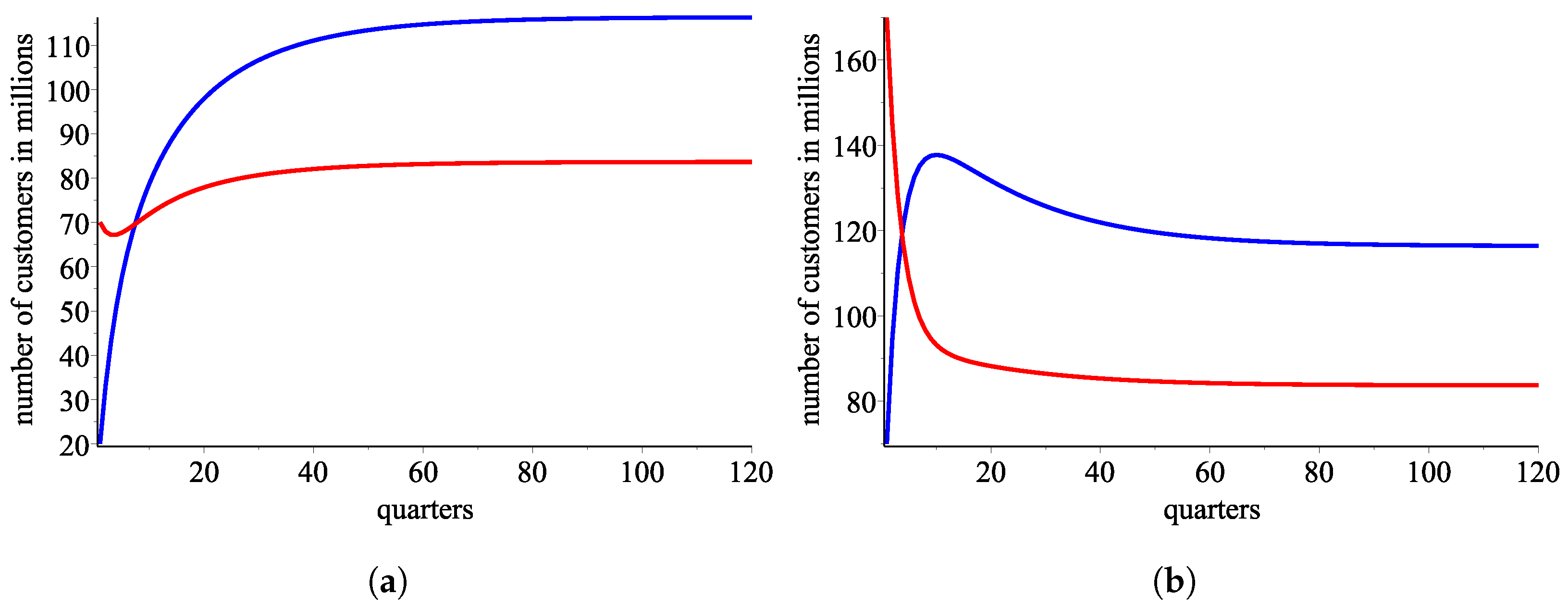
Figure 11a and Figure 11b illustrate the evolution of the market if the initial start is $(20,70)$ and $(70,170)$, respectively, approximated with the sigmoidal response functions $(F,G)$.

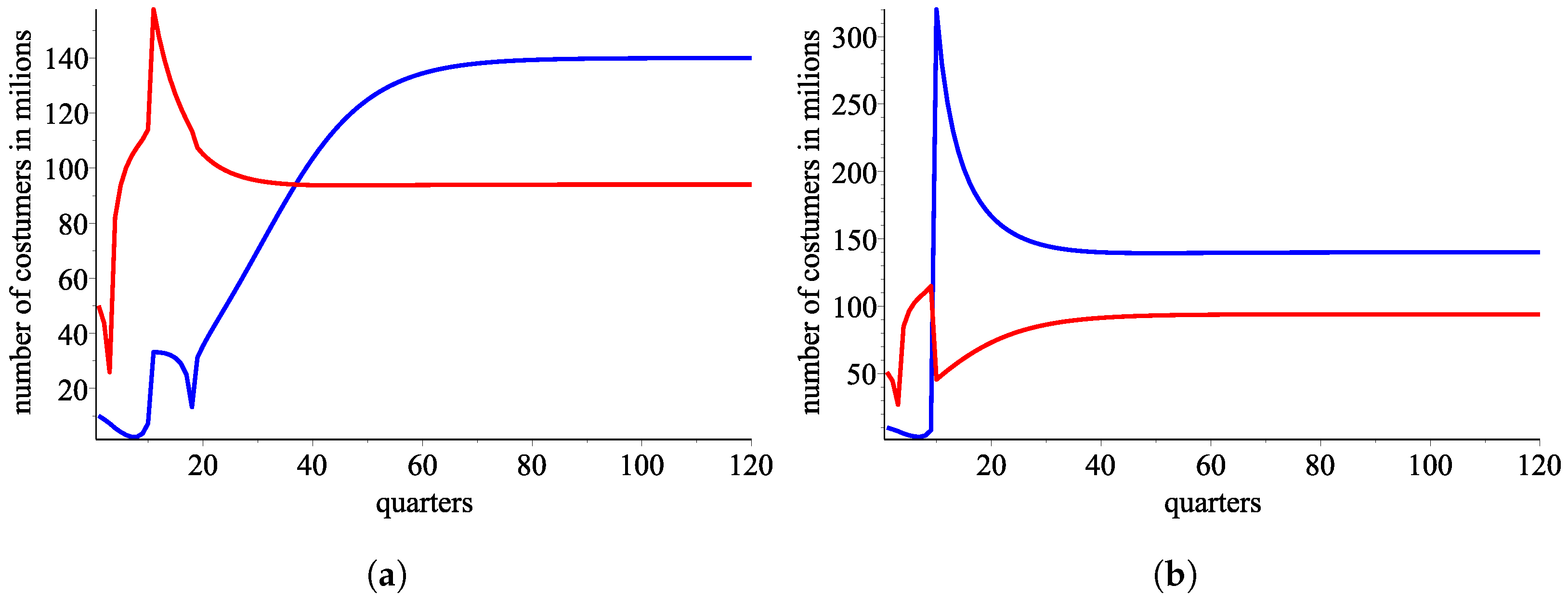
Finally, in Figure 12a and Figure 12b, the starting values are $(10,50)$ and $(10,51)$, respectively, and the market evolution is approximated with the sigmoidal response functions $(F_1,G_1)$.

Our numerical analysis demonstrates that the long-run equilibrium is stable even when the initial conditions are not in the set where we can rely on the conclusion of Theorem 2. We note in passing that the response functions generated with the least squares method do not demonstrate stability for this wide range of initial conditions.

7. Conclusions

We empirically study the wireless telecommunication market in the USA using an equilibrium theory based on response functions instead of a payoff maximization problem. In our settings, the approximation technique using sigmoid functions gives slightly better results in comparison to the classical least squares method. It is worth noting that the linear approximation of the sigmoid model approaches the linear part in the function obtained by the method of least squares. All in all, this is an illustration of the framework to model market equilibrium via response functions introduced in [1,10],

Numerical simulations from our robustness analysis suggest that the conditions imposed in Theorem 2 are only sufficient. Even with an initial state of the economy, for which we cannot formally guarantee the convergence of the empirical response functions, the market converges to long-run equilibrium. This observation is reaffirming in offering confidence that our approach delivers an adequate description of the evolution of the market.

More generally, our approach is applicable to other settings. If we assume that the participants in the duopoly market behave rationally and we know their cost functions, then from (2) we can model for the inverse demand function P. Further, we can model the cost functions of the two participants once we know the demand function.

Our model is simplified on purpose. Indeed, it is possible to look for a functional relationship between several products offered on the market by the two participants, or even to match each product k with an ordered pair of quantity and price $(x_k,p_k)$, $k=1,2,\cdots n$, and examine the presence of equilibrium with the help of response functions $F_i((x_1,p_1),(x_2,p_2),\dots ,(x_n,p_n))$, $i=1,2$.

References

- Stanimir, K.; Zhelinski, V.; Zlatanov, B. Coupled Fixed Points for Hardy–Rogers Type of Maps and Their Applications in the Investigations of Market Equilibrium in Duopoly Markets for Non-Differentiable, Nonlinear Response Functions. Symmetry 2022, 14, 605. [Google Scholar] [CrossRef]
- Augustin, C.A. Researches into the Mathematical Principles of the Theory of Wealth, Translation ed.; Macmillan: New York, NY, USA, 1897. [Google Scholar]
- Rubinstein, A. Modeling Bounded Rationality; MIT Press: Cambridge, UK, 2019. [Google Scholar]
- Ueda, M. Effect of information asymmetry in Cournot duopoly game with bounded rationality. Appl. Math. Comput. 2019, 362, 124535. [Google Scholar] [CrossRef]
- Cellini, R.; Lambertini, L. Dynamic oligopoly with sticky prices: Closed-loop, feedback and open-loop solutions. J. Dyn. Control Syst. 2004, 10, 303–314. [Google Scholar] [CrossRef]
- Friedman, J.W. Oligopoly Theory; Cambradge University Press: Cambradge, UK, 2007. [Google Scholar]
- Bischi, G.I.; Chiarella, C.; Kopel, M.; Szidarovszky, F. Nonlinear Oligopolies Stability and Bifurcations; Springer: Berlin/Heidelberg, Germany, 2010. [Google Scholar] [CrossRef]
- Matsumoto, A.; Szidarovszky, F. Dynamic Oligopolies with Time Delays; Springer: Singapore, 2018. [Google Scholar] [CrossRef]
- Okuguchi, K.; Szidarovszky, F. The Theory of Oligopoly with Multi–Product Firms; Springer: Berlin/Heidelberg, Germany, 1990. [Google Scholar] [CrossRef]
- Dzhabarova, Y.; Kabaivanov, S.; Ruseva, M.; Zlatanov, B. Existence, Uniqueness and Stability of Market Equilibrium in Oligopoly Markets. Adm. Sci. 2020, 10, 70. [Google Scholar] [CrossRef]
- Andaluz, J.; Elsadany, A.A.; Jarne, G. Dynamic Cournot oligopoly game based on general isoelastic demand. Nonlinear Dyn. 2020, 99, 1053–1063. [Google Scholar] [CrossRef]
- Okuguchi, K. Expectations and Stability in Oligopoly Models; Springer: Berlin/Heidelberg, Germany, 1976. [Google Scholar] [CrossRef]
- Alavifard, F.; Ivanov, D.; He, J. Optimal divestment time in supply chain redesign under oligopoly: Evidence from shale oil production plants. Int. Trans. Oper. Res. 2020, 27, 2559–2583. [Google Scholar] [CrossRef]
- Geraskin, M. The properties of conjectural variations in the nonlinear stackelberg oligopoly model. Autom. Remote. Control 2020, 81, 1051–1072. [Google Scholar] [CrossRef]
- Siegert, C.; Robert, U. Dynamic oligopoly pricing: Evidence from the airline industry. Int. J. Ind. Organ. 2020, 71, 102639. [Google Scholar] [CrossRef]
- Strandholm, J.C. Promotion of green technology under different environmental policies. Games 2020, 11, 32. [Google Scholar] [CrossRef]
- Xiao, G.; Wang, Z. Empirical study on bikesharing brand selection in china in the post-sharing era. Sustainability 2020, 12, 3125. [Google Scholar] [CrossRef]
- Baik, K.H.; Lee, D. Decisions of duopoly firms on sharing information on their delegation contracts. Rev. Ind. Organ. 2020, 57, 145–165. [Google Scholar] [CrossRef]
- Liu, Y.; Sun, M. Application of duopoly multi-periodical game with bounded rationality in power supply market based on information asymmetry. Appl. Math. Model. 2020, 87, 300–316. [Google Scholar] [CrossRef]
- Xia, W.; Shen, J.; Sheng, Z. Asymmetric model of the quantum Stackelberg duopoly with incomplete information. Phys. Lett. A 2020, 384, 126644. [Google Scholar] [CrossRef]
- Banach, S. Sur les opérations dan les ensembles abstraits et leurs applications aux integrales. Fundam. Math. 1922, 3, 133–181. [Google Scholar] [CrossRef]
- Guo, D.; Lakshmikantham, V. Coupled fixed points of nonlinear operators with applications. Nonlinear Anal. Theory Methods Appl. 1987, 11, 623–632. [Google Scholar] [CrossRef]
- Bhaskar, T.G.; Lakshmikantham, V. Fixed point theorems in partially ordered metric spaces and applications. Nonlinear Anal. 2006, 65, 1379–1393. [Google Scholar] [CrossRef]
- Petruşel, A. Fixed points vs. coupled fixed points. J. Fixed Point Theory Appl. 2018, 20, 150. [Google Scholar] [CrossRef]
- Kirk, W.; Srinivasan, P.; Veeramani, P. Fixed points for mappings satisfying cyclical contractive condition. Fixed Point Theory 2003, 4, 179–189. [Google Scholar]
- Sintunavarat, W.; Kumam, P. Coupled best proximity point theorem in metric spaces. Fixed Point Theory Appl. 2012, 2012, 93. [Google Scholar] [CrossRef]
- Zlatanov, B. Coupled best proximity points for cyclic contractive maps and their applications. Fixed Point Theory 2021, 22, 431–452. [Google Scholar] [CrossRef]
- Ajeti, L.; Ilchev, A.; Zlatanov, B. On Coupled Best Proximity Points in Reflexive Banach Spaces. Mathematics 1992, 10, 1304. [Google Scholar] [CrossRef]
- Cybenko, G. Approximation by superpositions of a sigmoidal function. Math. Control Signals Syst. 1989, 2, 303–314. [Google Scholar] [CrossRef]
- Carr, A.C.; Lykkesfeldt, J. Factors Affecting the Vitamin C Dose-Concentration Relationship: Implications for Global Vitamin C Dietary Recommendations. Nutrients 2023, 15, 1657. [Google Scholar] [CrossRef]
- Eid, E.M.; Keshta, A.; Alrumman, S.; Arshad, M.; Shaltout, K.; Ahmed, M.; Al-Bakre, D.; Alfarhan, A.; Barcelo, D. Modeling Soil Organic Carbon at Coastal Sabkhas with Different Vegetation Covers at the Red Sea Coast of Saudi Arabia. J. Mar. Sci. Eng. 2023, 11, 295. [Google Scholar] [CrossRef]
- Gobin, A.; Sallah, A.-H.M.; Curnel, Y.; Delvoye, C.; Weiss, M.; Wellens, J.; Piccard, I.; Planchon, V.; Tychon, B.; Goffart, J.P.; et al. Crop Phenology Modelling Using Proximal and Satellite Sensor Data. Remote Sens. 2023, 15, 2090. [Google Scholar] [CrossRef]
- Krishnasamy, S.; Alotaibi, M.; Alehaideb, L.; Abbas, Q. Development and Validation of a Cyber-Physical System Leveraging EFDPN for Enhanced WSN-IoT Network Security. Sensors 2023, 23, 9294. [Google Scholar] [CrossRef] [PubMed]
- Martínez Pérez, A.; Pérez Martín, P.S. Logistic regression. Semergen 2024, 80, 102086. [Google Scholar] [CrossRef] [PubMed]
- Debecker, A.; Modis, T. Determination of the Uncertainties in S-Curve Logistic Fits. Technol. Forcasting Soc. Chang. 1994, 46, 153–173. [Google Scholar] [CrossRef]
- Mitchell, T. Machine Learning; McGraw-Hill International Editions Computer Science Series; McGraw-Hill: New York, NY, USA, 1997. [Google Scholar]
- Jan, C. The early origins of the logit model. Stud. Hist. Philos. Sci. Part C Stud. Hist. Philos. Biol. Biomed. Sci. 2004, 35, 613–626. [Google Scholar] [CrossRef]
Figure 1.
A sigmoid function.
Figure 2.
A few basic sigmoid functions: , , and .
Figure 3.
Percentage shares in the mobile market in the USA. (a) Graphic data for the seven mobile operators in the USA (2009–2020). (b) Graphic data for the two biggest operators, AT&T in blue and Verizon in red (2009–2020).
Figure 4.
Total number of mobile users (2009–2020) and their approximation by the sigmoid function .
Figure 5.
A sigmoid approximation of the percentage as a function of the time.
Figure 6.
An approximation from using the ordered pair of response functions . (a) AT&T: blue—the real data, red—an approximation using , green—an approximation using . (b) Verizon: blue—the real data, red—an approximation using , green—an approximation using .
Figure 7.
Figure 8.
An approximation from using the ordered pair of response functions . (a) : blue—the real data, red—an approximation using , green—an approximation using . (b) : blue—the real data, red—an approximation using , green—an approximation using .
Figure 9.
A simulation with the ordered pair of response functions (blue color for customers of AT&T and red color for Verizone ones) (a) Evolution of the market with the sigmoid model if the initial start is . (b) Evolution of the market with the sigmoid model if the initial start is .
Figure 10.
A simulation with the ordered pair of response functions (blue color for customers of AT&T and red color for Verizone ones) (a) Evolution of the market with the linear approximation of the sigmoid model if the initial start is . (b) Evolution of the market with linear approximation of the sigmoid model if the initial start is .
Figure 11.
A simulation with the ordered pair of response functions (blue color for customers of AT&T and red color for Verizone ones) (a) Evolution of the market with the least square model if the initial start is . (b) Evolution of the market with the least square model if the initial start is .
Figure 12.
A simulation with the ordered pair of response functions .