Abstract
The problem of the approximation of the coefficients of the objective function of a scheduling problem for a single machine is considered. It is necessary to minimize the total weighted completion times of jobs with unknown weight coefficients when a set of problem instances with known optimal schedules is given. It is shown that the approximation problem can be reduced to finding a solution to a system of linear inequalities for weight coefficients. For the case of simultaneous job release times, a method for solving the corresponding system of inequalities has been developed. Based on it, a polynomial algorithm for finding values of weight coefficients that satisfy the given optimal schedules was constructed. The complexity of the algorithm is operations, where n is the number of jobs and N is the number of given instances with known optimal schedules. The accuracy of the algorithm is estimated by experimentally measuring the function , which is an indicator of the average modulus of the relative deviation of the found values from the true values . An analysis of the results shows a high correlation between the dependence and a function of the form , where is a decreasing function of n.
Keywords:
scheduling theory; single machine scheduling; total weighted completion times; approximation MSC:
90B35
1. Introduction
Scheduling theory is a branch of discrete optimization devoted to planning operations over time. The problems of scheduling theory are diverse, including, but not limited to, production scheduling, including human-robot collaborations [1], classical Resource-Constrained Project Scheduling Problem (RCPSP) [2], creating smart planning eco-systems [3], distributed scheduling problems [4], and dynamic systems [5]. However, classical problems for a single machine remain relevant, still capture the attention of the scientific community [6] and are also used in modern approaches of Industry 4.0 [7].
In the classical single-machine scheduling problem, there is a set of jobs with given release times, processing times and due dates. The goal is to schedule the jobs to proceed on the machine, minimizing some objective functions. A wide variety of studies of this problem can be found for such objective functions as the total or maximum lateness [8,9], the weighted number of tardy jobs [10], the total (weighted) completion time [11,12] or any arbitrary non-decreasing function of the completion time [13]. The idea is that the objective function is known and should be maximized or minimized.
In practice, the quality criterion and, therefore, the objective function are not defined for some applied scheduling problems. Let some optimal schedules be pre-given. The goal is to construct an optimal schedule for the new input data and to estimate unknown objective function. To apply the methods of scheduling theory to this problem, it is necessary to determine the objective function. The task of the objective function approximation arises as a sub-task in the scheduling automation process, so the approximation algorithm must be fast enough compared to the required frequency of scheduling. An indicator of the quality of the approximation algorithm is the quality of the schedule obtained for the approximated objective function.
A linear approximation for a single-machine scheduling problem is considered: it is assumed that there exists an objective function that is linear in job-weighted completion times, and the previously constructed schedules are optimal with respect to this objective function. The initial problem is reduced to solving a system of linear inequalities with respect to the unknown values of the weight coefficients of the objective function. A detailed review of the results of the algebraic theory of linear inequalities was given by [14], which also includes an algorithm for finding a general formula for non-negative solutions of [15], based on the principle of boundary solutions. General results on this topic were also presented by [16,17], who also used some properties of convex cones in the solution space. Refs. [18,19] obtained results for a set of solutions (redundancy and dimension) of a certain class of systems of inequalities–normal systems.
The main contribution of this paper is an algorithm for approximating the weight coefficients for the case of simultaneous job release times. The system of linear inequalities in this case has a sparse matrix (most of the elements are zero), which contains a significant number of dependent inequalities. The solution method is primarily based on the exclusion of dependent inequalities from the system and using some general properties of linear inequality systems.
The structure of this paper is organized as follows. In Section 2 the mathematical formulation of the problem will be given and thereupon mathematical statement of the problem of approximation of objective function weight coefficients is formulated; in Section 3 a method for solving the problem is proposed; in Section 4 a numerical study of the constructed approximation algorithm is carried out and its final complexity is calculated. Section 5 contains a brief conclusion.
2. Mathematical Problem Formulation
The problem studied in this article is in some way the inverse of one of the classic problems in scheduling theory, the problem of minimizing the total weighted completion time . To describe the main problem, problem should be introduced first. There is a single machine and a set of n jobs that need to be processed on the machine. For each job , the release time and processing time are given. There are no precedence relations of jobs, and interruptions of the job processing are prohibited. The order in which the jobs are processed is called a schedule. In problem , it is necessary to find a schedule minimizing the total weighted completion time , where is the completion time of job j, and is a weight coefficient of the completion time of the corresponding job j. Completion times of jobs under schedule are defined as follows:
Remark 1.
The case of problem with zero weight coefficients can be solved trivially: all corresponding jobs are processed last and are excluded from the consideration. The case with negative weight coefficients does not make sense from a practical point of view. In this regard, it is assumed in this paper that all weight coefficients are positive.
Remark 2.
Note, that the problem about the total weighted lateness , where is the due date for job , is equivalent to problem and the optimal schedule in problem does not depend on the values of due dates . Further, the problem will be considered, implying that all the results obtained can be applied to the problem .
Definition 1.
A set of job release times and processing times is called a problem instance I of problem
The general case of problem with weight coefficients is -hard in the strong sense [20]. An analysis of the approaches and methods for solving single-machine scheduling problems can be found in [21]. According to generalized Smith theorem [22], a polynomially solvable special case of problem is problem , in which, despite the general case, a simultaneous release times are assumed. An optimal schedule in this case will be a schedule constructed in order of non-decreasing values .
Definition 2.
A set of job processing times is called a problem instance I of problem
Now, the problem of approximation of objective function weight coefficients can be formulated as follows.
Problem 1.
N instances of the problem (or the problem in the general case) are given, and corresponding optimal schedules are known. The goal is to approximate values of unknown weight coefficients .
Thus, the problem considered in this paper is inverse to the problem . A linear approximation is considered for the problem for a single machine: it is assumed that there is an objective function that is linear with respect to the completion times, the optimal schedule is known, but the weight coefficients of the objective function are unknown. This problem may arise, for example, at the initial stages of automating individual processes at enterprises where there is a long experience in scheduling “manually”, but modeling the entire production process and the analytical formulation of the optimality criterion is, for some reason, impossible or not obvious.
3. Approximation Problem Solving Method
The method for solving the problem of approximating weight coefficients (both for general and for particular cases) is based on determining the optimality of schedules :
Therefore,
Thus, the values of are generally determined by a system of inequalities of the form (1), i.e., the dependence of the number of inequalities in the system on the number of jobs is not polynomial, because for any instance there are possible schedules. The non-polynomial complexity of the approximation algorithm can be avoided if among the inequalities there is a polynomial number m of independent ones, while the remaining inequalities are consequences of these m inequalities.
In case the following approximation problem can be considered: one instance I of problem of dimension n is given, i.e., for n jobs, the release times and processing times are defined, and the optimal schedule is also known. Then, for an arbitrary acceptable schedule the following inequality holds:
Repeating the arguments about the non-polynomial number of inequalities, the following proposition can be formulated. The proposition is sufficient for the polynomial approximation algorithm.
Proposition 1.
For an arbitrary instance I of problem in a system of inequalities of the form (2) there is a subsystem of m inequalities, the solution of which coincides with the solution of the initial system, and the number m depends polynomially on n.
Each of the strict inequalities of the form (2) corresponds to some non-optimal schedule . In this case, Proposition 1 means that among non-optimal schedules there are m schedules such that the solution of this system of inequalities of the form (2) corresponding to the schedules , coincides with the solution of the initial system, and the number m depends polynomially on n. In other words, for any schedule , an inequality of the form (2) corresponding to schedule is a consequence of the system of inequalities corresponding to schedules . Finding proof (or inconsistency) of the Proposition 1 is the key to solving the approximation problem for the .
3.1. The Initial and Efficient System of Inequalities for the Problem
Consider approximating the weight coefficients of the problem . According to the generalized Smith theorem [22], for problem instance of there exists an optimal schedule , for which
Remark 3.
If one or more adjacent non-strict inequalities of set (3) turn into equality, that is, the ratios are equal for jobs , all those schedules are also optimal, in which the jobs are placed in any other arbitrary order :
An inequality of the form (3) is valid for all N given instances of the problem and the corresponding optimal schedules .
Definition 3.
The system of inequalities for weight coefficients
we will call the initial system of inequalities of the problem of approximation of weight coefficients for the case .
The initial system (4) contains inequalities. To reconstruct the system to a more convenient form for solving, the following notation will be used.
Let be the set of indices corresponding to the given pairs of problem instances and their optimal schedules, and let be some subset of the set K. Further, the record of the form
will mean the minimum (maximum) for all possible pairs such that .
For an arbitrary pair of jobs the set K can be divided into two subsets and depending on the relative position of the jobs in the schedule :
Then, from the inequalities (4) of the initial system for the corresponding weight coefficients the following inequalities can be constructed:
or, more conveniently,
Remark 4.
Let
then the system of inequalities (5a) and (5b) for the chosen is equivalent to the double inequality:
Remark 5.
Consider the case when one of the sets is empty. Let, for example, , that is, there were no inequalities of the form (5a) in the initial system. In this case, it will be assumed that for the uniformity of the algorithm, and the inequality (6) will have form
Similarly, if , then it will be assumed that and the inequality (6) will have form
Jobs were chosen arbitrarily; therefore, the inequality (6) can be written for any pair of different jobs .
Definition 4.
A system of inequalities
where:
- we call the efficient system of inequalities of the weight coefficient approximation problem for the case .
Proof.
The efficient system is the result of equivalent transformations of the inequalities of the initial system and, taking into account the Remark 4, includes all the inequalities of the initial system related to , for all possible pairs , , that is, it contains all the inequalities of the initial system. Therefore, the efficient system of inequalities is equivalent to the initial system. □
Thus, the solution sets of the efficient and initial systems will coincide. Lemma 1 allows us to turn to the efficient system consisting of inequalities of the form (6) from the initial system consisting of N inequalities of the form (4). To find solutions to an efficient system, the following two lemmas are necessary.
Lemma 2.
The set of solutions of the initial (and efficient) system is a convex polyhedral cone in n-dimensional space.
Proof.
The initial system for the case consists of inequalities of the form (4):
Thus, the initial system of inequalities is a system of linear inequalities. The general solution of this system, as well as a solution of any system of linear inequalities, is a convex cone with a finite number of faces. □
Corollary 1.
Any plane section of the set of solutions is also a convex set as the intersection of two convex sets: the solution of the initial system and the cutting plane.
Lemma 3.
Let be a rectangular parallelepiped in n-dimensional space . Let a convex set of hyperspace points touch each face of . Then, the center O of the parallelepiped is an interior point of the set .
Proof.
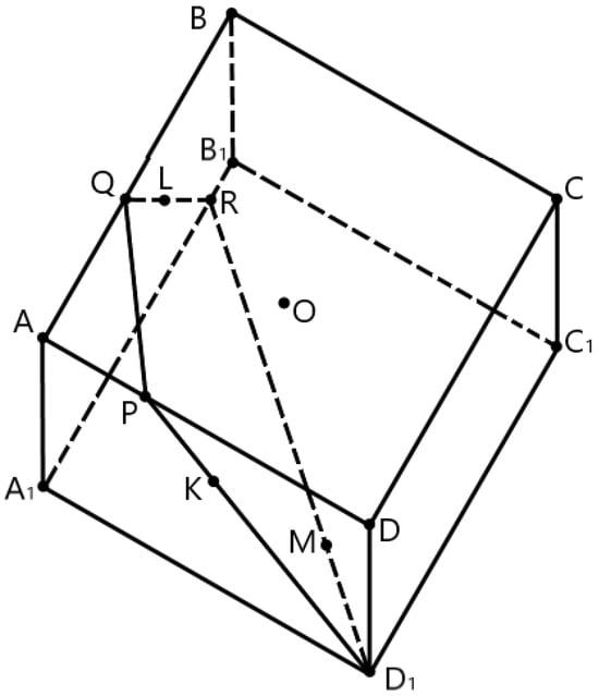
Obviously, the proof must be based on the property of convexity of the set . If the assertion of Lemma 3 for the subset of the set M, which is limited only by the tangency points of the hyperspace by the initial set will be proved, then it will also be proved for the whole set M. Next, consider arbitrary n tangency points of the hyperspace by the set . The hyperplane drawn through these points will always “cut off’’ part of the hyperspace without its center. Thus, no matter what points are chosen, the center of the hyperspace will always be in the “non-cut-off’’ part, and therefore, will be an internal point of the set . Figure 1 shows an illustration for the lemma in space . The statement of the lemma in this case takes the following form: the center of the parallelepiped, inside which there is a convex figure touching each of the sides of the parallelepiped, is an interior point of this figure. As can be seen from the figure, the points of contact of the convex set and M form a plane that “cuts” the initial parallelepiped into two parts, one of which contains its center O. Since the convex set is tangent to each side of the parallelepiped, the point O will always be interior. □

Figure 1.
Illustration for Lemma 3 in space .
3.2. Method for Solving the Efficient System of Inequalities
Details of the efficient system of inequalities solution method are described in this section. Input is a system of double inequalities of the form
This system can also be written as simple linear inequalities:
Thus, the approximation problem has been reduced to a system of linear homogeneous inequalities. For such systems, there are many algorithms for finding a system of generating vectors sufficient to write a general formula for non-negative solutions. However, the resulting system has a special form, significantly different from the general one. In addition, the goal of the approximation problem is not to find all possible solutions to the system. Thus, a fast algorithm for finding a particular solution to the system of inequalities of the obtained form will be described.
The idea of the method is that one or more of the inequalities from (9a)–(9c) can be strengthened using the others. For example, multiplying the inequalities (9a) and (9b) gives:
or
So, the inequality (10), which is a consequence of the inequalities (9a) and (9b), can improve the estimate of the ratio in the inequality (9c). Indeed, if the values are such, that
then the inequality (9c) can be transformed by setting
We use the definition of matrices from the efficient system of inequalities:
If , then, taking into account the ratio (11), the inequality (9c) can be strengthened, setting , as a result of which the set of solutions of the system (9) and the efficient system of inequalities remain unchanged.
Similarly, all the inequalities of the efficient system can be strengthened:
The procedure (12) must be repeated for all possible pairs of jobs . On some steps after the change of it can appear that some of or can also be updated, and the inequality with can be strengthened again, where . Therefore, it is necessary to repeat the procedure (12) until none of the inequalities of the efficient system can be strengthened during the whole iteration. As will be shown in Section 4.3.3, this procedure will need to be repeated not more than times. After that, the values of must also be updated according to the relation (11). The matrices obtained after a sufficient number of repetitions of the procedure (12) will be denoted by .
Thus, if for any pair , then among the inequalities of the system remaining after the corresponding simplifications, there are no pairs that contradict each other. Therefore, for each there exists a solution to the initial system (4) of inequalities such that .
The solution of the system, as shown in Lemma 2, is a convex cone. Therefore, the weight coefficients can be scaled: problems and where are equivalent, and if the set of coefficients is a solution of a system of inequalities (initial or efficient), then the coefficients are also a solution to this system. Due to this fact, one of the weight coefficients can be chosen arbitrarily, then the system can be solved for the remaining weight coefficients, and the resulting solution can be scaled. The resulting solution will correspond to the solution of the initial system of inequalities.
Let, for example, . By Corollary 1 the cross section of the set of solutions of the initial system by the plane is also a convex set. Then, for arbitrary a parallelepiped in a hyperspace of dimension can be described:
Moreover, as was proved above, for all and there exists a solution to the system such that or . In particular, for there exists a solution such that and such that . In other words, the section of the set of solutions by the plane lies inside the parallelepiped described by the inequalities (13) and has at least one common point with each of its faces. Therefore, by Lemma 3 the center of this parallelepiped is an interior point of the set of solutions to the initial system of inequalities and is a solution to the initial system.
The discussion given above can be summarized as the following theorem.
Theorem 1.
A vector , where
is a solution of the efficient system (7) of inequalities (index l can be chosen arbitrarily).
Any value within the interval can be taken as . We used the value in the middle of the interval .
3.3. Algorithm for Solving the Approximation Problem
This section describes the algorithm for solving the problem , with unknown weight coefficients . N instances of this problem are given: , and for each instance the optimal schedule is known. It is necessary to approximate unknown values of the weight coefficients .
The algorithm for approximating the weight coefficients of the objective function is based on solving the efficient system of inequalities:
where:
To approximate the coefficients it is necessary:
4. Numerical Study
4.1. Description of Numerical Experiment
To study the efficiency of the constructed method for approximating the objective function of problem , the solution algorithm described in Section 3.3 was programmed in a Python environment and computational experiments were carried out for various numbers of jobs n and numbers of given instances N with known optimal schedules. For each experiment, weight coefficients and (with a step of 5) problem instances (values and have a uniform distribution on the interval ) were generated, and the constructed approximation algorithm was executed. The algorithm output is a set of the weight coefficients . To compare the found values of and the true weight coefficients , both sets are normalized (scaling is allowed due to the linearity of the objective function):
Measure of efficiency of the algorithm is the modulus of the relative deviation of the found normalized values (averaged over ) from their true normalized values :
The results of a series of experiments for the dependence of the approximation efficiency measure on N for different values of n are shown in Figure 2, Figure 3, Figure 4 and Figure 5.
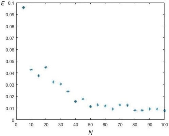
Figure 2.
Modelling results, .
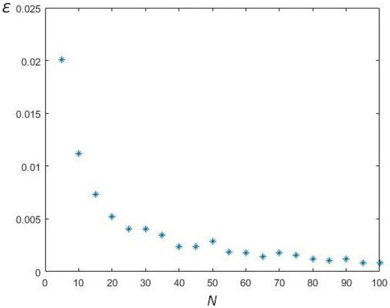
Figure 3.
Modelling results, .
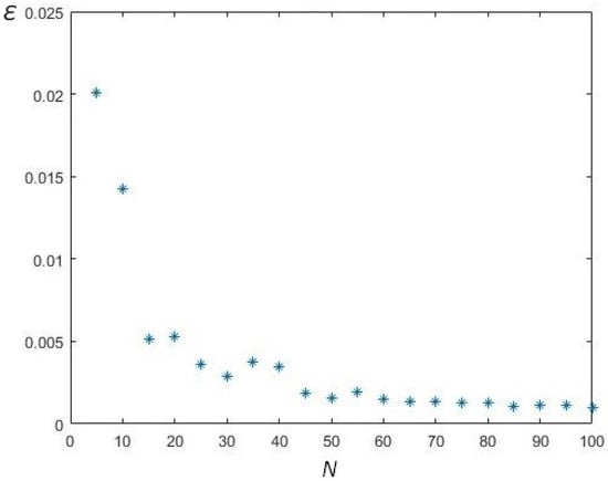
Figure 4.
Modelling results, .
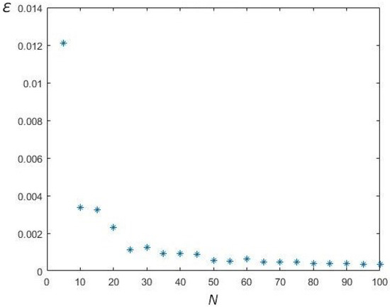
Figure 5.
Modelling results, .
4.2. Analysis of Experiment Results
Function decreases as the number of known optimal schedules N increases. Moreover, the least squares (LSM) approximation of the dependence of on N by the line in all cases with a sufficiently large number of repetitions of the experiment, gives a high linear correlation coefficient . In Figure 6 a graphical representation of the result of a linear approximation with a linear correlation coefficient of is presented.
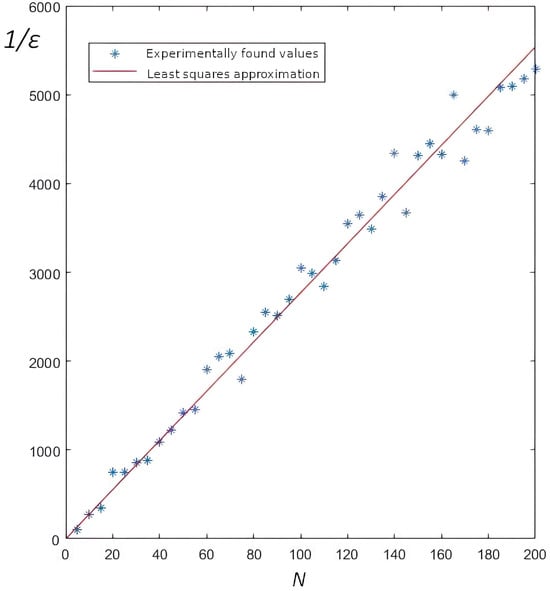
Figure 6.
Modelling results, .
Due to the described correlation, the following hypothesis about the type of dependence is made:
This hypothesis possibly depends on the distribution of the input parameters with the growth of the number n of jobs and number N of given instances with known optimal schedules.
Moreover, as can be seen from the diagrams above, with a greater number of jobs n, more accurate results of the algorithm can be obtained. That is, the function tends to be decreasing. For accurate statistical verification of the hypothesis, it is necessary to conduct a large number of computational experiments.
4.3. Computational Complexity Estimation
The approximation algorithm consists of four sequential procedures:
- construction of sets ;
- calculation of matrices ;
- calculation of matrices ;
- calculation of .
The computational complexity of each of these procedures will be as follows.
4.3.1. Construction of Sets
As it was described in Section 3.1, sets and are defined as follows:
To construct these sets, it is necessary to determine the position of each requirement in each schedule , . Then, for each pair of different jobs it is necessary to compare their positions in schedule . Therefore, the construction of sets requires the following number of operations:
where n is a number of jobs, N is a number of schedules.
4.3.2. Calculation of Matrices
The matrices are calculated as follows:
For each instance of the problem and all possible pairs the ratio is calculated, which requires operations. Then, for each set , the largest value is chosen, which is placed in , which requires operations. After all, finding taking into account the relation (11) requires operations. Therefore, to calculate the matrices , it is required to perform the following number of operations:
4.3.3. Calculation of Matrices
Calculation of the matrices is the most time-consuming part of the algorithm in terms of computational complexity. Indeed, a procedure of the form (12):
for each pair involves computing the product and finding the maximum of values. Thus, the number of operations required to perform the procedure (12) once is
To find the matrices , it is necessary to repeat the procedure (12) in a loop for all possible pairs of jobs until there will be no such pair so that the element can be increased. However, after each repetition of the procedure, the element either is increased or unchanged, so the number of repetitions of the procedure can be significantly reduced. This can be conducted by choosing a special order in which the pairs are considered such that the procedure (12) will be executed for each pair of jobs no more than two times. In this case, the number of operations required to calculate the matrices , is
4.3.4. Calculation of
Computational complexity of finding all values
is operations.
4.3.5. Resulting Complexity
Thus, the computational complexity of the algorithm can be estimated with the following number of operations:
5. Conclusions
The result of the work is an algorithm for approximating the values of the weight coefficients of the problem using N given instances of the problem with known optimal schedules. The result of the algorithm is a set of weight coefficients such that for each of the N given instances, the optimal schedule found for the approximate values of the weights either is equal to the given optimal schedule corresponding to the unknown true set of weights , or has the same objective function value with it. The results described in this paper are also relevant to the problem .
The computational complexity of the algorithm is limited to operations, where n is the number of jobs and N is a number of initial instances with known optimal schedules.
A numerical experiment was carried out to study the efficiency of the method. All shown examples have given instances of the problem , where the number of jobs n is the same for all instances in each set and were given from the interval to check the correlation. The accuracy of the algorithm is estimated by experimentally measuring the function , which is an indicator of the average modulus of the relative deviation of the found values from the true values . An analysis of the results shows a high correlation between the dependence and a function of the form , where is a decreasing function of n. So, based on the result of the experiment, it is clear that a greater number of jobs n, more accurate results of the algorithm can be obtained. In Section 4.2 it is shown that the dependence of on N is approximated by the line ; the least squares method shows a high linear correlation coefficient in all cases with a sufficiently large number of repetitions of the experiment.
Based on the current results, further work is planned in the following areas:
- searching for a formal proof of the hypothesis about the form of dependence from Section 4.2 when ;
- continue studying the general case , where jobs can have different release times; it is necessary to find either a subsystem of inequalities with a polynomial number of inequalities, equivalent to the original system, or the strongest subsystem with a polynomial number of inequalities with an estimate of the approximation error;
- trying to adapt the results to solve the problem of approximating more complex objective functions.
Author Contributions
Conceptualization, A.L.; methodology, A.L. and N.P.; software, E.B.; validation, A.L. and N.P.; formal analysis, A.L. and N.P.; investigation, E.B and N.P.; data curation, E.B.; writing—original draft preparation, E.B. and N.P.; writing—review and editing, A.L. and N.P.; visualization, E.B.; supervision, A.L.; project administration, A.L. All authors have read and agreed to the published version of the manuscript.
Funding
This research received no external funding.
Data Availability Statement
The paper describes a theoretical research. No new data were created or analyzed in this study. Data sharing is not applicable to this article.
Acknowledgments
Authors gratefully thank Nikolay A. Loginov, who took an active part at the initial stage of the work.
Conflicts of Interest
The authors declare no conflicts of interest.
References
- Vahedi-Nouri, B.; Tavakkoli-Moghaddam, R.; Hanzálek, Z.; Dolgui, A. Production scheduling in a reconfigurable manufacturing system benefiting from human-robot collaboration. Int. J. Prod. Res. 2024, 62, 767–783. [Google Scholar] [CrossRef]
- Lazarev, A.A.; Nekrasov, I.; Pravdivets, N. Evaluating typical algorithms of combinatorial optimization to solve continuous-time based scheduling problem. Algorithms 2018, 11, 50. [Google Scholar] [CrossRef]
- Rzevski, G.; Skobelev, P.; Zhilyaev, A. Emergent Intelligence in Smart Ecosystems: Conflicts Resolution by Reaching Consensus in Resource Management. Mathematics 2022, 10, 1923. [Google Scholar] [CrossRef]
- Lei, D.; Liu, M. An artificial bee colony with division for distributed unrelated parallel machine scheduling with preventive maintenance. Comput. Ind. Eng. 2020, 141, 106320. [Google Scholar] [CrossRef]
- Zhao, X.; Liu, H.; Wu, Y.; Qiu, Q. Joint optimization of mission abort and system structure considering dynamic tasks. Reliab. Eng. Syst. Saf. 2023, 234, 109128. [Google Scholar] [CrossRef]
- Koulamas, C.; Kyparisis, G.J. A classification of dynamic programming formulations for offline deterministic single-machine scheduling problems. Eur. J. Oper. Res. 2023, 305, 999–1017. [Google Scholar] [CrossRef]
- Martinelli, R.; Mariano, F.C.M.Q.; Martins, C.B. Single machine scheduling in make to order environments: A systematic review. Comput. Ind. Eng. 2022, 169, 108190. [Google Scholar] [CrossRef]
- Tanaka, K.; Vlach, M. Minimizing maximum absolute lateness and range of lateness under generalized due dates on a single machine. Ann. Oper. Res. 1999, 86, 507–526. [Google Scholar] [CrossRef]
- Mosheiov, G.; Oron, D.; Shabtay, D. Minimizing total late work on a single machine with generalized due-dates. Eur. J. Oper. Res. 2021, 293, 837–846. [Google Scholar] [CrossRef]
- Hermelin, D.; Karhi, S.; Pinedo, M.; Shabtay, D. New algorithms for minimizing the weighted number of tardy jobs on a single machine. Ann. Oper. Res. 2021, 298, 271–287. [Google Scholar] [CrossRef]
- Janiak, A.; Kovalyov, M. Single machine group scheduling with ordered criteria. Ann. Oper. Res. 1995, 57, 191–201. [Google Scholar] [CrossRef]
- Rudek, R. The single machine total weighted completion time scheduling problem with the sum-of-processing time based models: Strongly NP-hard. Appl. Math. Mod. 2017, 50, 314–332. [Google Scholar] [CrossRef]
- Lazarev, A.; Pravdivets, N.; Werner, F. On the dual and inverse problems of scheduling jobs to minimize the maximum penalty. Mathematics 2020, 8, 1131. [Google Scholar] [CrossRef]
- Chernikov, S. Linear Inequalities. In Itogi Nauki i Tekhniki. Series ‘Algebra. Topology. Geometry’; VINITI: Moscow, Russia, 1968. (In Russian) [Google Scholar]
- Chernikova, N.V. Algorithm for finding a general formula for the non-negative solutions of a system of linear inequalities. USSR Comput. Math. Math. Phys. 1965, 5, 228–233. [Google Scholar] [CrossRef]
- Zhu, Y. Generalizations of some fundamental theorems on linear inequalities. Acta Math. Sin. 1966, 16, 25–40. [Google Scholar]
- Fan, K. On infinite systems of linear inequalities. J. Math. Anal. Appl. 1968, 21, 475–478. [Google Scholar] [CrossRef]
- Eckhardt, U. Theorems on the dimension of convex sets. Linear Algebra Appl. 1975, 12, 63–76. [Google Scholar] [CrossRef][Green Version]
- Eckhardt, U. Representation of Convex Sets. In Extremal Methods and Systems Analysis; Springer: New York, NY, USA, 1980. [Google Scholar]
- Lenstra, J.; Rinnooy Kan, A.; Brucker, P. Complexity of Machine Scheduling Problems. Ann. Discret. Math. 1977, 1, 343–362. [Google Scholar]
- Lazarev, A. Scheduling Theory: Methods and Algorithms; ICS RAS: Moscow, Russia, 2019. (In Russian) [Google Scholar]
- Smith, W. Various optimizers for single-stage production. Nav. Res. Logist. Q. 1956, 3, 59–66. [Google Scholar] [CrossRef]
Disclaimer/Publisher’s Note: The statements, opinions and data contained in all publications are solely those of the individual author(s) and contributor(s) and not of MDPI and/or the editor(s). MDPI and/or the editor(s) disclaim responsibility for any injury to people or property resulting from any ideas, methods, instructions or products referred to in the content. |
© 2024 by the authors. Licensee MDPI, Basel, Switzerland. This article is an open access article distributed under the terms and conditions of the Creative Commons Attribution (CC BY) license (https://creativecommons.org/licenses/by/4.0/).