Article

Invariant Feature Learning Based on Causal Inference from Heterogeneous Environments

School of Mathematics, Renmin University of China, Beijing 100872, China
*
Author to whom correspondence should be addressed.
Mathematics 2024, 12(5), 696; https://doi.org/10.3390/math12050696
Submission received: 28 December 2023 / Revised: 22 February 2024 / Accepted: 23 February 2024 / Published: 27 February 2024

Abstract

:
Causality has become a powerful tool for addressing the out-of-distribution (OOD) generalization problem, with the idea of invariant causal features across domains of interest. Most existing methods for learning invariant features are based on optimization, which typically fails to converge to the optimal solution. Therefore, obtaining the variables that cause the target outcome through a causal inference method is a more direct and effective method. This paper presents a new approach for invariant feature learning based on causal inference (IFCI). IFCI detects causal variables unaffected by the environment through the causal inference method. IFCI focuses on partial causal relationships to work efficiently even in the face of high-dimensional data. Our proposed causal inference method can accurately infer causal effects even when the treatment variable has more complex values. Our method can be viewed as a pretreatment of data to filter out variables whose distributions change between different environments, and it can then be combined with any learning method for classification and regression. The result of empirical studies shows that IFCI can detect and filter out environmental variables affected by the environment. After filtering out environmental variables, even a model with a simple structure and common loss function can have strong OOD generalization capability. Furthermore, we provide evidence to show that classifiers utilizing IFCI achieve higher accuracy in classification compared to existing OOD generalization algorithms.

1. Introduction

Traditional machine learning algorithms that rely on independent and identical distribution (i.i.d) hypotheses have been considerably successful. However, they often face challenges in generalization performance when confronted with distribution shifts, a common occurrence in real-world datasets. Specifically, situations arise where training and testing data are drawn from different distributions. Consequently, a machine learning algorithm trained on the training data may struggle to make accurate predictions on the testing data [1]. Thus, ensuring a machine learning algorithm’s capability for out-of-distribution (OOD) generalization and maintaining stable performance under distribution shifts becomes paramount, especially in critical applications such as medical diagnosis, criminal justice, financial analysis, etc. [2].
For classified tasks, traditional machine learning methods that minimize the model’s risk on the entire dataset may struggle to distinguish the true causes of labels from spurious correlations. Consider, for instance, a problem of classifying images of cows and camels [1,3]. As we all know, most cattle are found in grasslands, whereas most camels are found in the desert. This introduces selection bias, causing the trained model to rely on spurious correlations between the environment and the animals. Therefore, after training on this dataset, the model fails to correctly classify simple examples of cow images when they are taken on sandy beaches. In summary, traditional methods based on empirical risk minimization can lead to significant errors when confronted with out-of-distribution data.
In the example above, the background color is an environmental feature that can vary with the sampling environment. In the context of animal classification, features such as shape, color, texture, etc., are the ones that truly establish a causal relationship with the animal category. Advanced deep learning models, such as Convolutional Neural Networks (CNNs), can extract various features from images. However, they cannot distinguish between environmental features and causal features. Other deep learning models encounter similar challenges, as they are primarily designed to learn correlations from observational data rather than capture causality.
It is crucial for the OOD problem to distinguish which features of the data are affected by the environment or exhibit spurious correlations with the target and which features are direct causes of the target [4]. In most out-of-distribution generalization problems, features acting as direct causes of the target variable maintain an invariant joint distribution with the target variable. Therefore, the direct causes of the target variable are often referred to as invariant features. An essential approach involves empowering the model to identify invariant features from the observed data and subsequently use these invariant features to predict the target variable. In this paper, we propose a method of learning invariant features based on causal inference (IFCI) to solve this problem. Our method leverages datasets from multiple environments to infer the features affected by the environments. Firstly, we assume that the data generation process adheres to the following causal mechanism:
y f ( Φ c ( x ) ) e Φ e ( x ) ,
where x and y represent the observational data and labels, respectively; e represents the environment, which can be obtained from a heterogeneous environments dataset; and Φ c ( · ) : X R c and Φ e ( · ) : X R e are the feature extraction processes [1,4]. We refer to Φ c ( x ) and Φ e ( x ) as causal features and environmental features, respectively. Therefore, if the predictor focuses on causal features, it will not be affected by environmental changes. The IFCI model we propose aims to learn the feature extraction process Φ c ( · ) .
In this paper, we extract causal features through causal inference methods and statistical hypothesis testing. However, conducting causal inference and hypothesis testing among all variables requires substantial computational resources, especially when dealing with high-dimensional data. Therefore, according to the data-generating process, we divide the features of observational data z into three modules, namely causal features z c , environmental features z e , and redundant features z r , i.e., z = z c z e z r . The causal graph of our model is illustrated in Figure 1a. We offer a detailed explanation of the definitions of z c , z e , and z r in Definition 2. The modular method [5] helps eliminate redundant causal relationships we do not care about.
In Figure 1a, we can observe the challenges encountered in out-of-distribution prediction: If an algorithm fails to identify environmental features, its classification model might incorporate environmental variables when making category inferences. This is problematic because a correlation between Y and Z e could be a spurious correlation. For the same Y, the distribution of Z e will change after a shift in the environment, so the correlation between Z e and Y will change, which causes the failure of the model trained on the previous environment. Thus, the utilization of environmental features by the predictor is the primary reason for the predictor’s failure on OOD data.
In general, the gold standard for calculating causal effects is through random experiments [6]. For instance, if we aim to investigate whether smoking causes people to develop lung cancer, a randomized experiment would involve identifying two groups of individuals identical in all aspects except for their smoking habits. One group would be designated as smokers (the smoking group), while the other would abstain from smoking (the non-smoking group). Researchers would then assess whether smoking is the cause of the development of lung cancer by observing whether there is a significant difference in the number of individuals developing lung cancer in each group. From the example above, it can be seen that randomized experiments are often impractical and can involve significant costs and ethical concerns in many situations. The model we propose aims to make generalizable predictions using observational data. We leverage causal graphs and adjustment formulas to estimate causal effects from observational data [6,7]. To identify environmental features from observational data across multiple environments, we use E [ z | d o ( e ) ] to evaluate the causal effect of the environment on the features, where d o ( · ) represents the do-operator [6,7]. The interference of potential confounders on the causal effect is mitigated by E [ z | d o ( e ) ] .
The Average Causal Effect (ACE) is usually used to measure the causal effect between treatment variables X and potential outcome Y, and it is expressed in Equation (2) [6,7].
A C E = P ( Y = y | d o ( X = x ) ) P ( Y = y | d o ( X = x ) )
However, when X takes on more than two values, the ACE alone cannot measure the causal effect between variables. Therefore, we introduce statistical methods instead of the ACE to test the association between E [ z | d o ( e ) ] and e. We have demonstrated that by transforming the variable Z, focusing on the mean value E [ z | d o ( e ) ] can effectively measure the causal effect between Z and e.
The main contributions of this paper can be summarized as follows:
  • We incorporate causal inference into a machine learning algorithm to identify invariant features, moving beyond a passive search through optimization.
  • We eliminate redundant causal relationships by modularizing features, which significantly reduces the complexity of causal inference. This modularization makes our causal inference algorithm applicable to complex datasets.
  • We introduce a statistical testing-based method for measuring causal effects, addressing the limitation of the Average Causal Effect (ACE). Our proposed method can handle scenarios where the intervention variable can take multiple values.

2. Related Works

Our work primarily involves a combination of OOD generalization and causal inference.
OOD Generalization: The OOD generalization problem [8,9] has been widely observed in various domains [1,4,10,11,12,13,14,15,16,17]. To address this issue, researchers have proposed various algorithms from different perspectives, such as distributional robust optimization [18,19] and causal inference, which points out that OOD data can be categorized into data with diversity shifts [20] and correlation shifts [19]. In this paper, we focus on the latter.
Meanwhile, several existing works have also leveraged causality to investigate the OOD generalization problem [1,4,17,21,22,23,24,25]. In recent years, exploring the relationship among causality, prediction, and OOD generalization has gained increasing interest, particularly since the seminal work by [26]. Causality-based methods rely on the long-standing assumption that the causal mechanism is invariant across different domains [7]. Some researchers have introduced the concept of stable learning by reweighting data to mitigate the impact of confounders on parameter estimation [23,25,27]. However, most of these methods are optimization-based [1,4]. Such methods aim to learn invariant predictors by designing a loss function and incorporating regularization terms within it. Consequently, optimization-based methods aim to extract causal features and make predictions simultaneously by defining specific optimization objectives. Since they do not explicitly identify causal features, these methods often face challenges in demonstrating their ability to effectively extract causal features. Additionally, specific optimization-based methods have been subject to theoretical and experimental studies [28,29], revealing that they frequently fall short of achieving desirable out-of-distribution generalization performance and have stringent requirements on environmental conditions. In this paper, we utilize causal inference to actively search for causal features.
Causal Inference: In many applications, inferring cause–effect relationships between variables is a fundamental objective. This type of causal inference has its roots in diverse fields, with various conceptual frameworks contributing to its understanding and quantification. Among these are the frameworks of potential outcomes and counterfactuals [30,31], structural equation modeling [6,32,33], and graphical modeling [34,35]. Ref. [36] established a connection between these frameworks using single-world intervention graphs. Overviews of different branches of causal inference and their applications in various fields were provided by [37,38]. Summaries of the development and application methods of causal inference in machine learning were presented in [39,40]. Our work uses structural equation modeling to capture the causality of latent variables and the environment.

3. Invariant Feature Detection Based on Causal Inference

In this section, we discuss a method for learning invariant features based on causal inference (IFCI). In Section 3.1, we establish the problem and assumptions. In Section 3.1, we introduce the causal structure behind the prediction problem. In Section 3.3, we present the causal inference method employed in our algorithm.

3.1. Setup and Assumptions

Following [1,2,4], we consider a dataset D = { X e , Y e } e ε a l l from multiple environments and an observed dataset D e = { x i e , y i e } i   =   1 n e , x i X , y i Y and e ε t r , where ε a l l represents all environments and ε t r denotes the set of training environments. The goal of this work is to find a predictor f ( · ) : X Y with good performance on data from all environments [1,2,4,10]. Inspired by [26], we attempt to achieve this goal using causal inference methods. However, conducting causal inference directly from high-dimensional observational data is sometimes impractical, such as inferring the causal relationship between each pixel and class in image classification. Therefore, we define a feature extraction function: Φ : X Z , d i m ( Z ) d i m ( X ) . Then, we infer causal relationships from the obtained high-dimensional features Z. In this section, we assume that reasonable features Z have been extracted. The details of the feature extraction function are introduced in the following section.
In disentangled representation learning tasks, the goal is to learn independent representations to enhance the model’s performance [41,42]. However, achieving fully independent representations is often challenging. Our method does not require completely independent data representations. Therefore, we employ a modular approach [5] to eliminate redundant causal relationships.
 Definition 1.
A subset of latent features I is termed modular whenever Z is the Cartesian product of Z I  and  Z I ¯ .
Our method only makes a weaker assumption about the independence among modules. We divide the latent feature Z into three parts: Z c , Z e , and Z r . Then, in Assumption 1, we impose restrictions on the causal directions among modules. Assumption 1 indicates that Z c is not the parent node of Z e in the causal graph, but Z c can still influence Z e through Y.
 Assumption 1.
The causal features Z c are not a direct cause of the environmental features Z e .
Assumption 1 can be seen as a relaxed version of the disentangled representation in which independent representations are required. It requires that the causal features of the target variable are not direct causes of environmental features. Therefore, this assumption is easier to achieve through feature extraction models.
Without any prior knowledge or causal structural assumptions, it is impossible to figure out the OOD generalization problem since one cannot characterize the unseen latent environments in ε a l l . A commonly used assumption in the invariant learning problem was proposed in [1,2,43]:
Assumption 2.
There exists a random variable Φ c X such that the following properties hold:
(a) 
Invariance property: for all e , e ε a l l , we have that P e Y | Φ c X = P e Y | Φ c X holds.
(b) 
Sufficiency property: Y = f Φ c X , ϵ , ϵ X .
This assumption indicates the existence of invariant features and their sufficiency for predicting the target Y using Φ c . The sufficiency property coincides with the causal mechanism we proposed in (1).
According to the second equation in Equation (1), Z e changes with the environment e. Therefore, a predictor that depends on the environmental features may fail in a new environment. Our proposed method utilizes the dependence of environmental features on the environment to identify them.
 Assumption 3.
For any X E n v i r o n m e n t e , Z = Φ X N ( μ , ) . Following the data-generation process (1), Z e is generated from P Z e | e . There exist at least two environments e 1 , e 2 ε t r such that P e 1 Z e P e 2 Z e .
Assumption 3 imposes a constraint on the training dataset. This assumption indicates that the causal relationship between the environment and its features varies with environmental changes.

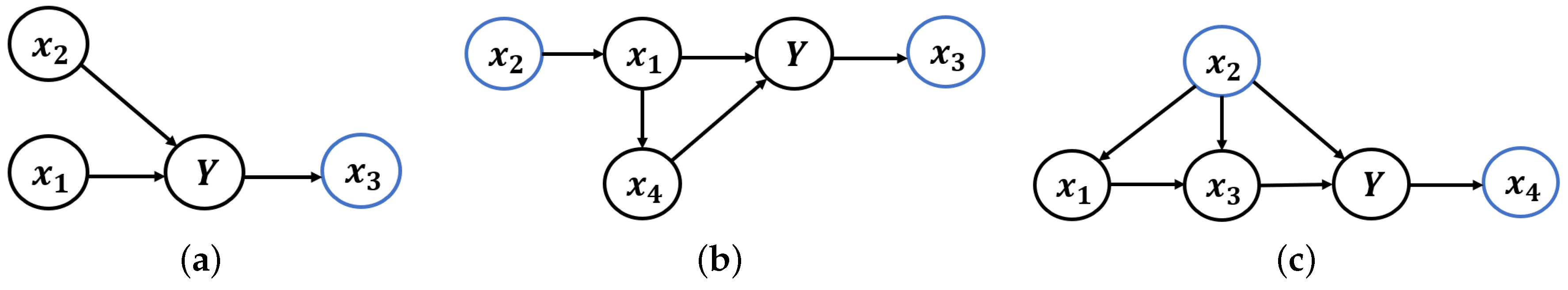
3.2. Causal Structure behind the Predict Problem

Numerous variables exist in the observational data, resulting in a complex causal relationship between variables even after feature extraction. Consequently, making causal inferences at the variable level becomes impractical. We divide feature vector Z into three modules according to the causal relationship among features Z, target Y, and environment e. The three modules are defined as follows:
 Definition 2.
(a) 
If a variable Z i is the cause of Y, then Z i is called a causal variable. All causal variables constitute the causal features.
(b) 
If a variable Z i is not the cause of Y and the environment e is the cause of Z i , then Z i is called an environmental variable. All environmental variables constitute the environmental features.
(c) 
If a variable Z i is in the latent features but Z i is not the causal variable or environmental variable, then Z i is called a redundant variable. All redundant variables constitute the redundant features.
Given that our objective is to discern environmental features Z e from Z by estimating causal effects, this modular method preserves the relevant causal relationships while eliminating the redundant ones.
 Proposition 1.
Under Assumption 2, Z e and e are not the cause of Z c or Y.
The proof of Proposition 1 is detailed in Appendix A. Building on Assumption 1 and Proposition 1, we construct the causal graph (Figure 1a), depicting the causal relationships between the modules and targets. The dynamic distribution of the environmental variable Z e across different environments poses a challenge for traditional empirical risk minimization (ERM) methods, which utilize all input features to generalize effectively out of the distribution. Consequently, our method seeks to sift out the descendants of the environmental variables (nodes directly or indirectly influenced by the environmental variable e in the causal graph) among the feature variables through causal inference.
The introduction of the modular method facilitates straightforward causal inference on high-dimensional features, as depicted in Figure 1a. The causal graphs we encounter may exhibit much greater complexity when analyzed from a non-modular perspective, as illustrated in Figure 1b. In Figure 1b, we use environmental features Z e as an example to illustrate the complex causal relationships that may exist within modules. For simplicity, we do not show the internal causal relationships between causal features Z c and redundant features Z r , as in reality, they may also have complex causal graphs internally. Given that variables within modules can have causal relationships, the number of tests required when the variables increase in the non-modularized approach grows exponentially. Specifically, if the number of variables is d, the number of tests is O ( 2 d ) . However, with our modularized method, since we only need to test the causal relationships among features, labels, and environmental variables, the number of tests maintains a linear relationship with the number of variables, i.e., the number of tests is O ( d ) . Consequently, the modularized approach significantly mitigates the complexity of causal inference. In the next section, we also demonstrate through experiments that our method exhibits rapid convergence speed.
In Figure 1, the black arrows are derived from the definitions of Z c and Z e . The blue arrows are established based on Assumption 1. Two causal paths exist from e to Z e : e Z e and e Y Z e . The second path represents the backdoor path from e to Z e . Therefore, according to the backdoor criterion, we can compute P Z = z | d o e from the observational data as follows:
P Z = z | d o e = y P Z = z | e , Y = y P Y = y .
We mitigate the impact of the confounder Y on the estimation of the causal effect between e and Z by employing Equation (3). We introduce the backdoor criterion in Appendix B.

3.3. Causal Inference with Multiple Environments

In this section, we use multi-environment data to infer the environmental features Z e . Subsequently, we introduce an OOD prediction algorithm by making predictions using features other than environmental features.

3.3.1. The Mean after Intervention

As discussed in Section 1, we introduce a novel causal estimation method to estimate the causal effect, replacing the ACE. Traditional methods, such as the adjustment formula (Equation (3)) or inverse probability weighting, are commonly employed for inferring causality from correlations [6]. However, both approaches necessitate the estimation of the probability distribution after intervention. Given that the latent variable Z is a continuous random vector, estimating the probability distribution after intervention becomes challenging. To address this, we propose a mean-based statistical testing method to assess the causal effect.
 Theorem 1.
Under Assumption 3, let z e i , j denote the jth dimension of z in the ith environment, z e i , j N ( μ e i , j , σ e i , j 2 ) . If μ ˜ e 1 , j = μ ˜ e 2 , j = · · · = μ ˜ e i , j , where μ ˜ e i , j = μ e i , j σ e i , j , the distribution of z e i , j remains constant for all e i .
The proof of Theorem 1 is provided in Appendix A. From the proof of Theorem 1, it becomes evident that we normalize z as z ˜ , where its mean is μ ˜ = μ σ . After normalization, the variance differences between different environments are translated into differences in the mean values. According to Theorem 1, the mean value after intervention is the only statistic of concern.
 Proposition 2.
Following (3), we can obtain the mean after intervention:
E Z = z | d o e = y P Y = y E Z e | Y = y , e
The proof of Proposition 2 is shown in Appendix A. Our method first calculates the mean of feature z after intervening in environment e using Equation (4), which we denote as μ . Then, applying the formula for variance D ( X ) = E ( X 2 ) E ( X ) 2 , we derive the variance after intervention σ 2 . This allows us to compute μ ˜ = μ σ , as discussed in Theorem 1. After obtaining the probability distribution after intervention, we use hypothesis testing for variables that have significant causal effects with the environment e.

3.3.2. Analysis of Variance in Causal Inference

The distribution of environmental variables changes with the environment. Therefore, we aim to identify which variables in Z exhibit significant differences across different environments. In our method, we employ analysis of variance (ANOVA) [44] to test the significance of the differences among variables in various environments. Additional details about the introduction of ANOVA and the abbreviations used in ANOVA can be found in Appendix C.
In Section 3.3.1 and Appendix A, we have demonstrated that z j exhibits the same variance. Therefore, z j aligns with the assumption that the dependent variables in each category share the same variance. Our method utilizes the mean value after intervention to compute the SSA and SSE (the descriptions of the SSA, SSE, and x ¯ ¯ are shown in Appendix C). Subsequently, we calculate the total mean value x ¯ ¯ , and the SSA, SSE, and F-statistic using the method outlined in Appendix C. We adopt a significance level α of 0.05.
Using ANOVA, we identify the dimensions in Z whose mean value is not influenced by the environment. Subsequently, the variance difference of Z in each environment is transformed into a difference in the mean value through normalization. Therefore, based on Assumption 3, the distribution of the screened variables is not affected by the environment. The algorithm for filtering environmental variables through causal inference is summarized in Algorithm 1.
Through Algorithm 1, we obtain the indices of environmental variables Z e , allowing us to remove these dimensions in the downstream tasks while retaining Z c and Z r . Redundant variables Z r are not contributory to prediction; however, their distributions are independent of the environment, ensuring no spurious correlations between redundant variables Z r and prediction variables Y. Therefore, in classification, clustering, or regression tasks, the optimization algorithm, such as gradient descent, minimizes the parameters of Z r . Thanks to the modular approach, we only need to test the causal effect between the feature Z and the environment, resulting in a final computational complexity of O ( d ) . In contrast, without the use of a modularized causal inference method, it would be necessary to calculate the causal effects between all variables, leading to a computational complexity of O ( 2 d ) , which is often infeasible for high-dimensional data.
Algorithm 1 Filter environmental variables
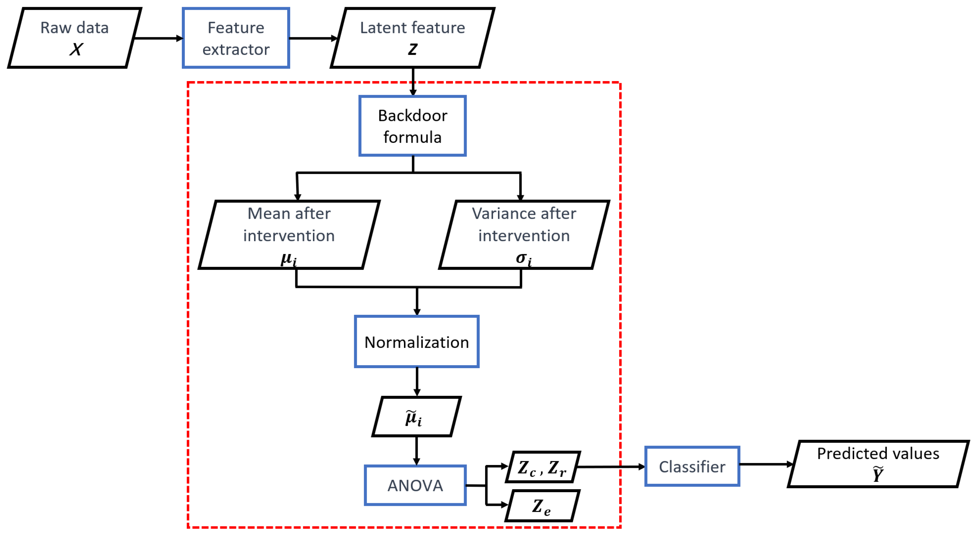
 Z e
Input:  z i 1 , y i 1 , z i 2 , y i 2 , · · · , z i n i , y i n i , i = 1 , 2 , · · · , k , z i j R d , y i j N + , e i N + , α .
Output: The indices of environmental variables  I n d e x = i n d e x 1 , i n d e x 2 , .
 1:  I n d e x =  
 2: for  i n d = 0 to l e n g t h z  do
 3:  Calculate the mean value and the variance after intervention:
     μ i = y P y E z i n d | y , e ( z i denotes the ith dimension of z),
     σ i = μ i ( z 2 ) μ i 2
 4:  Normalization: μ ˜ i = μ i σ i
 5:  Construction of test statistics: z ¯ ¯ = i = 1 k n i μ ˜ i n , S S A = i = 1 k n i μ ˜ i z ¯ ¯ 2 ,
     S S E = i = 1 k j = 1 n i z i j μ ˜ i 2
 6:  Calculate F statistics: F = S S A k 1 S S E n k
 7:  if  F > F α  then
 8:    I n d e x i n d
 9:  end if
 10: end for
 11:
 12: return  I n d e x
Figure 2 illustrates the system architecture of our algorithm. Here, μ i represents the mean of feature Z i after intervening in environment e, and σ i represents the variance of feature Z i after intervening in environment e.

4. Empirical Studies

In this section, we assess the effectiveness of the proposed IFCI algorithm using simulated data, semi-synthetic data, and real-world data. We trained the model on data from certain available domains and evaluated its performance on data from the remaining domains not used during training. The code for the IFCI algorithm can be downloaded from https://github.com/hangsuuuu/IFCI (accessed on 10 January 2024). To further evaluate the value of the IFCI algorithm, we utilized current mainstream causal invariant learning methods in our experiment: ICP [26], IRM [1], V-REx [45], RVP [46], and CoCo [4]. Among them, IRM, V-REx, RVP, and CoCo are based on regularized optimization of invariant learning algorithms, and RVP and CoCo are the latest causal invariant learning algorithms. ICP is a classic method that utilizes hypothesis testing for causal inference. In addition, to evaluate whether there was a difference in data distribution between the training dataset and the testing dataset, we used an empirical risk minimization (ERM)-based model as a benchmark. We can evaluate whether an algorithm has out-of-distribution generalization ability by comparing it with the ERM model.

4.1. Linear Simulated Data

In this section, we initially assess the performance of IFCI on linear simulated data. We generated data from three distinct causal graphs, individually evaluating the performance of IFCI in each of these scenarios. The causal graphs for the three datasets are presented in Figure 3, and the data-generation formulas are explained in detail in Appendix F.
The relationships between variables followed a linear mapping with additive noise. To generate data from different environments, we set the parameter γ e 0.5 , 1.0 , 5.0 (for the usage of γ e , please refer to Appendix F). We generated 10,000 data points for the first and third environments and 3000 data points for the second environment. In this experiment, we simulated selection bias that might occur during data collection by generating varying amounts of data in different environments—the first two as training environments and the last one as a testing environment.
These three cases corresponded to the different causal graphs. We used this example to test the performance of IFCI when the data partially violated the assumption. IFCI uses a linear layer to process features, followed by mapping the output values to the [0, 1] range through the sigmoid function. We compared IFCI with the following methods: ERM, Invariant Causal Prediction (ICP) [26], Invariant Risk Minimization (IRM) [1], Risk Extrapolation (V-REx) [45], Risk Variance Penalization (RVP) [46], and Constrained Causal Optimization (CoCo) [4]. RVP and CoCo are the most recent optimization-based methods for invariant learning. ICP is a classic method that utilizes hypothesis testing for causal inference. All the parameter settings and training configurations for the models involved in the comparison are described in Appendix E. The experimental results are presented in Table 1, Table 2 and Table 3.
Table 1, Table 2 and Table 3 show that ERM exhibited a significant difference between the testing and training accuracies. This is because the selection bias in the data led ERM to rely on environmental variables. The optimization-based causal learning methods (IRM, V-REx, RVP, CoCo) exhibited a somewhat smaller difference between the testing and training accuracies. However, in some cases, such as Case 2 and Case 3, their testing accuracies did not show significant improvements compared to ERM. In Case 2, V-REx and RVP exhibited lower testing accuracies compared to ERM, and their convergence was slower than ERM. This might be due to the variance of the ancestral nodes of the predicted target Y being influenced by the environment, as the performance of V-REx and RVP heavily relied on the assumption of distributional invariance. CoCo typically exhibited a smaller difference between the testing and training accuracies compared to IRM, V-REx, and RVP. However, in Case 3, CoCo performed poorly, with the lowest training and testing accuracies. This may have been due to the strong regularization imposed by CoCo, which weakened the fitting capability of a model with only a single-layer linear structure. Regularization tended to favor simpler model structures during optimization, while overly strong regularization could have made the model too simple and lacking sufficient fitting ability, making it unable to capture the relationships between variables in Case 3. This can be seen in the low accuracy rate of CoCo’s training. IFCI and ICP initially performed feature selection and then used the selected features for prediction. ICP tended to have high variance in its prediction results. In Case 1, ICP correctly identified invariant features, leading to high training and testing accuracies. Since IFCI and ICP use the same predictor, their training results were identical as long as they selected the same features. The difference in convergence time was mainly due to the varying time required for feature selection. ICP needed to test all feature combinations to determine the final set of invariant features, whereas IFCI only needed to test each feature once, making IFCI converge faster than ICP. ICP’s results were empty in Case 2 because ICP rejected the null hypothesis for all feature combinations in this case. In other words, based on its tests, none of the feature sets were considered invariant. As a result, ICP could not train a predictor in Case 2. In Case 3, ICP identified the set of all variables as invariant, so the results of ICP are the same as those of ERM. The failure of ICP in Case 2 and Case 3 is because the environment influenced the parent nodes of the direct causal variables of Y. Although Case 2 and Case 3 violated Assumption 1, the experimental results showed that IFCI performed well in all three cases. This suggests that Assumption 1 is a sufficient condition for Theorem 1 to hold, rather than a necessary condition. IFCI achieved the highest testing accuracy in each case, with a minimal difference between the testing and training accuracies.

4.2. Gaussian Mixture Model
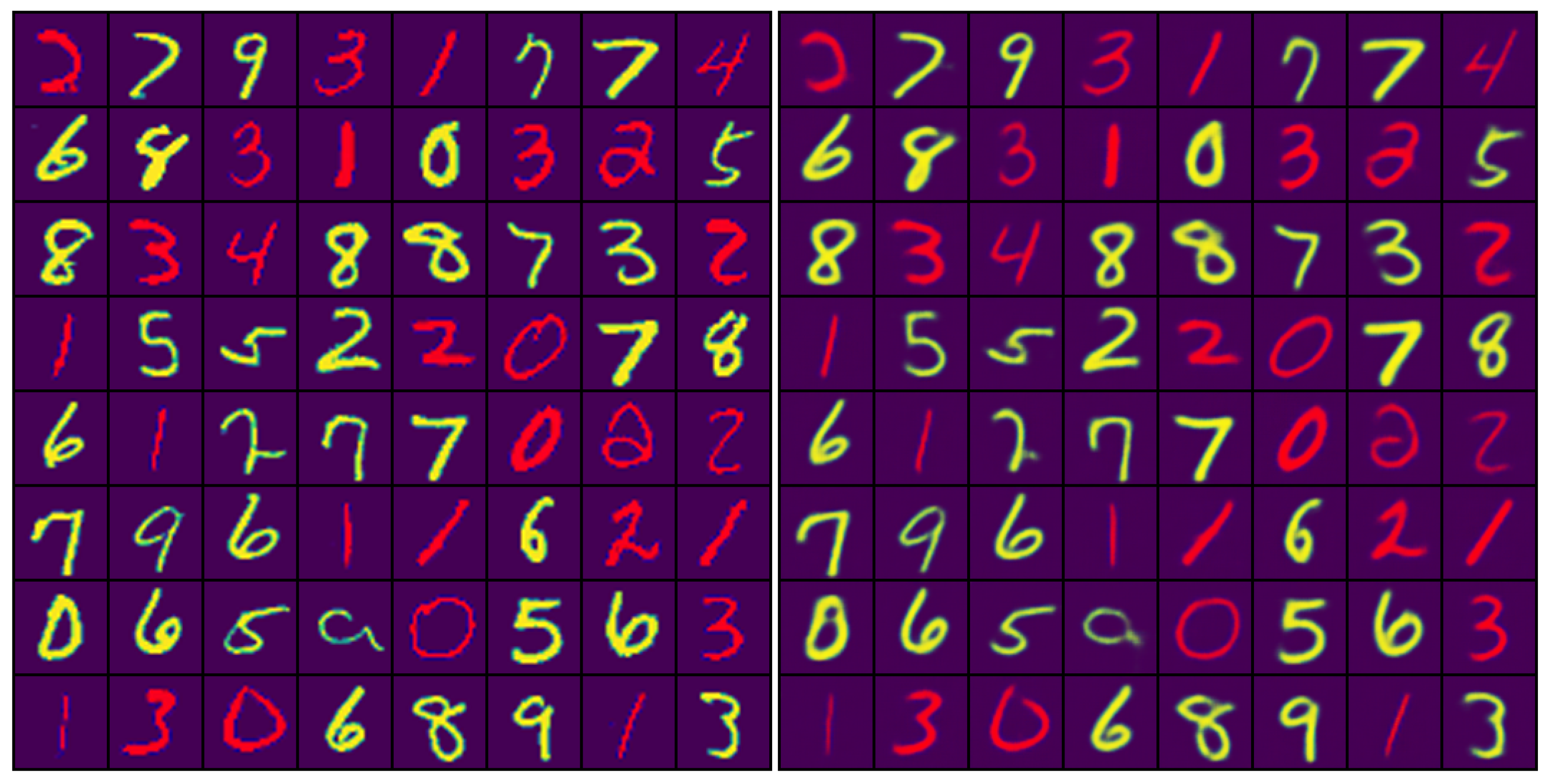
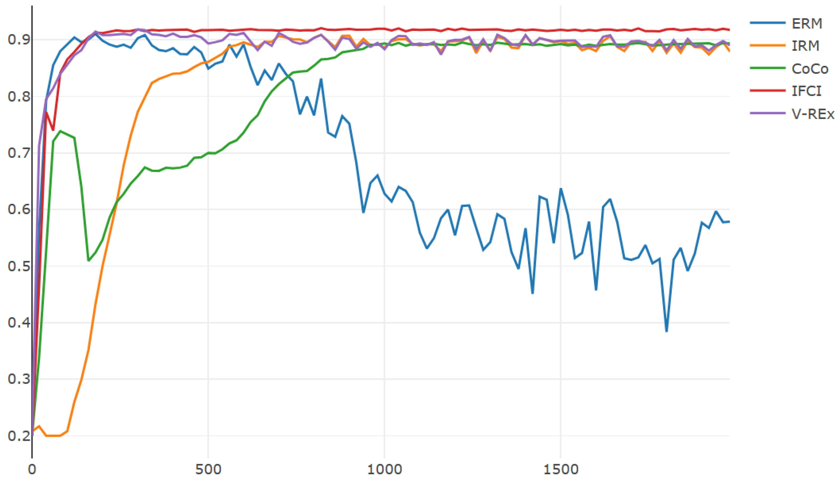
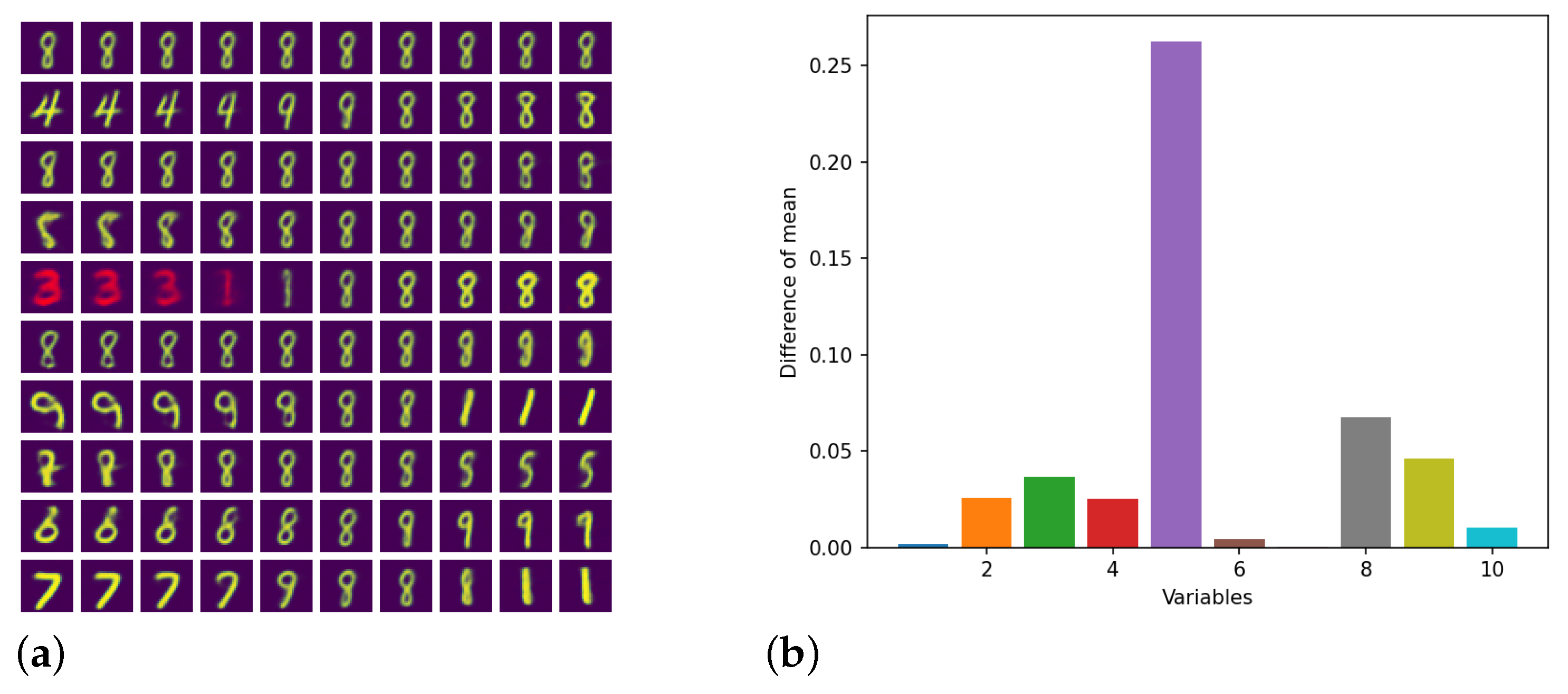
In this subsection, we simulate a Gaussian mixture dataset with a Gaussian mixture model (GMM). We test our algorithm through multi-class classification problems in this example when the inputs contain non-causal covariates [4]. In this dataset, x e , z e are the observed variables and y e is the label associated with the observed variables, where e is the environment index. For environment e, the data are generated using Equation (5):
x e k = 1 K 1 K N μ k , I y e C a t e g o r i c a l p 1 , , p K z e 1 p e δ u y e e + p e δ u k 1 e ,
where p k = N x e ; μ k , I / k = 1 K N x e ; μ k , I , p e depends on environment e, and k 1 M u l t i n o m i a l 1 / K , , 1 / K , corresponding to k 1 = 1 , 2 , , K , respectively. In this model, the distribution of x e and the mapping from x e to label y e are invariant across all e, whereas the distribution of z e depends on e.
The generated data for this example can be obtained from the code available at https://github.com/mingzhang-yin/CoCo (accessed on 1 February 2021). For a detailed explanation of the generation process, please refer to [4].
We generated training environments with K = 5 , where x e has five dimensions, and z e has three dimensions. In this experiment, five different environments were created, each corresponding to p e 0.01 , 0.02 , , 0.05 . In Equation (5), x e is generated by the GMM model with a mean vector μ k = 1.5 K e k R K , where e k is a k-dimensional vector with elements equal to 1. y e is the class corresponding to the maximum value among p k . To generate the environmental variable z e , K random vectors u k t k = 1 K were generated, where u k t i = 1 k 2 U ( 0 , 1 ) for environment e. Since the values of y e and k 1 are in the range 1 , 2 , · · · , K , z e is influenced jointly by y e , k 1 , and p e . Therefore, there is a spurious correlation between z e and y e , but z e is not a causal variable for y e . Additionally, since p e is influenced by the environment, z e is an environmental variable. We set the maximum iterations to 2000. In this example, we used the cross-entropy loss function for IFCI, which is the same as ERM.
We first applied IFCI to the training data to obtain the indices of the invariant features. Subsequently, we configured the predictor as a fully connected neural network with two hidden layers, using only the invariant features as input to the predictor. We evaluated the test performance based on the classification accuracy and convergence time of the models. The parameter settings for ERM, IRM, V-REx, RVP, and CoCo in this experiment are provided in Appendix E.
The results are presented in Figure 4 and Table 4. Figure 4 illustrates the trace plots of the predictive accuracy.
Figure 4 indicates a pattern where the testing accuracy initially increased for all methods during the early stages of training but experienced a decline in the later stages for ERM, IRM, and V-REx. This suggests that ERM, IRM, and V-REx initially enhanced prediction accuracy by leveraging all features, including causal ones. However, in the later training stage, they may have become more reliant on spurious associations, leading to a drop in performance in the test environment. The results of CoCo were relatively unstable, during both training and testing. At times, the accuracy of CoCo even approached that of ERM. This instability could be attributed to CoCo’s sensitivity to variable initialization during training. In contrast, IFCI relied on statistical hypothesis testing for variable selection, making it less sensitive to variations in variable initialization. By successfully identifying environmental variables through causal inference methods and excluding them in the predictor, IFCI rapidly improved the testing accuracy to a high level during training. Ultimately, IFCI converged to the highest testing accuracy at the fastest speed.
Table 4 provides a comprehensive overview of the numerical results obtained in this experiment. Table 4 shows that ERM achieved the highest training accuracy, but its performance on the test set was poor. This discrepancy arose from ERM fitting all features during training, resulting in overfitting. RVP, an enhanced model based on V-REx, generally outperformed V-REx in most cases. However, due to the more intricate calculation of the penalty terms in RVP, it exhibited a slower convergence rate compared to V-REx. Since ICP obtained an empty set as an invariant set in this experiment, it was impossible to train the predictor. Therefore, there are no results corresponding to ICP in Table 4. IFCI exhibited the highest prediction accuracy during testing. Furthermore, IFCI exhibited a minimal difference between the testing and training accuracies, second only to CoCo. Although CoCo’s results fluctuated considerably, there was always a slight difference between the training and testing accuracies of the model trained by CoCo. This was perhaps due to CoCo’s strong focus on invariance during training, which led to a loss of the model’s predictive capability. The IFCI model has fewer parameters than others because it is trained solely on invariant features. As a result, the convergence speed can be even faster than the simplest structured ERM model. Based on optimization, methods like IRM and CoCo exhibited the slowest convergence speeds due to the need for additional gradient computations and more complex loss functions. While IFCI required an additional causal inference stage, our modular approach and simplified hypothesis testing methods significantly reduced the time consumed for causal inference. Moreover, causal inference was performed only once during training, eliminating its need in every iteration. Therefore, IFCI exhibited the fastest convergence speed among all the compared models.
Table 5 summarizes the F-statistics for each dimension in IFCI. Table 5 indicates a significant difference in the F-statistics between causal and environmental variables. In this experiment, the F-value corresponding to a significance level of α = 0.05 was denoted as F 0.05 = 2.37 , allowing for accurate discrimination between environmental variables and causal variables with 100 % accuracy. This underscores the effectiveness of IFCI in practically and reliably separating environmental variables. It is important to note that since other models involved in the comparison did not necessitate the construction of test statistics, Table 5 exclusively includes the F-statistics generated by IFCI.

4.3. Colored MNIST

In this subsection, IFCI is tested on a semi-synthetic dataset known as Colored MNIST [1], designed for binary classification. The Colored MNIST dataset is derived from the MNIST dataset, where handwritten digits 0–4 are labeled as y = 0 and digits 5–9 are labeled as y = 1 . The digits are colored green with a probability of p e when y = 1 and with a probability of 1 p e when y = 0 . If the digit is not colored green, it is colored red. The probability p e of coloring varies across different environments. In this example, training environments were constructed with p e 0.1 , 0.3 , whereas p e = 0.9 was used for testing. The data for this example can be generated using the code available at https://github.com/facebookresearch/InvariantRiskMinimization (accessed on 1 January 2024).
Performing causal inferences on each pixel of the original image data is not meaningful. Therefore, feature extraction becomes essential. In this paper, we chose β -VAE [47] as the feature extractor. VAE [48] is an unsupervised probabilistic model based on variational inference. The VAE model’s structure is illustrated in Figure A1, and the loss function is provided in Appendix D. VAE first maps high-dimensional data to a low-dimensional normal distribution and then resamples from the normal distribution to reconstruct the original image through a decoder. This ensures that the low-dimensional vector obtained through VAE follows a normal distribution using the reparameterization method, ensuring that the features extracted by VAE satisfy Assumption 3. Therefore, theoretically, using VAE guarantees that our model can discover the causal variables. For β -VAE, a hyperparameter β is introduced to the second term of the VAE loss function to enhance the ability to learn disentangled representations.
In this experiment, a four-layer convolutional neural network was employed as the encoder, and a four-layer deconvolution neural network served as the decoder. The hyperparameter β was set to 2, and the dimensions of the latent variables were 10. The reconstructed images from β -VAE are depicted in Figure A2, demonstrating that β -VAE effectively reconstructed the images, signifying that its latent vector Z retained a substantial amount of information from the original images. IFCI was then applied to the low-dimensional vectors extracted by β -VAE to identify the environmental variables. Figure 5 illustrates the interpolation of latent features extracted by β -VAE and the results on the latent variables obtained by IFCI. Since there were only two training environments in this experiment, we compared the difference between the mean values of the two environments to reduce computational complexity.
From Figure 5a, it is evident that the fifth dimension of the latent vector captured the color information of the digits, which is environment-dependent. Consistently, the results obtained by IFCI highlight the fifth dimension with a significantly larger value compared to other dimensions. Therefore, the output of IFCI aligns with the expected outcome, indicating that IFCI successfully identified and emphasized the environment-dependent feature in the latent space.
After filtering out the environmental variables, we input the latent vector into a classifier for classification. In this experiment, we used a fully connected network with three hidden layers as a classifier and employed the binary cross-entropy loss function for IFCI, which was the same as ERM. Table 6 presents the classification accuracies and training times of IFCI, ERM, IRM, V-REx, RVP, CoCo, and ICP. The parameter settings for the comparison models are detailed in [4], and additional parameter settings for the other models are provided in Appendix E.3. Although ERM and V-REx converged quickly, their performance on the test set was even worse than random guessing, indicating a failure to learn invariant features. V-REx and RVP exhibited a significant difference between the training and testing accuracies, indicating that they did not effectively learn the invariant features and were heavily reliant on color features. ICP performed similarly on both the training and testing sets. However, based on the training accuracy, it appears that ICP did not identify all the invariant features but only a subset. Consequently, the model failed to achieve satisfactory predictive performance due to the insufficient features provided to the predictor. Because ICP directly tested the set of invariant features, whereas IFCI tested the environmental features and removed them, the set obtained by ICP was typically a subset of the true set of invariant features. In contrast, the feature set obtained by IFCI included the true set of invariant features. Therefore, IFCI’s set contained more information. Consequently, the training and testing accuracies of IFCI were higher than those of ICP. IFCI requires using β -VAE for feature extraction on image data, so it exhibited a slightly slower convergence speed compared to ERM and V-REx. However, IFCI achieved the highest test accuracy among all the models. This can be attributed to its ability to discover environmental variables that interfered with model generalization and effectively remove them.

4.4. Real-World Data

In this subsection, we utilize the Non-I.I.D. Image Dataset with Contexts (NICO) [49], which contains wildlife and vehicle images captured in different environments. This dataset can be downloaded from https://nico.thumedialab.com (accessed on 18 April 2022). The objective of this example is to classify bears and cows in images. During training, we employed images taken in forests or rivers. During testing, we selected images captured in the snow. Data collected in different environments typically follow distinct distributions due to various physical factors, such as landscape, background color, illumination conditions, etc. These physical factors, reflected in the image background, might be predictive of the species but in a spurious manner.
In this example, we aimed to filter out these factors through IFCI, retaining consistent features across different environments. Similar to the previous example, we utilized the β -VAE model to extract low-dimensional features from images. We employed ResNet18 [50] as the encoder to extract features from real-world images. The reconstructed image of the β -VAE model is illustrated in Figure A3, indicating that β -VAE successfully extracted most of the information from the original image. Subsequently, a five-layer fully connected network was employed for classification. Similar to the previous section, IFCI and ERM used the binary cross-entropy loss function. The parameter settings for the other models are introduced in Appendix E.4. The training accuracy, testing accuracy, and time taken for each model to converge during training are summarized in Table 7.
IFCI still achieved the highest testing accuracy, with a minimal difference between the testing and training accuracies, Although CoCo and ICP also exhibited minimal differences between the testing and training accuracies, their performance was below that of IFCI. This was primarily due to the strong regularization imposed by CoCo and the fact that ICP identified a subset of the true invariant set of features. ERM and V-REx failed in this example because they received interference from spurious correlations, such as environmental backgrounds. The accuracy of RVP was slightly higher than that of V-REx, but there was still a significant difference between its performance on the testing set and the training set. IFCI maintained a relatively fast convergence speed (second only to ERM), so IFCI maintained high prediction accuracy and convergence speed even on larger images.

5. Conclusions and Future Work

In this paper, we present an innovative approach to invariant feature learning called invariant feature learning based on causal inference (IFCI). Our method introduces causal inference into representation learning, enabling machine learning algorithms to acquire causal representations. Through experiments, we validate that algorithms relying on causal representations often exhibit robust generalization capabilities. To facilitate causal inference in high-dimensional data, we adopt a modular approach, which aids in eliminating redundant causal relationships and retaining only those causally linked to the task at hand. For causal inference, we extend the Average Causal Effect (ACE) to handle multiple variable values, facilitating the effective measurement of causal effects. Experimental results demonstrate that IFCI can successfully filter out environmental variables, significantly improving the model’s generalization ability. In summary, our proposed IFCI method addresses the limitations of optimization-based approaches by conducting causal inference at the feature level, thereby enhancing out-of-distribution generalization. Furthermore, the modular approach contributes to faster convergence compared to other methods for out-of-distribution generalization.
In addition to classification, IFCI can also be applied to other problems, such as regression analysis. After filtering environmental variables through IFCI, the regression model can also have a stronger generalization ability. Therefore, the modular methods and construction of causal diagrams in other machine learning problems are worth studying in the future.
A suitable feature extraction method can extract more valuable features. The current feature extraction method we are using is based on unsupervised techniques. However, designing a feature extraction method that effectively utilizes environmental and label information could significantly enhance the model’s performance. Therefore, this will be a direction worth exploring in future research. When designing such a feature extraction method, it is essential to be cautious and avoid being influenced by spurious correlations in the data.
Studying causal learning methods for time-series data is a valuable research topic. Time-series data often involve dependencies over time, and understanding causal relationships in such data can significantly impact various fields, including finance, healthcare, and climate science. When dealing with multi-dimensional time-series data, our proposed IFCI method can be viewed as performing causal inference at a cross-sectional level. However, if the model can utilize temporal information for causal inference, it will have greater robustness because it can discover features with temporal invariance. Furthermore, exploring the non-stationarity of time-series data to discover causal variables for labels rather than relying on different environments is also a worthwhile research topic. For multi-dimensional time-series data, whether it is possible to define specific time windows and flatten them to apply our proposed method for causal inference is also a direction worth exploring. If causal variables can be identified in time-series data without environmental partitioning, it could greatly benefit the generalization and application of such machine learning algorithms.

Author Contributions

Conceptualization, H.S. and W.W.; methodology, H.S.; software, H.S.; validation, H.S. and W.W.; formal analysis, H.S.; data curation, H.S.; writing—original draft preparation, H.S.; writing—review and editing, W.W. and H.S.; supervision, W.W. All authors have read and agreed to the published version of the manuscript.

Funding

This research received no external funding.

Data Availability Statement

The Colored MNIST dataset can be downloaded from https://github.com/facebookresearch/InvariantRiskMinimization (accessed on 1 January 2024). In order to be fair, we deleted the disturbance in our experimental data. The real-world NICO dataset can be downloaded from https://www.dropbox.com/sh/8mouawi5guaupyb/AAD4fdySrA6fn3PgSmhKwFgva?dl=0 (accessed on 1 January 2024).

Conflicts of Interest

The authors declare no conflicts of interest.

Abbreviations

The following abbreviations are used in this manuscript:
OODout of distribution
IFCIinvariant feature learning based on causal inference

Appendix A. The Proof of Propositions and Theorems

Proof of Proposition 1. 
Firstly, let us assume that e Y or Z e Y . According to Assumption 2(b), we can conclude that e ϵ or Z e ϵ . Therefore, we can deduce that e X or Z e X . However, it can be seen from Definition 2 that e Z e and Z e Z = Φ X . So, Mathematics 12 00696 i001 and Mathematics 12 00696 i002, which is contradictory.
Secondly, we assume that e Z c . Then, Φ c X = Φ c X , e . Therefore, there exists X , e 1 and e 2 such that Φ c X , e 1 Φ c X , e 2 . This contradicts the fact that Φ c is a function. So, e does not cause Z c . We can prove that e is not the cause of Z e in the same way. □
Proof of Theorem 1. 
From Assumption 3, we know that Z N ( μ , ) in any environment. Therefore, if μ i and σ i are constant across all environments, the distribution of z i is constant across all environments. We normalize z as follows:
z ˜ e i , j = z e i , j σ e i , j ,
So, the mean value of the ith environment μ e i , j can be calculated as follows:
μ ˜ e i , j = μ e i , j σ e i , j ,
where μ e i , j and σ e i , j are the mean value and standard deviation, respectively.
After normalization, the standard deviation from each environment is equal to 1. The difference in variance between different environments is transferred to the difference in the mean value through normalization. So, if we deduce that μ ˜ e 1 , j = μ ˜ e 2 , j = · · · = μ ˜ e i , j , the jth variable of z is constant across environments. □
Proof of Proposition 2. 
According to the definition of the mean, the mean after intervention can be obtained from (3):
E Z = z | d o e = z z y P Z = z | Y = y , e P Y = y = y z z P Z = z | Y = y , e P Y = y = y P Y = y E Z = z | Y = y , e

Appendix B. Backdoor Criterion and Backdoor Adjustment Formula

In causal inference, we often need to estimate the causal effect of variable X on another variable Y, i.e., P ( Y | d o ( X ) ) . In calculating the causal effect of X on Y, it is necessary to ensure that all false associations between X and Y, that is, non-causal paths from X to Y, are excluded. At the same time, it is also necessary to maintain that the causal path between X and Y is not blocked. Therefore, it is necessary to find a node set Z that can block any backdoor path to X. If these backdoor paths are not blocked, they will confuse the causal effect between X and Y. The backdoor criterion provides us with a fast judgment criterion for finding a node set Z . This criterion is one of the most widely used basic criteria when using structural causal models to infer causal effects.
 Definition A1.
(Backdoor criterion) For a pair of ordered variables ( X , Y ) in a directed acyclic graph, if the variable set Z satisfies the following criteria, we say that Z satisfies the backdoor criterion with respect to ( X , Y ) : 
(1) 
There is no descendant node of X in Z ;
(2) 
Z blocks every backdoor path between X and Y that passes through X.
If the variable set Z satisfies the backdoor criterion for ( X , Y ) , the causal effect of X on Y can be corrected by applying the backdoor adjustment formula to Z . The specific calculation method for the backdoor adjustment formula is as follows:
P ( Y = y | d o ( X = x ) ) = z P ( Y = y | X = x , Z = z ) P ( Z = z )

Appendix C. Analysis of Variance

Analysis of variance is a statistical analysis method [44] used to analyze the influence of categorical independent variables on numerical dependent variables. It is used to test whether the influence of category variables on dependent variables is significant through the analysis of data error. Analysis of variance can be performed for variables that meet the following assumptions:
(1)
The dependent variable population follows a normal distribution.
(2)
The dependent variable population between different categories has the same variance σ 2 .
(3)
Each observation is independent of the others.
Next, we describe the specific steps of the ANOVA hypothesis test:
  • Suggest a hypothesis:
H 0 : μ 1 = μ 2 = · · · = μ k
H 1 : μ i is not completely equal, where μ i denotes the population mean of the ith category.
2.
Construction of test statistics:
(1)
The mean of the dependent variables in each category:
x ¯ i = j = 1 n i x i j n i , i = 1 , 2 , · · · , k , where n i denotes the sample size in the ith category.
(2)
The total mean of all observations:
x ¯ ¯ = i = 1 k j = 1 n i x i j n = i = 1 k n i x ¯ i n , where n denotes the total sample size.
(3)
The sum of squares of total errors:
S S T = i = 1 k j = 1 n i x i j x ¯ ¯ 2
The sum of squares of intra-group errors:
S S A = i = 1 k j = 1 n i x ¯ i x ¯ ¯ 2 = i = 1 k n i x ¯ i x ¯ ¯ 2
The sum of squares of inter-group errors:
S S E = i = 1 k j = 1 n i x i j x ¯ 2
(4)
Calculate the F statistics:
F = S S A k 1 S S E n k F k 1 , n k .
The value of the F statistics has a clear intuitive meaning. The SSA reflects the impact of categories on dependent variables. The SSE measures the influence of random errors on dependent variables.
If the value of the F statistics is greater than F α , we can reject the original assumption.

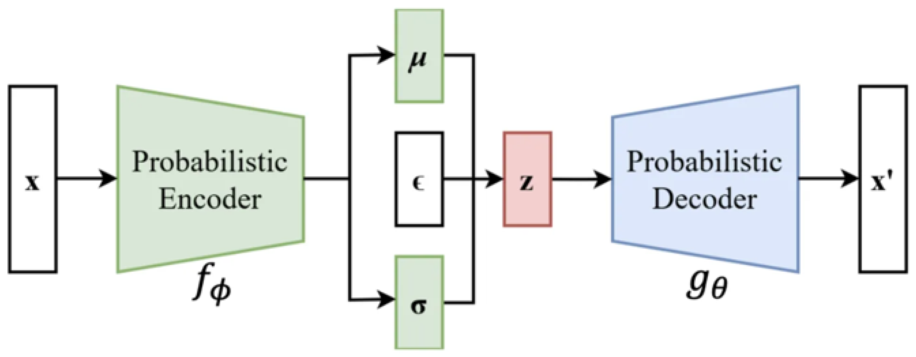
Appendix D. The Structure of VAE

Figure A1. The structure of VAE. The latent variable z N μ , σ 2 . .
Mathematics 12 00696 g0a1
Loss function:
F θ , ϕ ; x , z = E q ϕ z | x l o g p θ x | z D K L q ϕ z | x | | p z
where, x and z denote the observational data and latent vector, respectively. q ϕ denotes the distribution that the encoder learned from the data. D K L p 1 | | p 2 indicates the Kullback–Leibler divergence between p 1 and p 2 .

Appendix E. Model Settings

Below, we introduce the parameter settings of each model utilized in the comparison of the different datasets.

Appendix E.1. Linear Simulated Data

In this experiment, all models have a single-layer linear structure, and the output of the linear layer is mapped to the [0, 1] interval through a sigmoid function. We set the maximum number of iterations to 100,000. Training is terminated prematurely when the mean squared error (MSE) between the mean of the regression coefficients obtained in the last 100 iterations and the latest regression coefficients is less than 0.001. The learning rate is set to 0.1 in the fourth example, whereas in the other examples, the learning rate is set to 0.01.
IRM: For IRM, we set the penalty term coefficient λ to 2.
V-REx: For V-REx, we set the penalty term coefficient λ to 100.
RVP: For RVP, we set the penalty term coefficient λ to 10.
CoCo: For CoCo, we set the penalty term coefficient λ to 1.
ICP: For ICP, we selected a significance level of α = 0.05 . For the invariant features identified after the test, we used a linear layer followed by a sigmoid function as the predictor to map them to categories.

Appendix E.2. GMM

ERM: The ERM method employs a three-layer MLP (Multi-Layer Perceptron), with each hidden layer having a dimensionality of 10. The MLP uses the sigmoid function as its activation function. We set the maximum iterations to 2000. The learning rate is set to 0.01.
IRM: IRM employs an MLP with the same structure as ERM. The regularization term coefficient λ is set to 10. We set the maximum iterations to 2000. The learning rate is set to 0.01.
V-REx: V-REx employs an MLP with the same structure as ERM. The regularization term coefficient λ is set to 100. We set the maximum iterations to 2000. The learning rate is set to 0.01.
RVP: RVP employs an MLP with the same structure as ERM. The regularization term coefficient λ is set to 10. We set the maximum iterations to 2000. The learning rate is set to 0.01.
CoCo: CoCo employs an MLP with the same structure as ERM. The regularization term coefficient λ is set to 30. We set the maximum iterations to 2000. The learning rate is set to 0.01.
ICP: For ICP, we select a significance level of α = 0.05 in hypothesis testing.

Appendix E.3. Colored MNIST

The size of the images generated in this experiment is 2 × 14 × 14 .
ERM: The ERM method employs a three-layer MLP (Multi-Layer Perceptron), with each hidden layer having a dimensionality of 390. The MLP uses the ReLU function as its activation function. We set the maximum iterations to 3000. The learning rate is set to 0.0001.
IRM: IRM employs an MLP with the same structure as ERM. The regularization term coefficient λ is set to 900. We set the maximum iterations to 3000. The learning rate is set to 0.0001.
V-REx: V-REx employs an MLP with the same structure as ERM. The regularization term coefficient λ is set to 500. We set the maximum iterations to 3000. The learning rate is set to 0.0001.
RVP: RVP employs an MLP with the same structure as ERM. The regularization term coefficient λ is set to 50. We set the maximum iterations to 3000. The learning rate is set to 0.0001.
CoCo: CoCo employs an MLP with the same structure as ERM. The regularization term coefficient λ is set to 500. We set the maximum iterations to 3000. The learning rate is set to 0.0001.
ICP: For ICP, we select a significance level of α = 0.05 in hypothesis testing.

Appendix E.4. NICO

The size of the images used in this experiment is 3 × 224 × 224 .
ERM: ERM utilizes a combination of ResNet18 and two fully connected layers. The hidden layer of the fully connected layers has a dimensionality of 10, and the activation function used is the sigmoid function. We set the maximum iterations to 2000. The batch size during training is set to 100. The learning rate is set to 0.003.
IRM: IRM employs the same network structure as ERM, and the regularization term parameter is set to 100. The learning rate is set to 0.003.
V-REx: V-REx employs the same network structure as ERM, and the regularization term parameter is set to 50. The learning rate is set to 0.003.
RVP: RVP employs the same network structure as ERM, and the regularization term parameter is set to 5. The learning rate is set to 0.003.
CoCo: CoCo employs the same network structure as ERM, and the regularization term parameter is set to 500. The learning rate is set to 0.003.
ICP: For ICP, we select a significance level of α = 0.05 in hypothesis testing.

Appendix F. Generating Linear Simulated Data

Table A1. The formula for generating the data in Section 4.1. The environments are indexed by e, and γ e 0.5 , 1.0 , 5.0 .
Case 1Case 2Case 3
x 1 e N ( 0 , 1 ) x 2 e N ( 0 , ( γ e ) 2 ) x 2 e N ( 1 , ( γ e 2 ) 2 )
x 2 e N ( 0.5 , 1 ) x 1 e x 2 e + U ( 1 , 1 ) x 1 e x 2 e + U ( 0 , 1 )
y e δ 3 x 1 e + 2 x 2 e + N ( 0 , 1 ) > 1 x 4 e x 1 e + N ( 0 , ( 1 2 ) 2 ) x 3 e x 1 e + x 2 e + N ( 0 , ( 1 2 ) 2 )
z e γ e y e + N ( 0 , γ e ) y e δ 2 x 1 e + 1.5 x 4 e + N ( 0 , 1 ) > 0 y e δ x 2 e + 2 x 3 e + N ( 0 , 1 ) > 6
x 3 e γ e y e + N ( 0 , 1 ) x 4 e γ e y e + N ( 0 , 1 )
where δ f ( x ) > a takes a value of 1 when f ( x ) > a , and 0 otherwise.

Appendix G. Experimental Results

Figure A2. Input image and reconstructed image of β -VAE for Colored MNIST, where the image on the left is the input image and the image on the right is the reconstructed image.
Mathematics 12 00696 g0a2
Figure A3. Input images and reconstructed images of β -VAE for NICO, where the image on the left is the input image and the image on the right is the reconstructed image.
Mathematics 12 00696 g0a3

References

  1. Arjovsky, M.; Bottou, L.; Gulrajani, I.; Lopez-Paz, D. Invariant risk minimization. arXiv 2019, arXiv:1907.02893. [Google Scholar]
  2. Liu, J.; Hu, Z.; Cui, P.; Li, B.; Shen, Z. Heterogeneous Risk Minimization. In Proceedings of the 38th International Conference on Machine Learning, Virtual, 18–24 July 2021; Volume 139, pp. 6804–6814. [Google Scholar]
  3. Beery, S.; Horn, G.V.; Perona, P. Recognition in terra incognita. In Proceedings of the European Conference on Computer Vision (ECCV), Munich, Germany, 8–14 September 2018; Volume 16, pp. 472–489. [Google Scholar]
  4. Yin, M.; Wang, Y.; Blei, D.M. Optimization-based Causal Estimation from Heterogenous Environments. arXiv 2021, arXiv:2109.11990. [Google Scholar]
  5. Besserve, M.; Mehrjou, A.; Sun, R.; Schölkopf, B. Counterfactuals uncover the modular structure of deep generative models. In Proceedings of the Eighth International Conference on Learning Representations (ICLR 2020), Addis Ababa, Ethiopia, 26–30 April 2020. [Google Scholar]
  6. Pearl, J.; Glymour, M.; Jewell, N.P. Causal Inference in Statistics: A Primer; Wiley: Hoboken, NJ, USA, 2016. [Google Scholar]
  7. Peters, J.; Janzing, D.; Schölkopf, B. Elements of Causal Inference: Foundations and Learning Algorithms; MIT Press: Cambridge, MA, USA, 2017. [Google Scholar]
  8. Hendrycks, D.; Dietterich, T. Benchmarking Neural Network Robustness to Common Corruptions and Perturbations. arXiv 2019, arXiv:1903.12261. [Google Scholar]
  9. Shmueli, G. To Explain or to Predict? arXiv 2011, arXiv:1101.0891. [Google Scholar]
  10. Wang, R.; Yi, M.; Chen, Z.; Zhu, S. Out-of-distribution Generalization with Causal Invariant Transformations. In Proceedings of the IEEE/CVF Conference on Computer Vision and Pattern Recognition, New Orleans, LA, USA, 18–24 June 2022; pp. 375–385. [Google Scholar]
  11. Recht, B.; Roelofs, R.; Schmidt, L.; Shankar, V. Do ImageNet classifiers generalize to ImageNet? In Proceedings of the 36th International Conference on Machine Learning, ICML, Long Beach, CA, USA, 9–15 June 2019; pp. 9413–9424. [Google Scholar]
  12. Yi, M.; Wang, R.; Sun, J.; Li, Z.; Ma, Z.-M. Improved OOD Generalization via Conditional Invariant Regularizer. arXiv 2022, arXiv:2207.06687. [Google Scholar]
  13. Schneider, S.; Rusak, E.; Eck, L.; Bringmann, O.; Brendel, W.; Bethge, M. Improving robustness against common corruptions by covariate shift adaptation. In Advances in Neural Information Processing Systems 33; NeurIPS: La Jolla, CA, USA, 2020. [Google Scholar]
  14. Tu, L.; Lalwani, G.; Gella, S.; He, H. An empirical study on robustness to spurious correlations using pre-trained language models. Trans. Assoc. Comput. Linguist. 2020, 8, 621–633. [Google Scholar] [CrossRef]
  15. Muandet, K.; Balduzzi, D.; Schölkopf, B. Domain generalization via invariant feature representation. In Proceedings of the 30th International Conference on Machine Learning, ICML, Atlanta, GA, USA, 17–19 June 2013; PART 1. pp. 10–18. [Google Scholar]
  16. Su, H.; Wang, W. An Out-of-Distribution Generalization Framework Based on Variational Backdoor Adjustment. Mathematics 2024, 12, 85. [Google Scholar] [CrossRef]
  17. Scholkopf, B.; Locatello, F.; Bauer, S.; Ke, N.R.; Goyal, A.; Bengio, Y.; Kalchbrenner, N. Toward Causal Representation Learning. Proc. IEEE 2021, 109, 612–634. [Google Scholar] [CrossRef]
  18. Sinha, A.; Namkoong, H.; Duchi, J. Certifying some distributional robustness with principled adversarial training. In Proceedings of the 6th International Conference on Learning Representations, ICLR, Vancouver, BC, Canada, 30 April–3 May 2018. [Google Scholar]
  19. Sagawa, S.; Koh, P.W.; Hashimoto, T.B.; Liang, P. Distributionally Robust Neural Networks for Group Shifts. arXiv 2019, arXiv:1911.08731. [Google Scholar]
  20. Li, Y.; Tian, X.; Gong, M.; Liu, Y.; Liu, T.; Zhang, K.; Tao, D. Deep Domain Generalization via Conditional Invariant Adversarial Networks. In Proceedings of the 15th European Conference on Computer Vision, Munich, Germany, 8–14 September 2018. [Google Scholar]
  21. Chang, S.; Zhang, Y.; Yu, M.; Jaakkola, T. Invariant rationalization. In Proceedings of the 37th International Conference on Machine Learning, ICML, Virtual, 13–18 July 2020. [Google Scholar]
  22. Rojas-Carulla, M.; Schölkopf, B.; Turner, R.; Peters, J. Invariant models for causal transfer learning. J. Mach. Learn. Res. 2018, 19, 1309–1342. [Google Scholar]
  23. Shen, Z.; Cui, P.; Zhang, T.; Kunag, K. Stable Learning via Sample Reweighting. In Proceedings of the 34th AAAI Conference on Artificial Intelligence, New York, NY, USA, 7–12 February 2020; pp. 5692–5699. [Google Scholar]
  24. Schölkopf, B. Causality for Machine Learning. arXiv 2019, arXiv:1911.10500. [Google Scholar]
  25. Kuang, K.; Cui, P.; Athey, S.; Xiong, R.; Li, B. Stable prediction across unknown environments. In Proceedings of the ACM SIGKDD International Conference on Knowledge Discovery and Data Mining, London, UK, 19–23 August 2018; pp. 1617–1626. [Google Scholar]
  26. Peters, J.; Bühlmann, P.; Meinshausen, N. Causal inference by using invariant prediction: Identification and confidence intervals. J. R. Stat. Soc. Ser. Stat. Methodol. 2016, 78, 947–1012. [Google Scholar] [CrossRef]
  27. Cui, P.; Athey, S. Stable learning establishes some common ground between causal inference and machine learning. Nat. Mach. Intell. 2022, 4, 110–115. [Google Scholar] [CrossRef]
  28. Rosenfeld, E.; Ravikumar, P.; Risteski, A. The Risks of Invariant Risk Minimization. arXiv 2020, arXiv:2010.05761. [Google Scholar]
  29. Kamath, P.; Tangella, A.; Sutherland, D.J.; Srebro, N. Does Invariant Risk Minimization Capture Invariance? arXiv 2021, arXiv:2101.01134. [Google Scholar]
  30. Rubin, D.B. Causal Inference Using Potential Outcomes: Design, Modeling, Decisions. J. Am. Stat. Assoc. 2005, 469, 322–331. [Google Scholar] [CrossRef]
  31. Dawid, A.P. Causal Inference Without Counterfactuals. J. Am. Stat. Assoc. 2000, 95, 407–424. [Google Scholar] [CrossRef]
  32. Robins, J.M.; Hernón, M.Á.; Brumback, B. Marginal Structural Models and Causal Inference in Epidemiology. Epidemiology 2000, 11, 550–560. [Google Scholar] [CrossRef] [PubMed]
  33. Pearl, J. Causality: Models, Reasoning, and Inference; Cambridge University Press: Cambridge, UK, 2009. [Google Scholar]
  34. Greenl, S.; Pearl, J.; Robins, J.M. Causal Diagrams for Epidemiologic Research. Epidemiology 1999, 10, 37–48. [Google Scholar] [CrossRef]
  35. Spirtes, P. Single World Intervention Graphs (SWIGs): A Unification of the Counterfactual and Graphical Approaches to Causality; Working Paper Number 128; Center for Statistics and the Social Sciences University of Washington: Seattle, WA, USA, 2013. [Google Scholar]
  36. Richardson, T.; Robins, J.M. Causation, Prediction, and Search. MIT Press: Cambridge, MA, USA, 2000. [Google Scholar]
  37. Yao, L.; Chu, Z.; Li, S.; Li, Y.; Gao, J.; Zhang, A. A Survey on Causal Inference. Assoc. Comput. Mach. 2021, 15, 1–46. [Google Scholar] [CrossRef]
  38. Pearl, J. Causal inference in statistics: An overview. Stat. Surv. 2009, 3, 96–146. [Google Scholar] [CrossRef]
  39. Brand, J.E.; Zhou, X.; Xie, Y. Recent Developments in Causal Inference and Machine Learning. Annu. Rev. Sociol. 2023, 49, 81–110. [Google Scholar] [CrossRef]
  40. Hair, J.F., Jr.; Sarstedt, M. Data, measurement, and causal inferences in machine learning: Opportunities and challenges for marketing. J. Mark. Theory Pract. 2021, 29, 65–77. [Google Scholar] [CrossRef]
  41. Higgins, I.; Amos, D.; Pfau, D.; Racaniere, S.; Matthey, L.; Rezende, D.; Lerchner, A. Towards a Definition of Disentangled Representations. arXiv 2023, arXiv:1812.02230. [Google Scholar]
  42. Wang, X.; Chen, H.; Tang, S.; Wu, Z.; Zhu, W. Disentangled Representation Learning. arXiv 2023, arXiv:2211.11695. [Google Scholar]
  43. Kuang, K.; Xiong, R.; Cui, P.; Athey, S.; Li, B. Stable prediction with model misspecification and agnostic distribution shift. In Proceedings of the AAAI Conference on Artificial Intelligence, New York, NY, USA, 7–12 February 2020; Volume 34, pp. 4485–4492. [Google Scholar]
  44. George, C.; Roger, L.B. Statistical Inference; Duxbury Press: London, UK, 2001. [Google Scholar]
  45. Krueger, D.; Caballero, E.; Jacobsen, J.; Zhang, A.; Binas, J.; Zhang, D.; Priol, R.L.; Courville, A. Out-of-Distribution Generalization via Risk Extrapolation (REx). arXiv 2020, arXiv:2003.00688. [Google Scholar]
  46. Xie, C.; Chen, F.; Liu, Y.; Li, Z. Risk variance penalization: From distributional robustness to causality. arXiv 2020, arXiv:2006.07544. [Google Scholar]
  47. Higgins, I.; Matthey, L.; Pal, A.; Burgess, C.; Glorot, X.; Botvinick, M.; Mohamed, S.; Lerchner, A. beta-VAE: Learning Basic Visual Concepts with a Constrained Variational Framework. In Proceedings of the International Conference on Learning Representations, San Juan, Puerto Rico, 2–4 May 2016. [Google Scholar]
  48. Kingma, D.P.; Welling, M. Auto-Encoding Variational Bayes. In Proceedings of the International Conference on Learning Representations, ICLR, Banff, AB, Canada, 14–16 April 2014. [Google Scholar]
  49. He, Y.; Shen, Z.; Cui, P. Towards non-iid Image Classification: A Dataset and Baselines. In Proceedings of the Computer Vision and Pattern Recognition, CVPR, Long Beach, CA, USA, 15–20 June 2019. [Google Scholar]
  50. He, K.; Zhang, X.; Ren, S.; Sun, J. Deep Residual Learning for Image Recognition. In Proceedings of the 2016 IEEE Conference on Computer Vision and Pattern Recognition (CVPR), Las Vegas, NV, USA, 27–30 June 2016; pp. 770–778. [Google Scholar]
Figure 1. (a) The causal graph of modular variables. (b) The causal graph of non-modular variables. The black arrows represent the detgasssined causal relationships. The blue arrows represent the possible causal relationships, which are determined by the dataset.
Mathematics 12 00696 g001
Figure 2. The system architecture of the proposed algorithm. The black boxes represent the data, and the blue boxes represent operations on the data. The area inside the red dashed box represents the invariant causal inference process.
Mathematics 12 00696 g002
Figure 3. The causal graphs for the simulated data, where Y represents the target variable and the blue nodes represent the environmental variables. These structures are unknown during inference, and we infer environmental variables solely from the observed data. (a) The causal graph for Case 1. (b) The causal graph for Case 2. (c) The causal graph for Case 3.
Mathematics 12 00696 g003
Figure 4. Trace plots of testing accuracy for IFCI, ERM, V-REx, RVP, IRM, and CoCo. The horizontal coordinate represents the training epoch, and the vertical coordinate represents the accuracy of the models on the test set.
Mathematics 12 00696 g004
Figure 5. (a) The interpolation of latent features β -VAE extracted. Each row is a dimension of the latent vector. The color of the numbers corresponds to an environmental feature we added, which does not help predict the target variable, but there is a correlation between the color of the numbers and the target variable in the training set. (b) The results on the latent variables of IFCI.
Mathematics 12 00696 g005
Table 1. Predictive accuracy in training and testing environments for linear simulated data in Case 1, and the time it took for each model to converge during training. The bold numbers represent the optimal result.
AlgorithmTraining AccuracyTesting AccuracyTraining Time
ERM92.880.718.85 s
IRM90.283.917.72 s
V-REx90.086.817.70 s
RVP91.187.023.60 s
CoCo85.184.520.1 s
ICP93.692.319.69 s
IFCI93.692.318.03 s
Table 2. Predictive accuracy in training and testing environments for linear simulated data in Case 2, and the time it took for each model to converge during training. The bold numbers represent the optimal result.
AlgorithmTraining AccuracyTesting AccuracyTraining Time
ERM96.482.016.83 s
IRM94.483.617.36 s
V-REx93.077.234.50 s
RVP88.174.234.53 s
CoCo86.181.842.90 s
ICP---
IFCI94.291.516.96 s
Table 3. Predictive accuracy in training and testing environments for linear simulated data in Case 3, and the time it took for each model to converge during training. The bold numbers represent the optimal result.
AlgorithmTraining AccuracyTesting AccuracyTraining Time
ERM89.070.923.47 s
IRM89.680.916.33 s
V-REx86.874.634.47 s
RVP85.971.735.37 s
CoCo79.064.020.1 s
ICP89.070.919.69 s
IFCI91.288.315.03 s
Table 4. Predictive accuracy in training and testing environments for GMM, and the time it took for each model to converge during training. The bold numbers represent the optimal result.
AlgorithmTraining AccuracyTesting AccuracyTraining Time
ERM99.050.521.9 s
IRM93.188.032.24 s
V-REx92.785.917.70 s
RVP93.188.618.16 s
CoCo89.389.365.92 s
ICP---
IFCI91.891.716.96 s
Table 5. F-statistics of each dimension calculated in IFCI. In IFCI, the significance level α was selected as 0.05. C i represents the causal variable. E i represents the environmental variable. The bold numbers represent the recognized environmental variables.
C 1 C 2 C 3 C 4 C 5 E 1 E 2 E 3
1.190.270.230.120.803561.62 485.23589.32
Table 6. Classification accuracy in training and testing environments for Colored MNIST, and the time it took for each model to converge during training. The bold numbers represent the optimal result.
AlgorithmTraining AccuracyTesting AccuracyTraining Time
ERM99.147.430.30 s
IRM96.470.335.38 s
V-REx98.949.530.86 s
RVP98.556.933.92 s
CoCo93.588.792.24 s
ICP85.382.135.44 s
IFCI93.891.933.12 s
Table 7. Classification accuracy in training and testing environments for NICO, and the time it took for each model to converge during training. The bold numbers represent the optimal result.
AlgorithmTraining AccuracyTesting AccuracyTraining Time
ERM96.954.01648.6 s
IRM85.373.42351.2 s
V-REx95.669.12169.3 s
RVP92.173.72571.3 s
CoCo81.979.54687.2 s
ICP75.172.61990.5 s
IFCI83.181.71953.0 s
Disclaimer/Publisher’s Note: The statements, opinions and data contained in all publications are solely those of the individual author(s) and contributor(s) and not of MDPI and/or the editor(s). MDPI and/or the editor(s) disclaim responsibility for any injury to people or property resulting from any ideas, methods, instructions or products referred to in the content.

