1. Introduction
Optimal stopping problems are formulated in terms of observing random variables and determining the stopping time(s) in order to maximise an objective function (which can be thought of as some reward). The discrete single-stopping problem involves observing a sequence of random variables
, and making the choice to stop on a particular observation
, where
, which is based only on the variables that have been previously observed. After stopping, the “player” receives some pay-off which is a function of the variables observed
. In [
1], we used the pay-off of
(i.e., the value of the variable stopped on). To extend this to the multiple optimal stopping problem we stop on
variables and, after stopping on variables
at times
, we then receive a gain which is a function of the variables observed. This problem is a subset of a general class of other optimal stopping problems that all aim to find a sequential procedure to maximise the expected reward (see Section 13.4 of [
2] for a more extensive discussion of this class of problem). The secretary problem is arguably the most well known (see [
3,
4]), and it has a wide range of variations (see [
5,
6]), but there is also a rich literature of other examples (see [
7]). By the ‘duration’ (sometimes referred to as ‘time’) of the stopping problem, we refer to how many observations the statistician observes before optimally stopping. It should be emphasised that knowing how long you would be waiting, on average, for potentially large sequences of observations is also useful to understand (see [
8]), which highlights the need for asymptotic analysis to address this question.
Less focus has been placed on understanding the asymptotic behaviour of the stopping duration, with most pre-existing results focusing on secretary-type, so called “no-information”, problems where the distribution of the observations is unknown. The asymptotic expectation and variance of the stopping time for the secretary problem were studied in [
9]. Similar asymptotic analyses for other variants of no-information problems can be found in [
10,
11,
12,
13], where the techniques/formulations used differ depending on the particular variation or structure of the problem.
There is substantially less literature describing the asymptotic behaviour for “full-information” problems, when the distribution of the variables is known a priori. A smaller subset addresses the multiple stopping problem, which we focus on in this study.
Gilbert and Mosteller [
11] studied the optimal stopping strategy for the full-information problem in which the objective is to maximise the probability of attaining the best observation, known as the full-information best-choice problem [
14]. The optimal rule was shown to be a threshold strategy wherein the player would stop on
if it was the best observed so far after all other observations and its value exceeded a threshold that depended on
m. The asymptotic behaviour of this rule was also derived.
In the full-information case, the pay-off can instead be in terms of the actual values of the variables stopped on. A special case of this is the uniform game (see Section 5a of [
11]), which is closely related to Cayley’s problem (see [
3,
15]). In [
11], the authors showed an asymptotic expression for the expected reward of a sequence of
n independent and identically distributed (iid) random variables having the standard uniform distribution (see also [
15]). In [
9], Mazalov and Peshkov found the asymptotic behaviour of the expected value and variance of the stopping time as
and
, respectively, when the variables are from the uniform distribution. However, the techniques applied were specific to the structure of the distribution, and thus, it is difficult to easily extend or generalise this to other distribution functions. In [
16,
17], using the extreme value theory, Kennedy and Kertz proved limit theorems for threshold-stopped random variables and derived the asymptotic distribution of the reward sequence of the optimal stopping (iid) random variables. The asymptotic pay-off for the multiple case is briefly analysed in (Section 5c of [
11]).
In [
1], we outlined a novel approach for a general asymptotic technique for calculating the asymptotic behaviour of the pay-off as well as
and
in the single-stopping case, where
is the single-stopping time, as
for general classes of probability distributions in the full-information problem where we wish to maximise the expected reward
. The techniques in our previous paper, which are extended in this study, employ the asymptotic analysis of difference and differential equations in order to establish and solve asymptotic differential equations for the quantities of interest. Differential equations were also used in [
18,
19]. In this study, we extend some of our results in [
1] to the multiple stopping case through some inductive arguments and verify these results with simulations. For simplicity, we only analyse continuous distributions and reserve the notation
, and
for the continuous probability density, cumulative distribution, and “survivor” function, respectively. We use the notation
∼
to establish the asymptotic relation that
.
2. Formulation of the Multiple Optimal Stopping Problem
As in the single-stopping problem, we still sequentially observe the sequence
of independent, identically distributed (iid) random variables from a known distribution, we must decide which
k of these variables to stop on. After
k,
stoppings at times
, where
, we receive the gain
The random variable
can be interpreted as the value of some asset, such as a house, at time
m. The problem of selling
k identical objects in a finite time (or horizon)
N with one offer per time period and no recall of previous offers is analogous to the multiple optimal stopping problem described. If we stop at
after observations (
,
,…,
), then we proceed to observe another sequence
(whose length depends on
) and must solve the new optimal stopping problem on this sequence. From [
20], we have the following theorem.
Theorem 1. Let be a sequence of independent random variables with known cumulative distribution functions (cdfs) . Let be the value, which is the optimal expected reward, of a game with l, stoppings and L, steps. If there exist , then the value v of the ‘game’ is , whereWe putthen, is the optimal stopping rule. If we define
, then we may notice that the stopping rules now take the form
so we may interpret
as the appropriate threshold value that needs to be satisfied for stopping for the
ith occasion at the
jth term in the sequence of
N observations. We can then define
, which can now be interpreted as the probability that in the above situation we do
not stop.
Example 1 (Multiple Stopping on the Uniform (0, 1) Distribution with
stops)
. Let be a sequence of independent, identically distributed random variables that follow the uniform distribution.
We derived the equations for
in the original paper (for details, see [
1]):
where
. For
we have that
which can then be used to numerically determine the values of the ‘game’.
For the example of
, we may produce the values for
and
for each value of
n from
to
, as displayed in
Table 1. For example, consider this sequence of simulated variables:
For the first stop, we would arrive on
, since
is the first variable to satisfy
and for the second, we arrive on
, as this is the first subsequent variable for which
. This particular example would have resulted in the reward
3. Computing Behaviour
We establish a similar recurrence result as we did for the single-stopping case. We note that this relation for
will now be a second-order relation. For a convenient evaluation of the expectation, we use the fact that for any continuous integrable random variable
X with cdf
, the expectation can be given by
Theorem 2. Let Y be an integrable random variable whose expectation exists, and which is drawn from a continuous probability distribution function (pdf) with survivor function . The value of a sequence with steps and k stops remaining is given by Proof. For ease of notation, we let
. Then, by definition, we have
where the last expectation, using (
3), is given by
Substituting this result, noting that the
terms cancel, we obtain the required result. □
We note that if
has bounded support in the positive direction such that
for
, it follows from above that
By the controlling factor method, we also have that
, which can be combined with the previous integral to establish the following:
This may be differentiated on both sides to obtain the asymptotic relation for the second derivative:
This expression can now be rearranged for
to give
Depending on the asymptotic nature of and their derivatives, this result can be used through direct substitution. In other scenarios, the derivative expressions may not yield useful expressions and the behaviour of can be analysed directly without this result. We will provide variations of this in the subsequent example calculations.
Example Calculations
We illustrate the application of these ideas to some common distributions, such as the uniform and exponential distributions. However, the nature of the differential equations that arise from the multiple stopping problem are much harder to solve—some of them have no solution.
Example 2. The uniform distribution is given by on , where .
For the differential equation for the large asymptotic behaviour, we have that
. Defining
and rearranging in the asymptotic relation for
we obtain
From [
1], we have the asymptotic relation
, which can be directly substituted into the above equation:
We can solve this formal differential equation to obtain
where
c arises as a constant of integration but may be dropped since it is part of a sub-dominant term. We now replace
v with
, substitute our asymptotic relation for
, and rearrange for
to obtain
We may notice, in general, that whenever
v satisfies the relation
where
is some positive constant, that we obtain the asymptotic relation
This can be used to generalise the asymptotic behaviour for
for the uniform distribution.
Theorem 3. Consider to be independent identically distributed uniform variables on , . The reward sequence follows the asymptotic relationwhere for and . Proof. We have shown this to be true for
and
. Now, assume that
Now define
, we have
which, from (
10) and (
11), has the asymptotic solution
To conclude the proof, we rearrange for
to obtain
□
We noted in [
1] that the behaviour of
was identical for the family of distributions with exponential tails. The next example will seek to unify such distributions that corresponded to
in the multiple stopping scenario.
Example 3. A continuous probability density function is given with a survival function that, for sufficiently large y, satisfiesfor positive Δ, and where β and γ are positive constants. Assume each of the terms in the sequence of reward values increases without bound. We obtain the ordinary differential equation
where
represents the upper incomplete gamma function, and
which is sub-dominant in the asymptotic differential equation. The solution to the differential equation is thus approximated by
This gives
We have, from [
1],
, and so the general case for
may be presented by mathematical induction.
Theorem 4. Let be random variables from a distribution that, for sufficiently large y, satisfiesfor positive Δ, and where β and γ are positive constants. Assume each of the terms in the sequence of reward values increases without bound. Then, the asymptotic behaviour of is given by Proof. From (
15) we have that the behaviour of
is related by
We have verified the claim for
in [
1]. We now assume that
as
and use this to prove the same for
. We write the asymptotic differential equation
and substitute for our assumed asymptotic for
to obtain
which is a separable differential equation with solution
as required. □
4. Calculating the Optimal Expectation
In this section, we continue the ideas from the single-stopping calculation to calculate the expectation for the multiple stopping rules. We proceed to find the asymptotic for the expected value , the first stopping time. We can then find the rest of the expectations in an inductive fashion under certain conditions. We now extend some of the previous notation to reflect the multiple reward sequences, as well as k stopping variables. Let denote the 1st, 2nd, …, kth stopping times, respectively, and let .
5. An Asymptotic Equation for
By recalling the notation from the beginning of this section, we obtain
through
We split the summation for
on a value
, where
:
where we apply the fact that
to obtain a bound for the first summation term:
For the second summation term, as
is large in the limit as
, we may use the asymptotic approximations for
obtained in the previous section.
For many distributions, this can be simplified through using the large-
n asymptotic for
and its derivatives, or obtaining an asymptotic expression for
through other means. In the case where
, we have from [
1] that
Example 4. Uniform Distribution for k stops.
For simplicity, we first consider the double stopping problem (
). From Example 2, we have that
This obtains
, and thus,
We then have that
For the general result with
stops for the uniform distribution, we apply the asymptotic behaviour of
to obtain
For
, conveniently
, this retrieves
. For
, we have that
, and so, this retrieves
, consistent with our previous results.
Example 5 (Distributions with an Exponential Tail (
k stops))
. We once again consider a probability distribution is given with a survival function that, for sufficiently large y, satisfieswhere the additional conditions are described in Example 3. We found that the sequences
satisfy the asymptotic relation
and so
From this we obtain asymptotic relations for the derivatives:
Hence, we obtain
Provided that
is asymptotically of this form, we may make use of linearity of expectation to obtain convenient conditional formulae that are not as complicated as those encountered in the previous section.
6. An Inductive Approach for
Due to the independence of observations, it starts to make physical sense to view the expectation of the th stopping time as a function of only the previous stopping time. We, thus, investigate the properties of the th stopping time when conditioned on the jth. We would expect then to only need to add the additional expected number of observations to stop one more time out of a ‘reduced’ optimal stopping problem. We now introduce the notation to allow for more flexible interactions between stopping times.
Definition 1. Let denote the jth stopping time (out of k) in the optimal stopping problem with N observations.
Here, denotes the used in the previous section. corresponds to the in the single-stopping problem.
Theorem 5. Let be independent and identically distributed random variables where the expectations of the optimal stopping times exist. Suppose further that the first stopping time out of k stops has asymptotic expectation for some constant . Then, the following relation holds:where is some other positive constant. Proof. We first show that the conditional expectation,
, is given by
where the last equality follows directly from the definition of
in the previous section. By the assumption of the form of the expectation, we thus have that
and so through linearity properties of expectation, as well as the law of total expectation, we finally obtain
□
This has a reasonable physical interpretation as we would expect that the expectation of the th stopping time will be the expectation of the jth stopping time as well as the additional time it would take to stop one more time in the revised stopping problem to stop at the next observation. This revised stopping problem has a reduced number of observations on average, as well as stops remaining since we have already stopped j times out of the original k times. A consequence of this theorem is that the asymptotic expectations may all be considered linear.
7. Asymptotic Equations for
We now demonstrate how the ideas discussed in the previous section can be applied to obtain all of the multiple stopping times for some classes of distribution. Simulations were also conducted to support the asymptotic calculations in this study.
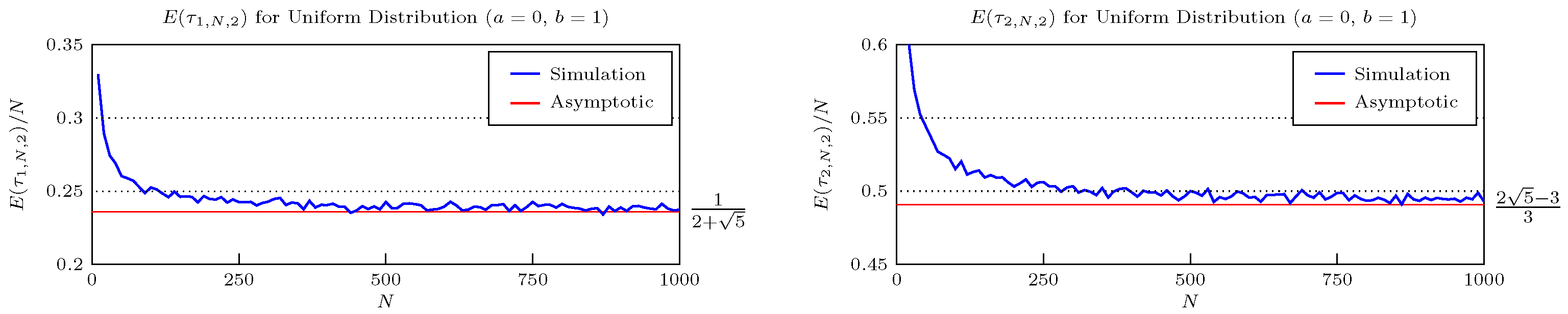
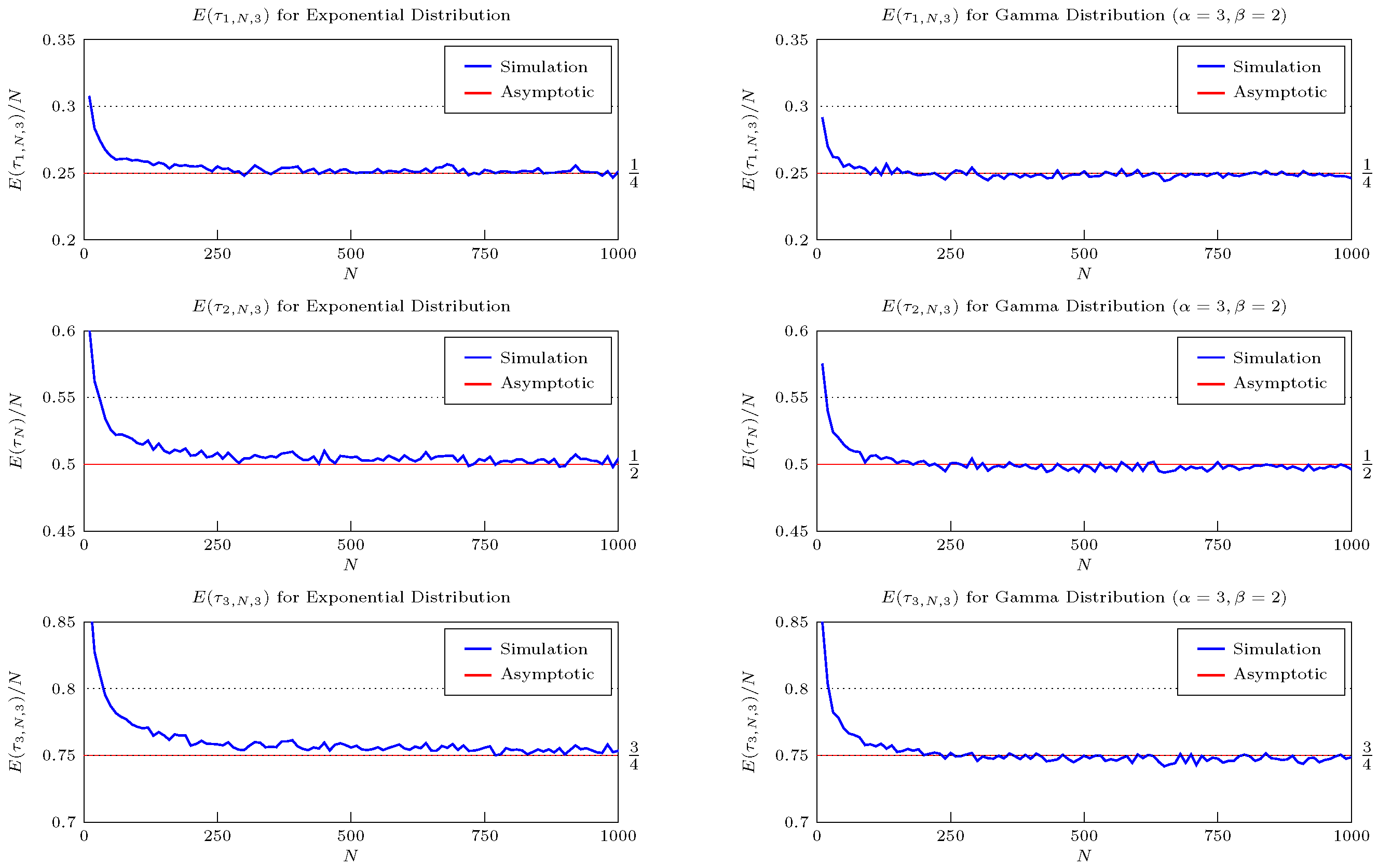
Figure 1 compares the large-
N asymptotic predictions for the expected duration for the standard uniform distribution under the optimal double stopping rule and
Figure 2 shows a similar comparison under a triple stopping rule for the exponential and the gamma distribution. In this section, we will now adopt the previous notation for the
jth stopping time out of
k, for
N observations as
.
These results were verified by simulation (see
Figure 1) which show the realised expectation converging to the asymptotic prediction. This procedure can be extended to calculate further results for more stopping times permitted. Simulation results (see
Figure 2) for the exponential and gamma distribution further support these asymptotic calculations.
Example 6 (Double Stopping on the Uniform Distribution)
. For the uniform distribution, we obtain an asymptotic expression for the first stopping time out of k stops. It is given bywhere is defined through the recursive scheme We can then apply Equation (
21), for the example of the double stopping case, recursively to obtain
and
.
Example 7 (Multiple Stopping on Distributions with Exponential Tails)
. We saw that the expressions can get somewhat out of hand for the uniform distribution. However, the structure can sometimes behave nicely to lead to a closed form result that need not be recursively evaluated. This is true for the class of distributions outlined in Example 3. We prove the following theorem for the general asymptotic expectation:
Theorem 6. Let be independent and identically distributed random variables. Define to be the jth stopping time out of k stops for the sequence of N observations. If , then we have that Proof. We see that the base case is in agreement; we now proceed with the inductive argument that
□


