A Convolutional Neural Network-Based Auto-Segmentation Pipeline for Breast Cancer Imaging

Abstract

Medical imaging is crucial for the detection and diagnosis of breast cancer. Artificial intelligence and computer vision have rapidly become popular in medical image analyses thanks to technological advancements. To improve the effectiveness and efficiency of medical diagnosis and treatment, significant efforts have been made in the literature on medical image processing, segmentation, volumetric analysis, and prediction. This paper is interested in the development of a prediction pipeline for breast cancer studies based on 3D computed tomography (CT) scans. Several algorithms were designed and integrated to classify the suitability of the CT slices. The selected slices from patients were then further processed in the pipeline. This was followed by data generalization and volume segmentation to reduce the computation complexity. The selected input data were fed into a 3D U-Net architecture in the pipeline for analysis and volumetric predictions of cancer tumors. Three types of U-Net models were designed and compared. The experimental results show that Model 1 of U-Net obtained the highest accuracy at 91.44% with the highest memory usage; Model 2 had the lowest memory usage with the lowest accuracy at 85.18%; and Model 3 achieved a balanced performance in accuracy and memory usage, which is a more suitable configuration for the developed pipeline.

1. Introduction

In recent years, a convergence of multiple factors has led to an exacerbating global shortage of radiologists. Examples of such factors include the rising demand for medical imaging, the coronavirus disease pandemic, and global aging. Over the past decade, artificial intelligence (AI) has been rapidly adopted in different industrial sectors. Similar to the ways humans carry out complex problem solving and decision making, AI is now able to perform learning from relevant datasets for various applications [1,2].

In the healthcare industry, radiology was one of the first medical disciplines to utilize computer vision (CV) for its medical applications [3]. As a subfield of AI, CV has a rich history spanning decades of research work to enable computers to meaningfully interpret visual stimuli. The development of CV has recently been accelerated due to three main factors: (1) the massive improvement in computer processing capability; (2) the rise of big data with the amassment and storage of a large amount of data; and (3) the increased contributions from machine learning algorithm research. CV systems can be used to analyze medical images such as CT scans, X-rays, and magnetic resonance images (MRIs). Convolutional neural networks (CNNs) are one of the mainstream methods in the field of medical imaging segmentation due to their performance [4,5,6,7]. Breast cancer is a type of common cancer in females in the world. An MRI segmentation model with a CNN was developed for the volumetric measurement of breast cancer [4]. Pre-trained CNN models were used for feature extraction in the task of detecting breast cancer in mammography images [5]. A dual-modal CNN was introduced to analyze both ultrasound (US) images and shear-wave elastography for the prediction of breast cancer [8]. A Regional Convolutional Neural Network (R-CNN) was utilized for MRI analysis to detect breast tumors [9]. Another R-CNN-based framework was reported for the MRI analysis and detection of breast cancer pathological lesions [10]. A deep learning-based tumoral radiomics model for CT images was introduced to predict the pathological complete response [11]. A CNN model was used for the delineation of the clinical target volumes (CTVs) in CT images of breast cancers in radiotherapy [6]. It was observed that the performance of CNN-based segmentation of CTVs in CT images of breast cancer was better than that of the manual process [12]. A CNN was depicted for the classification and detection of tumor cancers in CT scans [13]. These systems may be able to detect cancerous tumors with certain precision for small patches of anomalous tumor segments. Radiologists can fail in their process of cancer identification [14,15] due to the levels of their expert knowledge and experience. CV systems are complementary tools that can be used to support the work of radiologists and reduce diagnostic times.

Carrying out volumetric predictions of breast cancers in 3D CT scans is a challenging task depending on the experience of the radiologist. It would be beneficial to have an automatic framework using AI models for accurate volumetric predictions of tumors.

In this research, a CNN-based prediction pipeline is proposed for the volumetric prediction of breast cancers in 3D CT scans. The prediction pipeline consists of a suitable and accurate 3D CNN model, which is trained on CT scan datasets. As a type of CNN model, the U-Net architecture is capable of obtaining good precision with little training data. The CT scans of a total of 347 patients were provided by the National Cancer Centre, Singapore (NCCS) for the pipeline’s development. It is necessary to note that not all data are suitable for model training. The proposed pipeline is able to perform data pre-processing and manipulation to automatically select the proper data. The architecture of the U-Net in the pipeline was crafted and configured. Experiments were conducted to evaluate the performance of the pipeline outputs.

The main contributions of this paper are as follows:

(1)

A prediction pipeline is proposed, utilizing a 3D U-Net architecture for image segmentations in 3D CT scan images. The developed pipeline consists of a series of algorithms for data pre-processing to generalize and normalize the CT scan data. A 3D U-Net architecture is customized to cater to the requirements of accurate segmentations and volumetric predictions of breast tumors. The designed pipeline can become a complementary supporting tool for radiologists to increase the productivity and efficiency of their jobs.

(2)

For the U-Net architecture in the developed pipeline, a hybrid Tversky–cross-entropy loss function is utilized, which combines the advantages of the binary cross-entropy (BCE) loss function and the Tversky focal loss. A Nesterov-accelerated adaptive moment estimation (Nadam) optimization algorithm is leveraged to achieve better optimization performance.

(3)

Three types of 3D U-net architecture models are designed and compared in this research. Their performance is evaluated based on the Dice coefficient metric [16].

The organization of the remaining parts of the paper is as follows. Section 2 introduces the relevant background knowledge. Section 3 presents our methodology and design. Section 4 discusses the experiment results. Section 5 concludes the research.

2. Background Knowledge

2.1. CNN and U-Net

CNN is a variant of deep learning artificial neural networks. It is good for pattern recognition and image analysis in CV. The architecture of CNN consists of convolution layers [17,18]. These layers help identify patterns in images through a set of filters to detect edges and lines from previous layers. It then identifies the whole shapes and objects at later layers. Apart from the convolution layer, the activation layers, pooling layers, and fully connected layers are also important for a CNN [19]. Over the years, various types of CNN architectures were reported to cater to different applications. Some of the commonly seen architectures are shown in

Table 1. Various CNN architectures in the literature.

Type	Properties
LeNet [20,21]	First CNN architecture reported in 1998. Used for handwritten digit recognition. Suffered from vanishing gradient problem.
AlexNet [22,23]	Deeper, bigger, and stacked convolutional layers compared to LeNet. Used on large-scale image datasets. Rectified Linear Unit is used as an activation function, with batch size of 128.
ZFNet [24,25]	Reduced filter size in the first convolutional layer. Fewer parameters than AlexNet but with better performance. Hyperparameters are different from AlexNet.
GoogLeNet [25,26]	CNN proposed by Google. Deeper architecture due to 1 × 1 convolution and global average pooling. Computationally expensive.
VGGNet [25,27]	16-layer CNN for VGG16 architecture, with 13 convolutional layers and 3 fully connected layers. Can take large input image of 224 × 224-pixel size.
ResNet [25,28]	Utilized skip connections technique to address the vanishing gradient problem. Can be used for tasks of natural language processing. Computationally efficient to match the computation power of Graphics Processing Units (GPUs).
MobileNets [29]	Used depth-wise convolutions to apply a single filter into each channel. Introduced two hyperparameters: width multiplier and resolution multiplier. Can work on mobile devices for mobile and embedded vision applications, such as object detection, face recognition, etc.
U-Net [30,31]	Used for semantic segmentation to address the challenge of limited medical data with annotations. Consisted of a contracting path and an expansive path (i.e., encoder and decoder). Designed to work with fewer training images but yield favorable precision and computational efficiency.

.

U-Net is a type of deep CNN architecture suitable for biomedical image analysis [7,30]. U-Net-based architectures are one of the widely used structures in the field of medical image segmentation, such as breast tumor image segmentation, as it can work with small training data yet produce accurate results of image segmentation [32,33]. The U-Net architecture derives its U-shape due to the sequentially arranged encoder and decoder modules [30,31,34]. The encoder consists of convolutional layers, batch normalization (BN) function, activation layers, and max pooling layers to realize the unique features in a given image. The decoder combines the encoded spatial and feature information through up-convolutions and concatenations to produce a high-resolution image. This image provides the localized information needed for semantic segmentation.

The configurations of the original U-Net architecture can be fine-tuned with the different arrangements of the layers in the architecture. While designing a U-Net from scratch is possible, minor improvements to the existing architecture could be a quicker alternative, as observed in similar works [32].

2.2. Image Segmentation

Image segmentation is an image processing technique used to identify specific objects in an image [11,35,36]. Images can be divided into various partitions known as segments. Each segment is analyzed and assigned with some values. There are three common categories for segmentation tasks: binary segmentation, active contour segmentation, and semantic segmentation. The binary segmentation utilizes the threshold method, where a histogram of unique pixel values is extracted. This is followed by choosing a suitable threshold value, to derive the resultant output as a binary segmented image [33]. For the active contour segmentation, a boundary is first initialized around the object of interest, and it will automatically move towards the object. It is marked via the difference in pixel values, using a check iteration algorithm. The final boundary is the segmented image [37].

When dealing with more complicated images, semantic segmentation can be used, which involves labelling each pixel of an image corresponding to a specific class [38]. For example, if there are three unique classes namely Human, Bicycle, and Background, every object of the same class is labelled with the same pixel values. There is no distinction between different humans in the same class.

3. Methodology

3.1. Proposed Structure of the Volumetric Prediction Pipeline

There are three axes, i.e., x, y, and z, for the 3D CT scans for each patient. The breast cancer CT scan images contain a stack of images, depending on the spatial locations. The number of slices in the coronal plane and sagittal plane for each patient is the same, while the number of slices of each patient is unequal in the axial plane (i.e., z-axis). For example, scans of every patient have dimensions of 512 × 512 × n, where n varies for every patient, as shown in Figure 1. This is due to the nature of CT scanning machines. However, this can affect the U-Net model training, as typically it requires training data with equal spatial dimensions. It is, thus, necessary to derive suitable data by performing some data pre-processing on the CT slices, before feeding them into the proposed prediction pipeline.

The structure of the volumetric prediction pipeline is shown in Figure 2. It consists of a series of algorithms to filter CT scan slices step by step, which is from the input data to the 2D and 3D prediction visualization outputs.

(1)

An algorithm is developed to extract the number of slices in the axial plane for each patient.

(2)

The model training in the pipeline requires tumor labels, i.e., masks to be assigned to each slice. The slices without masks are filtered out from the training. Another algorithm is designed to identify which slices of each patient have associated masks. The indexes of such slices with masks are sorted out for each patient.

(3)

To ensure consistent training and better prediction performance, the pipeline requires the same ranges of slice spatial locations in the z-axis for all patients. The patients are classified into three categories based on the threshold value of the slice indexes at the z-axis. Only the slices from the patient category whose slice indexes are all smaller than or equal to the threshold value are selected for further processing.

(4)

The selected patient category is further classified into two groups based on the CT scan thickness.

(5)

The values of CT scan image matrices are normalized into the range of 0 to 1.

(6)

The 3D volumes with large dimensions require a large amount of GPU resources in the model training. They are divided by an algorithm into a set of cuboids with smaller dimensions to reduce computation complexity.

(7)

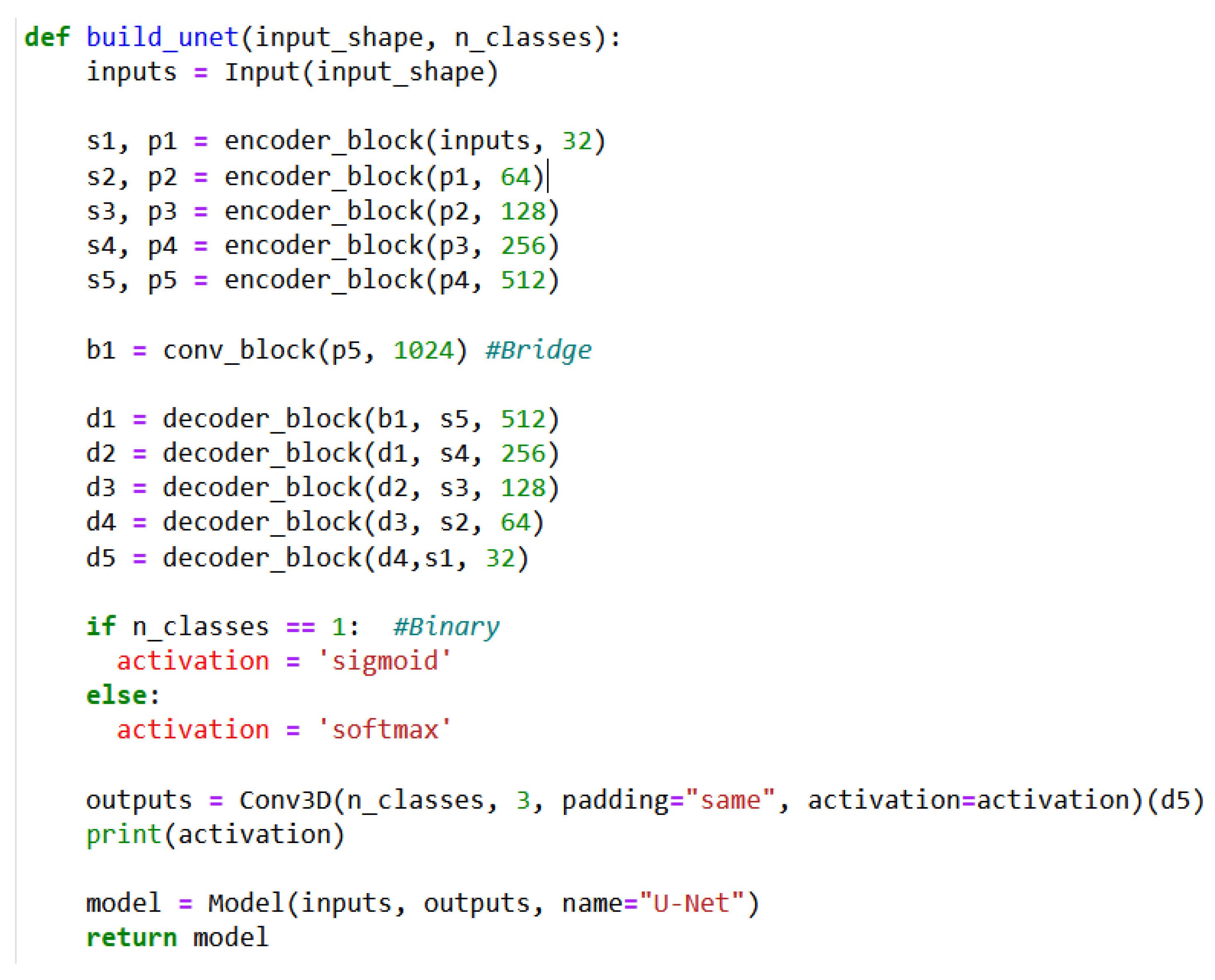
A 3D U-Net architecture is customized and trained for the image segmentation tasks with a hybrid loss function and a hybrid optimizer.

(8)

The results of 2D and 3D prediction results are visualized.

3.2. Detailed Data Pre-Processing Steps

The Python programming language is utilized in this research. Python libraries such as Tensorflow and Keras are used to assist in building of the U-Net architecture. The computer used in the experiment includes an Intel Xeon W-2265 12 core processor, 264 GB RAM, and 4 Nvidia Quadro RTX 5000 each with 16 GB GDDR6 memory for model training.

The CT scans obtained from 347 patients are provided by NCCS in the format of nearly raw raster data (.nrrd). The data are split into training, validation, and testing sets in the ratio of 60:20:20, corresponding to 210, 60, and 77 patients, respectively. The “pynrrd” Python library and “matplotlib” library are utilized in processing the CT scans and visualizing the data. The CT scans for each patient form a 3D volume. The CT scans are typically anisotropic. In order to gain a better understanding of the number of slices per patient in the axial plane, an algorithm is designed to extract the number of slices in the axial plane (Figure 3). It inspects all the data and counts iteratively the slices in the z-axis under the same patient. The final count of the slices in the z-axis per patient is the number of slices in the axial plane. The output of the extracted number of slices per patient is shown in Figure 4.

The training, validation, and testing of the U-Net model require the CT scan images with their respective masks. But the dataset of the CT scan images from 347 patients has masks for some of the slices. Therefore, an algorithm is developed to iteratively record the slice indexes consisting of corresponding masks for each patient, with the flow chart shown in Figure 5. The slice indexes are appended to the mask list under each patient.

Some sample outputs derived by the algorithm are shown in Figure 6. For example, there are a total of 122 slices for patient 1, but only six slices contain the masks with the slice indexes 85–90. We also note that a single patient out of 347 patients has no slices with masks. As such, only the slices of 346 patients are used in the proposed pipeline.

It is observed from the output of the slices with masks under each patient that there are different numbers of slices with masks in the axial plane. To resolve this issue of the unequal number of slices with masks in the axial plane, an algorithm is developed to classify the patients based on a threshold value of the slice indexes in the z-axis. The threshold value in the z-axis is set to 96, and a fixed spatial size of 512 × 512 × 96 is utilized in the proposed pipeline. This is in order to have the same ranges of spatial locations at the z-axis for CT scan slices, with data consistency for all patients. This means that the slices with masks in the range of the 1st–96th indexes for the patients will be used in the model training, validation, and testing.

As such, the 346 patients will be classified into three categories using another algorithm, shown in Figure 7, according to the indexes of slices with masks:

(1)

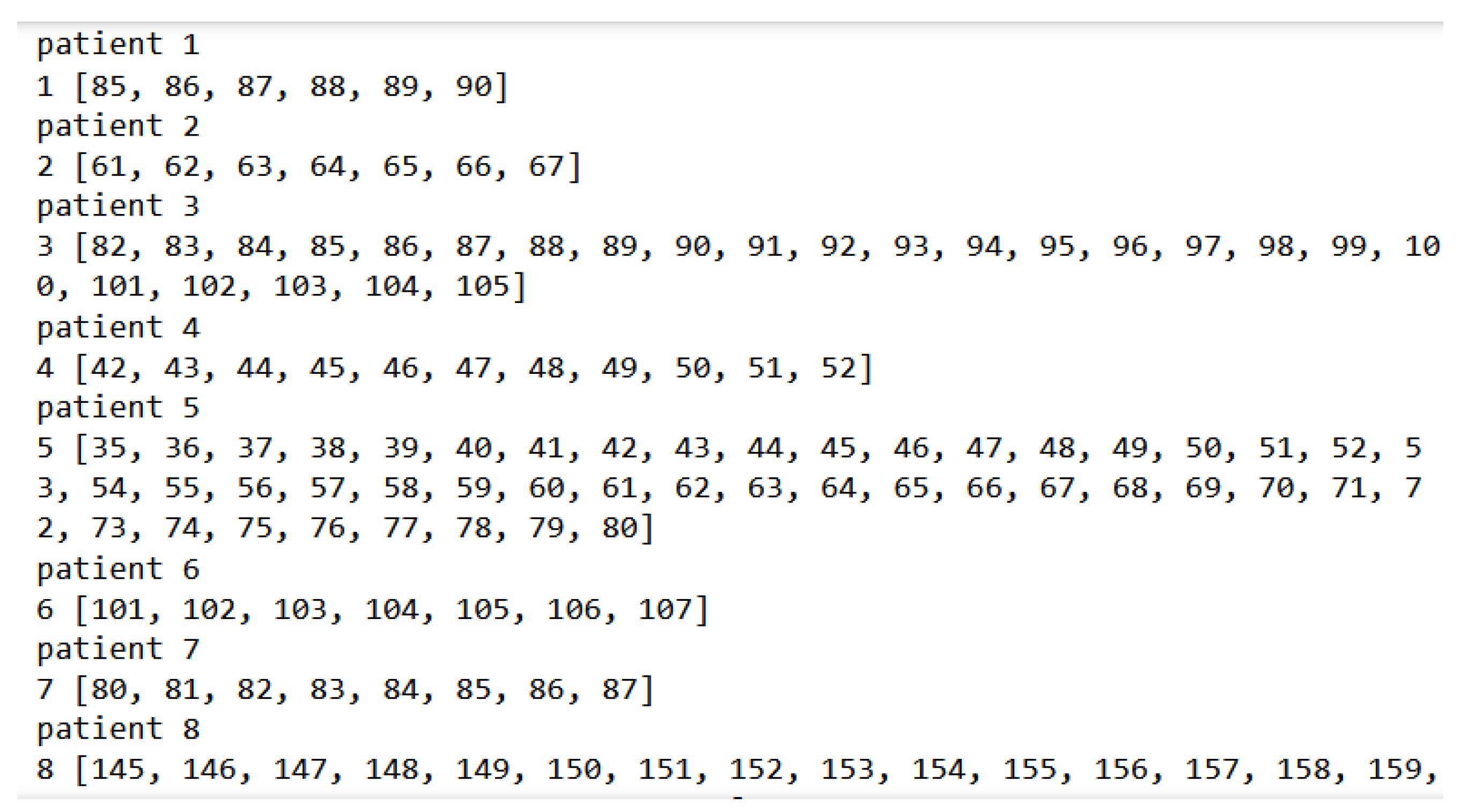
The List with all indexes ≤ 96: All indexes of the slices with masks are lesser than or equal to 96. As shown in Figure 6, most patients, e.g., patients 1, 2, 4, 5, and 7, satisfy this condition.

(2)

The List with all indexes > 96: All indexes of the slices with 96 masks or more. As shown in Figure 6, patient 6 and patient 8 are some examples.

(3)

The overlap list: Indexes of the slices with masks across all 96 indexes, where some indexes are lesser than or equal to 96, and the others are more than 96. As shown in Figure 6, patient 3 is the only patient that satisfies this condition.

With this algorithm, the CT scans of the 346 patients are classified into three categories, as shown in

Table 2. Obtained distributions of three categories of patients.

Mask Slice Presence	No. of Patients	Train Patients	Valid Patients	Test Patients
Index ≤ 96	191	109	43	39
Index > 96	91	58	9	24
The overlap	64	42	8	14
Total	346	210	60	77

. In the pipeline, only the patients whose indexes of the slices with masks are all ≤96 are utilized. Thus, only 191 patients are available for the model training, validation, and testing.

Besides the indexes of the slices with masks for each patient, another important parameter is the thickness of CT scans. In general, there are two thicknesses, namely 3 mm and 5 mm. The distributions of the thickness of the 191 patient scans are shown in

Table 3. Distribution of patient scan thickness.

CT Scan Thickness	Train Patients	Valid Patients	Test Patients	Total Patients
3 mm	74	26	27	127
5 mm	35	17	12	64
Total	109	43	39	191

, where the CT scans of 127 patients have a scan thickness of 3 mm. Since there are more patients with 3 mm scan thickness, they are used for the initial model training. The patient indexes of these 127 patients are shown in

Table 4. The 127 patients with 3 mm CT scan thickness.

Patient Category	Patient Index
Patients for Training	4, 5, 9, 10, 15, 16, 18, 19, 20, 21, 22, 23, 28, 29, 33, 34, 35, 37, 44, 51, 52, 58, 64, 68, 69, 72, 73, 76, 77, 79, 82, 83, 90, 91, 92, 93, 94, 95, 97, 103, 104, 116, 123, 126, 129, 131, 134, 136, 139, 142, 149, 151, 155, 157, 159, 162, 163, 164, 169, 170, 171, 179, 180, 186, 188, 191, 192, 198, 200, 201, 206, 207, 208, 209
Patients for Valid	213, 214, 215, 217, 219, 220, 221, 224, 226, 227, 228, 231, 237, 238, 240, 243, 248, 249, 250, 254, 255, 256, 257, 264, 266, 270
Patients for Test	271, 272, 274, 277, 280, 283, 286, 287, 288, 293, 294, 296, 297, 298, 300, 303, 305, 306, 314, 315, 317, 320, 322, 340, 342, 345, 347

.

3.3. Data Normalization

For every patient, there are two sets of 512 × 512 × 96-pixel matrices, one for the CT scan images and the other for the mask labels, as shown in Figure 8. The values in the matrix of the CT scan images vary from −1000 to 5000, while the values in the mask label matrix vary between 0 and 1. Thus, the values in the CT scan image matrices need to be normalized to the range of 0 to 1.

The CT scans quantize medical images using Hounsfield Units (HUs) for the pixel value. By convention, the HU of air is −1000 and the HU of water is 0. By normalizing the CT scans to a certain range of HU, different organs or tissues can be contrasted for analysis [39]. In this research, the values of the CT scan image are normalized, as shown in Equation (1).

$$\begin{array}{c}\mathrm{S}\mathrm{p}\mathrm{e}\mathrm{c}\mathrm{i}\mathrm{f}\mathrm{y} minimum=-1000\mathrm{S}\mathrm{p}\mathrm{e}\mathrm{c}\mathrm{i}\mathrm{f}\mathrm{y} maximum=5000\\ pixel value=f\left(x\right)=\left\{\begin{array}{c}minimum, x<-1000\\ maximum, x\ge 5000\end{array}\right.\\ Normalized value=\frac{f\left(x\right)-minimum}{maximum-minimum}\end{array}$$

(1)

Utilizing the 3D volumes in the model training requires a large amount of GPU resources. Heavy computations are needed to process a CT scan image with the dimensions of 512 × 512 × 96. Double computation memory is required if the label matrix is included. To resolve this issue, the “Patchify” library is utilized, which essentially divides a big 3D volume into smaller partitions for training, as shown in Figure 9. A total of 225 cuboids for one patient with the dimensions 64 × 64 × 96 are segmented from the original 3D volume. The computation complexity can thus be reduced significantly, and the model training becomes more manageable. However, two issues arise from the above processing:

(1)

Not all patients have 96 slices. For example, the scan dimensions of a few patients are 512 × 512 × 87.

(2)

There are many empty cuboids without masks (i.e., tumor labels). If empty cuboids are fed into the training model, the loss function will become erratic, resulting in inaccurate model predictions.

To resolve issue (1), only patients having 96 slices in the axial plane are chosen. For issue (2), an algorithm is developed to only select and process the cuboids where the masks are present. The flow chart to voxelize the training data is shown in Figure 10. It ensures that only the cuboids with tumor labels presented are fed into the training model.

The Python TensorFlow library is utilized for model building and training. The model.fit method takes in several formats of data, such as NumPy arrays, TensorFlow tensors, dictionary mappings, or tf.data dataset objects. In this study, the NumPy arrays used for the input pipeline are used as inputs for the model training. For the CT scans, with 225 cuboids per patient, there are 450 NumPy arrays generated and stored in the computer memory (i.e., 225 for the CT scan image matrix, and 225 for the mask label matrix). Following such a method, the 3D volumes of all patients are converted into smaller cuboids. It is followed by selecting the cuboids where the mask labels exist. The generated NumPy arrays are saved as hdf5 files to avoid repeated processing of every new session.

3.4. Set-Up of 3D U-Net Architecture in the Pipeline

The 3D U-Net architecture is chosen in the proposed pipeline due to its favorable results with a small number of training samples. The proposed configuration of the 3D U-Net architecture is shown in Figure 11. The input images with dimensions of 64 × 64 × 96 are fed into the 3D U-Net model. In the encoder, each layer has convolutions with filters of 3 × 3 × 3 kernel sizes, followed by a BN function and the activation function. Finally, there is a max pooling operation with a 2 × 2 × 2 kernel size with a stride of 2 in each dimension. The activation function is either a sigmoid or softmax function. The number of filters in the first layer is set to 32 in the encoder. The number of filters doubles in the next layer until reaching the bottommost layer.

In the decoder, each layer first combines the spatial and feature information through up-sampling with a 2 × 2 × 2 kernel size and concatenations of the segmentation feature maps from the corresponding layer in the encoder. The value of stride is set as 2. Next, it conducts the convolutions with a 3 × 3 × 3 kernel size, followed by a BN function and the activation function in each layer. In the decoder, the number of filters is reduced by half in the next layer, until reaching the topmost layer, where the last convolution is conducted with a 1 × 1 × 1 kernel size.

The Python Keras library is utilized to implement the 3D U-Net architecture in the pipeline. There are three primary building blocks for the U-Net architecture, namely the convolution block, encoder block, and decoder block. Within these building blocks, various parameters can be fine-tuned to improve the model fitting in accordance with the data after the pre-processing. This is known as hyper-parameter tuning. The code implementation of the 3D U-Net model is shown in Figure 12.

3.5. U-Net Performance Metrics

The Dice coefficient (i.e., F1-Score) is the weighted average of the precision and recall values, which is a commonly used performance metric in machine learning applications. It compares the pixel similarities between the prediction and the ground truth. The calculation is shown in Equation (2):

$$Dice Coefficient=\frac{2\left|Prediction\cap Ground Truth\right|}{\left|Prediction\right|+\left|Ground Truth\right|}=\frac{2\times TP}{2\times TP+FP+FN}$$

(2)

where TP is for true positive, FP for false positive, and FN for false negative.

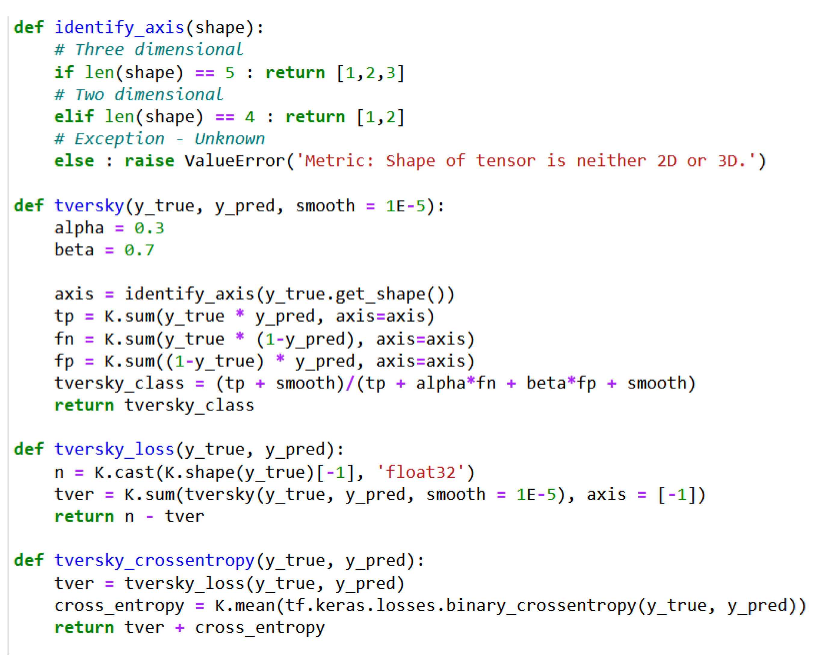
3.6. Hybrid U-Net Loss Function

Loss functions in machine learning help a model find an optimal solution. It takes the goal of minimizing the difference between the predictions and the ground truth. Typical types of loss functions in image segmentations include Jaccard loss, Dice loss, Binary Cross-Entropy (BCE) loss, and Binary Focal loss.

BCE loss is effective in measuring the difference between the actual and predicted image regions. However, the BCE loss depends on approximately equal data distribution. The effectiveness of BCE loss may become inadequate when a severe class imbalance exists, for example, the detection of small tumors in medical images.

Tversky focal loss can tackle the issue of class imbalance within the dataset [40]. As such, a customized loss function is designed in the proposed pipeline, that is, a hybrid Tversky–cross-entropy loss. It leverages the benefits of the BCE loss for strong convergence capability and the Tversky focal loss to handle the class imbalance. The implementation of the hybrid Tversky–cross-entropy loss function is shown in Figure 13.

3.7. Hybrid Optimizer for the U-Net in the Pipeline

Selecting a suitable optimizer (i.e., optimization algorithm) is crucial for effective backpropagation of the weight update in neural networks. The gradient descent optimizer utilizes a single-step movement (i.e., learning rate) for all neural nodes during the backpropagation, while the Adaptive Movement Estimation (Adam) optimizer uses different step sizes for different neural nodes, resulting in a quicker convergence. But the quick convergence can be hindered when the gradient becomes flat, resulting in convergence at local minima. In this case, the momentum can be incorporated to add inertia to the gradient descent process, which is known as Nesterov momentum. Thus, the Nadam optimization algorithm is able to achieve better optimization performance [41]. The Nadam optimizer is leveraged for the 3D U-Net in the proposed pipeline.

4. Experiment Results and Discussions

In the experiments, three different models of the 3D U-Net architecture in the pipeline are compared. The experiment results of each model are evaluated. The configurations of these three models are presented one by one.

4.1. Model 1 Configuration and Experiment Results

The 3D volume of each slice is divided into 225 cuboids. For Model 1, all cuboids per slice were used in the model training. Due to memory constraints, only the data from a small number of patients could be included in the model training. Model 1 is trained using the data of thirty-five patients and validated using the data of six patients. The configurations of the pipeline Model 1 are shown in

Table 5. Configurations of the pipeline Model 1.

Parameter	Value
Training Data	9450
Validation Data	1575
Train Array Size	7875 × 64 × 64 × 96 × 1
Validation Array Size	1350 × 64 × 64 × 96 × 1
Approximated Memory Usage	62.7 GB
Learning Rate at the Start	0.001
Optimizer	Nadam
Performance Metric	Dice coefficient
Activation Function	Sigmoid
Loss Function	hybrid Tversky-Cross Entropy loss
ReduceLROnPlateau	Factor: 0.1 Patience: 10
Batch Size	5
Epochs	300
Time used per epoch	1st Epoch: 265 s Subsequent Epochs: 250 s

.

The results of the Dice coefficient of Model 1 and its validation results are shown in Figure 14a, along with 300 epochs on the x-axis. The results of the loss metric of Model 1 are shown in Figure 14b.

For Model 1, the 2D prediction visualizations for the CT scans of two sample patients, patient 15 and patient 16, are displayed in Figure 15 and Figure 16, respectively. It can be seen that the prediction results are close to the ground truth masks.

For Model 1, the 3D volumetric prediction results for the scans of patients 15 and 16 are displayed in Figure 17 and Figure 18, respectively. High similarity can be observed between the masks and the prediction results, which demonstrates the good prediction performance of Model 1.

4.2. Model 2 Configuration and Experiment Results

In Model 2, only cuboids containing the mask label information were included in the training, while the background cuboids were removed. The total number of cuboids is significantly reduced in training, allowing for more patient data to fit into this model. Model 2 is trained using the data of 49 patients and validated using the data of 14 patients. The configurations of Model 2 are shown in

Table 6. Configurations of Model 2 in the experiment.

Parameter	Value
Training Data	1112
Validation Data	225
Train Array Size	1112 × 64 × 64 × 96 × 1
Validation Array Size	225 × 64 × 64 × 96 × 1
Approximated Memory Usage	25.5 GB
Learning Rate at the Start	0.0001
Optimizer	Nadam
Metric	Dice coefficient
Activation Function	Sigmoid
Loss Function	hybrid Tversky-Cross Entropy loss
ReduceLROnPlateau	Factor: 0.2 Patience: 7
Batch Size	4
Epochs	300
Time used per epoch	1st Epoch: 42 s Subsequent Epochs: 31 s

.

The results of the Dice coefficient of Model 2 and its validation results are shown in Figure 19a, along with 300 epochs of the x-axis. The results of the loss metric of Model 2 are shown in Figure 19b.

For Model 2, the 2D prediction visualizations for the CT scans of another two sample patients, patient 271 and patient 272, are displayed in Figure 20 and Figure 21, respectively. It is observed that the predicted results are close to the ground truth masks. But there are several false predictions in the results.

For Model 2, the 3D volumetric predictions for the CT scans of patients 271 and 272 are displayed in Figure 22 and Figure 23, respectively. A large number of false predictions are observed in the results. It could be caused by the total removal of the background cuboids in the model training.

4.3. Model 3 Configuration and Experiment Results

Model 3 was trained with a similar concept to Model 2. However, for every mask cuboid, an additional four (two front, two back) background cuboids were added to provide relevant context information for the model. Model 3 serves as a hybrid between Model 1 and Model 2. It utilizes less cuboids than Model 1, but more cuboids than Model 2. The configurations of Model 3 are shown in

Table 7. Configurations of Model 3 in the experiment.

Parameter	Value
Training Data	5560
Validation Data	1125
Train Array Size	5560 × 64 × 64 × 96 × 1
Validation Array Size	1125 × 64 × 64 × 96 × 1
Approximated Memory Usage	53.9 GB
Learning Rate at the Start	0.001
Optimizer	Nadam
Metric	Dice coefficient
Activation Function	Sigmoid
Loss Function	hybrid Tversky-Cross Entropy loss
ReduceLROnPlateau	Factor: 0.5 Patience: 8
Batch Size	5
Epochs	300
Time used per epoch	1st Epoch: 194 s Subsequent Epochs: 178 s

.

The results of the Dice coefficients of Model 3 and its validation results are shown in Figure 24a, along with 300 epochs on the x-axis. The results of the loss metric of Model 3 are shown in Figure 24b.

For Model 3, the 2D prediction visualizations for the CT scans of two sample patients, patient 271 and patient 272, are displayed in Figure 25 and Figure 26, respectively. A high similarity between the masks and predicted results is observed. There are no false predictions.

For Model 3, the 3D volumetric predictions for the CT scans of patients 271 and 272 are displayed in Figure 27 and Figure 28, respectively. While some false prediction results can be observed, it is an improvement from the results of Model 2.

4.4. Discussions and Comparisons of Three Models

For these three models presented in Section 4.1, Section 4.2 and Section 4.3, comparisons of the experiment results are shown in

Table 8. Brief comparisons of three models in the experiment.

Parameter	Model 1	Model 2	Model 3
Training Data	9450	1112	5560
Approximated Memory Usage	62.7 GB	25.5 GB	53.9 GB
Learning Rate at the Start	0.001	0.0001	0.001
ReduceLROnPlateau	Factor: 0.1 Patience: 10	Factor: 0.2 Patience: 7	Factor: 0.5 Patience: 8
Batch Size	5	4	5
Epochs	300	300	300
Time used for the 1st epoch (second)	265	42	194
Time used for subsequent epoch (second)	250	31	178
Dice Score on test data	91.44%	85.18%	89.84%

.

As seen from Table 8, even though Model 1 produces the highest Dice score at 91.44%, it utilizes the highest amount of memory and longest time compared to others.

Model 2 uses the least memory. The Dice score is at 85.18%, with many false predictions due to the removal of all background cuboids in the training data.

Model 3 provides a better balance between favorable predictions and memory usage. Model 3 is trained with cubes containing true masks and additional surrounding background cubes. This provides more background information to the model while preventing high memory usage compared to Model 1.

The prediction accuracies of Model 1–Model 3 in the pipeline are compared with three pre-trained models. The Segmentation Models (SMs) included in a high-level Python library with neural networks are available for image segmentation, where three pre-trained models, namely InceptionV3 [42], SM MobileNetV2 [43], and InceptionResNetV2 [44], were explored. The prediction accuracies of these models are shown in

Table 9. Comparisons of three models in the experiment with three pre-trained models and nine models reported in the literature.

Model	Dice Scores	Test Data Used for Experiments
Model 1	91.44%	Test data from this paper
Model 2	85.18%	Test data from this paper
Model 3	89.84%	Test data from this paper
InceptionV3 model [42]	91.20%	Pretrained model using test data from this paper
SM MobileNetV2 [43]	90.30%	Pretrained model using test data from this paper
InceptionResNetV2 [44]	88.10%	Pretrained model using test data from this paper
UCTransNet [32,45]	91.74%	SegPC 2021 cell segmentation dataset
	78.23%	Synapse multi-organ CT segmentation dataset
Attention U-Net [32,46]	91.58%	SegPC 2021 cell segmentation dataset
Multi Res-Unet [32,47]	86.94%	ISIC 2018 skin lesion segmentation dataset
TransUNet [32,48]	84.99%	ISIC 2018 skin lesion segmentation dataset
MISSFormer [32,49]	86.57%	ISIC 2018 skin lesion segmentation dataset
	81.96%	Synapse multi-organ CT segmentation dataset
Res-Unet [4,33]	89.4%	MRI dataset for breast cancer
U-Net [33,50]	80.2%	MRI dataset for breast cancer
Pipelined U-Net [33,51]	70.37%	MRI dataset for breast cancer
DenseNet [13]	94%	10-fold cross-validation for CT scan images

. It is observed that Model 1 in the pipeline performs better than the three pre-trained models.

Eight U-Net-based models [4,13,45,46,47,48] and one transformer-based model [49] reported in the literature were also compared with the proposed models in this paper. The Dice scores of these nine models are reported based on their own dataset, shown in Table 9. The Dice score is up to 91.74% for the SegPC 2021 cell segmentation dataset [45]. With the ISIC 2018 skin lesion segmentation dataset, the Dice score is up to 86.94% [47]. The Dice score is up to 81.96% for the Synapse multi-organ CT segmentation dataset [49]. Using an MRI dataset for breast cancer, the Dice score is up to 89.4% [4]. The Dice score is about 94%, obtained for CT scan images using a 10-fold cross-validation method, which is higher than that of the proposed Model 1 at 91.44%. The reason is that the 10-fold cross-validation approach is able to derive better accuracy of the segmentation.

5. Conclusions

An automatic tool for a volumetric prediction pipeline is developed for 3D CT scans on breast cancer in this paper. Various data pre-processing techniques are utilized to derive high-quality data to be fed into the model. Due to the nature of CT scans, not all data can be used directly without pre-processing. The developed pipeline consists of several algorithms to select suitable CT scan slices for the model training and test. The pipeline divides the 3D volumes into smaller segments to reduce the memory usage in the computation. It then conducts the normalization of 3D volumes and analyzes the depths of 3D CT scan slices.

Next, the data are fed into the 3D U-Net architecture in the pipeline. The 3D U-Net is designed to cater to the requirements of 3D image segmentation and volumetric prediction. Additional efforts are taken to perform optimization on memory usage and computation loads by reducing the number of training cuboids, and fine-tuning parameters in the U-Net model. A hybrid Tversky–cross-entropy loss function is employed in the pipeline. A Nadam optimization algorithm is utilized to derive favorable optimizer performance.

Three U-Net models with different configurations are implemented in this study. The performances of each model are discussed, with a few samples of prediction visualization illustrated. Among these three models, Model 3, which includes partial contextual information around the masked areas, obtains the most balanced performance on accuracy and memory usage for the CT scan image segmentation tasks. The experiment results are also compared with three pre-trained models, and nine models reported in the literature. Comparable Dice scores are achieved by the proposed pipeline in this paper.

Limitations and Future Works

There are two limitations for the model training performed in the current work. (1) CT scan slices with a thickness of 3 mm are utilized, and (2) only patient data with all masks in the range of the 1st–96th slices are utilized. With these two limitations, the amount of training data is reduced from 347 patients to approximately 50 patients. The essence of the machine learning model is that more training provides better generalization, which leads to better prediction on unseen data.

As future works, to tackle the first limitation, sampling can be performed on the data with CT scans of thicknesses of both 3 mm and 5 mm to increase the number of suitable input data. For the second limitation, a two-stage algorithm can be explored, where the volume segmentations on large cuboid dimensions will be conducted first, followed by breaking down a large cuboid into a certain number of cuboids in smaller dimensions. The volume segmentation can then be conducted on the small cuboids. Other types of loss functions and performance metrics can be explored as well. The k-fold cross-validation between models can be developed to further improve the accuracy of the model.

References

1. Anyoha, R. The History of Artificial Intelligence. 2017. Available online: https://sitn.hms.harvard.edu/flash/2017/history-artificial-intelligence/ (accessed on 10 November 2023).
2. Joksimovic, S.; Ifenthaler, D.; Marrone, R.; Laat, M.D.; Siemens, G. Opportunities of artificial intelligence for supporting complex problem-solving: Findings from a scoping review. Comput. Educ. Artif. Intell. 2023, 4, 100138. [Google Scholar] [CrossRef]
3. Zakaryan, V. How ML Will Disrupt the Future of Clinical Radiology. 2021. Available online: https://postindustria.com/computer-vision-in-radiology-how-ml-will-disrupt-the-future-of-clinical-radiology-healthcare/ (accessed on 10 November 2023).
4. Yue, W.; Zhang, H.; Zhou, J.; Li, G.; Tang, Z.; Sun, Z.; Cai, J.; Tian, N.; Gao, S.; Dong, J.; et al. Deep learning-based automatic segmentation for size and volumetric measurement of breast cancer on magnetic resonance imaging. Front. Oncol. 2022, 12, 984626. [Google Scholar] [CrossRef] [PubMed]
5. Jafari, Z.; Karami, E. Breast Cancer Detection in Mammography Images: A CNN-Based Approach with Feature Selection. Information 2023, 14, 410. [Google Scholar] [CrossRef]
6. Liu, Z.; Liu, F.; Chen, W.; Liu, X.; Hou, X.; Shen, J.; Guan, H.; Zhen, H.; Wang, S.; Chen, Q.; et al. Automatic Segmentation of Clinical Target Volumes for Post-Modified Radical Mastectomy Radiotherapy Using Convolutional Neural Networks. Front. Oncol. 2021, 10, 581347. [Google Scholar] [CrossRef]
7. Gaudez, S.; Slama, M.B.H.; Kaestner, A.; Upadhyay, M.V. 3D deep convolutional neural network segmentation model for precipitate and porosity identification in synchrotron X-ray tomograms. J. Synchrotron Radiat. 2022, 29, 1232–1240. [Google Scholar] [CrossRef]
8. Xie, L.; Liu, Z.; Pei, C.; Liu, X.; Cui, Y.-Y.; He, N.-A.; Hu, L. Convolutional neural network based on automatic segmentation of peritumoral shear-wave elastography images for predicting breast cancer. Front. Oncol. 2023, 13, 1099650. [Google Scholar] [CrossRef]
9. Zhang, Y.; Chan, S.; Park, V.Y.; Chang, K.-T.; Mehta, S.; Kim, M.J.; Combs, F.J.; Chang, P.; Chow, D.; Parajuli, R.; et al. Automatic Detection and Segmentation of Breast Cancer on MRI Using Mask R-CNN Trained on Non–Fat-Sat Images and Tested on Fat-Sat Images. Acad. Radiol. 2020, 29, S135–S144. [Google Scholar] [CrossRef]
10. Raimundo, J.N.C.; Fontes, J.P.P.; Magalhães, L.G.M.; Lopez, M.A.G. An Innovative Faster R-CNN-Based Framework for Breast Cancer Detection in MRI. J. Imaging 2023, 9, 169. [Google Scholar] [CrossRef] [PubMed]
11. Qi, T.H.; Hian, O.H.; Kumaran, A.M.; Tan, T.J.; Cong, T.R.Y.; Su-Xin, G.L.; Lim, E.H.; Ng, R.; Yeo, M.C.R.; Tching, F.L.L.W. Multi-center evaluation of artificial intelligent imaging and clinical models for predicting neoadjuvant chemotherapy response in breast cancer. Breast Cancer Res. Treat. 2022, 193, 121–138. [Google Scholar] [CrossRef]
12. Buelens, P.; Willems, S.; Vandewinckele, L.; Crijns, W.; Maes, F.; Weltens, C. Clinical evaluation of a deep learning model for segmentation of target volumes in breast cancer radiotherapy. Radiother. Oncol. 2022, 171, 84–90. [Google Scholar] [CrossRef]
13. Sreenivasu, S.V.N.; Gomathi, S.; Kumar, M.J.; Prathap, L.; Madduri, A.; Almutairi, K.M.A.; Alonazi, W.B.; Kali, D.; Jayadhas, S.A. Dense Convolutional Neural Network for Detection of Cancer from CT Images. BioMed Res. Int. 2022, 2022, 1293548. [Google Scholar] [CrossRef]
14. Shehmir, J. Computer Vision in Radiology: Benefits & Challenges. 19 July 2022. Available online: https://research.aimultiple.com/computer-vision-radiology (accessed on 11 November 2023).
15. Esteva, A.; Chou, K.; Yeung, S.; Naik, N.; Madani, A.; Mottaghi, A.; Liu, Y.; Topol, E.; Dean, J.; Socher, R. Deep learning-enabled medical computer vision. NPJ Digit. Med. 2021, 4, 5. [Google Scholar] [CrossRef] [PubMed]
16. Costa, M.G.F.; Campos, J.P.M.; Aquino, G.d.A.e.; Pereira, W.C.d.A.; Filho, C.F.F.C. Evaluating the performance of convolutional neural networks with direct acyclic graph architectures in automatic segmentation of breast lesion in US images. BMC Med. Imaging 2019, 19, 85. [Google Scholar] [CrossRef]
17. Al Bataineh, A.; Kaur, D.; Al-Khassaweneh, M.; Al-Sharoa, E. Automated CNN Architectural Design: A Simple and Efficient Methodology for Computer Vision Tasks. Mathematics 2023, 11, 1141. [Google Scholar] [CrossRef]
18. Taye, M.M. Theoretical Understanding of Convolutional Neural Network: Concepts, Architectures, Applications, Future Directions. Computation 2023, 11, 52. [Google Scholar] [CrossRef]
19. Soffer, S.; Ben-Cohen, A.; Shimon, O.; Amitai, M.M.; Greenspan, H.; Klang, E. Convolutional Neural Networks for Radiologic Images: A Radiologist’s Guide. Radiology 2019, 290, 590–606. [Google Scholar] [CrossRef]
20. Lecun, Y.; Bottou, L.; Bengio, Y.; Haffner, P. Gradient-based learning applied to document recognition. Proc. IEEE 1998, 86, 2278–2324. [Google Scholar] [CrossRef]
21. Rosebrock, A. LeNet: Recognizing Handwritten Digits. 22 May 2021. Available online: https://pyimagesearch.com/2021/05/22/lenet-recognizing-handwritten-digits/ (accessed on 8 November 2023).
22. Krizhevsky, A.; Sutskever, I.; Hinton, G.E. Imagenet classification with deep convolutional neural networks. Commun. ACM 2017, 60, 84–90. [Google Scholar] [CrossRef]
23. Han, X.; Zhong, Y.; Cao, L.; Zhang, L. Pre-Trained AlexNet Architecture with Pyramid Pooling and Supervision for High Spatial Resolution Remote Sensing Image Scene Classification. Remote Sens. 2017, 9, 848. [Google Scholar] [CrossRef]
24. Zeiler, M.D.; Fergus, R. Visualizing and Understanding Convolutional Networks. In Computer Vision—ECCV 2014. ECCV 2014; Fleet, D., Pajdla, T., Schiele, B., Tuytelaars, T., Eds.; Lecture Notes in Computer Science; Springer: Cham, Switzerland, 2014; Volume 8689. [Google Scholar] [CrossRef]
25. Abdelhafiz, D.; Yang, C.; Ammar, R.; Nabavi, S. Deep convolutional neural networks for mammography: Advances, challenges and applications. BMC Bioinform. 2019, 20, 281. [Google Scholar] [CrossRef]
26. Szegedy, C.; Liu, W.; Jia, Y.; Sermanet, P.; Reed, S.; Anguelov, D.; Erhan, D.; Vanhoucke, V.; Rabinovich, A.; Liu, W.; et al. Going deeper with convolutions. In Proceedings of the IEEE Conference on Computer Vision and Pattern Recognition (CVPR) 2015, Boston, MA, USA, 7–12 June 2015; pp. 1–9. [Google Scholar] [CrossRef]
27. Simonyan, K.; Zisserman, A. Very Deep Convolutional Networks for Large-Scale Image Recognition. arXiv 2014, arXiv:1409.1556. [Google Scholar]
28. He, K.; Zhang, X.; Ren, S.; Sun, J. Deep residual learning for image recognition. In Proceedings of the IEEE Conference on Computer Vision and Pattern Recognition, Las Vegas, NV, USA, 26 June–1 July 2016; pp. 770–778. [Google Scholar]
29. Howard, A.G.; Zhu, M.; Chen, B.; Kalenichenko, D.; Wang, W.; Weyand, T.; Andreetto, M.; Adam, H. MobileNets: Efficient Convolutional Neural Networks for Mobile Vision Applications. arXiv 2017, arXiv:1704.04861. [Google Scholar] [CrossRef]
30. Ronneberger, O.; Fischer, P.; Brox, T. U-Net: Convolutional Networks for Biomedical Image Segmentation. In Medical Image Computing and Computer-Assisted Intervention—MICCAI 2015. MICCAI 2015; Navab, N., Hornegger, J., Wells, W., Frangi, A., Eds.; Lecture Notes in Computer Science; Springer: Cham, Switzerland, 2015; Volume 9351. [Google Scholar] [CrossRef]
31. Zhang, J. Unet—Line by Line Explanation. 18 October 2019. Available online: https://towardsdatascience.com/unet-line-by-line-explanation-9b191c76baf5 (accessed on 10 November 2023).
32. Azad, R.; Aghdam, E.K.; Rauland, A.; Jia, Y.; Avval, A.H.; Bozorgpour, A.; Karimijafarbigloo, S.; Cohen, J.P.; Adeli, E.; Merhof, D. Medical Image Segmentation Review: The Success of U-net. arXiv 2022, arXiv:2211.14830. [Google Scholar] [CrossRef]
33. Luo, L.; Wang, X.; Lin, Y.; Ma, X.; Tan, A.; Chan, R.; Vardhanabhuti, V.; Chu, W.C.; Cheng, K.-T.; Chen, H. Deep Learning in Breast Cancer Imaging: A Decade of Progress and Future Directions. arXiv 2024, arXiv:2304.06662. [Google Scholar] [CrossRef] [PubMed]
34. Kodipalli, A.; Fernandes, S.L.; Gururaj, V.; Rameshbabu, S.V.; Dasar, S. Performance Analysis of Segmentation and Classification of CT-Scanned Ovarian Tumours Using U-Net and Deep Convolutional Neural Networks. Diagnostics 2023, 13, 2282. [Google Scholar] [CrossRef] [PubMed]
35. Sakshi; Kukreja, V. Image Segmentation Techniques: Statistical, Comprehensive, Semi-Automated Analysis and an Application Perspective Analysis of Mathematical Expressions. Arch. Comput. Methods Eng. 2022, 30, 457–495. [Google Scholar] [CrossRef]
36. Barrowclough, O.J.; Muntingh, G.; Nainamalai, V.; Stangeby, I. Binary segmentation of medical images using implicit spline representations and deep learning. Comput. Aided Geom. Des. 2021, 85, 101972. [Google Scholar] [CrossRef]
37. Qian, Q.; Cheng, K.; Qian, W.; Deng, Q.; Wang, Y. Image Segmentation Using Active Contours with Hessian-Based Gradient Vector Flow External Force. Sensors 2022, 22, 4956. [Google Scholar] [CrossRef] [PubMed]
38. Yu, Y.; Wang, C.; Fu, Q.; Kou, R.; Huang, F.; Yang, B.; Yang, T.; Gao, M. Techniques and Challenges of Image Segmentation: A Review. Electronics 2023, 12, 1199. [Google Scholar] [CrossRef]
39. Huo, Y.; Tang, Y.; Chen, Y.; Gao, D.; Han, S.; Bao, S.; De, S.; Terry, J.G.; Carr, J.J.; Abramson, R.G.; et al. Stochastic tissue window normalization of deep learning on computed tomography. J. Med. Imaging 2019, 6, 044005. [Google Scholar] [CrossRef]
40. Abraham, N.; Khan, N.M. A Novel Focal Tversky Loss Function with Improved Attention U-Net for Lesion Segmentation. In Proceedings of the 2019 IEEE 16th International Symposium on Biomedical Imaging (ISBI 2019), Venice, Italy, 8–11 April 2019; pp. 683–687. [Google Scholar] [CrossRef]
41. Haji, S.H.; Abdulazeez, A.M. Comparison of optimization techniques based on gradient descent algorithm: A review. Palarch’s J. Archaeol. Egypt/Egyptol. 2021, 18, 2715–2743. [Google Scholar]
42. TensorFlow. tf.keras.applications.inception_v3.InceptionV3. Available online: https://www.tensorflow.org/api_docs/python/tf/keras/applications/inception_v3/InceptionV3 (accessed on 15 January 2024).
43. Keras. MobileNet, MobileNetV2, and MobileNetV3. Available online: https://keras.io/api/applications/mobilenet/ (accessed on 25 January 2024).
44. TensorFlow. tf.keras.applications.inception_resnet_v2.InceptionResNetV2. Available online: https://www.tensorflow.org/api_docs/python/tf/keras/applications/inception_resnet_v2/InceptionResNetV2 (accessed on 25 January 2024).
45. Wang, H.; Cao, P.; Wang, J.; Zaiane, O.R. UCTransNet: Rethinking the skip connections in u-net from a channel-wise perspective with transformer. Proc. AAAI Conf. Artif. Intell. 2022, 36, 2441–2449. [Google Scholar] [CrossRef]
46. Oktay, O.; Schlemper, J.; Le Folgoc, L.; Lee, M.; Heinrich, M.; Misawa, K.; Mori, K.; McDonagh, S.; Hammerla, N.Y.; Kainz, B. Attention U-Net: Learning Where to Look for the Pancreas. arXiv 2018, arXiv:1804.03999. [Google Scholar]
47. Ibtehaz, N.; Rahman, M.S. MultiResUNet: Rethinking the U-Net architecture for multimodal biomedical image segmentation. Neural Netw. 2020, 121, 74–87. [Google Scholar] [CrossRef] [PubMed]
48. Chen, J.; Lu, Y.; Yu, Q.; Luo, X.; Adeli, E.; Wang, Y.; Lu, L.; Yuille, A.L.; Zhou, Y. TransUNet: Transformers Make Strong Encoders for Medical Image Segmentation. arXiv 2021, arXiv:2102.04306. [Google Scholar]
49. Huang, X.; Deng, Z.; Li, D.; Yuan, X. Missformer: An Effective Medical Image Segmentation Transformer. arXiv 2021, arXiv:2109.07162. [Google Scholar] [CrossRef]
50. Khaled, R.; Vidal, J.; Vilanova, J.C.; Martí, R. A U-Net Ensemble for breast lesion segmentation in DCE MRI. Comput. Biol. Med. 2021, 140, 105093. [Google Scholar] [CrossRef]
51. Galli, A.; Marrone, S.; Piantadosi, G.; Sansone, M.; Sansone, C. A Pipelined Tracer-Aware Approach for Lesion Segmentation in Breast DCE-MRI. J. Imaging 2021, 7, 276. [Google Scholar] [CrossRef]
Figure 1. Anisotropic CT scans of patients.
Mathematics 12 00616 g001
Figure 2. Structure of the proposed prediction pipeline.
Mathematics 12 00616 g002
Figure 3. Flow chart to extract number of slices per patient in the axial plane.
Mathematics 12 00616 g003
Figure 4. Output of extracted number of slices per patient.
Mathematics 12 00616 g004
Figure 5. Flow chart to record the slice indexes with the presence of masks.
Mathematics 12 00616 g005
Figure 6. Sample outputs indicate the patient slices with the presence of masks.
Mathematics 12 00616 g006
Figure 7. Flow chart to classify patients according to the indexes of mask slice presence.
Mathematics 12 00616 g007
Figure 8. Patient pixel matrix illustration.
Mathematics 12 00616 g008
Figure 9. Segmented 3D volume using Patchify library. The segmented cuboids are shown in red boxes.
Mathematics 12 00616 g009
Figure 10. Flow chart to voxelize training data.
Mathematics 12 00616 g010
Figure 11. Three-dimensional U-Net architecture developed in the proposed pipeline.
Mathematics 12 00616 g011
Figure 12. The code implementation of the 3D U-Net in the pipeline.
Mathematics 12 00616 g012
Figure 13. Implementation of the hybrid Tversky–cross-entropy loss function.
Mathematics 12 00616 g013
Figure 14. Performance and loss function results of Model 1. (a) The Dice coefficients in the training (blue) and validation (orange). (b) The loss metrics in the training (blue) and validation (orange).
Mathematics 12 00616 g014
Figure 15. Two-dimensional prediction result for patient 15 in Model 1. From left to right: scans, masks, and predictions, respectively.
Mathematics 12 00616 g015
Figure 16. Two-dimensional prediction result for patient 16 in Model 1. From left to right: scans, masks, and predictions, respectively.
Mathematics 12 00616 g016
Figure 17. Three-dimensional volumetric predictions for patient 15 in Model 1.
Mathematics 12 00616 g017aMathematics 12 00616 g017b
Figure 18. Three-dimensional volumetric predictions for patient 16 in Model 1.
Mathematics 12 00616 g018
Figure 19. Performance and loss function results of Model 2. (a) The Dice coefficients in the training (blue) and validation (orange). (b) The loss metrics in the training (blue) and validation (orange).
Mathematics 12 00616 g019
Figure 20. Prediction results for patient 271 of Model 2. From left to right: scans, masks, and prediction results.
Mathematics 12 00616 g020
Figure 21. Prediction results for patient 272 of Model 2. From left to right: scans, masks, and prediction results.
Mathematics 12 00616 g021
Figure 22. Three-dimensional volumetric predictions for patient 271 in Model 2.
Mathematics 12 00616 g022aMathematics 12 00616 g022b
Figure 23. Three-dimensional volumetric predictions for patient 272 in Model 2.
Mathematics 12 00616 g023
Figure 24. Performance and loss function results of Model 3. (a) The Dice coefficients in the training (blue) and validation (orange). (b) The loss metrics in the training (blue) and validation (orange).
Mathematics 12 00616 g024
Figure 25. Prediction results for patient 271 of Model 3. From left to right: scans, masks, and prediction results.
Mathematics 12 00616 g025
Figure 26. Prediction results for patient 272 of Model 3. From left to right: scans, masks, and prediction results.
Mathematics 12 00616 g026
Figure 27. Three-dimensional volumetric predictions for patient 271 in Model 3.
Mathematics 12 00616 g027aMathematics 12 00616 g027b
Figure 28. Three-dimensional volumetric predictions for patient 272 in Model 3.
Mathematics 12 00616 g028