Finite-Time Robust Path-Following Control of Perturbed Autonomous Ground Vehicles Using a Novel Self-Tuning Nonsingular Fast Terminal Sliding Manifold

Abstract

This work presents a finite-time robust path-following control scheme for perturbed autonomous ground vehicles. Specifically, a novel self-tuning nonsingular fast-terminal sliding manifold that further enhances the convergence rate and tracking accuracy is proposed. Then, uncertain dynamics and external disturbances are estimated by a high-gain disturbance observer to compensate for the designed control input. Successively, a super-twisting algorithm is incorporated into the final control law, significantly mitigating the chattering phenomenon of both the input control signal and the output trajectory. Furthermore, the global finite-time convergence and stability of the whole proposed control algorithm are proven by the Lyapunov theory. Finally, the efficacy of the proposed method is validated with comparisons in a numerical example. It obtains high control performance, reduced chattering, fast convergence rate, singularity avoidance, and robustness against uncertainties.

1. Introduction

With the lightning speed of advances in artificial intelligence, smart cities, self-driving vehicles, robots, and others, autonomous ground vehicles (AGV) as intelligent mobile robots have been widely applied to various fields [1]. They play an essential role in both domestic and industrial applications to enhance safety and efficiency requirements. Thus, control for path following has always been a topic of significant interest in the AGV field, which garners a great deal of attention from numerous researchers [2]. In path following, position and orientation errors are handled through several approaches [3,4]. Although their effectiveness was proven to bring good performance, the system stability is hardly considered [5], and it is quite complex to consider a multi-input–multi-output nonlinear system [6,7,8]. Fortunately, the control design process for path following can be simplified with the assistance of the Lyapunov function [9]. It not only can reach high precision but also guarantees system stability in terms of the control principle.

The well-known sliding-mode control (SMC) framework has been considered as one of the most promising candidates for robust controller designs, as it can attenuate the influences of uncertainties/disturbances thoroughly, such as a fractional-order SMC [10] or coupled adaptive rule in SMC [11,12]. Basically, the design structure consists of the reaching phase and sliding phase. The reaching phase drives state variables toward the sliding surface, which deals with the lumped uncertainty of the system. After that, the state variables are driven toward the origin point along the sliding surface in the sliding phase, which guarantees the convergence property of the controller. It is noteworthy that the key idea in the SMC is the finite-time convergence of the system states to a pre-designed sliding surface in its state space and then maintaining the system trajectory on this surface for all future times. This is achieved through the application of a discontinuous control action that switches between different states, ensuring that the system can counteract any disturbances or uncertainties and follow the desired trajectory closely. However, the state trajectory is hard to converge toward the origin point in a finite time due to the linear sliding surface. Thus, finite-time convergence of the sliding phase is a key challenge. With regard to this issue, the nonlinear sliding surface is developed, namely a terminal sliding mode control (TSMC) [13]. This sliding surface is designed to guide the sliding variables of the system toward the equilibrium point within a finite time span, ensuring fast convergence. To further enhance the convergence speed and overcome the slow convergence problem, a fast TSMC (FTSMC) is introduced in [14,15]. The FTSMC builds upon the TSMC concept [16] and provides an improved control scheme to achieve quicker and more efficient convergence for the system. Moreover, when the sliding variable is approximately zero, it obeys the TSMC working principle and the finite-time convergence is ensured. Inherently, the FTSMC still suffers from the singularity problem of the TSMC, which is a major limitation of the SMC design. To overcome the limitation, a nonsingular FTSMC (NFTSMC) is proposed in [17]. It aims to upgrade the FTSMC to a new version that avoids singularity issues. Nonetheless, the sliding surface gains of the NFTSMC may remain fixed, lowering the convergence rate of the state variables in the sliding phase. Hence, an adaptive NFTSMC (ANFTSMC) [18,19] is proposed to solve the fixed-gain shortcoming. However, the singularity caused by the negative fractional power on this sliding surface has not yet been thoroughly addressed.

On the other hand, the chattering phenomenon is a common issue in sliding-mode control systems due to the high-frequency switching of the control input [20,21]. This happens due to the inherent switching nature of the SMC algorithm caused by using the signum function, which continuously toggles the control input between two states to keep the system’s state on the desired sliding surface. While effective for maintaining robust control in the presence of disturbances and uncertainties, this incessant switching can lead to significant noise generation, which degrades the control performance as well as wear on actuators in practical systems. To address this problem, the boundary layer (BL) method has been introduced, replacing the signum function with sigmoid [22] or saturation functions [23]. The BL method imposes bounds on the control output, striking a balance between control smoothness and system robustness. Despite the effectiveness, unavoidable trade-offs are created between these two aspects. An alternative approach to enhance both robustness and control smoothness is the super-twisting algorithm (STW) [24,25]. This algorithm ensures finite-time establishment of the sliding mode, leading to improved robustness and smoother control output simultaneously. Additionally, reducing the control gain during the reaching phase is seen as a promising solution. This can be achieved through the use of fuzzy logic systems (FLS) and neural networks (NNs) [26]. These techniques can dynamically adjust the control gain based on system conditions, contributing to improved control performance and reduced chattering effects. Nevertheless, these methods require expert knowledge or training processes for approximating the unknown system dynamics, which is unsuitable for dealing with external disturbances. Meanwhile, the disturbance observer (DO) technique is a robust approach commonly used for estimating both uncertainties and external disturbances [27,28]. Moreover, the estimated uncertainties and disturbances in the system can be compensated, improving the robustness of the control system.

Inspired by the above-mentioned problems, this paper proposes a new finite-time robust control framework for the path-following of the perturbed AGVs. Simultaneously, we integrate both a high-gain disturbance observer (HGDO) and a super-twisting algorithm (STW) to not only reduce chattering but also increase control accuracy. The key points of this work are summarized as follows:

• The novel self-tuning nonsingular fast terminal sliding manifold (SNFTSM) for a robust control design is proposed; it delivers a closed-loop control with a fast convergence rate, singularity avoidance, and high performance of the output against uncertain terms.
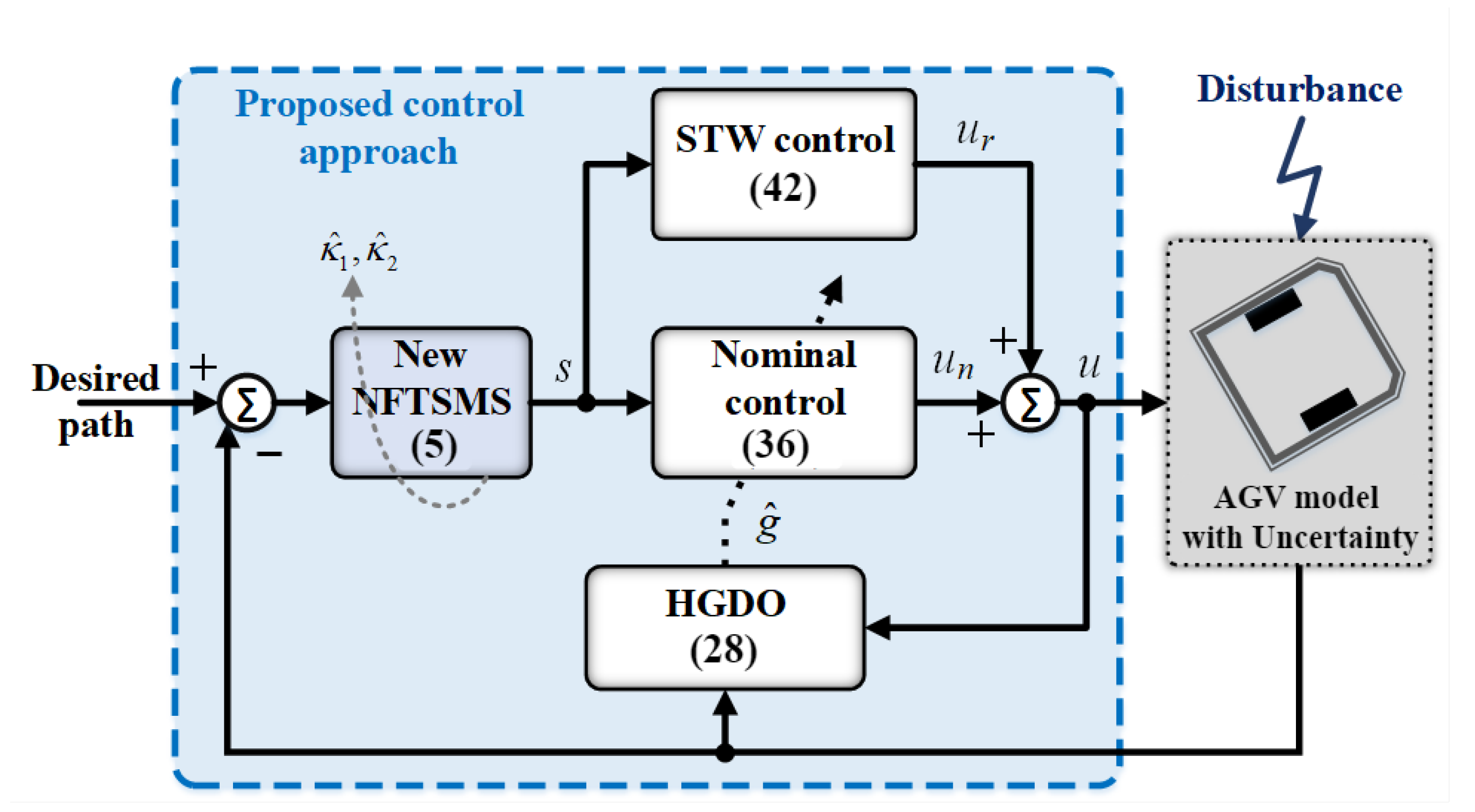
• The proposed control framework based on the novel SNFTSM is integrated with the HGDO technique and the STW to simultaneously obtain great tracking performance and successfully mitigate chattering phenomena.
• A rigorous analysis is provided to theoretically prove the global finite-time convergence and stability of the whole closed-loop system in both phases. Moreover, the performance of the control approach in the presence of uncertainties and disturbances is confirmed.

The remaining sections of the paper are structured as follows: Section 2 provides the problem formulation. Section 3 describes the proposed control method, detailing its components and implementation. Results with the numerical example are discussed in Section 4. Finally, the conclusions are given in Section 5.

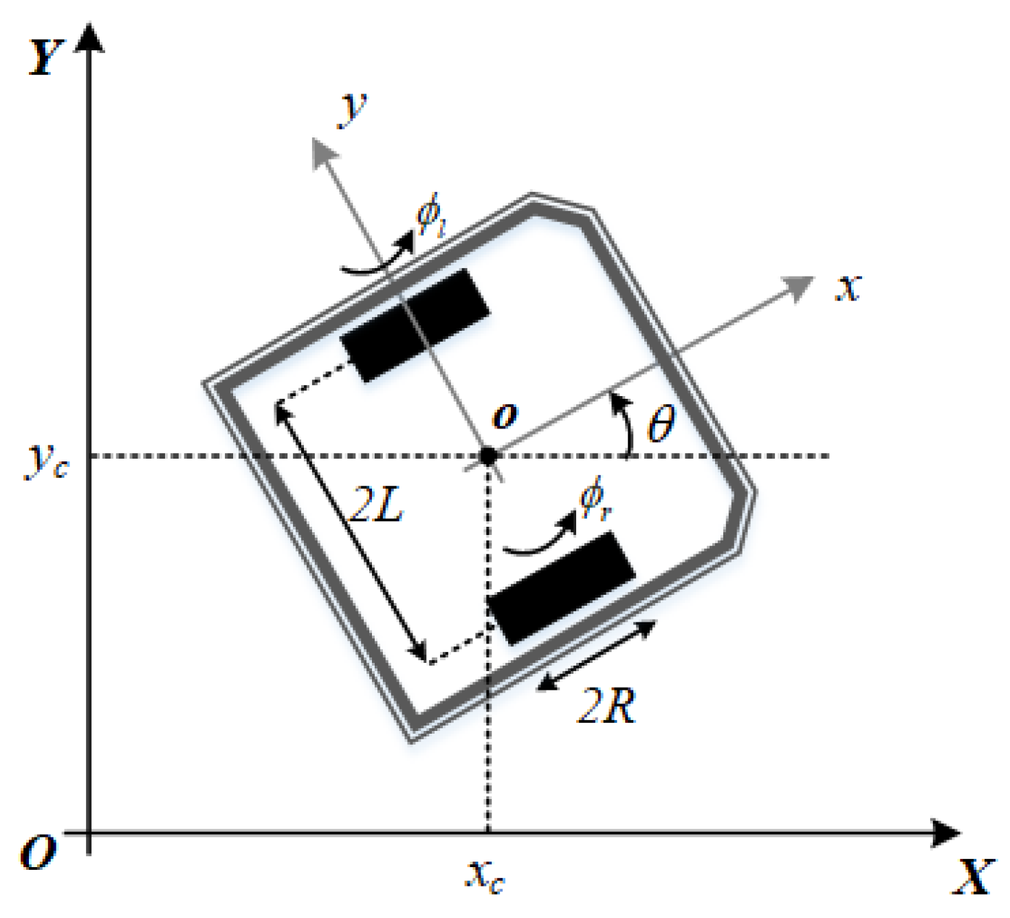
2. Problem Formulation

General robot dynamics can be described by the equation of motion as the following.

$$\begin{array}{cc}\hfill M\left(q\right)\ddot{q}& +V(q,\dot{q})\dot{q}+{\mathrm{\Lambda }}^{\top }\left(q\right)\lambda +{\Delta }_d(q,\dot{q})=B\left(q\right)u\hfill \end{array}$$

(1)

where q, $\dot{q}$, and $\ddot{q}\in {\mathbb{R}}^{n\times 1}$ denote the position, velocity, and the acceleration, respectively; u denotes the control input vectors; $M\left(q\right)\in {\mathbb{R}}^{n\times n}$ is a symmetric positive definite inertia matrix; $V(q,\dot{q})\in {\mathbb{R}}^{n\times n}$ is the centripetal and Coriolis matrix; $B\left(q\right)\in \mathbb{R}$ is the input matrix; $\mathrm{\Lambda }\left(q\right)$ is the matrix associated with the kinematic constraints with Lagrange multipliers $\lambda$ [29]; ${\Delta }_d=T_d+f_c$ is the vector of bounded unknown disturbances $T_d$ and the surface friction $f_c$.

To simplify the dynamic model, (1) can be presented as

$$\begin{array}{c}\hfill \ddot{q}=M^{-1}\left(q\right)(B\left(q\right)u+f(q,\dot{q})+g(t,q,\dot{q}))\end{array}$$

(2)

where $f(q,\dot{q})=-M^{-1}\left(q\right)V(q,\dot{q})\dot{q}$ and $g(t,q,\dot{q})=-M^{-1}\left(q\right)({\mathrm{\Lambda }}^{\top }\left(q\right)$$\lambda$$+{\Delta }_d(q,\dot{q}))$ denote the nominal term and the lumped disturbance and uncertainty terms in the system, respectively.

Assumption 1.

According to [4,30,31,32], suppose that the lumped disturbance g and its derivative $\dot{g}$ are differentiable and bounded.

$$∥g(t,q,\dot{q})∥\le {\delta }_g$$

(3)

$$∥\dot{g}(t,q,\dot{q})∥\le {\delta }_{\dot{g}}$$

(4)

where ${\delta }_g$ and ${\delta }_{\dot{g}}$ are positive constants.

3. The Proposed Control Approach

In this section, we present the design of a novel SNFTSM that aims to enhance fast-tracking accuracy within a finite time frame. Building upon this advancement, we introduce a new finite-time robust control scheme that integrates both the HGDO technique and the STW. The structure of the proposed controller is illustrated in Figure 1.

3.1. Design of a Novel SNFTSM

To obtain a fast finite-time convergence and singularity avoidance of the terminal sliding mode surface, a novel SNFTSM is proposed as follows:

$$\begin{array}{c}\hfill s={\dot{q_e}}^{\upsilon }+{\widehat{\kappa }}_1{q}_e^{\upsilon \gamma }+{\widehat{\kappa }}_2{q}_e\end{array}$$

(5)

where $q_e=q_d-q$ and ${\dot{q}}_e={\dot{q}}_d-\dot{q}$ are the differential values between the output signal and the desired signal. Herein, $q_d$ and ${\dot{q}}_d$ represent the desired trajectory and its time derivative, respectively. To ensure generality, we introduce the parameter $v=m_v/n_v$, where $m_v$ and $n_v$ are consecutive positive odd numbers satisfying $1<v<2$. Furthermore, the sliding surface incorporates an additional positive odd number $\gamma$ to enhance its versatility. The self-tuning gains for the fast and terminal terms of the sliding surface are denoted as ${\widehat{\kappa }}_1$ and ${\widehat{\kappa }}_2$, respectively, and their design is expressed as follows:

$${\widehat{\kappa }}_1=k_1{\mathbf{e}}^{{\eta }_1(q_e^{\alpha }-{\mu }^{\alpha })}$$

(6)

$${\widehat{\kappa }}_2=k_2{\mathbf{e}}^{-{\eta }_2(q_e^{\beta }-{\mu }^{\beta })}$$

(7)

where $\mathbf{e}$ represents the exponential function; $k_1$, $k_2$, ${\eta }_1$, and ${\eta }_2$ are positive values; $\alpha ,\beta$ are the integer constant values to adjust the convergence rate; and $\mu =\pm {(k_1/k_2)}^{1/(1-v\gamma )}$.

Remark 1.

It can be seen that the initial point at any position in the state space can approach the sliding phase in finite time. Owing to the exponential function, the magnitude of ${\widehat{\kappa }}_1$ (6) and ${\widehat{\kappa }}_2$ (7) are changeable values and inverse to each other depending on the system error. Thus the reaching law can be self-adjusted; it enhances faster convergence time of reaching motion.

Theorem 1.

The proposed SNFTSM (5) guarantees fast convergence from the initial point $q_e\left(0\right)$ to μ and from μ to the origin (i.e., zero) in a finite time for the state error in the sliding phase.

Proof. 

When the system error moves to the sliding phase, the sliding surface becomes ${\dot{q_e}}^{\upsilon }+{\widehat{\kappa }}_1{q}_e^{\upsilon \gamma }+{\widehat{\kappa }}_2{q}_e=0$. Then $\dot{q_e}={\left(-{\widehat{\kappa }}_1{q}_e^{\upsilon \gamma }-{\widehat{\kappa }}_2{q}_e\right)}^{1/v}$. To prove Theorem 1, the Lyapunov candidate function is selected as follows:

$$\begin{array}{c}\hfill V_1=\frac{1}{2}{q}_e^2\end{array}$$

(8)

The time derivative of $V_1$ can be given as

$$\begin{array}{cc}\hfill {\dot{V}}_1& =q_e{\dot{q}}_e\hfill \\ \hfill & ={\left(-{\widehat{\kappa }}_1{q}_e^{\upsilon (\gamma +1)}-{\widehat{\kappa }}_2{q}_e^{v+1}\right)}^{1/v}\hfill \end{array}$$

(9)

When the initial position of error is far from the origin $(q_e\left(0\right)>\mu )$, thanks to the unique feature of the new manifold (see Remark 1), the fast term containing ${\widehat{\kappa }}_1^v{q}_e^{v\gamma }$ strongly suppresses the terminal term ${\widehat{\kappa }}_2^v{q}_e^{v+1}$. Then, (9) becomes the expression as follows:

$$\begin{array}{cc}\hfill {\dot{V}}_1& ={\left(-{\widehat{\kappa }}_1{q}_e^{\upsilon (\gamma +1)}-{\widehat{\kappa }}_2{q}_e^{v+1}\right)}^{1/v}\hfill \\ \hfill & \le {\left(-{\widehat{\kappa }}_1{q}_e^{\upsilon (\gamma +1)}\right)}^{1/v}\hfill \\ \hfill & \le {\left(-k_1{q}_e^{\upsilon (\gamma +1)}\right)}^{1/v}\hfill \\ \hfill & \le -k_1^{1/v}{V}_1^{(\gamma +1)/2}\hfill \end{array}$$

(10)

Taking the integral for both sides of (10) with respect to time yields the following result:

$$\begin{array}{c}\hfill {\int }_{V_1\left(q_e\left(0\right)\right)}^{V_1\left(\mu \right)}{V}_1^{-(\gamma +1)/2}d{V}_1\le {\int }_0^{t_1}-k_1^{1/v}\mathrm{d}t\end{array}$$

(11)

where $V_1\left(q_e\left(0\right)\right)=\frac{1}{2}{\left(q_e\left(0\right)\right)}^2$ and $V_1\left(\mu \right)=\frac{1}{2}{\left(\mu \right)}^2$.

The result from solving Equation (11) is expressed as

$$\begin{array}{cc}\hfill t_1& \le \frac{2V_1{\left(q_e\left(0\right)\right)}^{(1-\gamma )/2}}{(1-\gamma )k_1^{1/v}}-\frac{2V_1{\left(\mu \right)}^{(1-\gamma )/2}}{(1-\gamma )k_1^{1/v}}\hfill \\ \hfill & \le \frac{2^{(1+\gamma )/2}{q}_e{\left(0\right)}^{1-\gamma }}{(1-\gamma )k_1^{1/v}}-\frac{2^{(1+\gamma )/2}{\mu }^{1-\gamma }}{(1-\gamma )k_1^{1/v}}\hfill \end{array}$$

(12)

Based on (12), the proposed control approach achieves a reduction in the control error from the initial position $q_e\left(0\right)$ to $\mu$ within a finite time. As the system state approaches the equilibrium point ($|q_e|<|\mu |$), the term ${\widehat{\kappa }}_2{q}_e^{v+1}$ dominates over ${\widehat{\kappa }}_1{q}_e^{v\gamma }$, ensuring finite-time convergence of the SNFTSM (5). The time derivative of the Lyapunov function (9) can be expressed as follows:

$$\begin{array}{cc}\hfill {\dot{V}}_1& ={\left(-{\widehat{\kappa }}_1{q}_e^{\upsilon (\gamma +1)}-{\widehat{\kappa }}_2{q}_e^{v+1}\right)}^{1/v}\hfill \\ & \le {\left(-{\widehat{\kappa }}_2{q}_e^{v+1}\right)}^{1/v}\hfill \\ \hfill & \le {\left(-k_2{q}_e^{v+1}\right)}^{1/v}\hfill \\ & \le -k_2^{1/v}{V}_1^{(v+1)/\left(2v\right)}\hfill \end{array}$$

(13)

This expression demonstrates the effectiveness of the suggested strategy in achieving finite-time convergence of the system error and ensuring stability near the equilibrium point. Taking the integral for both sides of (13) with respect to time yields the following.

$$\begin{array}{c}\hfill {\int }_{V_1\left(\mu \right)}^0{V}_1^{(\gamma +1)/\left(2v\right)}d{V}_1\le {\int }_0^{t_2}-k_2^{1/v}\mathrm{d}t\end{array}$$

(14)

Solving (14) results in

$$\begin{array}{cc}\hfill t_2& \le \frac{2v{V}_1{\left(\mu \right)}^{(3v+1)/\left(2v\right)}}{(3v+1)k_2^{1/v}}\hfill \\ & \le \frac{2^{(-2v-1)/v}v{\mu }^{(3v+1)/v}}{(3v+1)k_2^{1/v}}\hfill \end{array}$$

(15)

According to (15), the control error converges from $\mu$ to 0 in finite time. The duration it takes for the system’s error state to reach convergence during the sliding phase can be calculated as

$$\begin{array}{cc}\hfill T=t_1+t_2\le & \frac{2^{(1+\gamma )/2}{q}_e{\left(0\right)}^{1-\gamma }}{(1-\gamma )k_1^{1/v}}-\frac{2^{(1+\gamma )/2}{\mu }^{1-\gamma }}{(1-\gamma )k_1^{1/v}}+\frac{2^{(-2v-1)/v}v{\mu }^{(3v+1)/v}}{(3v+1)k_2^{1/v}}\hfill \end{array}$$

(16)

In short, the introduction of the SNFTSM allows the system error to rapidly converge to the equilibrium point in finite time, starting from the initial point of the sliding phase. This demonstrates the effectiveness and efficiency of the proposed approach in achieving fast and precise control performance.

This completes the proof of Theorem 1. □

Taking the derivative of the SNFTSM (5) with respect to time results in the following expression:

$$\begin{array}{cc}\hfill \dot{s}& ={\widehat{\kappa }}_1\left({\eta }_{1}v\alpha q_e^{(\alpha +v\gamma -1)}+v\gamma q_e^{(v\gamma -1)}\right){\dot{q}}_e+{\widehat{\kappa }}_2\left({\dot{q}}_e-{\eta }_{2}v\beta q_e^{\beta }{\dot{q}}_e\right)+v{\dot{q_e}}^{(v-1)}{\ddot{q}}_e\hfill \end{array}$$

(17)

To simplify the derivative of the sliding surface, (17) is rewritten as

$$\begin{array}{c}\hfill \dot{s}=-{\dot{q}}_e\Omega +v{\dot{q}}_e^{(v-1)}{\ddot{q}}_e\end{array}$$

(18)

where ${\ddot{q}}_e=\ddot{q}-{\ddot{q}}_d$ is the angle acceleration error and $\Omega =-{\widehat{\kappa }}_1\left({\eta }_{1}v\alpha q_e^{(\alpha +v\gamma -1)}+v\gamma q_e^{(v\gamma -1)}\right)+{\widehat{\kappa }}_2({\eta }_{2}v\beta q_e^{\beta }-1)$. Note that ${\dot{q}}_e$ and ${\dot{q}}_e^{v-1}$ are the matrix diagonal expression and the $\Omega$ is the matrix column expression.

Substituting (2) into (18), it becomes

$$\begin{array}{cc}\hfill \dot{s}=-{\dot{q}}_e\Omega & +v{\dot{q}}_e^{(v-1)}\left[M^{-1}\left(q\right)B\left(q\right)u+f(q,\dot{q},u)+g(t,q,\dot{q})-{\ddot{q}}_d\right]\hfill \end{array}$$

(19)

Based on the proposed SNFTSM and (19), the desired control input of the self-tuning nonsingular fast terminal sliding mode controller (SNFTSMC) is designed to achieve two key objectives simultaneously. Firstly, it guarantees robust and precise path-following performance. Secondly, it can adeptly handle external disturbances and model uncertainties present in the system. The input control is exposed as follows:

$$\begin{array}{c}\hfill u=u_n+u_r\end{array}$$

(20)

where $u_n$ is the nominal control term and $u_r$ is the control signal for the reaching phase of the proposed control algorithm. The detailed expressions are summarized as follows:

$$u_n=M\left(q\right)B^{-1}\left(q\right)\left({\ddot{q}}_d-f(q,\dot{q},u)+v^{-1}{\dot{q}}_e^{(2-v)}\Omega \right)$$

(21)

$$u_r=-M\left(q\right)B^{-1}\left(q\right){\rm Y}∥s∥∥v{\dot{q}}_e^{(v-1)}∥({\delta }_g+\kappa )$$

(22)

where $\kappa$ is a positive number, ${\rm Y}$ is designed to overcome the lumped uncertainty as follows:

$$\begin{array}{c}\hfill {\rm Y}=\left\{\begin{array}{cc}\frac{{\left(s^{\top }v{\dot{q}}_e^{(v-1)}\right)}^{\top }}{{∥s^{\top }v{\dot{q}}_e^{(v-1)}∥}^2},& \mathrm{if}∥s^{\top }v{\dot{q}}_e^{(v-1)}∥>0\\ 0,& \mathrm{if}∥s^{\top }v{\dot{q}}_e^{(v-1)}∥=0\end{array}\right.\end{array}$$

(23)

Theorem 2.

For the system dynamics (2) with lumped uncertainty, the tracking error $q_e$ diminishes within a finite time interval towards the equilibrium point by the control signal (20). This finite-time convergence property is essential for achieving precise and robust control performance in the presence of uncertainties.

Proof. 

Considering the following Lyapunov candidate function for the designed control (20)

$$\begin{array}{cc}\hfill V_2& =\frac{1}{2}{s}^{\top }s\hfill \end{array}$$

(24)

Using (19)–(23), the time derivative of $V_2$ can be rewritten as

$$\begin{array}{cc}\hfill {\dot{V}}_2=& s^{\top }\dot{s}\hfill \\ \hfill =& s^{\top }\left(-{\dot{q}}_e\Omega +v{\dot{q}}_e^{(v-1)}\left(M^{-1}\left(q\right)B\left(q\right)u+f(q,\dot{q},u)+g(t,q,\dot{q})-{\ddot{q}}_d\right)\right)\hfill \\ \hfill =& s^{\top }v{\dot{q}}_e^{(v-1)}g-s^{\top }v{\dot{q}}_e^{(v-1)}\frac{{\left(s^{\top }v{\dot{q}}_e^{(v-1)}\right)}^{\top }}{{∥s^{\top }v{\dot{q}}_e^{(v-1)}∥}^2}∥s∥∥v{\dot{q}}_e^{(v-1)}∥({\delta }_g+\kappa )\hfill \\ \hfill =& s^{\top }v{\dot{q}}_e^{(v-1)}\left(g-\frac{{\left(s^{\top }v{\dot{q}}_e^{(v-1)}\right)}^{\top }}{{∥s^{\top }v{\dot{q}}_e^{(v-1)}∥}^2}∥s∥∥v{\dot{q}}_e^{(v-1)}∥({\delta }_g+\kappa )\right)\hfill \\ \hfill \le & s^{\top }v{\dot{q}}_e^{(v-1)}g-∥v{\dot{q}}_e^{(v-1)}∥({\delta }_g+\kappa )∥s∥\hfill \\ \hfill \le & ∥v{\dot{q}}_e^{(v-1)}∥\left(∥g∥-({\delta }_g+\kappa )\right)∥s∥\hfill \end{array}$$

(25)

According to (3) in Assumption 1, (25) can be rewritten as

$$\begin{array}{cc}\hfill {\dot{V}}_2& \le -∥v{\dot{q}}_e^{(v-1)}∥\kappa ∥s∥\hfill \\ \hfill & \le -\sigma V_2^{1/2}\hfill \end{array}$$

(26)

where $\sigma =∥v{\dot{q}}_e^{(v-1)}∥\kappa >0$.

For the finite-time stability from [30,31], the reaching phase of the proposed control strategy using (5) converges to zero within finite time.

This completes the proof of Theorem 2. □

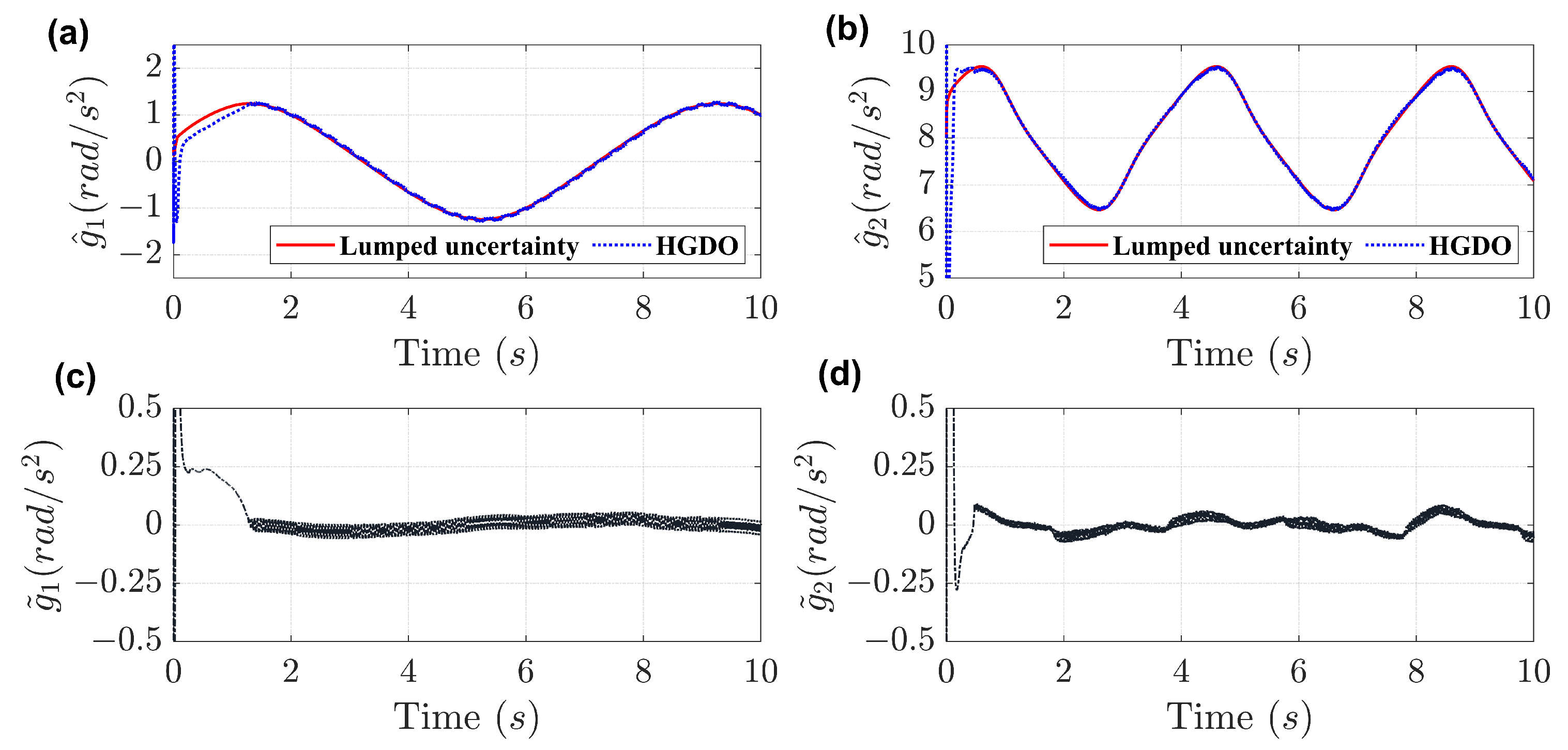
3.2. Design of the Proposed Control Framework with HGDO

In this subsection, the HGDO technique is employed to estimate the profile of lumped uncertainty, which improves the tracking precision of the state variables with respect to their references.

The lumped uncertain term $g(t,q,\dot{q})$ in (2) can be recalculated as follows:

$$\begin{array}{c}\hfill g(t,q,\dot{q})=\ddot{q}-M^{-1}\left(q\right)B\left(q\right)u-f(q,\dot{q},u)\end{array}$$

(27)

This term is estimated by $\widehat{g}$, which can be obtained as

$$\begin{array}{c}\hfill \dot{\widehat{g}}=\frac{1}{\epsilon }\left(\ddot{q}-M^{-1}\left(q\right)B\left(q\right)u-f(q,\dot{q},u)-\widehat{g}\right)\end{array}$$

(28)

where $\epsilon$ is the positive observer gain. Note that $\frac{1}{\epsilon }$ is the matrix diagonal expression and $\epsilon$ is the matrix column expression.

In order to avoid the amplified noise by the high gain, the auxiliary state variable is given by

$$\begin{array}{c}\hfill Z=\widehat{g}-\frac{\dot{q}}{\epsilon }\end{array}$$

(29)

Then, the dynamics of the auxiliary state variable are presented as follows:

$$\begin{array}{c}\hfill \dot{Z}=-\frac{1}{\epsilon }\left(Z-\frac{\dot{q}}{\epsilon }\right)+\frac{1}{\epsilon }\left(-M^{-1}\left(q\right)B\left(q\right)u-f(q,\dot{q},u)\right)\end{array}$$

(30)

Theorem 3.

For the dynamic system in (2), the HGDO technique (28) with a sufficiently large gain ensures an arbitrarily bounded estimation performance of the lumped uncertainties in finite time.

Proof. 

To prove the finite time and stability of the HGDO, let us define the estimation error $\tilde{g}=g-\widehat{g}$, then the Lyapunov function is considered as follows:

$$\begin{array}{c}\hfill V_3=\frac{1}{2}{\tilde{g}}^{\top }\tilde{g}\end{array}$$

(31)

The time derivative of $V_3$ can be rewritten as

$$\begin{array}{cc}\hfill {\dot{V}}_3& ={\tilde{g}}^{\top }\dot{\tilde{g}}\hfill \\ \hfill & ={\tilde{g}}^{\top }\left(-\frac{1}{\epsilon }\tilde{g}+\dot{g}\right)\hfill \\ \hfill & =-\frac{1}{\epsilon }{\tilde{g}}^{\top }\tilde{g}+{\tilde{g}}^{\top }\dot{g}\hfill \end{array}$$

(32)

Using Young’s inequality, ${\tilde{g}}^{\top }\dot{g}\le \frac{1}{2}{\tilde{g}}^{\top }\tilde{g}+\frac{1}{2}{\dot{g}}^{\top }\dot{g}\le \frac{1}{2}{\tilde{g}}^{\top }\tilde{g}+\frac{1}{2}{\delta }_{\dot{g}}^2$, and (4) in Assumption 1, substituting into (32) to obtain the following result:

$$\begin{array}{cc}\hfill {\dot{V}}_3& \le \left(\frac{1}{\epsilon }-\frac{1}{2}\right){\tilde{g}}^{\top }\tilde{g}+\frac{1}{2}{\delta }_{\dot{g}}^2\hfill \\ \hfill & \le -a{V}_3+b\hfill \end{array}$$

(33)

where $a=min\left(2{\Gamma }_{min}\left(\frac{1}{\epsilon }-\frac{1}{2}\right)\right)$ and $b=\frac{1}{2}{\delta }_{\dot{g}}^2$. ${\Gamma }_{min}$ represent the minimum eigenvalues of a matrix.

Multiplying ${\mathbf{e}}^{at}$ to both sides of inequality ${\dot{V}}_3$ in (33), then taking the integral with respect to time, is obtained as

$$\begin{array}{c}\hfill {\int }_{V_3\left(0\right)}^{V_3\left(t_3\right){\mathbf{e}}^{a{t}_3}}d\left(V_3{\mathbf{e}}^{at}\right)\le {\int }_0^{t_3}\frac{b}{a}{\mathbf{e}}^{at}\mathrm{d}t\end{array}$$

(34)

where $V_3\left(0\right)$ and $V_3\left(t_3\right)$ are the Lyapunov of the HGDO error at the initial position and at position $\Pi$, respectively.

Solving inequality (34), we have

$$\begin{array}{c}\hfill V_3\left(t_3\right)\le \left(V_3\left(0\right)-\frac{b}{a}\right){\mathbf{e}}^{-at}+\frac{b}{a}\end{array}$$

(35)

Due to the magnitude of $V_3\left(0\right)$ being unknown, there are two possible cases. The first case occurs when $V_3\left(0\right)\le \frac{2b}{a}$. We have $V_3\left(t_3\right)\le \frac{b}{a}{\mathbf{e}}^{-at}+\frac{b}{a}\le \frac{2b}{a}$; the error of HGDO is smaller than a constant value, $\Pi =\sqrt{\frac{4b}{a}},\forall t$, then Theorem 3 is satisfied. The second case is $V_3\left(0\right)>\frac{2b}{a}$. The magnitude of $V_3\left(t_3\right)$ is chosen as $\frac{2b}{a}$, then we obtain $\frac{b}{a}\le \left(V_3\left(0\right)-\frac{b}{a}\right){\mathbf{e}}^{-at}$. Thus, the HGDO state error will move from the initial state to $\Pi =\sqrt{\frac{4b}{a}}$ within a finite time $t_3\le \frac{1}{a}ln\left(\frac{a}{b}{V}_3\left(0\right)-1\right)$.

Hence, the proof of Theorem 3 is completed. □

Let $\tilde{g}=g-\widehat{g}$ be the estimation error. The proposed control signals (21) and (22) are redesigned based on (28) to overcome the HGDO error as

$$u_n=M\left(q\right)B^{-1}\left(q\right)\left({\ddot{q}}_d-f(q,\dot{q},u)-\widehat{g}+v^{-1}{\dot{q}}_e^{(1-v)}\Omega \right)$$

(36)

$$u_r=-M\left(q\right)B^{-1}\left(q\right){\rm Y}∥s∥∥v{\dot{q}}_e^{(v-1)}∥\left(\right||\Pi ||+\kappa )$$

(37)

where the norm of $\left|\right|\Pi \left|\right|$ is a positive constant value with the upper bounded value, i.e., $\left|\right|\Pi \left|\right|\le {\delta }_g+\tilde{g}$, which is given in detail in the proof of Theorem 3.

Theorem 4.

For the system dynamics presented in (2), with the bounded lumped uncertainty estimation satisfied in Theorem 3, the tracking error converges quickly to the equilibrium point, i.e., $q_e\cong 0$ in finite time by the designed control input (20) based on (36) and (37) while the global system stability is guaranteed.

Proof. 

To verify the finite time of the whole proposed controller, the Lyapunov function is considered as follows:

$$\begin{array}{cc}\hfill V_4& =\frac{1}{2}{s}^{\top }s\hfill \end{array}$$

(38)

Substituting (36) and (37) into (19), the time derivative of $V_4$ is computed as

$$\begin{array}{cc}\hfill {\dot{V}}_4=& s^{\top }\dot{s}\hfill \\ \hfill =& s^{\top }\left(-\Omega +v{\dot{q}}_e^{(v-1)}\left(M^{-1}\left(q\right)B\left(q\right)u+f(q,\dot{q},u)+g(t,q,\dot{q})-{\ddot{q}}_d\right)\right)\hfill \\ \hfill =& s^{\top }v{\dot{q}}_e^{(v-1)}\tilde{g}-s^{\top }v{\dot{q}}_e^{(v-1)}\frac{{\left(s^{\top }v{\dot{q}}_e^{v-1}\right)}^{\top }}{{∥s^{\top }v{\dot{q}}_e^{v-1}∥}^2}∥s∥∥v{\dot{q}}_e^{v-1}∥(∥\Pi ∥+\kappa )\hfill \\ \hfill =& s^{\top }v{\dot{q}}_e^{(v-1)}\left(\tilde{g}-\frac{{\left(s^{\top }v{\dot{q}}_e^{v-1}\right)}^{\top }}{{∥s^{\top }v{\dot{q}}_e^{v-1}∥}^2}∥s∥∥v{\dot{q}}_e^{v-1}∥(∥\Pi ∥+\kappa )\right)\hfill \\ \hfill \le & s^{\top }v{\dot{q}}_e^{(v-1)}\tilde{g}-∥v{\dot{q}}_e^{(v-1)}∥(∥\Pi ∥+\kappa )∥s∥\hfill \\ \hfill \le & ∥v{\dot{q}}_e^{(v-1)}∥\left(∥\tilde{g}∥-(∥\Pi ∥+\kappa )\right)∥s∥\hfill \end{array}$$

(39)

Based on (4) in Assumption 1, (39) can be rewritten as

$$\begin{array}{cc}\hfill {\dot{V}}_4& \le -∥v{\dot{q}}_e^{(v-1)}∥\kappa ∥s∥\hfill \\ \hfill & \le -\sigma V_4^{1/2}\hfill \end{array}$$

(40)

According to (40), the system error converges quickly to zero in finite time by the proposed control scheme, while the global system stability is guaranteed.

This completes the proof of Theorem 4. □

3.3. Design of the Proposed Control Scheme with STW

In order to eliminate the chattering phenomenon in the control system, the control law is upgraded in the reaching phase by incorporating the STW in [24]. Thus, the robust term ${\rm Y}∥s∥∥v{\dot{q}}_e^{(v-1)}∥\left(\right||\Pi ||+\kappa )$ of the control signal $u_r$ for the reaching phase in (37) can be replaced by

$$\begin{array}{c}\hfill sup\left(s\right)=k_3{\left|s\right|}^{1/2}\mathrm{sign}\left(s\right)-k_4{\int }_0^t\mathrm{sign}\left(s\right)\mathrm{d}t\end{array}$$

(41)

where the inequalities of the gain control parameters, $k_3>2\kappa$ and $k_4>k_3\frac{5k_3+4\kappa }{2k_3-4\kappa }\kappa$, are satisfied.

It is noteworthy that its stability properties are maintainedAs we know, the STW operates by dynamically adjusting the control signal to compensate for uncertainties and disturbances without requiring precise knowledge of the system dynamics. The algorithm consists of two components. First, the twisting control term reacts to the sign of the sliding variable, providing robustness and ensuring the trajectory approaches the sliding surface. The second component is the integration of the signum function which integrates the sign of the sliding variable over time, smoothing the control action and thereby reducing chattering. It is noteworthy that the sliding surface definition is crucial for control performance including the effectiveness of chattering reduction. Fortunately, the combination of the proposed SNFTSM fulfills the expectations, while the stability properties of the STW are maintained via the Lyapunov theory in [24]. The control $u_r$ is finally expressed as follows:

$$\begin{array}{c}\hfill u_r=-M\left(q\right)B^{-1}\left(q\right)sup\left(s\right)\end{array}$$

(42)

Remark 2.

According to the proven Theorems 2 and 4, the proposed manifold (5) guarantees the global finite-time convergence and stability criterion. Therefore, the newly proposed control scheme (36) presented in conjunction with the STW algorithm (42) inherits these properties. Moreover, it not only achieves rapid and smooth convergence and effective singularity avoidance but also successfully eliminates chattering in the trajectory. This comprehensive approach enhances the overall control performance and stability of the system, making it robust and accurate in diverse operating conditions.

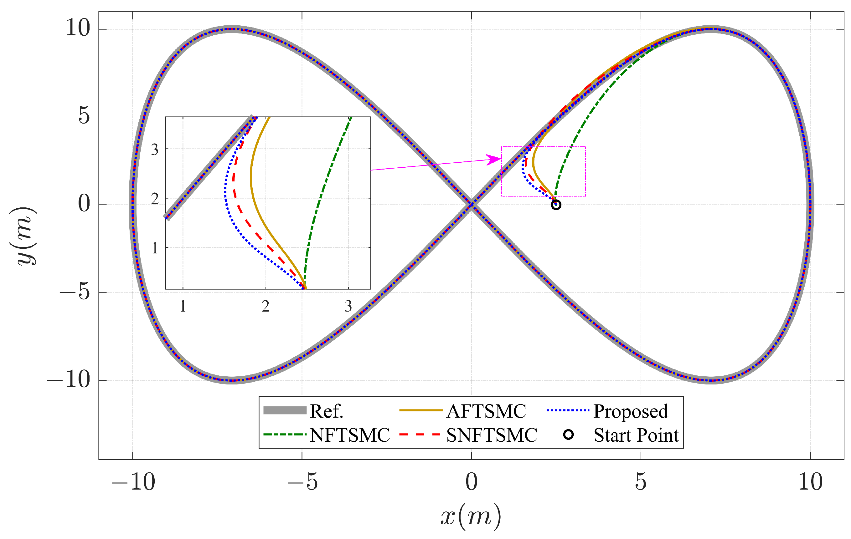
4. Numerical Examples

In this section, a numerical example is illustrated to proceed with the evaluation of the proposed control framework, the following features are assessed: response speed, accuracy, and chattering mitigation efficiency. To do that, other control methods such as the NFTSMC [33] and the AFTSMC [19] are applied in turn to demonstrate the validity of the suggested approach. Meanwhile, the SNFTSMC scheme can be regarded as a special case of the proposed control scheme, if not incorporating the HGDO estimation, for the purpose of comparison. To be fair, they are also integrated with the STW algorithm.

Remark 3.

The control signals $u_N$ and $u_A$ are generated with NFTSMC and AFTSMC as the following, respectively.

$$\begin{array}{cc}\hfill u_N=& M\left(q\right)B^{-1}\left(q\right)\left({\ddot{q}}_d-f(q,\dot{q},u)-\frac{1}{v{\kappa }_{N_1}}{\dot{q}}_e^{(2-v)}\Omega \right.\hfill \\ \hfill & -\frac{\phi {\kappa }_{N_1}}{v{\kappa }_{N_2}}{\left|q_e\right|}^{(\phi -1)}{\dot{q}}_e^{(2-v)}-k_3{\left|s\right|}^{1/2}\mathrm{sign}\left(s\right)\left.-k_4{\int }_0^t\mathrm{sign}\left(s\right)\mathrm{d}t\right)\hfill \end{array}$$

(43)

$$\begin{array}{cc}\hfill u_A=& M\left(q\right)B^{-1}\left(q\right)\left({\ddot{q}}_d-f(q,\dot{q},u)-\frac{{\kappa }_{A_1}}{1+e^{-{\eta }_{A_1}\left(\right|q_e|-\varphi )}}{\dot{q}}_e\right.\hfill \\ \hfill & -\frac{{\kappa }_{A_1}{\eta }_{A_1}{\dot{q}}_e\mathrm{sign}\left(q_e\right)e^{-{\eta }_{A_1}\left(\right|q_e|-\varphi )}}{{(1+e^{-{\eta }_{F1}\left(\right|q_e|-\varphi )})}^2}-\frac{{\kappa }_{A_2}\rho }{1+e^{-{\eta }_{A_2}\left(\right|q_e|-\varphi )}}{\left|q_e\right|}^{(\rho -1)}{\dot{q}}_e\hfill \\ \hfill & -\frac{{\kappa }_{A_2}{\eta }_{A_2}{\dot{q}}_e{e}^{-{\eta }_{A_2}\left(\right|q_e|-\varphi )}}{{(1+e^{-{\eta }_{A_1}\left(\right|q_e|-\varphi )})}^2}{\left|q_e\right|}^{\rho }-k_3{\left|s\right|}^{1/2}\mathrm{sign}\left(s\right)\left.-k_4{\int }_0^t\mathrm{sign}\left(s\right)\mathrm{d}t\right)\hfill \end{array}$$

(44)

The parameters of those control algorithms are chosen as: $v=\varphi =5/3$, $\rho =1/v=3/5$, ${\kappa }_{A_1}={\kappa }_{N_1}=k_1=\mathrm{diag}\left([0.5,0.5]\right)$, ${\kappa }_{A_2}={\kappa }_{N_2}=k_2=\mathrm{diag}\left([1,1]\right)$, $k_3=\mathrm{diag}\left([10,10]\right)$, $k_4=\mathrm{diag}\left([3,3]\right)$, ${\eta }_1=0.1$, ${\eta }_2=0.1$, $\alpha =2$, $\beta =2$, $\gamma =1$, $m_v=5$, $n_v=3$, $ϵ=0.002$. The formulations of system matrices $M,V,B,\mathrm{\Lambda }$ are derived in Appendix A, in which $m=1.8$ kg, $I=0.0028$ kg · m² and $I_w=0.008$ kg · m² are the mass, the total equivalent inertia, and the inertia for each driving wheel of the AGV, respectively; each driving wheel has the radius of $R=0.033$ m with a motor about the wheel axis; $L=0.1435$ m is the distance between two wheels; the objective is to track a lemniscate trajectory described by $q_d\left(t\right)={\left[\begin{array}{ccc}{x}_d\left(t\right)& y_d\left(t\right)& \mathrm{atan}2\left({\dot{x}}_d\left(t\right),{\dot{y}}_d\left(t\right)\right)\end{array}\right]}^{\top }$, with $x_d\left(t\right)=10sin\left(\frac{\pi }{2}t\right)$; $y_d\left(t\right)=10sin\left(\frac{\pi }{4}t\right)$; where $\mathrm{atan}2(·,·)$ is the four-quadrant inverse tangent function; $T_d=m·g·sin\left({\theta }_d\right)·R$ with moving on an incline of ${\theta }_d=5^{\circ }$; $f_c=b·\dot{q}+{\mu }_s·m·g$ with the viscous damping coefficient $b=0.5$ and the coefficient of static friction ${\mu }_s=1$ between the AGV’s wheels and the surface; $d={10}^{-3}$ m; $g=9.81$ m/s². To establish the transformation of coordinates between the two coordinate systems in Figure 2, it is the world coordinate system denoted as $XOY$ and the vehicle coordinate system denoted as $xoy$, in which $\theta$ represents the rotation angle between those coordinates and ($x_c$, $y_c$) is the coordinates of the origin $\mathit{o}$ in the $XOY$ system. Utilizing the homogeneous coordinate form, the transformations of coordinates between the two coordinate systems can be expressed as follows:

$$\begin{array}{c}\hfill \left[\begin{array}{c}x\\ y\\ 1\end{array}\right]=\left[\begin{array}{ccc}cos\theta & sin\theta & 0\\ -sin\theta & cos\theta & 0\\ 0& 0& 1\end{array}\right]\left[\begin{array}{ccc}1& 0& -x_c\\ 0& 1& -y_c\\ 0& 0& 1\end{array}\right]\left[\begin{array}{c}X\\ Y\\ 1\end{array}\right]\end{array}$$

(45)

or,

$$\begin{array}{c}\hfill \left[\begin{array}{c}X\\ Y\\ 1\end{array}\right]=\left[\begin{array}{ccc}1& 0& x_c\\ 0& 1& y_c\\ 0& 0& 1\end{array}\right]\left[\begin{array}{ccc}cos\theta & -sin\theta & 0\\ sin\theta & cos\theta & 0\\ 0& 0& 1\end{array}\right]\left[\begin{array}{c}x\\ y\\ 1\end{array}\right]\end{array}$$

(46)

In the tracking trajectory scenario, Figure 3 displays the trajectories of the coordinates of the origin $\mathit{o}(x_c,y_c)$ with the start point ${[2.5,0,\pi /2]}^{\top }$, where the gray line is the desired trajectory and the other lines are the performance responses. Specifically, the green dashed–dotted line, brown line, red dashed line, and blue dotted line denote the results by applying the NFTSMC, the AFTSMC, the SNFTSMC, and the proposed control scheme, respectively.

It can be observed from Figure 3 that all controllers achieve the desired tracking performance. However, the sliding surface by the proposed approach significantly improves the efficiency of the output response. To be more specific, the tracking errors of the system state and the cross-track error (XTE) under uncertainty/disturbance conditions are presented in Figure 4, in which the XTE is defined as the minimum distance of the current position to the reference trajectory. Here, the proposed controller achieves the best convergence rate at around $0.4$ s with the assistance of both the proposed surface and the HGDO technique. Although the convergence rate of the proposed controller is only slightly faster in comparison with the AFTSMC, the AFTSMC carries the risk of encountering singularity issues during the operation process. Thus, the controllers using the proposed sliding surface with the nonsingular property can be potential candidates for fast finite-time tracking control. Owing to the merits of the STW algorithm, steady-state tracking performance by the four controllers is nearly identical with very small errors within negligible chattering. In addition, Figure 5 displays the control input signals corresponding to the four control strategies. These results reveal a slight initial overshoot due to the rapid convergence rate. However, the control methods incorporating the STW algorithm substantially eliminate the chattering phenomenon in the output trajectory. In brief, the proposed controller outperforms the other strategies, exhibiting the smallest steady-state tracking error. This outcome confirms the finite-time convergence characteristic of the closed-loop system and ensures guaranteed global stability, solidifying the superior performance of the proposed control scheme. Furthermore, the estimation performance of the HGDO is also investigated and the results indicate a good estimation performance with small errors in a range of $\pm 0.1$ rad/s², as shown in Figure 6. It implies that the estimated values are closely fitted with the actual uncertainty value, i.e., the lumped uncertainty is successfully estimated by the HGDO approach. Accordingly, the HGDO technique provides great estimation results for uncertainties. In order to quantitatively compare the effectiveness of these control approaches, we consider two performance indices, the integral of the absolute square value of tracking error (IASE) and control efforts (IASC) [30]. The results in Figure 7 reaffirm that the effectiveness of the proposed control framework achieves the smallest error values with the least effort. The proposed control scheme integrated with the STW and HGDO techniques enables an effective controller design against uncertainties and disturbances.

5. Conclusions

In this study, the proposed SNFTSM-based control scheme that integrates the STW algorithm and the HGDO technique was applied to the AGV system to exhibit its outstanding features. According to the obtained results and comparisons, the main contributions of this paper are as follows: (1) converges to the equilibrium point of the sliding phase in finite time, (2) mitigates chattering phenomenon in the trajectory, (3) successfully estimates the uncertainties and external disturbances, and (4) eliminates the singularity in the sliding manifold. Moreover, the system stability with the designed controller is guaranteed by the Lyapunov theory, which is validated through numerical simulations. Since the proposed approach has been described with generality, many modifiable variables may seem complicated to follow. However, in fact, the sliding surface design could be simplified for specific systems.

References

1. Taheri, H.; Zhao, C.X. Omnidirectional mobile robots, mechanisms and navigation approaches. Mech. Mach. Theory 2020, 153, 103958. [Google Scholar] [CrossRef]
2. Peng, H.; Li, F.; Liu, J.; Ju, Z. A Symplectic Instantaneous Optimal Control for Robot Trajectory Tracking With Differential-Algebraic Equation Models. IEEE Trans. Ind. Electron. 2020, 67, 3819–3829. [Google Scholar] [CrossRef]
3. Li, S.; Ding, L.; Gao, H.; Chen, C.; Liu, Z.; Deng, Z. Adaptive neural network tracking control-based reinforcement learning for wheeled mobile robots with skidding and slipping. Neurocomputing 2018, 283, 20–30. [Google Scholar] [CrossRef]
4. Tang, Y. Terminal sliding mode control for rigid robots. Automatica 1998, 34, 51–56. [Google Scholar] [CrossRef]
5. Choi, J.; Lee, G.; Lee, C. Reinforcement learning-based dynamic obstacle avoidance and integration of path planning. Intell. Serv. Robot. 2021, 14, 663–677. [Google Scholar] [CrossRef]
6. Vo, C.P.; Lee, J.; Jeon, J.H. Robust Adaptive Path Tracking Control Scheme for Safe Autonomous Driving via Predicted Interval Algorithm. IEEE Access 2022, 10, 124333–124344. [Google Scholar] [CrossRef]
7. Liu, Y.; Wang, Y.; Guan, X.; Hu, T.; Zhang, Z.; Jin, S.; Wang, Y.; Hao, J.; Li, G. Direction and Trajectory Tracking Control for Nonholonomic Spherical Robot by Combining Sliding Mode Controller and Model Prediction Controller. IEEE Robot. Autom. Lett. 2022, 7, 11617–11624. [Google Scholar] [CrossRef]
8. Vo, C.P.; Jeon, J.H. An Integrated Motion Planning Scheme for Safe Autonomous Vehicles in Highly Dynamic Environments. Electronics 2023, 12, 1566. [Google Scholar] [CrossRef]
9. Chen, X.; Zhao, H.; Sun, H.; Zhen, S.; Huang, K. A novel adaptive robust control approach for underactuated mobile robot. J. Frank. Inst. 2019, 356, 2474–2490. [Google Scholar] [CrossRef]
10. Xie, Y.; Zhang, X.; Meng, W.; Zheng, S.; Jiang, L.; Meng, J.; Wang, S. Coupled fractional-order sliding mode control and obstacle avoidance of a four-wheeled steerable mobile robot. ISA Trans. 2021, 108, 282–294. [Google Scholar] [CrossRef] [PubMed]
11. Feng, X.; Wang, C. Robust Adaptive Terminal Sliding Mode Control of an Omnidirectional Mobile Robot for Aircraft Skin Inspection. Int. J. Control Autom. Syst. 2021, 19, 1078–1088. [Google Scholar] [CrossRef]
12. Taghavifar, H.; Mohammadzadeh, A. Adaptive Robust Terminal Sliding Mode Control with Integral Backstepping Synthesized Method for Autonomous Ground Vehicle Control. Vehicles 2023, 5, 1013–1029. [Google Scholar] [CrossRef]
13. Nguyen, N.P.; Oh, H.; Moon, J. Continuous Nonsingular Terminal Sliding-Mode Control With Integral-Type Sliding Surface for Disturbed Systems: Application to Attitude Control for Quadrotor UAVs Under External Disturbances. IEEE Trans. Aerosp. Electron. Syst. 2022, 58, 5635–5660. [Google Scholar] [CrossRef]
14. Han, Y.; Cheng, Y.; Xu, G. Trajectory Tracking Control of AGV Based on Sliding Mode Control With the Improved Reaching Law. IEEE Access 2019, 7, 20748–20755. [Google Scholar] [CrossRef]
15. Jiang, B.; Li, J.; Yang, S. An improved sliding mode approach for trajectory following control of nonholonomic mobile AGV. Sci. Rep. 2022, 12, 17763. [Google Scholar] [CrossRef] [PubMed]
16. Vo, C.P.; Ahn, K.K. An Adaptive Finite-Time Force-Sensorless Tracking Control Scheme for Pneumatic Muscle Actuators by an Optimal Force Estimation. IEEE Robot. Autom. Lett. 2022, 7, 1542–1549. [Google Scholar] [CrossRef]
17. Wu, Y.; Wang, L.; Zhang, J.; Li, F. Path Following Control of Autonomous Ground Vehicle Based on Nonsingular Terminal Sliding Mode and Active Disturbance Rejection Control. IEEE Trans. Veh. Technol. 2019, 68, 6379–6390. [Google Scholar] [CrossRef]
18. Hajjami, L.E.; Mellouli, E.M.; Berrada, M. Robust adaptive non-singular fast terminal sliding-mode lateral control for an uncertain ego vehicle at the lane-change maneuver subjected to abrupt change. Int. J. Dyn. Control 2021, 9, 1765–1782. [Google Scholar] [CrossRef]
19. Vo, A.T.; Kang, H.J. A Novel Fault-Tolerant Control Method for Robot Manipulators Based on Non-Singular Fast Terminal Sliding Mode Control and Disturbance Observer. IEEE Access 2020, 8, 109388–109400. [Google Scholar] [CrossRef]
20. Du, S.; Liu, Y.; Wang, Y.; Li, Y.; Yan, Z. Research on a Permanent Magnet Synchronous Motor Sensorless Anti-Disturbance Control Strategy Based on an Improved Sliding Mode Observer. Electronics 2023, 12, 4188. [Google Scholar] [CrossRef]
21. Luo, M.; Yu, Z.; Xiao, Y.; Xiong, L.; Xu, Q.; Ma, L.; Wu, Z. Full-order adaptive sliding mode control with extended state observer for high-speed PMSM speed regulation. Sci. Rep. 2023, 13, 6200. [Google Scholar] [CrossRef] [PubMed]
22. Edelbaher, G.; Jezernik, K.; Urlep, E. Low-speed sensorless control of induction Machine. IEEE Trans. Ind. Electron. 2006, 53, 120–129. [Google Scholar] [CrossRef]
23. Wang, L.; Chen, C.L.P. Reduced-Order Observer-Based Dynamic Event-Triggered Adaptive NN Control for Stochastic Nonlinear Systems Subject to Unknown Input Saturation. IEEE Trans. Neural Netw. Learn. Syst. 2021, 32, 1678–1690. [Google Scholar] [CrossRef] [PubMed]
24. Moreno, J.A.; Osorio, M. A Lyapunov approach to second-order sliding mode controllers and observers. In Proceedings of the 2008 47th IEEE Conference on Decision and Control, Cancun, Mexico, 9–11 December 2008; pp. 2856–2861. [Google Scholar]
25. Chalanga, A.; Kamal, S.; Fridman, L.M.; Bandyopadhyay, B.; Moreno, J.A. Implementation of Super-Twisting Control: Super-Twisting and Higher Order Sliding-Mode Observer-Based Approaches. IEEE Trans. Ind. Electron. 2016, 63, 3677–3685. [Google Scholar] [CrossRef]
26. Al-Mayyahi, A.; Wang, W.; Birch, P. Adaptive Neuro-Fuzzy Technique for Autonomous Ground Vehicle Navigation. Robotics 2014, 3, 349–370. [Google Scholar] [CrossRef]
27. Huang, D.; Zhai, J.; Ai, W.; Fei, S. Disturbance observer-based robust control for trajectory tracking of wheeled mobile robots. Neurocomputing 2016, 198, 74–79. [Google Scholar] [CrossRef]
28. Li, L.; Wang, T.; Xia, Y.; Zhou, N. Trajectory tracking control for wheeled mobile robots based on nonlinear disturbance observer with extended Kalman filter. J. Frank. Inst. 2020, 357, 8491–8507. [Google Scholar] [CrossRef]
29. Neĭmark, I.I.; Fufaev, N.A.; Barbour, J.R. Dynamics of Nonholonomic Systems. In Translations of Mathematical Monographs; American Mathematical Society: Providence, RI, USA, 1972. [Google Scholar]
30. Vo, C.P.; To, X.D.; Ahn, K.K. A Novel Adaptive Gain Integral Terminal Sliding Mode Control Scheme of a Pneumatic Artificial Muscle System With Time-Delay Estimation. IEEE Access 2019, 7, 141133–141143. [Google Scholar] [CrossRef]
31. Feng, Y.; Yu, X.; Man, Z. Non-singular terminal sliding mode control of rigid manipulators. Automatica 2002, 38, 2159–2167. [Google Scholar] [CrossRef]
32. Bloch, A.M.; Crouch, P.; Baillieul, J.; Marsden, J. Nonholonomic Mechanics and Control. Appl. Mech. Rev. 2004, 57. [Google Scholar] [CrossRef]
33. Li, S.; He, Z.; Liu, C.; Zhan, Y.; Li, H.; Huang, X.; Zhang, Z. Nonsingular Fast Terminal Sliding Mode Control with Extended State Observer and Tracking Differentiator for Uncertain Nonlinear Systems. Math. Probl. Eng. 2014, 2014, 639707. [Google Scholar]
Figure 1. Structure of the closed-loop AGV system under the proposed control scheme with STW and HGDO.
Mathematics 12 00549 g001
Figure 2. The coordinate system of the AGV.
Mathematics 12 00549 g002
Figure 3. The path-following performance for a desired infinity-shaped trajectory by different approaches.
Mathematics 12 00549 g003
Figure 4. Tracking performance of all controllers; (a) the x coordinates and (b) the y coordinates of the origin; (c) the cross-tracking errors.
Mathematics 12 00549 g004
Figure 5. System-controlled input signals for all algorithms; (a) left and (b) right actuators.
Mathematics 12 00549 g005
Figure 6. Estimation performance of HGDO technique; (a,b) The lumped value and the estimated value of uncertainty and disturbance terms in left and right actuators, respectively; (c,d) Its estimation errors.
Mathematics 12 00549 g006
Figure 7. Performance indices involving the integral of absolute squares (IAS); (a) tracking error; (b) the control input.
Mathematics 12 00549 g007
Disclaimer/Publisher’s Note: The statements, opinions and data contained in all publications are solely those of the individual author(s) and contributor(s) and not of MDPI and/or the editor(s). MDPI and/or the editor(s) disclaim responsibility for any injury to people or property resulting from any ideas, methods, instructions or products referred to in the content.