Abstract
We consider the inverse scattering problem to reconstruct an obstacle using partial far-field data due to one incident wave. A simple indicator function, which is negative inside the obstacle and positive outside of it, is constructed and then learned using a deep neural network (DNN). The method is easy to implement and effective as demonstrated by numerical examples. Rather than developing sophisticated network structures for the classical inverse operators, we reformulate the inverse problem as a suitable operator such that standard DNNs can learn it well. The idea of the DNN-oriented indicator method can be generalized to treat other partial data inverse problems.
MSC:
65N21; 78A46
1. Introduction
Inverse scattering problems arise in many areas such as medical imaging and seismic detection. The scattering from obstacles leads to exterior boundary value problems for the Helmholtz equation. The two-dimensional case is derived from the scattering from finitely long cylinders, and more importantly, it can serve as a model case for testing numerical approximation schemes in direct and inverse scattering [1]. In this paper, we consider the inverse problem to reconstruct an obstacle, given partial far-field data in .
Let be a bounded domain with a -boundary . Denoting by the incident plane wave, the direct scattering problem for a sound-soft obstacle is to find the scattered field such that
where is the wavenumber. It is well known that has an asymptotic expansion
uniformly in all directions . The function defined on is the far-field pattern of for D due to the incident field . The inverse problem of interest is to reconstruct D from n far-field patterns for one incident wave. Note that the unique determination of D using the far-field pattern due to one incident wave is an open problem.
Classical inverse scattering methods to reconstruct an obstacle mainly fall into two groups. The first group is the optimization methods to minimize certain cost functions [2,3]. These methods usually solve a number of direct scattering problems and work well when proper initial guesses are available. The second group is the sampling methods, e.g., the linear sampling method, the extended sampling method, the orthogonality method, the reverse time migration, and the direct sampling method [4,5,6,7,8]. These methods often construct some indicator functions based on the analysis of the partial differential equations to determine if a sampling point is inside or outside the obstacle. In contrast to the optimization methods, the sampling methods do not need initial guesses and forward solvers but usually provide less information of the unknown obstacle.
Although successful for many cases, classical methods have difficulties for problems with partial data. For example, the linear sampling method cannot obtain a reasonable reconstruction if the data are collected on a small aperture. Recently, there has been an increasing interest in solving inverse problems using deep neural networks (DNNs). Various DNNs have been proposed to reconstruct the obstacle from the scattered field [9,10,11,12]. Although the deep learning methods can process partial data, the performance is highly problem-dependent and the network structures are often sophisticated. Combinations of deep learning and sampling methods for the inverse scattering problems have also been investigated recently [13,14,15,16]. These methods usually construct a DNN to learn the reconstruction of some sampling method.
In this paper, we propose a DNN-oriented indicator method. The idea is to design an indicator function which is simple enough for standard DNNs to learn it effectively. We borrow from the sampling methods the concept of the indicator. What sets our method apart from the sampling methods is that the indicator is defined as a signed distance function other than using the inner product related to Green’s function or solving the linear ill-posed integral equations. The indicator is then learned by a DNN with partial scattering data as input. This DNN-oriented indicator method inherits the advantage of deep learning methods by compensating for partial information through empirical data. Meanwhile, it retains the simplicity and flexibility of sampling methods. Numerical experiments demonstrate its effectiveness for obstacle reconstructions with a few far-field data due to one incident wave. Note that the idea is to find a formulation for the inverse problem that is easy to learn instead of the design of sophisticated neural networks (see [17]).
2. Dnn-Oriented Indicator Method
We propose a DNN-oriented indicator method for the inverse obstacle scattering problem in . The framework can be directly applied to other inverse problems and extended to . For an obstacle D, we define a signed distance function
It is clear that is a continuous function with respect to and can be used to reconstruct the obstacle since
Let be the vector of far-field data due to one incident wave in n observation directions. Let be a (large) domain, known as a prior, containing D. For a point , we define the indicator function as
Our goal is to design a DNN to learn for input . More specifically, we expect to build a neural network to approximate the indicator function I. The input of is a vector in consisting of the real and imaginary parts of and the coordinates of a point . The output is the corresponding signed distance. Assume that there are L hidden layers for . Each hidden layer is defined as
where and are the input and output vectors of the lth layer, respectively, is the output weight matrix, and is the bias vector. The non-linear function is the rectified linear unit (ReLU) defined as . The input layer with output weight matrix and bias vector is connected to the first hidden layer.
A set of N data is used to train the fully connected network . The set of parameters is denoted by and is updated by the backpropagation algorithm, minimizing the half quadratic error of the predicted responses between the set of training mapped measurements and exact values . The loss function is the half mean-squared error given by
The algorithm for the DNN-oriented indicator method is illustrated in Algorithm 1. It contains an offline phase and an online phase. In the offline phase, the training data are used to learn the network parameters. Then, the network is used in the online phase to output the indicator for each . Using the same notation for the function produced by the trained network , indicates that , whereas indicates that . The approximate support of D can be reconstructed accordingly.
| Algorithm 1 DNN-oriented indicator method. |
offline phase
online phase
|
Remark 1.
Other indicator functions, e.g., the characteristic function for D, can be used and have similar performance. The advantage of the indicator function (3) is that it provides information on the distance of a point to the boundary of the obstacle.
Remark 2.
The set Ω in the offline phase and online phase can be different, which allows additional flexibility.
3. Numerical Experiments
We present some numerical examples to demonstrate the proposed DNN-oriented indicator method. All the experiments are conducted on a laptop with an Intel(R) Core(TM) i7-10510U CPU @ 1.80 GHz (up to 2.30 GHz) and 16 GB of RAM.
The wave number is , and the incident plane wave is with . The training data are generated using a boundary integral method for (1) [1]. The observation data contain the far-field patterns of 6 observation directions
uniformly distributed on one-quarter of the unit circle.
For the offline phase, we use random obstacles which are star-shaped domains [18]:
where
In the experiments, and the coefficients , , are uniformly distributed random numbers. We use points uniformly distributed in the region . The training data consist of for each obstacle and each sampling point as input and the signed distance function at for as output. The size of the training set is .
The neural network is fully connected feed-forward with layers and the numbers of nodes in each layer are , respectively, where the number of hidden layers L and the number of neurons in each hidden layer are chosen using the rule of thumb [19] and a trial-and-error method. The network is trained for up to iterations using a mini-batch size of 300 and 4 epochs. We normalize the input per feature to zero mean and standard deviation one, and use the adaptive moment estimation (Adam) with an initial learning rate of , gradually reducing the learning rate by a factor of every 3 epochs. When and , the training duration is approximately 13 min and 57 s, while the testing duration is less than 1 s.
To evaluate the effectiveness of the DNN , we generate a test set of size . The following relative error for the test set is used:
We test the network with different L and and show the relative errors utilizing noiseless far-field data and far-field data with random noises in Table 1. For each L, the upper row is for the noiseless data and the lower row is for noisy data. Since the errors are smaller for and , we use them for in the online phase.

Table 1.
Relative errors for DNNs with different L and .
Remark 3.
The results indicate that the inverse operator only needs a simple network with reasonably small L and . More sophisticated networks negatively affect the performance.
Remark 4.
The complexity of the neural network depends on various elements, including the number and locations of far-field data, the wavenumber k, etc. One would expect different and L for different settings.
To visualize the reconstructions, we use three obstacles: a triangle with boundary given by
a peanut with boundary given by
a kite with boundary given by
and a square whose vertices are
Let the uniformly distributed point set T for be
For each , the trained DNN is used to predict . We plot the contours for with respect to , and obtain the reconstructions by finding all such that .
For the triangle obstacle, Figure 1 shows the contour plot of the indicator function using 6 far-field data with random noise, and the reconstruction of D formed by points satisfying . Similar results for the peanut, kite and square are shown in Figure 2, Figure 3 and Figure 4, respectively. The location and size of the obstacle can be reconstructed well, taking the amount of data used into account.
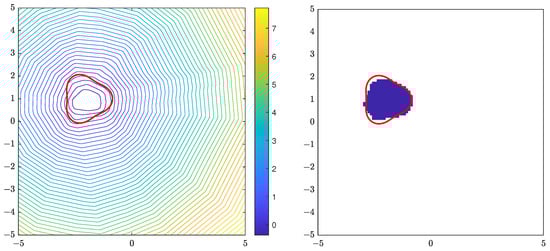
Figure 1.
The true triangle is the red line. (Left): contour plot of . (Right): reconstruction D.
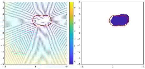
Figure 2.
The true peanut is the red line. (Left): contour plot of . (Right): reconstruction D.
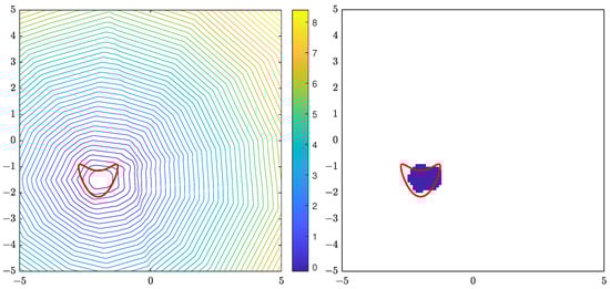
Figure 3.
The true kite is the red line. (Left): contour plot of . (Right): reconstruction D.
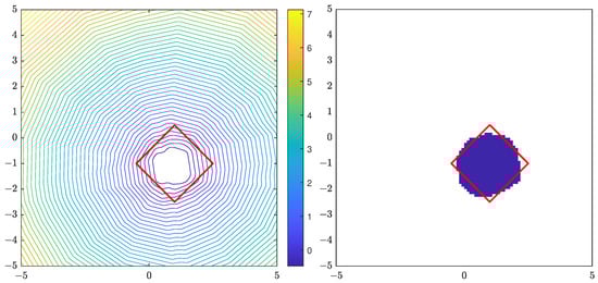
Figure 4.
The true square is the red line. (Left): contour plot of . (Right): reconstruction D.
4. Conclusions
We consider the reconstruction of a sound-soft obstacle using only a few far-field data due to a single incident wave. In addition to the inherent nonlinearity and ill-posedness of inverse problems, the presence of partial data introduces additional challenges for classical methods. In this paper, we propose a simple and novel DNN-oriented indicator method for this inverse problem, utilizing an indicator function to determine whether any chosen sample point is inside the scatterer, thus identifying the scatterer. What distinguishes this method from existing sampling methods is that our indicator function no longer relies on solving integrals or integral equations. Instead, it is defined as a signed distance function approximated using standard deep neural networks.
Rather than developing sophisticated networks, we focus on the formulation of suitable inverse operators and data structures such that standard DNNs can be employed. This method maintains the simplicity and flexibility of using indicators in reconstructing scatterers. In comparison to the existing sampling methods, it leverages the advantages of deep learning methods by compensating for insufficient known information through empirical data, allowing it to work effectively even with limited far-field data. Numerical experiments demonstrate that the location and size of the obstacle are reconstructed effectively. Such a reconstruction can serve as a starting point for other methods.
Since the performance of a DNN is highly dependent on the training data, data tailored for single scatterers in the numerical implementation can only train a deep neural network suitable for the reconstruction of single scatterers. In the future, we plan to introduce training data for multiple scatterers and extend the idea of the DNN-oriented indicator method to other inverse problems involving partial data.
Author Contributions
Methodology, J.L. and J.S.; software, Y.L. and X.Y.; data curation, Y.L. and X.Y.; writing—original draft preparation, Y.L. and X.Y.; writing—review and editing, J.L. and J.S.; project administration, J.S.; funding acquisition, J.L. All authors have read and agreed to the published version of the manuscript.
Funding
This research was funded by NSFC grant number 11801218.
Data Availability Statement
Data sharing is not applicable.
Conflicts of Interest
The authors declare no conflicts of interest.
References
- Colton, D.L.; Kress, R.; Kress, R. Inverse Acoustic and Electromagnetic Scattering Theory; Springer: London, UK, 2019; Volume 93. [Google Scholar]
- Hettlich, F. Fréchet derivatives in inverse obstacle scattering. Inverse Probl. 1995, 11, 371. [Google Scholar] [CrossRef]
- Johansson, T.; Sleeman, B.D. Reconstruction of an acoustically sound-soft obstacle from one incident field and the far-field pattern. IMA J. Appl. Math. 2007, 72, 96–112. [Google Scholar] [CrossRef]
- Colton, D.; Haddar, H. An application of the reciprocity gap functional to inverse scattering theory. Inverse Probl. 2005, 21, 383. [Google Scholar] [CrossRef]
- Potthast, R. A study on orthogonality sampling. Inverse Probl. 2010, 26, 074015. [Google Scholar] [CrossRef]
- Ito, K.; Jin, B.; Zou, J. A direct sampling method to an inverse medium scattering problem. Inverse Probl. 2012, 28, 025003. [Google Scholar] [CrossRef]
- Chen, J.; Chen, Z.; Huang, G. Reverse time migration for extended obstacles: Acoustic waves. Inverse Probl. 2013, 29, 085005. [Google Scholar] [CrossRef]
- Liu, J.; Sun, J. Extended sampling method in inverse scattering. Inverse Probl. 2018, 34, 085007. [Google Scholar] [CrossRef]
- Chen, X.; Wei, Z.; Maokun, L.; Rocca, P. A review of deep learning approaches for inverse scattering problems (invited review). Prog. Electromagn. Res. 2020, 167, 67–81. [Google Scholar] [CrossRef]
- Gao, Y.; Zhang, K. Machine learning based data retrieval for inverse scattering problems with incomplete data. J. Inverse -Ill-Posed Probl. 2021, 29, 249–266. [Google Scholar] [CrossRef]
- Sun, Y.; He, L.; Chen, B. Application of neural networks to inverse elastic scattering problems with near-field measurements. Electron. Res. Arch. 2023, 31, 7000–7020. [Google Scholar] [CrossRef]
- Yang, H.; Liu, J. A qualitative deep learning method for inverse scattering problems. Appl. Comput. Electromagn. Soc. J. (ACES) 2020, 35, 153–160. [Google Scholar]
- Guo, R.; Jiang, J. Construct deep neural networks based on direct sampling methods for solving electrical impedance tomography. SIAM J. Sci. Comput. 2021, 43, B678–B711. [Google Scholar] [CrossRef]
- Le, T.; Nguyen, D.L.; Nguyen, V.; Truong, T. Sampling type method combined with deep learning for inverse scattering with one incident wave. arXiv 2022, arXiv:2207.10011. [Google Scholar]
- Ning, J.; Han, F.; Zou, J. A direct sampling-based deep learning approach for inverse medium scattering problems. arXiv 2023, arXiv:2305.00250. [Google Scholar] [CrossRef]
- Ruiz, Á.Y.; Cavagnaro, M.; Crocco, L. A physics-assisted deep learning microwave imaging framework for real-time shape reconstruction of unknown targets. IEEE Trans. Antennas Propag. 2022, 70, 6184–6194. [Google Scholar] [CrossRef]
- Du, H.; Li, Z.; Liu, J.; Liu, Y.; Sun, J. Divide-and-conquer DNN approach for the inverse point source problem using a few single frequency measurements. Inverse Probl. 2023, 39, 115006. [Google Scholar] [CrossRef]
- Gao, Y.; Liu, H.; Wang, X.; Zhang, K. On an artificial neural network for inverse scattering problems. J. Comput. Phys. 2022, 448, 110771. [Google Scholar] [CrossRef]
- Heaton, J. Introduction to Neural Networks with Java; Heaton Research, Inc.: Chesterfield, MO, USA, 2008. [Google Scholar]
Disclaimer/Publisher’s Note: The statements, opinions and data contained in all publications are solely those of the individual author(s) and contributor(s) and not of MDPI and/or the editor(s). MDPI and/or the editor(s) disclaim responsibility for any injury to people or property resulting from any ideas, methods, instructions or products referred to in the content. |
© 2024 by the authors. Licensee MDPI, Basel, Switzerland. This article is an open access article distributed under the terms and conditions of the Creative Commons Attribution (CC BY) license (https://creativecommons.org/licenses/by/4.0/).