Article

A Study on Determining the Optimal Feedback Rate in Distributed Block Diagonalization with Limited Feedback for Dense Cellular Networks

School of Electronic and Electrical Engineering, Kyungpook National University, Daegu 41566, Republic of Korea
*
Author to whom correspondence should be addressed.
Mathematics 2024, 12(3), 460; https://doi.org/10.3390/math12030460
Submission received: 24 December 2023 / Revised: 28 January 2024 / Accepted: 29 January 2024 / Published: 31 January 2024

Abstract

:
In this study, we explore a downlink cellular network where each base station (BS) engages in simultaneous communication with multiple users through spatial division multiple access (SDMA). The positions of both BSs and users are established through independent random point processes, effectively representing the cellular network. SDMA utilizes block diagonalization (BD) at each BS, employing multiple receive antennas for each user. To implement BD, users quantize and provide feedback on their downlink channels to their respective BSs. The net spectral efficiency, measuring the effective rate accounting for both downlink and uplink resource usage, serves as a performance metric. In prior research, the optimal feedback rate in terms of maximizing net spectral efficiency has been approximated in this scenario. The corresponding approximations effectively illustrate the asymptotic behavior of the optimal number as a function of the length of the coherent channel block. However, the accuracy of the approximation diminishes when the length of the coherent channel block is relatively small. Given that the length of the coherent channel block can assume relatively small values depending on wireless environments, achieving a precise estimate across the entire range of the coherent block length holds significant importance. Consequently, this paper focuses primarily on enhancing the accuracy of the approximation for the optimal feedback rate. In order to achieve a more precise estimation, we analyze the derivative of the net spectral efficiency, which encompasses two functions that demonstrate distinct growth rates. In contrast to prior studies, both functions are rigorously approximated through mathematical analysis. As a result, the proposed approximation significantly improves the accuracy compared to previous studies, particularly when dealing with short coherent channel block lengths. Moreover, this approximation generally achieves near-optimal performance, regardless of system parameters.

1. Introduction

In the downlink of multi-user multiple-input and multiple-output (MU-MIMO) systems, the amount of channel-state information (CSI) available at the transmitter (CSIT) holds significant importance. Because individual users lack the capability to access the received signals of other users, joint signal processing among the received signals of different users is not feasible. As a result, the transmitter generally engages in appropriate signal processing to multiplex independent signals prepared for different users. Therefore, the accuracy of CSIT remains crucial and typically determines the achievable rate within the system [1]. Securing precise CSIT presents difficulties in real-world systems, especially in frequency division duplex (FDD) systems. In FDD systems, tracking the downlink channel directly at the transmitter becomes challenging due to the separation of uplink and downlink transmission in the frequency domain. Consequently, it is a common practice in FDD-based systems to collect CSI feedback from users, establishing partial or limited CSIT. This approach, referred to as limited feedback, requires each user to estimate its own CSI through pilots, quantize the obtained information, and then provide feedback to the transmitter [2].
To evaluate the effectiveness of MU-MIMO systems based on limited feedback in realistic situations, recent research has employed probabilistic models to simulate cellular networks. These models utilize stochastic geometry to depict the locations of both base stations (BSs) and users. This method allows for the calculation of average performance metrics in communication systems across the random point process. Consequently, it streamlines the mathematical analysis regardless of the number of BSs in the network. For example, research such as [3,4,5] employed a stochastic geometry to model the positions of BSs. It was utilized to theoretically analyze the essential performance metrics in cellular networks, including the capacity and outage probability of MIMO systems, assuming a perfect CSI for both transmitters and receivers. In a different context, the authors in [6] utilized a homogeneous α -Ginibre point process to introduce a cyber insurance framework that focuses on the physical layer security of wireless communication. In the works of [7,8], stochastic geometry played a fundamental role in modeling mmWave communication for heterogeneous networks. Furthermore, numerous investigations have delved into the downlink rate in cellular networks achieved by MU-MIMO systems with limited feedback. These studies leveraged stochastic geometry to simulate realistic cellular environments, as evidenced by [9,10,11,12]. The study in [9] focused on estimating the optimal feedback rate that maximizes the net spectral efficiency. This analysis assumed the use of zero-forcing beamforming with limited feedback at each BS. The authors in [10] extended the investigation to provide both approximate lower and upper bounds for the optimal feedback rate. They also delved into the exploration of associated estimation errors. In [11], the focus is on identifying the optimal number of bits for quantization and feedback to achieve the best ergodic secrecy rate.
In [12], the authors extended the analysis previously presented in [9,10] to encompass the scenarios where each user can employ multiple receive antennas for spatially multiplexing independent data streams tailored to that user. For instance, the investigation considered block diagonalization (BD) based on limited feedback. The primary emphasis was on analyzing the asymptotic behavior of the optimal feedback rate, particularly when the length of the coherent channel block, denoted by T c , reached sufficiently large values. This was achieved by establishing asymptotic lower and upper bounds for the optimal feedback rate as T c approaches infinity. In the derivation process, for the sake of analytical tractability, certain functions with slower growth rates in the number of feedback bits were neglected by assuming that T c was sufficiently large. As a result, the obtained outcomes may be inaccurate when T c assumes relatively smaller values.
In summary, although the authors in [12] successfully depicted the asymptotic growth rate of the optimal number of feedback bits against the increase in T c , the obtained estimates for the optimal feedback rate (utilized to illustrate the growth rate) exhibit discrepancies as T c decreases. Considering the significant variability of T c in practical scenarios, providing a consistently accurate estimate for the optimal feedback rate, irrespective of system parameters, remains highly crucial. In this context, this paper presents a more precise estimation of the optimal feedback rate in cellular networks, particularly when each base station implements limited-feedback-based BD. The main contributions of this study can be summarized as follows:
  • To attain a more precise estimation, we conduct an analysis of the derivative of the net spectral efficiency. This derivative comprises two functions demonstrating distinct growth rates with an increase in feedback bits. Unlike in previous studies, both functions are rigorously approximated through mathematical analysis.
  • Consequently, our proposed estimate surpasses the accuracy of estimates found in prior research, delivering precise approximations that are independent of T c and ultimately aim to maximize the net spectral efficiency.
  • Simulation results affirm that the proposed estimate consistently provides an accurate approximation of the optimal feedback rate. This is particularly notable in scenarios where T c assumes relatively smaller values, showcasing significantly improved precision compared to previous findings.
The remaining content of this paper is organized as follows: Section 2 introduces the system model and preliminaries. Section 3 details the performance analysis for the optimal feedback rate. Section 4 offers simulation results validating the analysis presented in Section 3, and Section 5 provides the paper’s conclusion. Appendix A summarizes the notations used in this paper.

2. System Model and Preliminaries

2.1. Network Model

In our network model, BSs with N t transmit antennas are randomly placed following a homogeneous Poisson point process (PPP) with a density of μ . The spatial arrangement of BS locations, denoted by d i , shapes the BS topology Φ = { d i , i N } . User locations are also randomly distributed according to a homogeneous PPP, independent of the locations of BSs, and each user is equipped with N r antennas. This choice for BS and user locations is grounded in the dynamic nature of user mobility. In practical scenarios, each BS is designed to cater to a considerably larger number of users than the available transmit antennas at each downlink transmission frame. This is due to the common occurrence of higher user density compared to the density of BSs. Consequently, within the Voronoi region of each cell, corresponding to its coverage area, the number of users far exceeds the count of transmit antennas, N t . Within these regions, it is assumed that a subset of users, with a set size equal to K N t / N r , is randomly selected with uniform probability for spatial multiplexing. This type of scheduling can be likened to a round-robin approach aimed at ensuring complete fairness. The use of random selection, rather than a prescribed scheduling algorithm, stems from our primary focus on analyzing the impact of limited feedback when utilizing feedback CSI for spatial multiplexing. This approach aligns with the assumptions made in prior research within this domain, as referenced in [1,9,11,12].
Each BS employs BD to concurrently serve a group of K users. To ensure the effective construction of precoding matrices using BD, we assume that 1 < K N t / N r . Our primary focus in this model is to derive the ergodic rate of each user in the network. Due to symmetry, each user encounters an equivalent expected rate, allowing us to choose any user within the network for performance evaluation. Applying Slivnyak’s theorem [9,13], we consider the target user positioned at the origin, identified by index 1. Let b 1 N signify the serving BS of user 1, which corresponds to the closest BS to the location of user 1, and define the set of K users served by b 1 as { 1 , , K } . Then, the signal received at user 1 is given by
y = d α 2 H H V 1 s 1 + l = 2 K d α 2 H H V l s l + i = 1 , i b 1 j = 1 K d i α 2 G i H F i , j t i , j + z ,
where d = d b 1 , matrix H C N t × N r denotes the wireless channel between b 1 and user 1, and matrix G i C N t × N r denotes the wireless channel between BS i b 1 and user 1. The construction of the precoding matrices V l and F i , j are discussed in Section 2.3. Vector s l consists of information symbols for user l { 1 , , K } served by b 1 and vector t i , j represents the information symbol vector prepared for the j-th user served by BS i b 1 . The entries of the channel matrices follow an independent and identically distributed (i.i.d.) circularly symmetric Gaussian distribution with unit variance. The additive white Gaussian noise (AWGN) vector at user 1 is denoted by z , featuring entries that are also i.i.d. circularly symmetric Gaussian random variables with unit variance. We assume a path loss exponent α exceeding 2, and we allocate equal power to individual information symbols.

2.2. Finite-Rate Feedback Model

To enable effective precoding, each BS requires specific downlink CSI. As we do not consider a specific power allocation or scheduling, the transmitter requires CSI feedback solely for the construction of BD matrices. Thus, our limited feedback model only quantizes the left unitary matrices, consistent with the approach taken in prior studies [12,14]. That is, this paper adopts a widely employed finite-rate quantization and feedback model, specifically designed to offer quantized channel direction information feedback to the BS. In this study, the compact singular value decomposition (SVD) of matrix H is denoted as follows:
H = H ˜ Σ 1 2 U H ,
where the sizes of the matrices are given by H ˜ C N t × N r , U C N r × N r , and Σ C N r × N r . Matrix H ˜ is quantized through a codebook C , which is given by C = { W 1 , , W 2 B } , where B stands for the number of feedback bits per user. Each codeword represents a semi-unitary matrix in C N t × N r , so that it fulfills the condition W j H W j = I N r . Using a distance metric, denoted by d ( · , · ) , the quantized index n ^ representing the closest codeword to the left unitary matrix H ˜ is determined as follows:
n ^ = argmin j J d W j , H ˜ ,
where J = { 1 , , 2 B } is the index set of the codebook. Consequently, the quantized CSI of the user 1 can be expressed as:
H ^ = W n ^ .
The quantized index n ^ is then transmitted to BS b 1 via the uplink channel. Consequently, each individual user provides feedback on channel information in its quantized form to the assigned BS, enabling the BS to construct precoding matrices using the BD criterion.

2.3. Block Diagonalization

In MU-MIMO downlink channels, effective preprocessing plays a crucial role in enhancing the achievable rate of the system. BD serves as a direct linear precoding technique that achieves full multiplexing gain by mitigating multi0user interference among distinct users. To achieve this objective, the precoding matrix V 1 needs to be chosen within the left null space of the vector space spanned by the channel matrices H 2 , , H K , where H l denotes the channel matrix between user l and BS b 1 . However, in scenarios involving limited feedback, the transmitter only possesses knowledge of quantized channel matrices provided by users. Consequently, the precoding matrix V 1 in limited-feedback-based BD is selected to satisfy V 1 H H ^ l = 0 for l = 2 , , K , where H ^ l represents the quantized channel of user l for l = 2 , , K . Similarly, the precoding matrices V l for users l = 2 , , K are chosen within the left null space of the vector space spanned by H ^ 1 , , H ^ l 1 , H ^ l + 1 , , H ^ K . For a more in-depth understanding of the construction of BD precoding matrices, please refer to [14]. Similarly to BS b 1 , each BS within the network forms its BD precoding matrices, F i , 1 , , F i , K , through a distributed approach, utilizing CSI feedback from users associated with it.

2.4. Performance Measure

Similarly to previous studies [10,12], the multi-user and multicell interference terms are abbreviated as follows for simplicity:
I U l = 2 K H H V l V l H H , I C d α i = 1 , i b 1 d i α j = 1 K G i H F i , j F i , j H G i .
The achievable rates of limited-feedback-based MIMO systems are maximized by using Gaussian signaling [1,14]. From (1), under the assumption of Gaussian signaling at each BS, the ergodic rate attainable by user 1 can be approximated by R ( B ) , which is defined as follows:
R ( B ) E log 2 det H H V 1 V 1 H H + I U + I C det I U + I C
= E [ log 2 det ( H H V 1 V 1 H H + I U + I C ] E [ log 2 det ( I U + I C ) ] .
In this approximation, SIR is employed instead of SINR, omitting the consideration of noise. The justification for this approximation is rooted in a prevalent assumption found in earlier studies, such as [9,10,15], where it was demonstrated that noise has a negligible impact in dense cellular networks.
With an escalation in the number of feedback bits, there is an inherent improvement in the downlink spectral efficiency. However, this improvement comes at the expense of necessitating more extensive uplink resources to handle the augmented number of feedback bits. In practical systems, a careful balance must be maintained between the utilization of downlink and uplink resources. In this context, we delve into the concept of net spectral efficiency or net rate, as defined in [9]:
R Net ( B ) = R ( B ) B T c .
In this study, a block fading model is assumed for small-scale channel fading. In this context, T c represents the length of the coherent channel block, signifying the count of downlink symbols subjected to identical channel realization. Specifically, B bits are designated for the quantization of a single coherent channel block.
Equation (8) can be represented as T c R Net ( B ) = T c R ( B ) B by multiplying T c at both sides of the equation. Then, the first term quantifies the total number of bits transmitted through the downlink channel during the duration of T c downlink symbols within each coherent channel block, while the second term represents the cumulative number of bits transmitted for feedback via the uplink channel within the same time interval. Hence, given that both terms are measured in the same unit, namely ‘bits’, R Net ( B ) in (8) serves as a metric for the average net gain, encompassing both the downlink and uplink rates utilized at each symbol. In addition, the first term in (8) is an increasing function of B. Nevertheless, the rate of increase in relation to B diminishes, as demonstrated in earlier studies, such as [16]. Consequently, the derivative of the first term with respect to B is generally a decreasing function of B, approaching zero as B increases, as evidenced in previous works [9,10]. In contrast, the second term in (8) is a linear function of B, resulting in a constant derivative of 1 T c . Consequently, if a critical point exists, the largest critical point corresponds to a local maximum, and the number of critical points is typically less than two. Lastly, since R Net is a continuous function of B, the global maximum always exists within a finite interval between zero and the rightmost critical point. The optimal feedback rate corresponds to this value of B that maximizes R Net . One of the main objectives of this study is to analytically approximate this optimal point, which is denoted by B * throughout this paper.

2.5. Distance Measure

For each codeword, the following equality holds:
H ˜ = W j W j H H ˜ + I N t W j W j H H ˜
= W j W j H H ˜ + S j Λ j 1 2 E j H .
In (9), the first term on the right-hand side is located within the column space of W j , and the second term is situated within the left-null space of W j . At the right-hand side of (10), S j Λ j 1 2 E j H represents the compact SVD of ( I N t W j W j H ) H ˜ . The diagonal matrix Λ j consists of the arranged eigenvalues of H ˜ H ( I N t W j W j H ) H ˜ , designated by Λ j = diag ( [ λ 1 , j , λ 2 , j , , λ N r , j ] ) , with λ 1 , j λ 2 , j λ N r , j . In this study, the greatest eigenvalue within Λ j is applied as a distance measure in (3), i.e.,
d ( W j , H ˜ ) = λ 1 , j .
As H ^ is equal to W n ^ , the expression for the channel direction matrix H ˜ can be formulated as:
H ˜ = H ^ H ^ H H ˜ + S n ^ Λ n ^ 1 2 E n ^ H .

2.6. Quantization-Cell Upper Bound Model

Define CW m ( a , Ω ) as the complex Wishart distribution, and CB m ( a , b ) as the complex matrix variate beta distribution. According to [14,16,17,18], we have
H H H = d CW N r ( N t , I N r ) ,
H H W j W j H H = d CW N r ( N r , I N r ) ,
H H ( I N t W j W j H ) H = d CW N r ( N t N r , I N r ) ,
where the symbol = d signifies equivalence in distribution. From Equation (5.1.7) of [17], we have
H ˜ H ( I N t W j W j H ) H ˜ = E j Λ j E j H = d CB N r ( N t N r , N r ) ,
for each j J .
In the domain of limited-feedback-based precoding, which involves the quantization of vector or matrix channels, the quantization-cell upper bound (QUB) model has been utilized [9,16]. Simplifying both analytical investigations and simulations, this model offers a closely modeled upper bound regarding the distribution of errors in quantization during the quantization process. Assuming d ( W j , H ˜ ) = λ 1 , j , the QUB model yields the following result [12,16]:
E n ^ Λ n ^ E n ^ H = d δ E 1 Λ 1 E 1 H ,
where δ = 2 B N r ( N t N r ) .

2.7. Previous Findings: Growth Rate of the Optimal Number of Feedback Bits

In this subsection, we present previous work [12], which concentrates on estimating the optimal number of feedback bits when implementing BD based on limited feedback. We then outline the shortcomings of these earlier findings, which this paper aims to overcome. More specifically, the analysis in [12] revolves around identifying the feedback rate optimization for maximizing the net rate R Net ( B ) . To study the feedback rate optimization, the authors in [12] devised two distinct approximations focusing on the interference terms I U and I C .
Approximation to I U :
I U = l = 2 K U Σ 1 2 E n ^ Λ n ^ 1 2 S n ^ H V l V l H S n ^ Λ n ^ 1 2 E n ^ H Σ 1 2 U H d N r ( K 1 ) δ N t N r U Σ 1 2 E 1 Λ 1 E 1 H Σ 1 2 U H N r ( K 1 ) δ N t N r I ^ U ,
where
I ^ U = d CW N r ( N t N r , I N r ) .
Given that the approximation in distribution in (18) is derived by replacing S n ^ H V l V l H S n ^ with its expected value, E [ S n ^ H V l V l H S n ^ ] = N r N t N r I N r , we have
E [ I U ] = E [ N r ( K 1 ) δ N t N r I ^ U ] .
Approximation to I C :
I C d d α i = 1 , i b 1 d i α CW N r ( K N r , I N r ) I ^ C .
With these approximations, the net rate can be approximated as [12]
R Net ( B ) E [ log 2 det ( H H V 1 V 1 H H + I U + I C ) ] E [ log 2 det ( N r ( K 1 ) δ N t N r I ^ U + I ^ C ) ] B T c E [ log 2 det ( H H V 1 V 1 H H + I U + I C ) ] p = 1 N r E [ log 2 t p p ] B T c R ^ Net ( B ) ,
where t p p = [ N r ( K 1 ) δ N t N r I ^ U + I ^ C ] p p . The optimal number of feedback bits was approximated by the value that maximizes R ^ Net ( B ) . Subsequently, the optimal number B * was approximated in [12] as
B L max 0 , α 2 N r ( N t N r ) log 2 ( C 1 T c ) B * α 2 N r ( N t N r ) log 2 ( C 3 T c ) B U ,
assuming that B is large enough to meet the condition 1 δ 1 2 α C 2 / C 1 1 , where
C 1 = N r ( K 1 ) N t N r 2 α ( α 2 ) β ( 1 2 α , N t N r + 2 α ) ( 2 K N r ϵ 1 2 α + ( α 2 ) ϵ 2 α ) , C 2 = E tr ( ( H H V 1 V 1 H H + I C ) 1 ) / N r , C 3 = N r ( K 1 ) N t N r 2 α h ( c , n ) β ( 1 2 / α , N t N r + 2 / α ) .
Additionally, the function h ( c , n ) is defined as
h ( c , n ) 1 2 α ( K N r 1 ) 2 K N r + 1 + 2 α 2 l = 1 K N r i = 0 n ( 1 c ( 1 2 α ) ) · c i ( 1 2 α ) ( 1 + c i ) l 1 ,
where c is a real number greater than one and n is a natural number. This implies that the asymptotic growth rate of B * can be characterized by
B * α 2 N r ( N t N r ) log 2 T c 1 ,
as T c goes to infinity. This result illustrates the asymptotic behavior of B * as a function of T c , indicating that the growth rate of the optimal number of feedback bits is equal to α 2 N r ( N t N r ) log 2 T c .
As discussed in [12], the approximate bounds in (23) effectively illustrate the asymptotic behavior of the optimal number of feedback bits. However, for small values of T c , these bounds do not closely align with the true optimal value, as shown in Figure 1. This discrepancy primarily stems from the fact that the authors in [12] focused on deriving the asymptotic growth rate, rather than emphasizing the provision of a close estimate for small values of T c . Given that T c may assume relatively small values depending on wireless environments, obtaining a precise estimate across the entire range of T c holds significant importance. Hence, the primary focus of this study is to analyze the optimal number of feedback bits and to propose a closer approximation to this optimal number. The proposed estimate is shown to be effective regardless of the values of T c and achieves a more accurate approximation, particularly when T c is relatively small.

3. Accurate Estimate for the Optimal Feedback Rate

As the optimal number of feedback bits is defined as the value of B that maximizes R Net , we may solve the following problem to find it:
B * = argmax B { 0 } N R Net ( B ) .
However, solving this problem directly poses a challenge since it is NP-hard. In prior studies, researchers addressed this complexity by extending the optimization domain to real numbers, facilitating mathematical analysis [9,10,11]. The introduced analytical quantization model, known as QUB (detailed in Section 2.6), enables such an extension, closely approximating the quantization performance while allowing B to be an arbitrarily real number. By adopting this relaxation, the optimal value B * can be determined within the real number domain. Moreover, since R Net is a continuously changing function of B and the optimal value B * generally corresponds to the rightmost critical point (or zero), as discussed in Section 2.4, rounding B * to the nearest integer provides a close approximation to the solution of (27), as demonstrated in previous studies [9,10,11]. Building upon these established findings, we identified the optimal solution for B within the set of real numbers. That is, the optimal number B * is obtained by solving the following problem:
B * = argmax B R R Net ( B ) .
Assuming B R , finding the optimal point involves examining the critical points of R Net ( B ) . Leveraging Remark 1 from [12], we determine the optimum number of bits for feedback, maximizing R Net , through the analysis of critical points in R ^ Net rather than utilizing R Net directly. The derivative of R ^ Net can be derived as follows, incorporating (18), (21), and (22):
R ^ Net B = ( a ) E tr ( adj ( H H V 1 V 1 H H + I U + I C ) I U B ) ( log e 2 ) det ( H H V 1 V 1 H H + I U + I C ) E N r t p p B / t p p ( log e 2 ) 1 T c = E [ tr ( ( H H V 1 V 1 H H + I U + I C ) 1 I U B ) ] log e 2 E N r t p p B ( log e 2 ) t p p ) 1 T c ,
where (a) is obtained using the differential of the determinant [19]. In (29), evaluating the first term on the right-hand side gives
B E [ tr ( ( H H V 1 V 1 H H + I U + I C ) 1 I U ) ] = ( a ) δ B E [ tr ( ( H H V 1 V 1 H H + I U + I C ) 1 N r ( K 1 ) N t N r I ^ U ) ] = log e 2 N r ( N t N r ) E [ tr ( ( H H V 1 V 1 H H + I U + I C ) 1 N r ( K 1 ) δ N t N r I ^ U ) ] ,
where ( a ) follows from (20). By applying approximations for I U and I C (in (18) and (21)) to (30), we have
B E [ tr ( ( H H V 1 V 1 H H + I U + I C ) 1 I U ) ] log e 2 N r ( N t N r ) E [ tr ( ( H H V 1 V 1 H H + N r ( K 1 ) δ N t N r I ^ U + I ^ C ) 1 N r ( K 1 ) δ N t N r I ^ U ) ] .
In, (31), the expectations of off-diagonal elements in H H V 1 V 1 H H , I ^ U , and I ^ U are all zero. To simplify the analysis, we approximate these off-diagonal elements with their respective expectations, leading to:
B E [ tr ( ( H H V 1 V 1 H H + I U + I C ) 1 I U ) ] log e 2 N r ( N t N r ) E [ tr ( ( d i a g { H H V 1 V 1 H H + N r ( K 1 ) δ N t N r I ^ U + I ^ C } ) 1 N r ( K 1 ) δ N t N r d i a g { I ^ U } ) ] ,
where d i a g { C } denotes the diagonal matrix whose diagonal entries are equivalent to those of C . Let A = N r ( K 1 ) N t N r . Then,
E [ tr ( ( d i a g { H H V 1 V 1 H H + N r ( K 1 ) δ N t N r I ^ U + I ^ C } ) 1 N r ( K 1 ) δ N t N r d i a g { I ^ U } ) ] = p = 1 N r E A δ X p A δ X p + Y p + Z p = p = 1 N r E X p X p + Y p / ( A δ ) + Z p / ( A δ ) ,
with X p denoting the p p -th element of I ^ U , Y p representing the p p -th element of I ^ C , and Z p denoting the p p -th element of H H V 1 V 1 H H . Gamma distribution with a shape m and scale 1 characterizes the diagonal components of CW n ( m , I n ) . Consequently, both X p and Z p are Gamma-distributed random variables with a scale parameter of 1. The shape parameters of X p and Z p are N t N r and N r , respectively. Also, we have Y p = d d α i = 1 , i b 1 d i α γ , for a gamma-distributed random variable γ with a shape parameter K N r and a scale parameter 1.
In (33), the scalar δ represents the only term related to the feedback rate. Furthermore, the term Y p / ( A δ ) stands out as the most dominant term in the denominator, given the interference-limited regime discussed in this paper. Consequently, we approximate all terms in the denominator, except Y p / ( A δ ) , with their respective expected values, resulting in
E [ tr ( ( d i a g { H H V 1 V 1 H H + N r ( K 1 ) δ N t N r I ^ U + I ^ C } ) 1 N r ( K 1 ) δ N t N r d i a g { I ^ U } ) ] p = 1 N r E X p E [ X p ] + E [ Z p ] / ( A δ ) + Y p / ( A δ ) = N r E X p ( N t N r ) + N r / ( A δ ) + Y p / ( A δ ) .
For further calculations, we consider the following lemma.
Lemma 1.
We can obtain the following lower bound for the term on the rightmost side of (34).
N r E X p ( N t N r ) + N r / ( A δ ) + Y p / ( A δ ) = N r ( N t N r ) 0 e ( N t N r + N r / ( A δ ) ) x · L Y p ( x / ( A δ ) ) d x N r ( N t N r ) ( N t N r + N r / ( A δ ) ) 2 α 1 ( A δ ) 2 α h ( c , n ) Γ ( 1 2 α ) .
Proof. 
See Appendix B. □
Combining (29), (32), (34), and (35), we obtain
R ^ Net B E N r t p p B ( log e 2 ) t p p ) ( N t N r + N r / ( A δ ) ) 2 α 1 ( A δ ) 2 α h ( c , n ) Γ ( 1 2 / α ) 1 T c ( a ) ( A δ ) 2 α ( α 2 ) β ( 1 2 / α , N t N r + 2 / α ) ( 2 K N r ϵ 1 2 α + ( α 2 ) ϵ 2 α ) ( N t N r + N r / ( A δ ) ) 2 α 1 ( A δ ) 2 α h ( c , n ) Γ ( 1 2 / α ) 1 T c f Net ( B ) ,
where ( a ) is obtained by applying Lemma 2 in [12].

Determination of the Optimal Feedback Rate

The critical points of R ^ Net can be numerically approximated by examining the zero-crossing points of f Net ( B ) . It is essential to highlight that the net rate, denoted by R Net , is defined as R Net = R B T c , where R increases with B. However, as B increases, the rate of increase in R gradually diminishes, while the term B T c shows a constant decreasing rate with increasing B. Consequently, if a critical point exists, it is likely that the rightmost critical point represents the local maximum of R Net (or approximately of R ^ Net ). Therefore, the optimal B value is found by identifying the rightmost critical point if one exists, and is considered to be zero if no critical points are present.

4. Simulation Results and Discussions
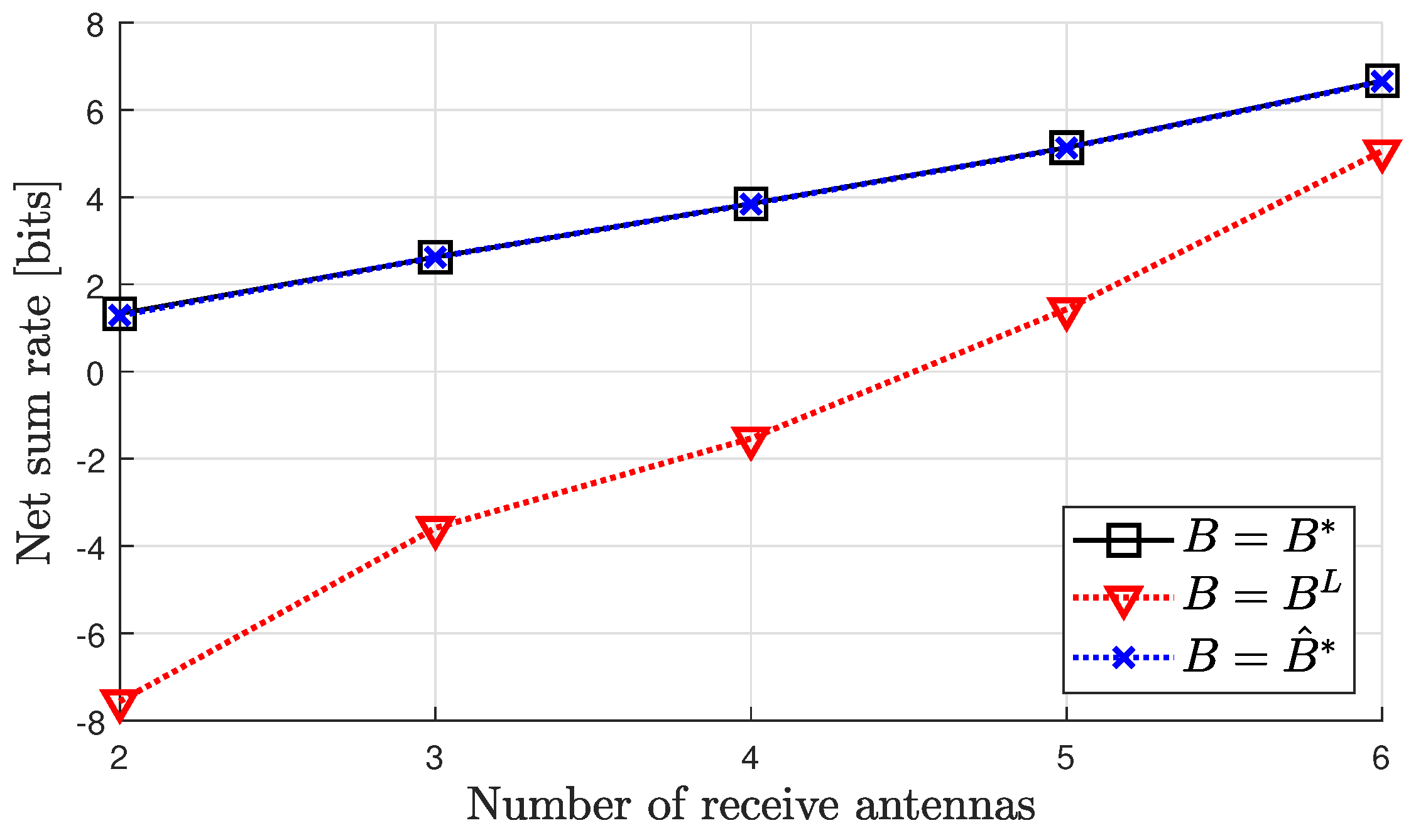
In this section, we present the simulation results to verify the accuracy of the estimate introduced in the preceding section. To facilitate the comparison, the following notations are employed:
  • As previously denoted, B * represents the optimal number of feedback bits in terms of maximizing R Net .
  • B ^ * signifies the proposed estimate derived by numerically approximating the rightmost zero crossing point of f Net , as outlined in Section Determination of the Optimal Feedback Rate.
  • B L stands for the lower bound of B * obtained in [12].
All results in this section are acquired through Monte Carlo simulations to obtain R Net , and a simulation guideline is provided as follows:
  • Initialization: Specify the values of the system parameters N t , N r , K, B, α , and μ . Fix the network’s radius to a sufficiently large value. For our results, we used a radius of 5 km for the entire network, and the values of α and μ are fixed as α = 4 and μ = 10 5 / π .
  • BS Locations: At each frame, determine the locations of BSs based on a Poisson point process. The number of BSs in the current frame follows a Poisson distribution with the corresponding density. Then, the BSs are uniformly distributed within a 2D circle.
  • User and channel setup: Assuming the target user is located at the origin, identify the BS closest to the origin as b 1 . Calculate the distances d i between the BSs and the target user. Generate small-scale fading channel matrices H k for k = 1 , , K , where components are i.i.d. circularly symmetric Gaussian with a variance of one. H k denotes the channel matrix between b i and user k { 1 , , K } , with user 1 as the target user. Note that, for simplicity, H 1 is denoted by H throughout this paper.
  • Quantization and precoding: Each user obtains H ^ k by quantizing H k in a distributed manner based on the QUB criterion described in Section 2.6. Construct precoding matrices V 1 , , V K using quantized channels, H ^ 1 , , H ^ K , collected from users, based on the BD criterion.
  • Inter-cell interference: Calculate matrices G i and F i , j following a similar approach used for obtaining H k and V k .
  • Net spectral efficiency: Compute the net spectral efficiency R Net at the current frame using Equations (6)–(8).
  • Monte Carlo simulation: Repeat steps (1)–(6) to obtain the ergodic average of the net spectral efficiency R Net .
All results were obtained using MATLAB on an inter-core i9 processor without the assistance of a GPU. The total number of frames used to derive R Net exceeds 50,000 for all simulations. In (36), the value of ϵ is set to 1 / 10 for all simulations following the results in [12].
Figure 1 and Figure 2 depict the optimal feedback bits varying with the coherent channel block length T c , considering two different setups of ( N t , N r , K ) . The black dashed line representing B * obtained through exhaustive search, while the blue dotted line indicates its analytical estimate, B ^ * , proposed in this paper. In accordance with our analysis in Section 3, the proposed estimate (dotted line) closely approximates the optimal number of feedback bits found through an exhaustive simulation. In contrast, the red solid lines depict two approximations proposed in [12], showing less accuracy when T c is relatively small (the discrepancy decreases as T c increases, consistent with the assumption of a large T c in the derivation of [12]). In summary, the proposed estimate in this study generally provides a much more accurate estimation compared to previous results.
Figure 3 directly compares the estimation errors of B ^ * and B L in estimating B * . The corresponding errors are depicted against the number of transmission antennas. As the number of transmission antennas increases, B * generally rises due to the increased requirement for feedback bits to attain a comparable CSIT accuracy for precoding. The bounds derived in previous studies, including B L , necessitate ‘sufficiently large’ feedback bits to closely approximate B * ; however, the range of ‘sufficiently large’ increases with N t since B * also increases with N t . Consequently, B L becomes less accurate with the increasing N t , and this trend is more pronounced when T c is smaller, as depicted in Figure 3. In contrast, the proposed estimate B ^ * generally maintains accuracy across varying N t .
In Figure 3, a noticeable amount of estimation error for the proposed estimate might be observed, especially for larger values of N t (e.g., when N t = 16 and T c = 100 ). However, around the optimal feedback bits, the rate of increase in R Net decreases as N t increases. Consequently, the estimation error of B ^ * depicted in Figure 3 remains tolerable regardless of N t , as illustrated in Figure 4. Remarkably, R Net at B ^ * and B * exhibit nearly identical values across varying N t , N r , and K, while the previously proposed lower bound B L demonstrates inaccurate approximation, particularly when T c is small. When considering the maximization of the net sum rate, our proposed estimate provides a much closer approximation to B * .
Simulation results show that the optimal number of feedback bits is quite large, especially when N t and N r have relatively large values. Thus, in practice, realizing such a huge codebook may be infeasible because the memory of a mobile device can be limited. Nevertheless, establishing a maximum achievable rate offers valuable insights into network operation during the design of corresponding wireless communication systems. It is important to note the substantial difference between designing a system with the knowledge of the performance upper bound and designing without such knowledge. In this context, we contend that our analysis results yield meaningful insights irrespective of the magnitude of the optimal B, even if the practical implementation of the entire optimal B value may pose challenges. While acknowledging that the optimal value of B may be too large for implementation by some network operators, they can still consider the increasing B as much as possible, given the awareness of the upper bound.

5. Conclusions

This paper maximized the net rate by analyzing the optimal feedback rate in a cellular network, where each BS implements BD and the network is modeled using stochastic geometry. To explore the optimal feedback bits, the analysis focused on studying the derivative of the net rate with respect to B. This derivative comprised two functions related to B, exhibiting different rates of increase. In contrast with prior studies, both functions were closely approximated using lower estimates. As a result, the overall estimate for the optimal feedback bits achieved near-optimal performance, irrespective of T c . Regarding the maximization of net spectral efficiency, the proposed estimate demonstrated a nearly identical performance compared to the true optimal value found from the exhaustive simulation. Furthermore, it provided significantly closer approximations than previous studies, especially for scenarios with a relatively small T c . Hence, the proposed estimate offers more accurate insights when designing limited-feedback-based precoding systems in dense cellular networks.

Author Contributions

Conceptualization, T.K. and M.M.; methodology, T.K. and M.M.; software, T.K. and M.M.; validation, T.K. and M.M.; formal analysis, T.K. and M.M.; investigation, T.K. and M.M.; resources, M.M.; data curation, T.K.; writing—original draft preparation, M.M.; writing—review and editing, T.K. and M.M.; visualization, T.K.; supervision, M.M.; project administration, M.M.; funding acquisition, M.M. All authors have read and agreed to the published version of the manuscript.

Funding

This work was supported in part by the National Research Foundation of Korea (NRF) grant funded by the Korea government (MSIT) (No. 2023R1A2C1004034), and in part by the BK21 FOUR Project funded by the Ministry of Education, Republic of Korea (4199990113966).

Data Availability Statement

Data is contained within the article.

Conflicts of Interest

The authors declare that there are no conflicts of interest.

Appendix A. Notations

Matrices are represented by uppercase bold letters, while column vectors are denoted by lowercase bold letters. The superscript ( · ) H signifies the complex conjugate transpose of a matrix. The symbol · denotes the vector norm, and | · | represents the absolute value of a complex number. The function Γ ( · ) stands for the Gamma function, Pr ( · ) indicates the probability of an event, E ( · ) represents the expectation, = d signifies equality in distribution, and d indicates approximation in distribution. The matrix I m is an m × m identity matrix. The sets N , R , and C denote the sets of natural numbers, real numbers, and complex numbers, respectively. β ( a , b ) represents the beta function with two parameters a and b.

Appendix B. Proof of Lemma 1

Given that X p is gamma-distributed with a shape N t N r and scale 1, we can express X p = d i = 1 N t N r G i , where G 1 , , G N t N r are i.i.d. random variables following a gamma distribution with shape 1 and scale 1. It is worth noting that a gamma distribution, characterized by a shape of 1 and a scale of 1, is equivalent to an exponential distribution with a mean of 1. Thus, (34) can be further calculated as
N r E X p ( N t N r ) + N r / ( A δ ) + Y p / ( A δ ) = N r ( N t N r ) E G 1 ( N t N r ) + N r / ( A δ ) + Y p / ( A δ ) = N r ( N t N r ) 0 Pr G 1 ( N t N r ) + N r / ( A δ ) + Y p / ( A δ ) > x d x = N r ( N t N r ) 0 Pr G 1 > x { ( N t N r ) + N r / ( A δ ) + Y p / ( A δ ) } d x = ( a ) N r ( N t N r ) 0 E e x { ( N t N r ) + N r / ( A δ ) + Y p / ( A δ ) } d x = N r ( N t N r ) 0 e ( N t N r + N r / ( A δ ) ) x · L Y p ( x / ( A δ ) ) d x ,
where ( a ) follows from the CDF of G 1 , and L Y p denotes the Laplace transform of Y p , i.e., L Y p ( t ) = E [ e t Y p ] . The computation of the right-hand side can be extended to
N r ( N t N r ) 0 e ( N t N r + N r / ( A δ ) ) x · L Y p ( x / ( A δ ) ) d x ( a ) N r ( N t N r ) h ( c , n ) 0 e ( N t N r + N r / ( A δ ) ) x ( x / ( A δ ) ) 2 α d x = N r ( N t N r ) ( A δ ) 2 α h ( c , n ) 0 e ( N t N r + N r / ( A δ ) ) x x 2 α d x = N r ( N t N r ) ( N t N r + N r / ( A δ ) ) 2 α 1 ( A δ ) 2 α h ( c , n ) 0 e z z 2 α d z = N r ( N t N r ) ( N t N r + N r / ( A δ ) ) 2 α 1 ( A δ ) 2 α h ( c , n ) Γ ( 1 2 α ) ,
where ( a ) is derived from the application of Lemma 1 in [10], and the subsequent equalities are obtained through the appropriate change of variables.

References

  1. Jindal, N. MIMO broadcast channels with finite-rate feedback. IEEE Trans. Inf. Theory 2006, 52, 5045–5060. [Google Scholar] [CrossRef]
  2. Yoo, T.; Jindal, N.; Goldsmith, A. Multi-antenna downlink channels with limited feedback and user selection. IEEE J. Sel. Areas Commun. 2007, 25, 1478–1491. [Google Scholar] [CrossRef]
  3. Renzo, M.D.; Guan, P. A mathematical framework to the computation of the error probability of downlink MIMO cellular networks by using stochastic geometry. IEEE Trans. Commun. 2014, 62, 2860–2879. [Google Scholar] [CrossRef]
  4. Renzo, M.D.; Lu, W. Stochastic geometry modeling and performance evaluation of MIMO cellular networks using the equivalent-in-distribution (EiD)-based approach. IEEE Trans. Commun. 2015, 63, 977–996. [Google Scholar] [CrossRef]
  5. Li, C.; Zhang, J.; Andrews, J.G.; Letaief, K.B. Success probability and area spectral efficiency in multiuser MIMO HetNets. IEEE Trans. Commun. 2016, 64, 1544–1556. [Google Scholar] [CrossRef]
  6. Lu, X.; Niyato, D.; Privault, N.; Jiang, H.; Wang, P. Managing Physical Layer Security in Wireless Cellular Networks: A Cyber Insurance Approach. IEEE J. Sel. Areas Commun. 2018, 36, 1648–1661. [Google Scholar] [CrossRef]
  7. Gao, Y.; Yang, S.; Wu, S.; Wang, M.; Song, X. Coverage probability analysis for mmWave communication network with ABSF-based interference management by stochastic geometry. IEEE Access. 2019, 7, 133572–133582. [Google Scholar] [CrossRef]
  8. Jia, X.; Ji, P.; Chen, Y. Modeling and analysis of multi-tier clustered millimeter-wave cellular networks with user classification for large-scale hotspot area. IEEE Access 2019, 7, 140278–140299. [Google Scholar] [CrossRef]
  9. Park, J.; Lee, N.; Andrews, J.G.; Heath, R.W., Jr. On the Optimal Feedback Rate in Interference-Limited Multi-Antenna Cellular System. IEEE Trans. Wireless Commun. 2016, 15, 5748–5762. [Google Scholar] [CrossRef]
  10. Min, M. Bounds on the Optimal Feedback Rate for Multi-Antenna Systems in Interference-Limited Cellular Networks. IEEE Trans. Wirel. Commun. 2018, 17, 4845–4860. [Google Scholar] [CrossRef]
  11. Sun, L.; Tian, X. Physical layer security in multi-antenna cellular systems: Joint optimization of feedback rate and power allocation. IEEE Trans. Wirel. Commun. 2022, 21, 7165–7180. [Google Scholar] [CrossRef]
  12. Lee, S.; Min, M. Analysis of the Optimal Feedback Rate for Limited Feedback-Based Block Diagonalization in Cellular MU-MIMO Systems. IEEE Wirel. Commun. Lett. 2023; Early Access. [Google Scholar] [CrossRef]
  13. Baccelli, F.; Blaszczyszyn, B. Stochastic Geometry and Wireless Networks: Volume I Theory; NOW Publishers: Norwell, MA, USA, 2009; Volume 3. [Google Scholar]
  14. Ravindran, N.; Jindal, N. Limited feedback-based block diagonalization for the MIMO broadcast channel. IEEE J. Sel. Areas Commun. 2008, 26, 1473–1482. [Google Scholar] [CrossRef]
  15. Andrews, J.G.; Baccelli, F.; Ganti, R.K. A tractable approach to coverage and rate in cellular networks. IEEE Trans. Commun. 2011, 59, 3122–3134. [Google Scholar] [CrossRef]
  16. Kang, Y.-S.; Min, M. Unified Derivation of Optimal Feedback Rate in Downlink Cellular Systems With Multi-Antenna Base Stations. IEEE Access. 2019, 7, 161871–161886. [Google Scholar] [CrossRef]
  17. Khatri, C.G. Classical statistical analysis based on a certain multivariate complex gaussian distribution. Ann. Math. Stat. 1965, 36, 98–114. [Google Scholar] [CrossRef]
  18. Gupta, A.; Nagar, D. Matrix Variate Distributions; Chapman & Hall/CRC: Boca Raton, FL, USA, 2000. [Google Scholar]
  19. Magnus, J.; Neudecker, H. Matrix Differential Calculus with Applications in Statistic and Econometrics; Wiley: Hoboken, NJ, USA, 1999. [Google Scholar]
Figure 1. B * and B ^ * vs. T c when N t = 8 , N r = 2 , K = 4 .
Mathematics 12 00460 g001
Figure 2. B * and B ^ * vs. T c when N t = 12 , N r = 3 , K = 3 .
Mathematics 12 00460 g002
Figure 3. Absolute error in estimating B * vs. N t when N r = 2 , K = N t / N r .
Mathematics 12 00460 g003
Figure 4. Net sum rate ( K R Net ( B ) ) vs. N r when N t = 20 , K = N t N r .
Mathematics 12 00460 g004
Disclaimer/Publisher’s Note: The statements, opinions and data contained in all publications are solely those of the individual author(s) and contributor(s) and not of MDPI and/or the editor(s). MDPI and/or the editor(s) disclaim responsibility for any injury to people or property resulting from any ideas, methods, instructions or products referred to in the content.

