A Matheuristic Approach for the Multi-Depot Periodic Petrol Station Replenishment Problem

Abstract

Planning petrol station replenishment is an important logistics activity for all the major oil companies. The studied Multi-Depot Periodic Petrol Station Replenishment problem derives from a real case in which the company must replenish a set of petrol stations from a set of depots, during a weekly planning horizon. The company must ensure refuelling according to available visiting patterns, which can be different from customer to customer. A visiting pattern predefines how many times (days) the replenishment occurs during a week and in which visiting days a certain amount of fuel must be delivered. To fulfill the weekly demand of each petrol station, one of the available replenishment plans must be selected among a given set of visiting patterns. The aim is to minimize the total distance travelled by the fleet of tank trucks during the entire planning horizon. A matheuristic approach is proposed, based on the cluster-first route-second paradigm, to solve it. The proposed approach is thoroughly tested on a set of realistic random instances. Finally, a weekly large real instance is considered with 194 petrol stations and two depots.

1. Introduction

The Petrol Station Replenishment Problem (PSRP) consists of finding optimal routes from a set of depots to replenish a set of petrol stations by using a fleet of tank trucks. Over recent decades, this problem has attracted the interest of many researchers and practitioners for its importance in the logistics of fuel oil distribution. As in this work, the study of the PSRP is often referred to in a real application case that is related to specific operative conditions imposed by petrol stations and oil companies. For this reason, there are various definitions and formulations of the problem that depend on the specific examined features. Most of the articles in the literature study the delivery problem from one depot to a set of petrol stations over a given planning horizon, or from multiple depots considering the 1-day variant of the problem. In our problem, the company has to deliver liquefied petroleum gas (LPG) from multiple depots and over a given planning horizon. Motivated by these real-life operative constraints, a multi-depot and periodic generalization of the PSRP is proposed: the Multi-Depot Periodic Petrol Station Replenishment Problem (MDPPSRP).

The MDPPSRP is only a part of the larger and more complex problem of planning the distribution of petrol products faced by an oil company. Usually, this problem is divided into three phases, depending on the specific planning horizon and constraints, which are strategic, tactical, and operational. In the strategic phase, concerning the long-term planning horizon (usually one year), the oil company assigns each refueling station to one or a few possible storage depots from which it will be replenished. In the operational phase, regarding the daily logistic activities, the final tank truck routes are defined, taking into account specific operational requirements such as the actual demand of distinct products (e.g., LPG, gasoline, diesel fuel) to be delivered to each petrol station for the specific day, possibly respecting a given time window and the characteristics of the tank trucks available in that day. During the (second) tactical phase, which is specifically considered in this paper, the medium-term (e.g., a few months or a season) fuel oil replenishment plans are defined for the petrol stations of a regional area (defined in the strategic phase). The days in which each petrol station will be replenished, as well as the depot from which the stations are served, are determined assuming the same demand every week for the entire period. Moreover, in this phase, the oil company is subject to several operative conditions and contract agreements with the petrol stations, which in general are not all owned by the company. For example, very often the oil company has to deal with small owners who have a limited budget for the purchase of petroleum products or limited storage capacity; the petrol station’s demand is then defined accordingly. For these reasons, each petrol station’s owner establishes one or multiple possible visiting patterns in which to be refueled during the week, in accordance with the oil company. A visiting pattern (options) predefines a set of replenishment (visiting) days and can be different from customer to customer.

The main aim in this tactical phase is to fulfill the estimated weekly demand of all petrol stations by selecting one of the available replenishment patterns for each petrol station and minimizing the total route length travelled by the tank trucks during the considered planning horizon.

The tactical problem described above can be modelled as a special case of the Multi-Depot Periodic Vehicle Routing Problem (MDPVRP). This problem extends the multi-depot version of the Capacitated VRP (CVRP), in which a set of clients must be served by a fleet of capacitated vehicles starting from different depots, by adding a time dimension and considering routes that will be performed over a planning horizon of p time periods (see, e.g., [1]). The CVRP is known to be NP-hard (see, e.g., Toth and Vigo [2]). Since the MDPVRP generalizes the CVRP, it is NP-hard too. A recent survey on the VRP and its variants can be found, for example, in Golden et al. [3].

However, the petrol distribution instances are profoundly different from the MDPVRP instances available from the literature, since in real applications, the ratio between the vehicle capacity and the average daily customer demand is very small (between 2 and 5) and, hence, feasible solutions are characterized by many daily routes, each one visiting a few petrol stations. Consequently, specific solving techniques should be required for the problem under consideration. In particular, a matheuristic approach is proposed, based on the cluster-first route-second paradigm to solve it. As mentioned before, for the specific problem considered, the number of visited stations in a route is very small and, for this reason, the attention is focused in detail on the clustering. Indeed, the petrol stations are grouped taking care of all the involved attributes and the specific operative constraints required by the company. Moreover, a specialized objective function to effectively solve the clustering phase is introduced.

Our contribution to the existing literature is as follows:

• Proposing an effective clustering model that takes care of all the involved attributes and considers the specific operative constraints required by the oil company.
• In the extensive computational study, the effectiveness of the clustering model is analyzed showing that the proposed solution method outperforms the meta-heuristic approach known in the literature.
• Experiments were carried out on instances of different sizes generated from a real case to analyze in detail the performance of the proposed approach. Finally, the heuristic is tested on a large instance with 194 petrol stations and two depots, considering a planning horizon of 6 days and 26 possible visiting patterns.

The remainder of this paper is organized as follows. In Section 2, a review of the relevant literature is provided; in Section 3, the addressed problem is formally defined and mathematically formulated. In Section 4, the proposed matheuristic approach is described, and the experimental analysis is reported in Section 5. Finally, the conclusion and the final discussion are in Section 6.

2. Literature Review

In this section, an updated review of the literature concerning the Petrol Station Replenishment Problem (PSRP) is presented, by focusing both on the main characteristics of the specific studied problems and on the methods proposed to solve them. The features considered in these problems are often highly specific and depend on the application and operative conditions imposed by the oil companies.

In any case, the main characteristics and constraints of the petrol station replenishment problem that are considered in the studied optimization models can be summarized as follows (see, e.g., [4,5]):

• Number of commodities: The company can distribute one or several types of products (e.g., LPG, gasoline, diesel fuel).
• Size of the fleet: Can be limited (fixed a priori) or can be one of the problem’s decision variables.
• Type of the fleet: Trucks may be identical (homogeneous fleet) or have different characteristics (heterogeneous fleet); furthermore, each truck, having a specific number of tanks (single-compartment or multi-compartment), can be equipped with flow meters, without which all the product loaded into a compartment cannot be used to replenish more than one station.
• Time windows: Petrol stations may require fuel replenishment in a specific time window.
• Number of depots: Products can be delivered from one or more depots; petrol stations can also be replenished from a subset of depots.
• Structure of the routes: Oil companies should consider constraints related to the maximum driving distance per truck, allowable working hours per day, and the maximum number of petrol stations to be served per day/route.
• Time horizon: Replenishment plans may cover a single day or a horizon of several working days (e.g., a week, in accordance with the visiting day chosen by the petrol stations).

Avella et al. [6] analyze a real case with 25 customers (petrol stations) served daily from the same depot by six heterogeneous multi-compartment tank trucks; to solve the problem, they proposed an exact approach using branch-and-price and a heuristic procedure. Ng et al. [7] provide a decision support system with the aim of finding the optimal fleet assignment and routing in two small distribution networks in Hong Kong. Also, in this case, the authors consider distributing different types of fuel oils with a fleet of heterogeneous trucks assigned at the same depot, evaluating multiple objectives simultaneously and solve the problem using a heuristic procedure.

In the same period, Cornillier et al. study several versions of the PSRP considering different purposes, constraints, and solution methods. In their first work [8], these authors propose an exact algorithm to assign the demand of a set of petrol stations to a given vehicle and design delivery routes to stations simultaneously. They solve the problem instances with both a homogeneous and a heterogeneous unlimited fleet of multi-compartment vehicles starting from a depot, under the operative constraint that at most two petrol stations are visited on each route. In their successive works, distinct models for different scenarios and related constraints are proposed with the aim of maximizing the total profit. They consider the problem with time window constraints and a limited heterogeneous fleet while assuming that up to four stations can be visited in a single route; for this case, they provide two heuristics. The first one is based on the arc preselection approach and the second one, used for larger instances, is based on the route preselection approach [9]. Finally, they extend these studies by providing a problem formulation and heuristic approaches to solve the multi-depot version of the problem with time windows [5].

The same constraints of the latter problem are considered by Benantar et al. [10] with the addition of vehicle accessibility constraints; indeed, they analyze a real scenario for an Algerian petroleum company that imposes a restriction on the assignment of vehicles to some petrol stations. Moreover, their objective is to minimize the sum of travelling costs and penalty costs. They provide a mathematical formulation, and they heuristically solve the problem with a tabu search (TS) algorithm. The same authors [11] extend their first study considering adjustable demands. Wang et al. [12] propose a model in which the trucks, homogeneous and with two compartments, can return several times to the depot and each petrol station has a time window according to the inventory. They develop a heuristic algorithm to solve the problem and evaluate the model using an instance based on real data gathered in Beijing. Wang et al. [13] introduce an adaptive large neighborhood search (ALNS) to solve a split-delivery version of the problem in which a petrol station can be replenished by multiple vehicles whenever a demand exceeds the vehicle capacity. The fleet consists of heterogeneous multi-compartment vehicles that, starting from a central depot, can execute multiple trips. Yahyaoui et al. [14] present an adaptive variable neighborhood search (AVNS) and a partially matched crossover PMX-based genetic algorithm to minimize the total travel distance of a homogeneous fleet of multi-compartment trucks. Che et al. [15] consider a multi-depot vehicle routing problem in which each depot can act as an intermediate replenishment facility (multi-depot VRP with open inter-depot routes). They formulated the problem as MILP and introduce a tabu-based adaptive large neighborhood search (T-ALNS) to solve it. Finally, Hajba et al. [16] propose a MILP model to solve the multi-compartment PSRP with time windows on a real case, applying a clustering method to reduce the complexity of the problem.

All the reviewed works mentioned above consider several aspects of the PSRP problem but, in all of them, only the 1-day variant of the problem is studied. Cornillier et al. [17] are among the first to analyze the multi-period problem with a limited fleet of heterogeneous tracks, several tanks, and a single depot. They approach this problem with a multi-phase heuristic, making use of the look-back and look-ahead procedures. Popović et al. [18] study a fuel oil distribution problem to minimize the total cost of the vehicle routing and inventory management. They proposed a variable neighborhood search (VNS) heuristic for solving a multi-product and multi-period inventory routing problem in fuel delivery. They consider a given deterministic petrol consumption for each petrol station and each fuel type, a homogeneous fleet of multi-compartment trucks, and a limit of three petrol stations visited in a route. Vidović et al. [19] extend this limit to four stations and propose two solution approaches: the resolution of a Mixed-Integer Programming (MIP) model via commercial solver, and a heuristics approach. The first one can be solved to optimality only for very small instances (with 10 petrol stations and 3 days); the second approach uses a relaxed MIP model to obtain an initial solution improved with a heuristic algorithm to solve instances with up to 50 petrol stations and a time horizon of 5 days.

A special case of the multi-period PSRP is the periodic version (PPSRP) that takes into account the periodic nature of the petrol station replenishment planning, where each petrol station i needs to be replenished $f_i$ days within a weekly time horizon and according to one of a set of available replenishment plans (visiting patterns) [4]. The single depot case of the PPSRP is studied by Triki [20] using a two-stage heuristic followed by a local search improvement procedure and by Carotenuto et al. [21,22] using a genetic and matheuristic approach, respectively. To the best of our knowledge, the only work that considers the multi-depot periodic version of the PSRP is the one proposed by Carotenuto et al. [23] in which the problem is solved using a hybrid genetic algorithm.

Finally, Al-Hinai and Triki [24] present a specific mathematical formulation to characterize the petrol replenishment market in the Sultanate of Oman, introducing the frequency service choice as a decision variable.

Table 1. Literature comparison. MP: periodic or multi-period; MT: multi-trip; MD: multi-depot.

	MP/MT	MD	Methods
Cornillier et al. [5]	MT	Yes	Matheuristic
Avella et al. [6]	-	No	Exact and Heuristic
Ng et al. [7]	-	No	Heuristic
Cornillier et al. [8]	-	No	Exact
Cornillier et al. [9]	MT	No	Matheuristic
Benantar et al. [10]	MT	No	Metaheuristic (TS)
Benantar et al. [11]	MT	No	Metaheuristic (TS)
Wang et al. [12]	MT	No	Heuristic
Wang et al. [13]	MT	No	Metaheuristic (ALNS)
Yahyaoui et al. [14]	MT	No	Metaheuristic (AVNS & GA)
Che et al. [15]	MT	Yes	Metaheuristic (T-ALNS)
Hajba et al. [16]	MT	No	Heuristic
Cornillier et al. [17]	MP	No	Heuristic
Popović et al. [18]	MP	No	Metaheuristic (VNS)
Vidović et al. [19]	MP	No	Metaheuristic (VNS)
Triki [20]	MP	No	Matheuristic
Carotenuto et al. [21]	MP	No	Metaheuristic (GA)
Carotenuto et al. [22]	MP	No	Matheuristic
Carotenuto et al. [23]	MP	Yes	Metaheuristic (GA)
Al-Hinai and Triki [24]	MP	No	Meta-heuristic
This paper	MP	Yes	Matheuristic

reports the main features of the problem considered in the literature and the type of solution procedures employed, dividing them into the exact method, heuristic, metaheuristic, or matheuristic. As reported in the table, most articles in the literature analyze the single-period version of the PSRP and the authors who face the multi-period case consider only one storage depot. To the best of our knowledge, this is the first paper that adopts a matheuristic approach and simultaneously solves the multi-depot and periodic petrol station replenishment problem.

In summary, compared to the only other article that considers the MDPPSRP, a different solution method based on the cluster-first route-second paradigm is introduced. In the clustering phase, the multi-depot and multi-period characteristics of the problem are considered simultaneously, obtaining clusters of petrol stations to be served during each day, each one assigned to a depot. In the clustering model, a specialized objective function to create effective clusters is introduced. Adopting this technique, sets of clusters of petrol stations are determined, whose total demand did not exceed the capacity of the vehicle, for which the corresponding Traveling Salesman Problem (TSP) is solved. Finally, the proposed approach outperforms the results obtained with a hybrid genetic algorithm in the only one article facing the multi-depot periodic version of the problem, by providing high-quality solutions in terms of effectiveness and efficiency.

3. Problem Description and Formulation

The Multi-Depot Periodic Petrol Station Replenishment Problem (MDPPSRP) consists of serving a set of petrol stations (customers) from a set of admissible depots. Each petrol station is assigned to one of its available replenishment plans (patterns) according to the required frequency of replenishment. To fulfill the selected replenishment plans, petrol stations are served by a fleet of homogeneous tank trucks (tankers) of capacity Q. Each one of them departs from an admissible depot, visits a subset of petrol stations, and returns to the same depot. The aim is to minimize the total distance traveled by the tankers during the planning horizon.

In more detail, referring to the classical PSRP characterization reported in the previous section, the problem that the company addresses can be characterized as follows:

• Number of commodities: Single commodity, petrol product consists of liquefied petroleum gas (LPG).
• Size of the fleet: To be determined to fulfill the petrol stations’ demand.
• Type of the fleet: Homogeneous fleet of single-compartment tank trucks.
• Time windows: No time windows are considered.
• Number of depots: Multiple depots are considered.
• Structure of the routes: Each truck may visit multiple petrol stations if their total demand does not exceed the tank truck capacity and each petrol station must be visited exactly once for each day of the selected replenishment pattern. No further limitations are considered for the truck routes.
• Time horizon: Planning horizon (week) composed of several time periods (days) in which each petrol station has a frequency of replenishment and a related demand per visit (equal for all the visiting days).

Finally, depending on operative conditions, the problem can be solved by allowing the replenishment of a petrol station from different depots on distinct visiting days (scenario Different Depot—DD) or, otherwise, only from the same depot for all the visiting days of the selected replenishment plan (scenario Same Depot—SD).

Table 2. Mathematical notation.

Sets:
C	set of petrol stations
D	set of storage depots
$D_i$	subset of admissible depots for petrol station $i\in C$, $D_i\subseteq D$
N	set of nodes, $N=D\cup C$
A	set of arcs, $A=\left\{\right(i,j)\in N\times N:i\ne j\}$
T	set of time periods (days) of the planning horizon
$\Pi$	set of (all) replenishment patterns
${\Pi }_i$	subset of replenishment patterns with frequency $f_i$ for petrol station $i\in C,{\Pi }_i\subseteq \Pi$
Parameters:
$c_{ij}$	travel distance from i to j, with $(i,j)\in A$
$a_{\pi t}$	binary parameter equal to 1 if replenishment pattern $\pi \in \Pi$ requires a visit in time period $t\in T$, and 0 otherwise
Q	tank truck capacity
$d_i$	periodic demand of petrol station $i\in C$
Variables:
$x_{ijot}$	binary decision variables equal to 1 if arc $(i,j)\in A$ is traversed in time period $t\in T$ by a route starting from depot $o\in D$, and 0 otherwise
$y_{i\pi }$	binary decision variables equal to 1 if petrol station $i\in C$ is replenished with replenishment plan $\pi \in {\Pi }_i$, and 0 otherwise
$y_{io\pi }$	binary decision variables equal to 1 if petrol station $i\in C$ is replenished with replenishment plan $\pi \in {\Pi }_i$ with all routes starting from depot $o\in D_i$, and 0 otherwise
$u_{iot}$	continuous variable representing the total amount of fuel oil delivered after having visited petrol station $i\in C$ with a vehicle route starting from depot $o\in D_i$ at time period $t\in T$

lists the notation used in the remainder of the paper.

Considering the above assumptions and assuming that the route that visits customer i must start from depot $o\in D_i\subseteq D$, two models that take into account the specific operative conditions coming from the real case that characterize the assignment of depots to petrol stations are reported. When the assignment of different depots to a petrol station in distinct time periods is allowed (scenario DD), the two indices assigning variable $y_{i\pi }$ are used and the problem can be formulated with the following vehicle flow model, where $x_{ijot}$ variables related to arc $(i,j)$ can be regarded as arc flow variables (see, e.g., Toth and Vigo [2]):

$$minz=\sum _{(i,j)\in A}\sum _{o\in D}\sum _{t\in T}{c}_{ij}{x}_{ijot}$$

(1)

s.t.

$$\begin{array}{cccc}\hfill & \sum _{\pi \in {\Pi }_i}{y}_{i\pi }=1\hfill & \hfill & \forall i\in C\hfill \end{array}$$

(2)

$$\begin{array}{cccc}\hfill & \sum _{o\in D_i}\sum _{j\in C\cup \left\{o\right\}:(i,j)\in A}{x}_{ijot}=\sum _{\pi \in {\Pi }_i}{a}_{\pi t}{y}_{i\pi }\hfill & \hfill & \forall i\in C,t\in T\hfill \end{array}$$

(3)

$$\begin{array}{cccc}\hfill & \sum _{h\in N:(h,i)\in A}{x}_{hiot}+\sum _{j\in N:(i,j)\in A}{x}_{ijot}=0\hfill & \hfill & \forall i\in C,o\in D\setminus D_i,t\in T\hfill \end{array}$$

(4)

$$\begin{array}{cccc}\hfill & \sum _{h\in C\cup \left\{o\right\}:(h,i)\in A}{x}_{hiot}=\sum _{j\in C\cup \left\{o\right\}:(i,j)\in A}{x}_{ijot}\hfill & \hfill & \forall i\in C,o\in D_i,t\in T\hfill \end{array}$$

(5)

$$\begin{array}{cccc}\hfill & \sum _{i\in C:(i,o)\in A}{x}_{ioot}=\sum _{j\in C:(o,j)\in A}{x}_{ojot}\hfill & \hfill & \forall o\in D,t\in T\hfill \end{array}$$

(6)

$$\begin{array}{cccc}\hfill & u_{iot}-u_{jot}+Q{x}_{ijot}\le Q-d_j\sum _{\pi \in {\Pi }_j}{a}_{\pi t}{y}_{j\pi }\hfill & \hfill & \forall i,j\in C:(i,j)\in A,o\in D_i\cap D_j,t\in T\hfill \end{array}$$

(7)

$$\begin{array}{cccc}\hfill & d_i\sum _{\pi \in {\Pi }_i}{a}_{\pi t}{y}_{i\pi }\le u_{iot}\le Q\hfill & \hfill & \forall i\in C,o\in D_i,t\in T\hfill \end{array}$$

(8)

$$\begin{array}{cccc}\hfill & y_{i\pi }\in \{0,1\}\hfill & \hfill & \forall i\in C,\pi \in \Pi \hfill \end{array}$$

(9)

$$\begin{array}{cccc}\hfill & x_{ijot}\in \{0,1\}\hfill & \hfill & \forall (i,j)\in A,o\in D,t\in T\hfill \end{array}$$

(10)

The objective function (1) minimizes the total travel distance. Constraints (2) ensure that exactly one replenishment plan is assigned to each petrol station. Constraints (3) guarantee that the customer visits occur only on the time periods specified by the assigned replenishment plan. Constraints (4) ensure that each petrol station is served from an admissible depot. Constraints (5) and (6) guarantee the flow conservation for each petrol station and depot, respectively. Constraints (7) and (8) represent subtour elimination and tank truck capacity constraints. These constraints are derived from the subtour elimination constraints proposed by Kara et al. [25] for the capacitated VRP and extended to the multi-depot and multi-period case. Finally, constraints (9) and (10) define the domains of the decision variables.

Given a solution $(\overline{x},\overline{y},\overline{u})$, the total number of generated routes for the whole planning horizon (week) is equal to ${\sum }_{t\in T}{\sum }_{o\in D}{\sum }_{j\in C:(o,j)\in A}{\overline{x}}_{ojot}$. Assuming that a truck can be used at most once for each period (day) $t\in T$ and that it cannot be transferred in another depot at the end of each period, the total number of used trucks will be equal to ${\sum }_{o\in D}{max}_{t\in T}\left\{{\sum }_{j\in C:(o,j)\in A}{\overline{x}}_{ojot}\right\}$.

If the operative conditions require that each petrol station is replenished always from the same depot during the entire planning horizon (scenario SD), the three-index binary variable $y_{io\pi }$ is used, in place of the two-index binary variable $y_{i\pi }$, to represent the assignment of depot $o\in D_i$ and replenishment pattern $\pi \in {\Pi }_i$ to petrol station $i\in C$. The problem is formulated with the above formulation (1)–(10), except for constraints (2), (3), (7), and (8), which are replaced with constraints (11)–(14), respectively:

$$\begin{array}{cccc}\hfill & \sum _{o\in D_i}\sum _{\pi \in {\Pi }_i}{y}_{io\pi }=1\hfill & \hfill & \forall i\in C\hfill \end{array}$$

(11)

$$\begin{array}{cccc}\hfill & \sum _{j\in C\cup \left\{o\right\}:(i,j)\in A}{x}_{ijot}=\sum _{\pi \in {\Pi }_i}{a}_{\pi t}{y}_{io\pi }\hfill & \hfill & \forall i\in C,o\in D_i,t\in T\hfill \end{array}$$

(12)

$$\begin{array}{cccc}\hfill & u_{iot}-u_{jot}+Q{x}_{ijot}\le Q-d_j\sum _{k\in D_j}\sum _{\pi \in {\Pi }_j}{a}_{\pi t}{y}_{jk\pi }\hfill & \hfill & \forall i,j\in C:(i,j)\in A,o\in D_i\cap D_j,t\in T\hfill \end{array}$$

(13)

$$\begin{array}{cccc}\hfill & d_i\sum _{k\in D_i}\sum _{\pi \in {\Pi }_i}{a}_{\pi t}{y}_{ik\pi }\le u_{iot}\le Q\hfill & \hfill & \forall i\in C,o\in D_i,t\in T\hfill \end{array}$$

(14)

Constraints (11) ensure that exactly one replenishment plan and one depot are assigned to each petrol station. Constraints (12) guarantee that for each petrol station, the visits, always starting from the assigned depot, occur only on the time periods specified by the selected replenishment plan. Finally, constraints (13) and (14) correspond to subtour elimination and capacity constraints, respectively.

4. Heuristic Procedures

Due to the large size of the real instances we wish to solve, the MDPPSRP is solved heuristically to find good solutions in reasonable time. In particular, the characteristics of the problem lead to solving it with a two-phase approach, subdividing the problem into a replenishment planning phase and a routing phase. In the first (clustering) phase, one replenishment plan (visiting pattern) is selected for each petrol station, i.e., it is determined when (in which periods) the petrol stations will be replenished, and petrol stations to be served in the same period are clustered into small groups of nearby depot and petrol stations whose total demand is not greater than the truck capacity. In the second (routing) phase, the best route is finally found for serving each group of petrol stations from the assigned depot by a single truck, by solving the related TSP instance. The novelty of the proposed approach is that the clustering model is able to provide a good approximation of the value of the whole solution obtained after the routing phase.

The solutions of both phases are obtained by solving the related mathematical model. The entire procedure can be summarized as follows:

Ph.1

Solve the following clustering model. For each petrol station $i\in C$, select exactly one of the available replenishment patterns ${\Pi }_i$, and, for each period $t\in T$ of the planning horizon, group petrol stations to be served in period t into clusters of total demand at most equal to Q and assign each cluster to a depot $o\in D$.

Ph.2

Solve a TSP instance for each cluster of petrol stations assigned to a depot, according to the solution of clustering model obtained in Ph.1.

The clustering model used in this first phase is as follows. A set V of petrol stations’ virtual centers is considered, and for simplicity, it is assumed that the positions of the centers are chosen among those of the set of petrol stations; therefore, $V=C$. The problem addressed in the clustering stage consists of selecting exactly one of the available replenishment plans (visiting patterns), for each petrol station, and assigning petrol stations to centers. Given the assignment of replenishment plans to petrol stations, for each day $t\in T$ in which a station is visited, a center and an available depot are assigned to it. It is guaranteed that the total demand of the petrol stations assigned in day t to the same couple of center and depot is not greater than the truck capacity. The following binary variables are introduced. $h_{jot}$ equals 1 if the virtual center $j\in V$ is activated and assigned to depot $o\in D$ in time period $t\in T$, and 0 otherwise; $w_{ijot}$ equals 1 if petrol station $i\in C$ is assigned to virtual center $j\in V$ and is activated and assigned to depot $o\in D_i$ in time period $t\in T$, and 0 otherwise.

To estimate as much as possible the total route distance traveled by the tank trucks visiting the groups of petrol stations, the following objective function is considered:

$$z=\sum _{o\in D}\sum _{j\in V}\sum _{t\in T}(c_{oj}+c_{jo})h_{jot}+\sum _{i\in C}\sum _{o\in D}\sum _{j\in V}\sum _{t\in T}\frac{1}{2}[(c_{ij}+c_{ji})+(c_{io}+c_{oi})-(c_{jo}+c_{oj})]w_{ijot}$$

(15)

The objective function consists of two terms. The first one is used to evaluate the total round-trip distance to the virtual centers from their respective assigned depot; the second term is used to estimate the additional total distance to serve the petrol stations assigned to the virtual centers. In more detail, the second term of the objective function is evaluated assuming a visit to a petrol station diverting as little as possible from the main route depot-virtual center-depot. To evaluate the additional distance, the mean distance between three pairs of nodes is considered: petrol station-virtual center, petrol station-depot, and depot-virtual center; the first two amounts are summed and then the last one is subtracted. According to the two scenarios (DD, SD) described in the previous section, two related models are introduced. The first one, in which a petrol station can be served from different depots during the planning horizon (scenario DD), can be formulated as follows:

$$minz=\sum _{o\in D}\sum _{j\in V}\sum _{t\in T}(c_{oj}+c_{jo})h_{jot}+\sum _{i\in C}\sum _{o\in D}\sum _{j\in V}\sum _{t\in T}\frac{1}{2}[(c_{ij}+c_{ji})+(c_{io}+c_{oi})-(c_{jo}+c_{oj})]w_{ijot}$$

(16)

s.t.

$$\begin{array}{cccc}\hfill & \sum _{\pi \in {\Pi }_i}{y}_{i\pi }=1\hfill & \hfill & \forall i\in C\hfill \end{array}$$

(17)

$$\begin{array}{cccc}\hfill & \sum _{j\in V}\sum _{o\in D_i}{w}_{ijot}=\sum _{\pi \in {\Pi }_i}{a}_{\pi t}{y}_{i\pi }\hfill & \hfill & \forall i\in C,t\in T\hfill \end{array}$$

(18)

$$\begin{array}{cccc}\hfill & \sum _{o\in D}{h}_{jot}\le 1\hfill & \hfill & \forall j\in V,t\in T\hfill \end{array}$$

(19)

$$\begin{array}{cccc}\hfill & \sum _{i\in C}\sum _{o\in D_i}{d}_i{w}_{ijot}\le Q\sum _{o\in D}{h}_{jot}\hfill & \hfill & \forall j\in V,t\in T\hfill \end{array}$$

(20)

$$\begin{array}{cccc}\hfill & w_{ijot}\le h_{jot}\hfill & \hfill & \forall i\in C,j\in V,o\in D_i,t\in T\hfill \end{array}$$

(21)

$$\begin{array}{cccc}\hfill & y_{i\pi }\in \{0,1\}\hfill & \hfill & \forall i\in C,\pi \in {\Pi }_i\hfill \end{array}$$

(22)

$$\begin{array}{cccc}\hfill & h_{jot}\in \{0,1\}\hfill & \hfill & \forall j\in V,o\in D,t\in T\hfill \end{array}$$

(23)

$$\begin{array}{cccc}\hfill & w_{ijot}\in \{0,1\}\hfill & \hfill & \forall i\in C,j\in V,o\in D_i,t\in T\hfill \end{array}$$

(24)

Constraints (17) assure that exactly one replenishment plan (pattern) is assigned to each petrol station. Constraints (18) assign exactly one center and one depot to each petrol station for each day belonging to the selected replenishment plan. Constraints (19) assure that at most one depot can be assigned to a center activated for a given day of the planning horizon. Constraints (20) limit the total demand of the petrol stations assigned to a given virtual center activated on a specific day to be at most equal to the tank truck capacity. Constraints (21) imply that a petrol station can be assigned to an admissible depot and a virtual center in a given day of the planning horizon only if that center is activated in that day and assigned to that depot. Finally, constraints (22)–(24) define the domains of the decision variables.

To model the scenario in which each petrol station should be replenished from the same depot during the whole planning horizon (scenario SD), the three-index binary variable $y_{io\pi }$ is used in place of the two-index binary variable $y_{i\pi }$, and we replace constraints (17) and (18) with the following ones, respectively:

$$\begin{array}{cccc}\hfill & \sum _{o\in D_i}\sum _{\pi \in {\Pi }_i}{y}_{io\pi }=1\hfill & \hfill & \forall i\in C\hfill \end{array}$$

(25)

$$\begin{array}{cccc}\hfill & \sum _{j\in V}{w}_{ijot}=\sum _{\pi \in {\Pi }_i}{a}_{\pi t}{y}_{io\pi }\hfill & \hfill & \forall i\in C,o\in D_i,t\in T\hfill \end{array}$$

(26)

Constraints (25) ensure that exactly one replenishment plan and one depot are assigned to each petrol station for the whole planning horizon. Constraints (26) guarantee that exactly one virtual center is assigned to each petrol station along with the selected depot, for each day belonging to the selected replenishment plan.

The result of the clustering phase is therefore a partition of the set of petrol stations to be served during each day into subsets of total demand of at most Q, each one assigned to a depot. Given a solution $(\overline{y},\overline{h},\overline{w})$ of the clustering model, the total number of generated clusters is equal to ${\sum }_{o\in D}{\sum }_{j\in V}{\sum }_{t\in T}{\overline{h}}_{jot}$.

In the routing phase, an optimal tour is determined for each cluster of petrol stations starting from and returning to the assigned depot, by solving the related TSP instance. Moreover, due to the tank truck capacity and petrol station demands, the number of petrol stations to be replenished by a tank truck is typically very small in real instances (on average three, and at most five) and, hence, the TSP can be solved optimally in a very short time, by solving exactly one of the classical well-known TSP mathematical formulations (see, e.g., Dantzig et al. [26], Miller et al. [27]). Denote with $z^c\left(M\right)$ the best solution value of the clustering phase of model $M=\{DD,SD\}$, and with $z\left(M\right)$ the final solution value (total routing length) provided by the clustering–routing approach.

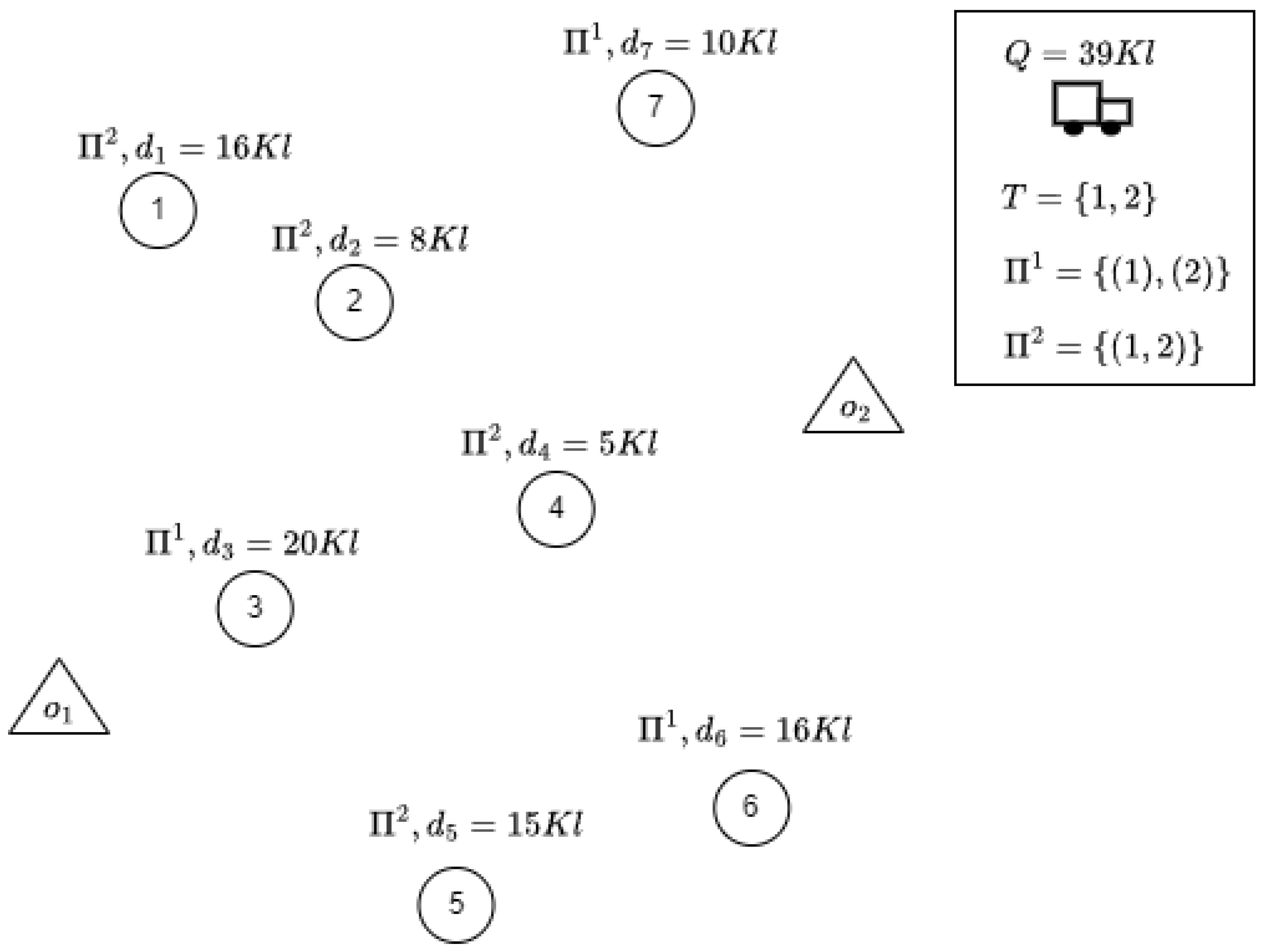
To better illustrate the heuristic procedure, a small example with seven petrol stations and two depots shown in Figure 1 is discussed, where petrol stations are represented by circles numbered from 1 to 7, and the two depots $o_1$ and $o_2$ by triangles. Moreover, a planning horizon T of two periods (days) and two replenishment patterns with a single (${\Pi }^1$) or double (${\Pi }^2$) frequency of service are considered. Finally, the truck capacity (Q) is equal to 39 Kl.

For each petrol station, the visiting pattern and the demand are reported in the figure. For example, petrol station 1 requires two visits (one for each period), each one with 16 Kl of LPG, while petrol station 3 requires 20 Kl of LPG in a single visit (to be carried out in one of the two periods).

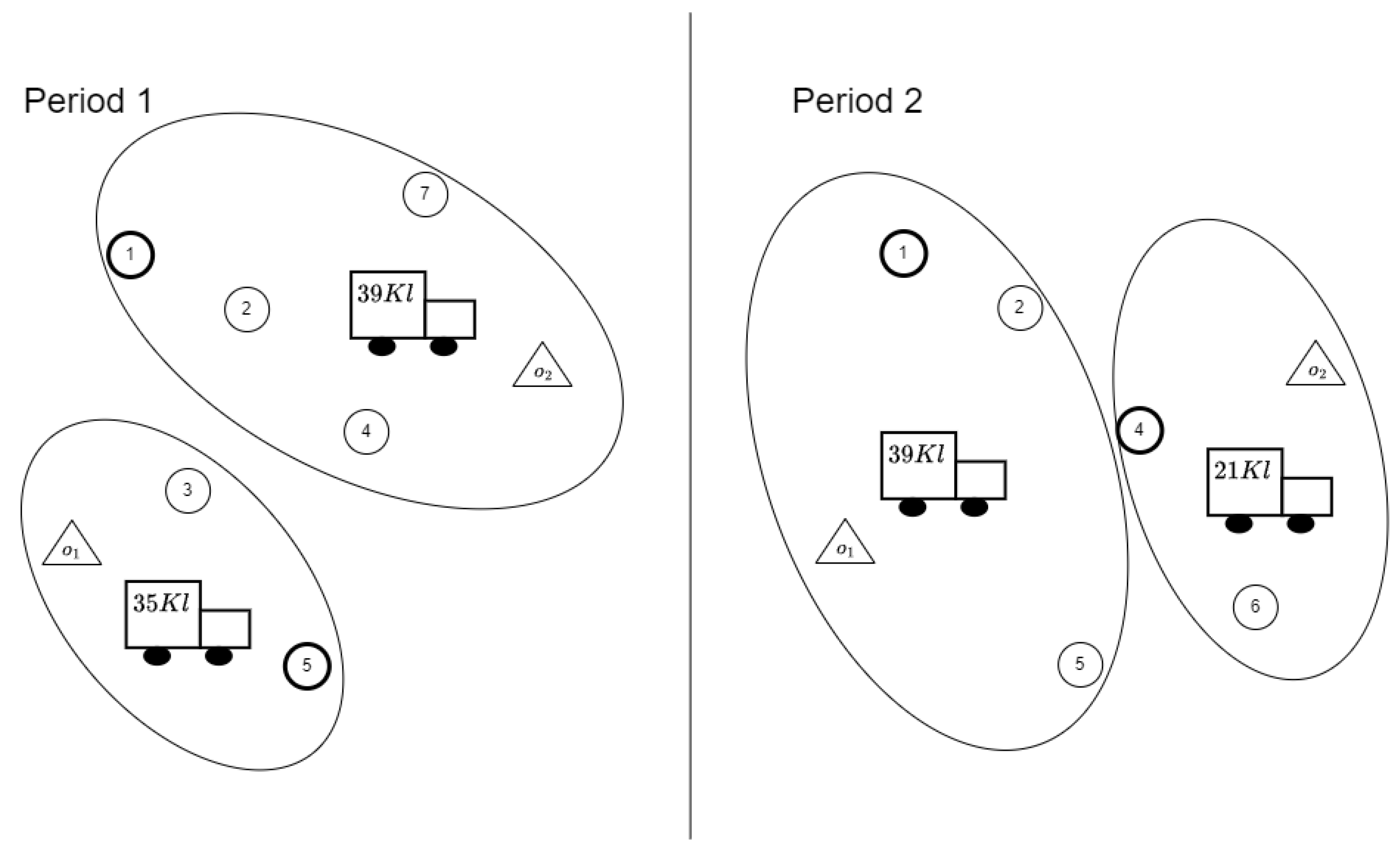
Considering scenario DD, the solution of the first phase returns four clusters, as shown in Figure 2 (reported as oval, with the related virtual centers in bold). In each cluster, a subset of petrol stations to be visited by a truck are grouped, according to the petrol station replenishment patterns and the truck capacity. In particular, for each one of the two periods, two clusters are generated; for example, in period 1, a cluster groups depot $o_1$ and petrol stations 3 and 5 with a total LPG demand of $35Kl$, and the other one groups depot $o_2$ and petrol stations 1, 2, 4, and 7 (with total demand $39Kl$). Since it is assumed that each truck can be used in different periods but always departing from the same depot, and that it can be used at most once for each period, in this example, the total number of used trucks will be equal to 2.

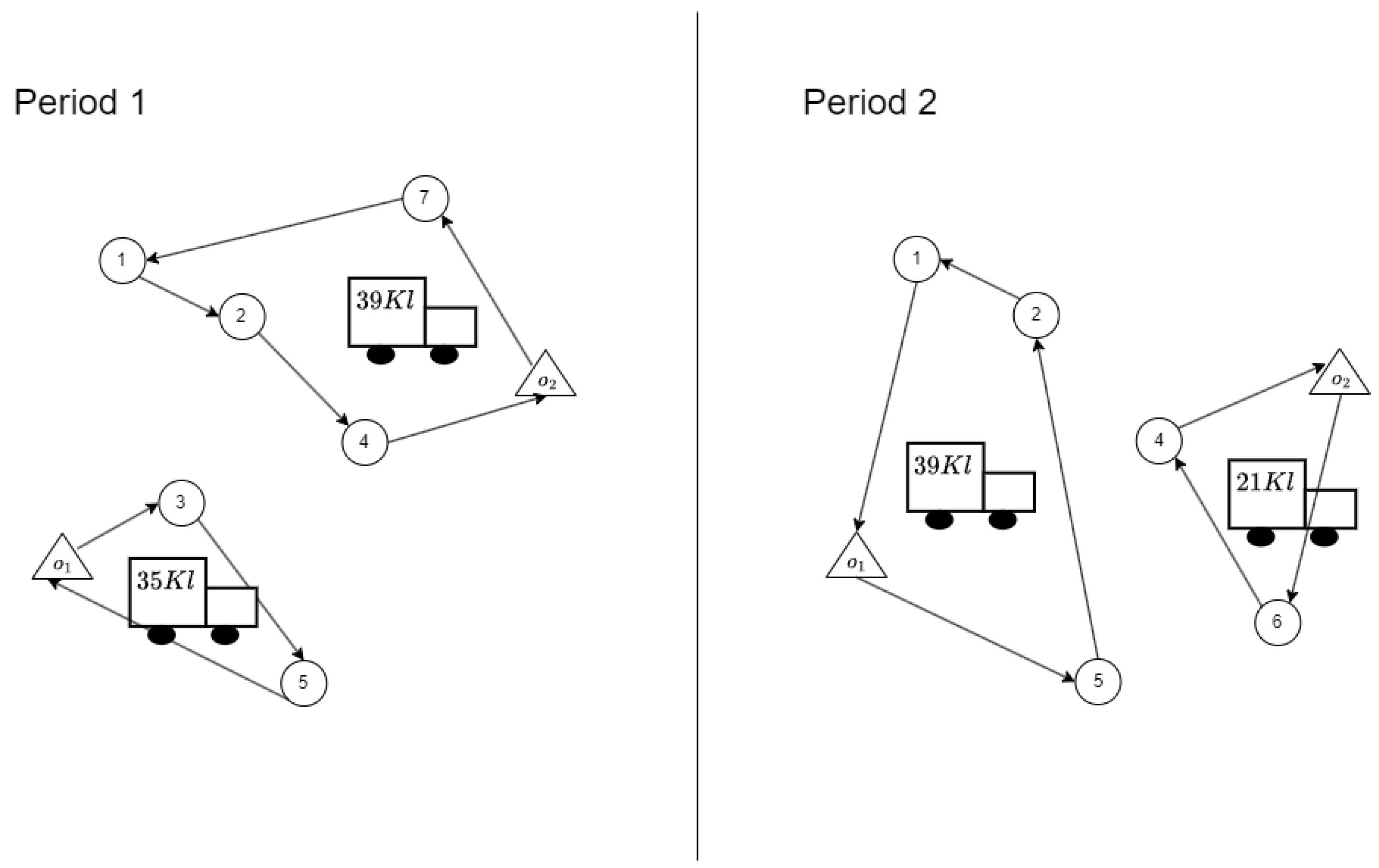
As shown in Figure 3, for each one of the four clusters determined in phase 1, a TSP is solved optimally to obtain the petrol station visiting sequence performed by a truck and the related length traveled. Finally, their sum gives the total length traveled by the fleet during the planning horizon.

According to scenario DD, petrol station 2 is served from depot $o_2$ in period 1 and from depot $o_1$ in period 2. By solving the same instance for scenario SD, a different clusterization will be obtained, with petrol station 2 assigned to the same depot ($o_1$) in both periods.

5. Computational Experiment

The proposed two-phase approach was implemented in AMPL using Gurobi 8.1.0 as the MILP solver and run on a PC with an Intel Core i3 2.30 GHz CPU and 4 GB of RAM. To assess the performance of this approach, it is tested on 45 random instances generated from a large real case instance of an oil company already considered in Carotenuto et al. (2018). The real instance has two depots and 194 petrol stations (196 nodes) that require weekly a total amount of 4783 kiloliters (kl) of fuel (LPG), with demands ranging between 3 kl and 38 kl per visit. Tank truck capacity Q is equal to 39 kl.

5.1. Dataset

A (weekly) planning horizon composed of 6 time periods (days) is considered. During this planning horizon, each petrol station i, in accordance with the company, specifies the frequency of service $f_i$, ranging from 1 (i.e., a single weekly visit) to 6 (i.e., a daily service).

Table 3. Visiting patterns.

Frequency of Service, f	Visiting Patterns, ${\mathsf{\Pi }}^{\mathit{f}}$
1	${\Pi }^1$ = {(1), (2), (3), (4), (5), (6)}
2	${\Pi }^2$ = {(1, 3), (1, 4), (1, 5), (2, 4), (2, 5), (2, 6), (3, 5), (3, 6)}
3	${\Pi }^3$ = {(1, 2, 4), (1, 2, 5), (1, 3, 5), (1, 4, 5), (2, 4, 5), (2, 4, 6)}
4	${\Pi }^4$ = {(1, 2, 4, 5), (1, 2, 4, 6), (2, 3, 4, 6)}
5	${\Pi }^5$ = {(1, 2, 3, 4, 5), (1, 2, 3, 4, 6)}
6	${\Pi }^6$ = {(1, 2, 3, 4, 5, 6)}

lists the set ${\Pi }^f$ of visiting patterns of frequency f, with $f=1,\dots ,6$. For example, referring to this table, a petrol station i requiring service three times a week (i.e., $f_i=3$) will be replenished during days ${\tau }_1$, ${\tau }_2$, and ${\tau }_3$, according to the selected 3-tuple (${\tau }_1$, ${\tau }_2$, ${\tau }_3$) out of the six available ones of visiting pattern set ${\Pi }^3$. The amount of fuel to be delivered to the petrol station i for each visiting day is the same and equal to $d_i$.

Realistic random instances are generated starting from the real case. Firstly, 10 small instances of 12 nodes, 10 petrol stations, and two depots are generated. Then, the experimental analysis proceeds by testing 10 instances of 150, 100, 50, and 20 nodes; 148, 98, 48, and 18 petrol stations have been randomly selected from the 194 petrol stations of the real case instances. The two depots, the replenishment frequencies, and the demand quantities have been preserved as in the real case.

The proposed models are tested considering different CPU time limits; since all the TSP instances of the routing phase are solved to optimality with negligible time, the time limits are considered only for the clustering phase. A thorough experimental analysis is discussed in the following subsections. Firstly, the effectiveness of the proposed clustering-first route-second modelling approach is evaluated with respect to the solutions provided by Gurobi for the exact model; this analysis is carried out only on very small instances for which Gurobi is able to find approximate solutions for this model in a reasonable time. Subsequently, the relationship is analyzed between the solution values obtained after the first clustering phase and after the second routing phase in order to evaluate the effectiveness of the clustering models on the estimation of the final solution values. Moreover, the performance of the clustering models is analyzed by evaluating the impact of the CPU time limit on the quality of the final obtained solutions. Finally, the proposed approach is tested on the real instance with 194 petrol stations.

5.2. Comparison with the Exact Model

The first testing phase regards the comparison of the proposed approach with the exact model on a set of very small instances with 12 nodes (10 petrol stations and two depots), for which the exact model can be solved optimally by Gurobi within 2 h (7200 s) for both scenarios.

Table 4. Exact model results: 10 petrol stations and 2 depots (12 nodes), and 6 periods. Results of the exact model solved with Gurobi within 2 h. $z^{*}\left(EM\right)$: value of the optimal solution obtained with the exact model; $z\left(M\right)$: solution values provided by the heuristic approach; ${\Delta }_{EM}$: percentage deviation between $z^{*}\left(EM\right)$ and $z\left(M\right)$.

	Scenario DD					Scenario SD
Instance	${\mathit{z}}^{*}\left(\mathit{EM}\right)$	Time (s)	$\mathit{z}\left(\mathit{DD}\right)$	Time (s)	${\Delta }_{\mathit{EM}}(\%)$	${\mathit{z}}^{*}\left(\mathit{EM}\right)$	Time (s)	$\mathit{z}\left(\mathit{SD}\right)$	Time (s)	${\Delta }_{\mathit{EM}}(\%)$
12_1	1213.24	403.12	1213.26	0.12	0.00	1213.24	1035.44	1213.24	0.24	0.00
12_2	2226.99	73.54	2226.99	0.81	0.00	2268.03	10.91	2268.03	1.97	0.00
12_3	1720.76	4146.18	1720.77	1.23	0.00	1720.76	4025.93	1720.77	1.27	0.00
12_4	2468.94	2817.42	2483.63	3.15	0.59	2513.06	33.73	2513.06	23.45	0.00
12_5	2796.18	613.48	2826.03	2.79	1.07	2848.81	190.22	2850.11	4.20	0.05
12_6	1797.13	168.37	1810.72	0.33	0.76	1797.13	5.98	1810.72	0.26	0.76
12_7	3179.42	20.95	3179.42	0.67	0.00	3179.42	20.38	3179.42	0.70	0.00
12_8	3177.12	482.81	3177.12	0.65	0.00	3177.12	537.24	3177.12	0.59	0.00
12_9	1783.11	68.29	1783.11	0.63	0.00	1783.11	8.61	1783.11	0.75	0.00
12_10	1835.04	49.54	1835.04	0.15	0.00	1835.04	8.25	1835.04	0.11	0.00
Average		884.37		1.05	0.24		587.67		3.35	0.08

lists the solution values and the computational time (in seconds) provided by the exact model ($z^{*}\left(EM\right)$) and with the heuristic approach ($z\left(M\right)$), for scenarios DD and SD. Moreover, the percentage deviation, evaluated as ${\Delta }_{EM}=100\frac{z\left(M\right)-z^{*}\left(EM\right)}{z^{*}\left(EM\right)}\%$, between the two approaches is reported. Finally, the average computational time and the average deviation values are listed in the last row of the table.

For all these instances, the solver obtains the optimal solution, but despite the small number of petrol stations considered, it spends on average 884 s and 587 s to solve the instances in scenarios DD and SD, respectively. The proposed heuristic approach provides the same optimal results in a few seconds on seven out of ten instances in scenario DD, with an average (max) gap of $0.24\%$ ($1.07\%$), and on eight out of ten instances in scenario SD, with an average (max) gap of $0.08\%$ ($0.76\%$). These results highlight the goodness of the proposed approach both in terms of effectiveness (with respect to the optimal solution values) and efficiency (in comparison with the exact model).

To further point out the need of a heuristic approach to solve these types of instances, the analysis continues by increasing the number of nodes to 20 (18 petrol stations and two depots). Also, despite the fact that these instances are quite small, the Gurobi solver was not able to solve the exact model (EM) for any instance to optimality within 48 h; moreover, on average, the gap between the returned solution and the best computed lower bound was quite large. Therefore, these results show the need for a heuristic approach to solve small and larger realistic instances of the MDPPSRP.

For each one of the 10 small instances,

Table 5. Exact model results: 18 petrol stations and 2 depots (20 nodes), and 6 periods. Results of the exact model solved with Gurobi within 48 h. $z\left(EM\right)$: value of the best solution obtained; $LB$: lower bound calculated by the solver; gap%: gap in percentage between $z\left(EM\right)$ and $LB$.

Instance	$\mathit{z}\left(\mathit{EM}\right)$ (km)	$\mathit{LB}$ (km)	gap%
20_1	1391.98	1224.11	12.10%
20_2	2940.20	2661.51	9.48%
20_3	2016.74	1331.28	34.00%
20_4	2747.36	2233.77	18.70%
20_5	3283.15	3049.73	7.11%
20_6	2182.10	1552.75	28.80%
20_7	2313.26	1275.48	44.90%
20_8	4066.49	3322.71	18.30%
20_9	2526.63	1677.59	33.60%
20_10	2118.79	1879.90	11.30%

lists the total route length $z\left(EM\right)$ obtained by solving the exact model for scenario DD, i.e., model (1)–(10), within the given time limit, the best lower bound LB calculated by the solver, and the gap in percentage between them, evaluated as gap% $=100(1-\frac{LB}{z\left(EM\right)})\%$. Analog results were also obtained for scenario SD with its specific model.

On the same set of small instances, the results returned by the proposed cluster-first route-second approach are evaluated, with clustering models for scenarios DD and SD. For all these instances and considering the clustering models related to both scenarios, the optimal clustering is obtained in less than 5 min.

Table 6. Exact model results: 18 petrol stations and 2 depots (20 nodes), and 6 periods. Results of different clustering models compared with the exact model. $z\left(M\right)$: value of the solution of the cluster–route approach with the specific model M; ${\Delta }_{EM}$: percentage deviation between these values and the solution obtained with exact model.

		Instance
		20_1	20_2	20_3	20_4	20_5	20_6	20_7	20_8	20_9	20_10
DD	$z\left(DD\right)$	1383.16	2747.41	2016.74	2749.62	3281.99	2180.39	2199.91	4070.70	2522.87	2124.75
	${\Delta }_{EM}$	−0.63%	−6.55%	0.00%	0.08%	−0.04%	−0.08%	−4.90%	0.10%	−0.15%	0.28%
SD	$z\left(SD\right)$	1383.16	2747.41	2016.74	2747.41	3281.99	2180.39	2199.91	4070.70	2523.66	2119.06
	${\Delta }_{EM}$	−0.63%	−6.55%	0.00%	0.00%	−0.04%	−0.08%	−4.90%	0.10%	−0.12%	0.01%

lists the solution values $z\left(M\right)$ provided by the proposed approach and their deviations $\left({\Delta }_{EM}\right)$, in percentage, from the best solution values $z\left(EM\right)$ obtained with the exact model solved within 48 h, evaluated as ${\Delta }_{EM}=100\frac{z\left(M\right)-z\left(EM\right)}{z\left(EM\right)}\%$.

Table 6 shows that, regardless of the operative conditions, the clustering models provide the best results in almost all test instances with respect to the exact model solved within the given time limit. Moreover, for seven out of the ten instances, a solution better or equal to the one obtained by solving the exact model in both the two scenarios is found; for the other three instances, the maximum deviation is equal to 0.28% and 0.10%, in scenarios DD and SD, respectively. Moreover, the results were obtained in considerably less time (at most 5 min) with respect to the 2 days of execution for solving the model EM. The comparison of the results on the small instances shows the effectiveness of the proposed approach.

5.3. Analysis of the Effectiveness of the Clustering Phase

In this section, the relation between the solution value $z^c\left(M\right)$, obtained after the clustering phase, and the final solution value $z\left(M\right)$ at the end of the routing phase is analyzed, with the aim of evaluating the effectiveness of the clustering phase on the estimation of the final solution values. To carry out this analysis, all the instances are considered, computing the percentage deviation between the solution value obtained after the first clustering phase and the (final) solution value returned after the routing phase; this clustering–routing (absolute) percentage deviation $\left(\right|{\Delta }_{cr}\left|\right)$ is evaluated as $100\frac{|z^c\left(M\right)-z\left(M\right)|}{z\left(M\right)}\%$. By considering the absolute value of the percentage deviation, the aim is to assess its values regardless of whether it is positive or negative.

Table 7. Clustering phase effectiveness: Results for instances with 18 petrol stations and 2 depots (20 nodes) and 6 periods. $z^c\left(M\right)$: solution value of clustering phase; $z\left(M\right)$: final solution value; $|{\Delta }_{cr}|$ clustering–routing percentage deviation.

	DD			SD
Inst.	${\mathit{z}}^{\mathit{c}}\left(\mathit{DD}\right)$	$\mathit{z}\left(\mathit{DD}\right)$	$|{\mathbf{\Delta }}_{\mathit{cr}}|$	${\mathit{z}}^{\mathit{c}}\left(\mathit{SD}\right)$	$\mathit{z}\left(\mathit{SD}\right)$	$|{\mathbf{\Delta }}_{\mathit{cr}}|$
20_1	1400.12	1383.16	1.21%	1400.12	1383.16	1.21%
20_2	2769.10	2747.41	0.78%	2769.10	2747.41	0.78%
20_3	2033.49	2016.74	0.82%	2033.49	2016.74	0.82%
20_4	2769.08	2749.62	0.70%	2769.06	2747.41	0.78%
20_5	3288.04	3281.99	0.18%	3288.04	3281.99	0.18%
20_6	2213.54	2180.39	1.50%	2213.54	2180.39	1.50%
20_7	2263.65	2199.91	2.82%	2263.65	2199.91	2.82%
20_8	4076.55	4070.70	0.14%	4076.55	4070.70	0.14%
20_9	2550.45	2522.87	1.08%	2554.34	2523.66	1.20%
20_10	2138.10	2124.75	0.62%	2138.09	2119.06	0.89%

lists the results obtained after the clustering phase, after the routing phase, and the percentage deviation $|{\Delta }_{cr}|$ between them.

In all these test cases, the optimal solution after the clustering phase is obtained in less than 5 min and in a negligible time for the second routing phase. The clustering–routing percentage deviation $|{\Delta }_{cr}|$ is always less than 3%. In more detail, for scenario DD, the maximum ($|{\Delta }_{cr}^{max}|$), the minimum ($|{\Delta }_{cr}^{min}|$), and the average ($|{\Delta }_{cr}^{avg}|$) are 2.82%, 0.14%, and 0.99%, respectively, while for scenario SD, $|{\Delta }_{cr}^{max}|$ = 2.82%, $|{\Delta }_{cr}^{min}|$ = 0.14%, and $|{\Delta }_{cr}^{avg}|$ = 1.03%.

To concisely compare the results obtained for all the remaining larger instances, only the maximum, minimum, and average of $|{\Delta }_{cr}|$ are evaluated over the 10 instances of 50, 100, and 150 nodes, respectively.

Table 8. Clustering phase effectiveness: aggregate results with different time limits. $|{\Delta }_{cr}^{max}|$, $|{\Delta }_{cr}^{min}|$, and $|{\Delta }_{cr}^{avg}|$ represent the maximum, minimum, and average deviations between solution values after clustering and routing phases, respectively.

	DD			SD
	50 Nodes	100 Nodes	150 Nodes	50 Nodes	100 Nodes	150 Nodes
	time limit = 5 min
$|{\Delta }_{cr}^{max}|$	0.82%	1.49%	0.97%	1.16%	2.05%	1.62%
$|{\Delta }_{cr}^{min}|$	0.01%	0.22%	0.07%	0.04%	0.16%	0.23%
$|{\Delta }_{cr}^{avg}|$	0.31%	0.71%	0.43%	0.46%	0.85%	0.72%
	time limit = 15 min
$|{\Delta }_{cr}^{max}|$	1.00%	1.05%	0.93%	0.89%	1.00%	1.33%
$|{\Delta }_{cr}^{min}|$	0.06%	0.12%	0.07%	0.04%	0.00%	0.24%
$|{\Delta }_{cr}^{avg}|$	0.38%	0.61%	0.45%	0.43%	0.47%	0.72%
	time limit = 1 h
$|{\Delta }_{cr}^{max}|$	1.17%	0.92%	0.95%	1.17%	1.01%	1.11%
$|{\Delta }_{cr}^{min}|$	0.06%	0.01%	0.01%	0.08%	0.06%	0.05%
$|{\Delta }_{cr}^{avg}|$	0.43%	0.49%	0.43%	0.42%	0.41%	0.62%

lists the summary of the results for all the instances provided by the two clustering models with respect to different time limits equal to 5 min, 15 min, and 1 h for the clustering phase.

The table shows the effectiveness of the approximation of the clustering phase, regardless of the instance size; the average percentage deviation is less than 1% for all the sets of instances. Moreover, as expected, this behavior is independent of the clustering phase time limit, because here, simply the difference between the objective function of the clustering model and the objective function at the end of the routing phase is evaluated, given the set of clusters. These results remain valid for both the DD and SD models.

5.4. Heuristic Effectiveness with Respect to the Computational Time

To further assess the performance of the whole heuristic for scenario $M\in \{DD,SD\}$, the total route length after the routing phase $z\left(M^t\right)$ is evaluated, considering three different solving time limits t for the clustering phase equal to $t_1=5$ min, $t_2=15$ min, and $t_3=1$ h, respectively. The effectiveness improvement, related to the time limit, is evaluated as the (percentage) deviation $\Delta (t_j,t_1)=-100\frac{z\left(M^{t_j}\right)-z\left(M^{t_1}\right)}{z\left(M^{t_1}\right)}\%$, with $j=2,3$, between the solution value $z\left(M^{t_j}\right)$ obtained within time limit $t_j$ and the one obtained within time limit $t_1$.

As before, for each set of the considered instances, the minimum ${\Delta }^{min}$, maximum ${\Delta }^{max}$, and average ${\Delta }^{avg}$ percentage improvement values are computed.

Table 9. Heuristic effectiveness improvement with respect to the computational time. ${\Delta }_{(t_j,t_1)}$ represents the percentage deviation between the solution value obtained within time limit $t_j$ and within time limit $t_1$. ${\Delta }^{min}$, ${\Delta }^{max}$, and ${\Delta }^{avg}$ represent the maximum, minimum, and average percentage improvements, respectively.

	DD		SD
	Δ(t2 = 15 min, t1 = 5 min)	Δ(t3 = 1 h, t1 = 5 min)	Δ(t2 = 15 min, t1 = 5 min)	Δ(t3 = 1 h, t1 = 5 min)
	50 nodes: 48 petrol station, 2 depots, 6 periods
${\Delta }^{min}$	0.00%	0.00%	−0.25%	−0.03%
${\Delta }^{max}$	1.30%	1.33%	0.88%	0.88%
${\Delta }^{avg}$	0.27%	0.41%	0.28%	0.41%
	100 nodes: 98 petrol station, 2 depots, 6 periods
${\Delta }^{min}$	0.19%	0.92%	0.00%	0.58%
${\Delta }^{max}$	3.85%	4.82%	6.75%	8.90%
${\Delta }^{avg}$	1.37%	2.55%	2.16%	3.22%
	150 nodes: 148 petrol station, 2 depots, 6 periods
${\Delta }^{min}$	0.00%	0.00%	0.00%	1.38%
${\Delta }^{max}$	3.55%	6.66%	5.88%	7.65%
${\Delta }^{avg}$	0.73%	2.92%	1.63%	3.89%

lists the results for the instances with 50, 100, and 150 nodes.

The table shows a maximum average improvement of 1.37% for scenario DD and 2.16% for scenario SD, increasing the time limit from 5 to 15 min, while the improvement is 2.92% for scenario DD and 3.89% for scenario SD, increasing the time limit from 5 to 1 h.

Indeed, the improvement rate depends on the size of the instances. For the instances with 50 nodes, the improvement is almost negligible (on average at most 0.41%) for both the two scenarios and two time limit increases; this means that a few minutes are sufficient to find a good solution. On the contrary, for the 100- and 150-node instances, the average improvement by increasing the time limit to 15 min and up to 1 h is more evident, ranging from 1.37% to 2.55%, and from 0.73% to 2.92% for scenario DD with 100 and 150 nodes, respectively. However, for the instances with 150 nodes, the average improvement obtained after 15 min is smaller than the one with 100 nodes, and a larger time limit is required for the larger instances. Similar but more amplified trends result for scenario SD. Finally, note that for the case with 50 nodes and scenario SD, a negative value of ${\Delta }^{min}$ is obtained. This is due to a combined effect of a negligible improvement in the clustering solution value, by increasing the time limit for this phase, and the deviation between the estimated route cost obtained after the clustering phase and its actual value obtained after the routing phase, as already discussed in the previous section.

5.5. Real Instance Results

The last analysis regards the comparison of the solutions of our models, $M\in \{DD,SD\}$, with respect to those obtained using the hybrid genetic algorithm (HGA) proposed by Carotenuto et al. [23] for the real case of 194 petrol stations and two depots. Two different scenarios are evaluated. In the first one (Scenario 1), both depots are available for serving each petrol station, while in the second one (Scenario 2), the depots from which each petrol station can be served are partially preassigned on the basis of proximity criteria and the company’s expertise; one of the two depots is, therefore, preassigned for a subset of petrol stations. The proposed models are tested in both scenarios with a CPU time limit of 5, 10, 15, and 20 min; this time includes both the clustering and the routing phases. However, as mentioned above, only a few seconds are required to solve all the TSP instances to optimality; therefore, in practice, the time limit affects only the clustering phase. For the real case study and Scenario 1,

Table 10. Real test case results: 194 petrol stations and 2 depots (196 nodes), and 6 periods. Scenario 1: both depots are available for all petrol stations.

	Total Route Length (km)
Time Limit	$\mathit{z}\left(\mathit{HGA}\right)$	$\mathit{z}\left(\mathit{DD}\right)$	$\mathit{z}\left(\mathit{SD}\right)$
5 min	25,723	20,560	-
10 min	25,351	19,676	20,079
15 min	25,344	19,676	19,351
20 min	25,234	19,676	19,323

lists the results provided by our models in comparison with those given by the algorithm HGA. The first column lists time limits, in the second column, the total route cost $z\left(HGA\right)$ of the solutions provided by algorithm HGA are reported, and in the other columns, the values of the solutions $z\left(M\right)$ obtained with our cluster-first route-second approach are listed, for each considered clustering model M. In particular, the solution values $z\left(HGA\right)$ are obtained considering the case where each petrol station is replenished from the assigned depot during the entire planning horizon (i.e., scenario SD). The table shows that, in all the cases, the proposed models significantly outperform the comparing algorithm, with a maximum improvement of 23.42% obtained using the SD model and of 22.02% with the DD model, with time limit = 15 min. Nevertheless, with a CPU time limit of 5 min, the solver was not able to find any feasible solution for scenario SD.

According to Scenario 2, the depots are partially preassigned to petrol stations, based on the practical experience of the company. As reported in

Table 11. Real test case results: 194 petrol stations and 2 depots (196 nodes), and 6 periods. Scenario 2: depots are partially preassigned.

	Total Route Length (km)
Time Limit	$\mathit{z}\left(\mathit{HGA}\right)$	$\mathit{z}\left(\mathit{DD}\right)$	$\mathit{z}\left(\mathit{SD}\right)$
5 min	20,418	19,162	19,453
10 min	20,589	19,162	19,453
15 min	20,570	19,162	19,084
20 min	20,453	18,994	18,876

, in this case, the solver was able to find a solution for all our clustering models within 5 min.

Our approach with all clustering models outperforms algorithm HGA and the results obtained with the clustering DD and SD models provide an improvement of 5.52% and 6.93%, respectively.

Therefore, the heuristic approach proposed in this work outperforms the hybrid genetic algorithm in both scenarios. The introduction of a pre-assigned depot for a subset of petrol stations (Scenario 2) provides an improvement on the best solution found in Scenario 1 for all models when time limit is at least equal to 15 min.

6. Conclusions

In this work, the problem of planning LPG distribution faced by a European oil company is studied. It analyzes a real case in which a set of petrol stations must be served from multiple storage depots considering two different operative conditions. The first one allows the assignment of different depots to a petrol station in distinct time periods, while, according to the second one, the same depot must be assigned to a petrol station for the entire planning horizon. The aim of the company is to find the weekly replenishment plan for each petrol station and to determine the visiting sequences for each day of the week by minimizing the total distance travelled by the fleet during the entire planning horizon. For this problem, we propose a matheuristic approach based on the cluster-first route-second paradigm. Two clustering models are considered, depending on the real operative condition that is considered by the company. The clusters returned by the first clustering phase are composed of subsets of petrol stations whose total demand does not exceed the capacity of the vehicle used to serve them. Therefore, the second routing phase consists simply of solving a set of TSP instances, one for each petrol station cluster. A detailed analysis of the performance of the proposed approach was carried out. Firstly, we analyze in detail the performance of the clustering–routing model on 50 random test instances generated from the large real case, obtaining high-quality solutions. Subsequently, the results provided by the proposed model are compared with the ones obtained with a hybrid genetic algorithm from the literature, over a large real case instance of the company. The experiments showed that the proposed approach outperforms the competing method. In this work, single-compartment vehicles are considered, since the application problem refers to the LPG distribution system. It would be interesting to try to extend this approach to multiple oil products, such as gasoline and diesel fuel, that could be delivered together in the same vehicle. Therefore, future research could concern the testing of other heuristic/metaheuristics algorithms and the study of the generalization of the analyzed problem considering multi-compartment vehicles.