Velocity Field due to a Vertical Deformation of the Bottom of a Laminar Free-Surface Fluid Flow

Abstract

This article investigates the velocity field of a free-surface flow subjected to harmonic deformation of the channel bottom, progressing asymptotically from a flat initial state to a maximum amplitude. Assuming a uniform main flow with the primary velocity component transverse to the bed undulation, analytical solutions are obtained for the three velocity components and free surface distortion using the method of perturbations. The perturbation components of the velocity field, streamlines, and surface deformation depend on a dimensionless parameter that reflects the fluid inertia induced by bed deformation relative to viscous resistance. When viscous effects dominate, a monotonic decay of the perturbations from the bed to the free surface is observed. In contrast, when inertia dominates, the perturbations can exhibit an oscillatory behavior and introduce circulation cells in the plane normal to the main flow. The interplay between inertia and viscosity reveals scenarios where surface and bed deformations are either in or out of phase, influencing vertical velocity components. Figures illustrate these phenomena, providing insights into the complex dynamics of free-surface flows with harmonic bed deformation in the direction normal to the main flow, and amplitude growing with time. The results are limited to small deformations of the channel bottom, as imposed by the linearization of the momentum equations. Even so, to the best of the authors’ knowledge, this problem has not been addressed before.

1. Introduction and Objective

The Navier–Stokes equations constitute the foundations of fluid mechanics. Published by Claude Navier in two articles in 1821 and 1823, they were definitively consolidated with the work of G.G. Stokes, who settled the no-slip condition at the fluid–solid boundary in 1845 [1]. Due to the nonlinearity of the equations, analytical solutions are limited to relatively few cases, typically those in which the nonlinear terms are absent, a condition that arises in specific flow scenarios, for instance, when parallel streamlines are present. This is the case of some flows solved in the seminal articles by Navier and Stokes. Thus, Navier derived the velocity distribution for a steady uniform free-surface flow in a rectangular channel [2]. Stokes, in his study on the motion of pendulums, solved “the extremely simple case of an oscillating plane” [3] (p. 20). In a note to the same study, Stokes also provided the solution of the velocity distribution due to the sudden motion of a plate initially at rest [3] (Note B, p. 100). Problems where the solid boundary is not a plane, but a deformed surface are much more challenging to solve analytically. In this case, analytical solutions are available only when the nonlinear terms can be addressed through linearization. Focusing on the velocity distribution in free-surface flows, perhaps the classic problem corresponds to a wavy bed with undulations transverse to the flow, as solved by Wang [4], who addressed the problem for a low Reynolds number film flow over a wavy bed with amplitude much higher than the wavelength. The propagation of water waves over rigid rippled beds was studied numerically by Huang and Dong [5].

In the case of unsteady fluid motion, aside from instances where the equations can be linearized, there is limited knowledge about the structure of solutions as the physical and geometric parameters of the problem undergo variations [6]. Wierschem et al. [7,8] determined the velocity distribution of film flows down an inclined wavy channel, considering the effect of surface tension. The flow over a moving wavy bottom was approached by Benjamin [9]. Another flow configuration for which an analytical result was obtained is that studied by Lyne [10], who, in addition to the velocity field, determined the steady stream generated by an oscillatory viscous flow over a wavy wall. Lyne’s solution, obtained by the method of perturbations was extended by Kaneko and Honji [11], and subsequently by Vittori [12].

The free surface behavior, including the stability, of the flow over a wavy bed has been studied by Pozrikidis [13], Bontozoglou and Papapolymerou [14], Scholle et al. [15], Trifonov [16,17,18], and Tseluiko et al. [19], among many others. Pozrikidis [13] and Scholle et al. [15] made the analysis considering the lubrication approximation. Trifonov [18] also computed the velocity field numerically. Dávalos-Orozco [20] studied the nonlinear instability of a thin film flowing down a smoothly deformed surface. Although his analysis is general as the surface can vary as much as in the direction of the main flow as in the direction normal to it, for simplicity, the numerical analysis is carried out considering a sinusoidal wall that deforms in the flow direction.

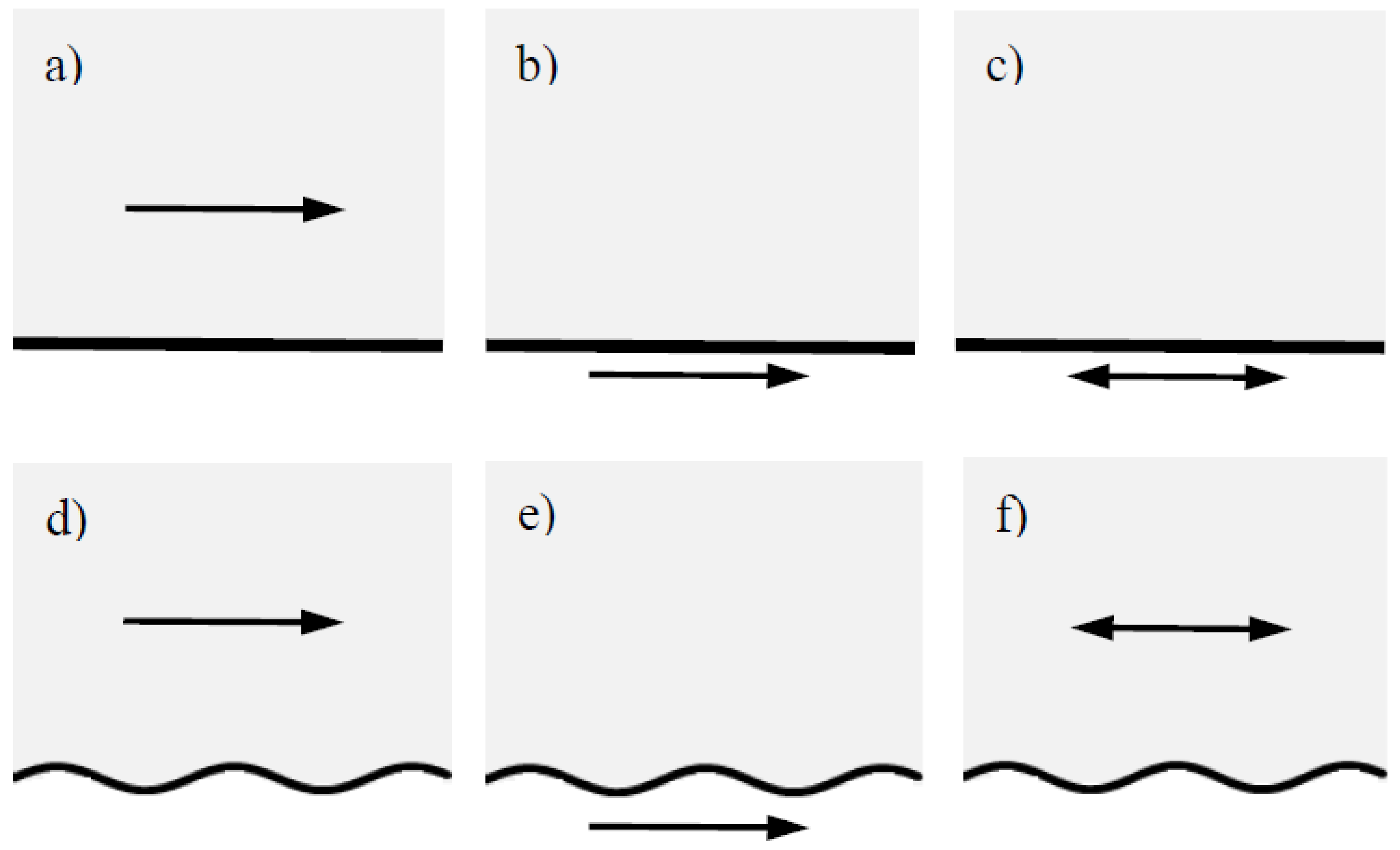
The oscillating flow over a wavy bottom problem has been approached by many authors due to its implication in sediment transport and ripple formation at the bottom of sea waves. In addition to the analytical approaches developed by Lyne [10], Kaneko and Honji [11], and Vittori [12], the works by Hara and Mei [21], Nishimura et al. [22], and Shen and Chan [23] can be mentioned. In all the above studies, the generatrix of the bed undulations is transverse to the direction of the main flow, as sketched in Figure 1.

The configuration in which the main flow is parallel to the bed deformation has also been studied, although all the literature found by the authors refers to the case in which the fluid is confined between two plates, and the flow is driven by a pressure gradient. Thus, Szumbarski [24] computed semi-analytically the velocity distribution and performed a linear stability analysis of the flow. Results of linear stability analysis have also been presented by Kowalewski et al. [25], Szumbarski and Błoński [26], and Moradi and Floryan [27]. Szumbarski et al. [28] studied numerically the effect of the wall corrugation on the hydraulic resistance of the flow. Among the results presented in their article, they show the circulation pattern induced by the velocity’s normal to the main flow direction, generating closed circulation cells. Gepner et al. [29] focused on the nonlinear solutions of the velocity field generated by the flow limited by two corrugated plates and the effect of the induced secondary currents enhancing diffusive transport. Yadav and Gepner [30] studied the effect on the flow instabilities for a geometry consisting in a fixed corrugated bottom plate and an upper moving plane plate. Later, Gepner and Floryan [31] approached numerically the flow driven by a pressure gradient of a fluid bounded by two sinusoidal walls which are in phase in flows at low and moderate sub-turbulent Reynolds numbers. As the fluid moves transverse to the plate deformations, it is prone to separation and generation of a recirculating region in the valleys of the walls. Previously, Smith [32] had studied the viscous Poiseuille 2-D flow, the walls of which had symmetrical and non-symmetrical cavities. His approach was theoretical, and the final equations were solved numerically. Bordner [33] had solved numerically the laminar boundary layer over a periodic stationary wavy surface, noticing the separation effect near the valleys of the wavy surface. A similar problem was solved by Sobey [6], who modeled and computed numerically the flow in an extracorporeal membrane oxygenator for both the steady and oscillatory flow conditions. Caponi et al. [34], also numerically, found that separation is obtained from the linearized Navier–Stokes equations for the laminar flow near a moving wavy surface. They also determined the range of validity of the linear approximation of the Navier–Stokes equations. Tsangaris and Leiter [35], using a perturbation method, and solving numerically some resulting equations, studied the separation of viscous laminar flows through wavy-walled channels. The separation characteristics of fluid flow inside two parallel wavy plates were also studied numerically by Mahmud et al. [36], who found that separation occurs for a critical Reynolds number which depends on dimensionless values of the amplitude and wavelength of the bed undulation.

Figure 1. Configuration analyzed in previous studies with free-surface or unconfined flows: (a) free-surface fluid flow over a fixed bottom [1]; (b) flow induced by the sudden motion of a plane plate [3]; (c) flow induced by the oscillatory motion of a plane plate [3]; (d) flow over a fixed wavy bed [4,5,9,13,14,15,16,17,18,19,20]; (e) flow resulting from the motion of a wavy bottom [9,34]; and (f) oscillatory flow over a wavy bottom [10,11,12,21,22,23].

Figure 1. Configuration analyzed in previous studies with free-surface or unconfined flows: (a) free-surface fluid flow over a fixed bottom [1]; (b) flow induced by the sudden motion of a plane plate [3]; (c) flow induced by the oscillatory motion of a plane plate [3]; (d) flow over a fixed wavy bed [4,5,9,13,14,15,16,17,18,19,20]; (e) flow resulting from the motion of a wavy bottom [9,34]; and (f) oscillatory flow over a wavy bottom [10,11,12,21,22,23].

So far, the cited references on flows over deformed walls correspond to pre-established geometries that do not change over time. However, there are studies in which the upper and lower walls confining the fluid fluctuate temporarily. Thus, Carlsson et al. [37,38] investigated a scenario involving the confinement of fluid within flexible walls, exhibiting transverse motion in the form of small amplitude standing waves. The velocity field was ascertained through a perturbation approach, revealing that streaming occurs at the second order, leading to the formation of cellular flow patterns in the channel. Lebbal et al. [39] analyzed the linear instabilities of the flow between flexible walls, considering that the base condition of the flow and the displacement of the walls are sinusoidal in both time and the direction of the main flow. The resulting equations were solved numerically. Vladimirov [40] considered that the flow domain is the half-space, with a boundary subject to tangential vibrations. The solution of the problem contains both oscillating and non-oscillating components and the streaming flows (either steady or unsteady) are obtained.

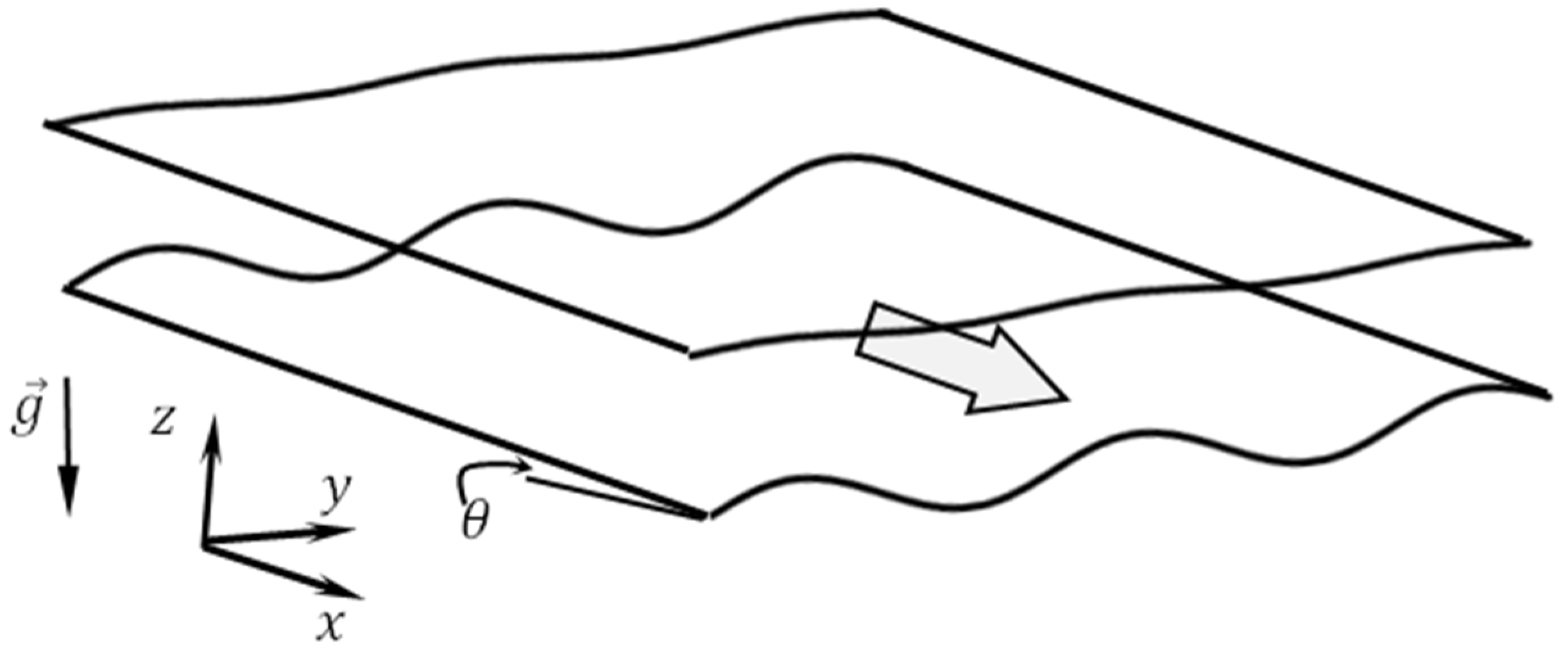
The goal of this article is to determine the velocity field of a free-surface flow when the bottom undergoes harmonic deformation in the direction transverse to the main flow (i.e., the undulations’ generatrix is parallel to the main flow), asymptotically approaching a maximum amplitude from a flat initial condition. The problem addressed here arose from the analysis of the generation of rills in their incipient stage due to overland flow over erodible soil [41]. The original problem is highly complex due to the interaction between the flow and the soil. As the soil erodes, it alters the geometry, subsequently changing the flow characteristics, and so on, until eventually reaching a final equilibrium condition. The primary objective of the article is not to solve the physical problem, as the equations accounting for soil erosion are not considered. The problem presented is merely an idealization of the bed deformation process, or a mimicry of it. Nevertheless, as far as the authors are aware, this has not been accomplished previously. Thus, the aim is to determine the flow characteristics of the rill formation process considering the depth of erosion to be small compared to the width of the rill. The main flow is assumed to be uniform (i.e., the flow depth does not change along the main flow direction), with the primary velocity component oriented in the direction transverse to the bed undulation (the main flow is parallel to the undulation generatrix), as illustrated in Figure 2. The specific goal of this paper is to present analytical solutions for the three velocity components and the distortion of the free surface caused by the deformation of the channel bottom. The bottom starts as initially flat and evolves to reach an equilibrium wavy shape.

2. Problem Formulation

The problem to be studied consists of determining the velocity field of the laminar flow with a free surface as it develops over a bottom inclined at an angle $\theta$ with respect to the horizontal in the main flow direction. The bottom features a small-amplitude undulation in the direction transverse to the flow that increases over time. A schematic of the problem and the coordinate system is presented in Figure 3. The flow extends indefinitely in the $x$ and $y$ directions. The origin of the $z$ axis is in the median plane that defines the bottom and is perpendicular to it. The $x$ axis is oriented in the direction of the main flow, forming an angle $\theta$ with the horizontal. The condition of small amplitude undulation is given by $a/h\ll 1$, where $a$ is the amplitude and $h$ the flow depth. Denoting by $\lambda$ the length of the undulation, the condition $a/\lambda \ll 1$ is also satisfied.

2.1. Governing Equations

The flow is governed by the continuity and Navier–Stokes equations [42], given below, where $\left(u,v,w\right)$ are the velocity components along $\left(x,y,z\right)$, $t$ is the time, $p$ is the fluid pressure, $g$ is the acceleration due to gravity, and $\rho$ and $\mu$ are the density and the viscosity of the fluid, respectively.

$$\frac{\partial u}{\partial x}+\frac{\partial v}{\partial y}+\frac{\partial w}{\partial z}=0$$

(1)

$$\rho \left(\frac{\partial u}{\partial t}+u\frac{\partial u}{\partial x}+v\frac{\partial u}{\partial y}+w\frac{\partial u}{\partial z}\right)=-\frac{\partial p}{\partial x}+\mu \left(\frac{{\partial }^{2}u}{\partial x^2}+\frac{{\partial }^{2}u}{\partial y^2}+\frac{{\partial }^{2}u}{\partial z^2}\right)+\rho g\sin \theta$$

(2)

$$\rho \left(\frac{\partial v}{\partial t}+u\frac{\partial v}{\partial x}+v\frac{\partial v}{\partial y}+w\frac{\partial v}{\partial z}\right)=-\frac{\partial p}{\partial y}+\mu \left(\frac{{\partial }^{2}v}{\partial x^2}+\frac{{\partial }^{2}v}{\partial y^2}+\frac{{\partial }^{2}v}{\partial z^2}\right)$$

(3)

$$\rho \left(\frac{\partial w}{\partial t}+u\frac{\partial w}{\partial x}+v\frac{\partial w}{\partial y}+w\frac{\partial w}{\partial z}\right)=-\frac{\partial p}{\partial z}+\mu \left(\frac{{\partial }^{2}w}{\partial x^2}+\frac{{\partial }^{2}w}{\partial y^2}+\frac{{\partial }^{2}w}{\partial z^2}\right)-\rho g\cos \theta$$

(4)

2.2. Boundary Conditions

On the bottom, the kinematic boundary condition, corresponding to no-slip, is applied to the components $u$ and $v$, while the bottom deformation rate is applied to $w$:

$$z=0, \forall \left(x,y,t\right) : u=v=0$$

(5)

$$\forall \eta \left(x,y,t\right) : w=\frac{d\eta }{dt}$$

(6)

where $\eta$ is the bottom level at $\left(x,y\right)$ for the time $t$, and it is a prescribed function.

In absence of capillarity $(a\ll \lambda )$ and wind effects, the dynamic boundary condition to be imposed at the free surface corresponds to a shear-free one:

$$z=h, \forall \left(x,y,t\right) : {\tau }_{xz}={\tau }_{yz}=0$$

(7)

To determine the free-surface deformation, the kinematic boundary condition is used:

$$z=h, \forall \left(x,y,t\right) : w=\frac{dh}{dt}$$

(8)

Thus, the system of differential Equations (1)–(4) with boundary conditions (5)–(8) allows us, formally, to solve the problem.

3. Solution

3.1. Transverse Velocity Field

The problem is solved by the perturbation method around a base flow [43,44]. The undisturbed condition (base flow) is denoted by the sub-index 0, and the perturbations are denoted by the sub-index 1. The base flow is defined by the velocity field $\left(u_0, 0, 0\right)$, such that the velocity vector is given by

$$\left(u,v,w\right)=\left(u_0+\epsilon u_1,\epsilon v_1, \epsilon w_1\right)$$

(9)

where $\epsilon =a/h_0$ is a small parameter and the velocity components $\left(u_1,v_1, w_1\right)$, properly scaled, are of order 1. In the same way, the flow depth $h$ is given by

$$h=h_0+\delta h_1$$

(10)

with $\delta \ll 1$ being a small parameter to be determined. The location $\eta$ of the bottom is chosen to be

$$\eta ={\eta }_R-x \sin \theta +a{f}_{\eta }{e}^{iky}$$

(11)

where ${\eta }_R$ is an arbitrary reference level, $a$ is the perturbation amplitude, $f_{\eta }$ is a function of time that describes the bottom deformation, $k=2\pi /\lambda$ is the wavenumber of the lateral bed deformation, and $i=\sqrt{-1}$. To simplify the algebra, Euler’s formula is used, understanding that the real part of the results must be taken.

Substituting the velocities given by Equation (9) in the system of Equations (1)–(4), the solution for the base flow is obtained:

$$\left(u_0,v_0, w_0\right)=\left(\frac{\rho g\sin \theta h_0^2}{\mu }\left(\frac{z}{h_0}-\frac{1}{2}\frac{z^2}{h_0^2}\right) , 0, 0\right)$$

(12)

$$p=\rho g\cos \theta \left(h_0-z\right)$$

(13)

Furthermore, by substituting the velocities provided by Equation (9) into the continuity and momentum equations (Equations (1)–(4)) and subsequently subtracting the equations pertaining to the base flow, we derive the equations governing the disturbances:

$$\frac{\partial v_1}{\partial y}+\frac{\partial w_1}{\partial z}=0$$

(14)

$$\frac{\partial u_1}{\partial t}+w_1\frac{\partial u_0}{\partial z}=\frac{\mu }{\rho }\left(\frac{{\partial }^2{u}_1}{\partial y^2}+\frac{{\partial }^2{u}_1}{\partial z^2}\right)$$

(15)

$$\frac{\partial v_1}{\partial t}=\frac{\mu }{\rho }\left(\frac{{\partial }^2{v}_1}{\partial y^2}+\frac{{\partial }^2{v}_1}{\partial z^2}\right)$$

(16)

$$\frac{\partial w_1}{\partial t}=\frac{\mu }{\rho }\left(\frac{{\partial }^2{w}_1}{\partial y^2}+\frac{{\partial }^2{w}_1}{\partial z^2}\right)$$

(17)

Note that, as the base flow is uniform and the bed is not perturbed along the $x$ direction, the continuity and momentum equations are independent of $x$. The velocity perturbations $v_1$ and $w_1$ satisfy the continuity equation in the plane $\left(y,z\right)$, so it is feasible to look for the solution in terms of a stream function ${\Psi }_1$:

$$\begin{array}{cc}{v}_1=\frac{\partial {\Psi }_1}{\partial z},& w_1=-\frac{\partial {\Psi }_1}{\partial y}\end{array}$$

(18)

Expressing Equations (16) or (17) in terms of the stream function, the solution for ${\Psi }_1$ is obtained. Using the momentum equation along $y$:

$$\frac{\partial }{\partial t}\left(\frac{\partial {\psi }_1}{\partial z}\right)=\frac{\mu }{\rho }\left(\frac{{\partial }^2}{\partial y^2}\left(\frac{\partial {\psi }_1}{\partial z}\right)+\frac{{\partial }^2}{\partial z^2}\left(\frac{\partial {\psi }_1}{\partial z}\right)\right)$$

(19)

The following structure for the solution of ${\psi }_1$ is proposed:

$${\psi }_1=f \Phi e^{iky}$$

(20)

where $f$ and $\Phi$ are functions of t and z, respectively, which must be determined. Substituting Equation (20) in Equation (19), the following ordinary differential equation for f is obtained:

$$\frac{\rho }{\mu }{e}^{iky}\frac{\partial f}{\partial t}\frac{\partial \Phi }{\partial z}=\left(-f{k}^2{e}^{iky}\frac{\partial \Phi }{\partial z}+f{e}^{iky}\frac{{\partial }^3\Phi }{\partial z^3}\right)$$

(21)

The above differential equation is of separable variables. Rearranging terms:

$$\frac{\rho }{\mu }\frac{1}{f}\frac{\partial f}{\partial t}=\frac{-k^2\frac{\partial \Phi }{\partial z}+\frac{{\partial }^3\Phi }{\partial z^3}}{\frac{\partial \Phi }{\partial z}}=\zeta$$

(22)

Thus, the temporal variation in the stream function is given by:

$$f={K_{1}e}^{\frac{\mu }{\rho }\zeta t}$$

(23)

The dependence of $\psi$ on $z$ is defined from the following differential equation:

$$\frac{{\partial }^3\Phi }{\partial z^3}-\left(\zeta +k^2\right)\frac{\partial \mathsf{\Phi }}{\partial z}=0$$

(24)

The $\zeta$ term of the above equations is not known and will be determined in the course of the solution. Although it can be a complex quantity, the final solution reveals that it is sufficient to perform the analysis assuming it is a real number. We will consider first that $\zeta$ is positive. Thus, the discriminant of $\omega =\sqrt{\zeta +k^2}$, is also positive and the solution of the above differential equation is

$$\Phi =A\sinh \left(\omega z\right)+B\cosh \left(\omega z\right)+C$$

(25)

with $A, B$, and $C$ as integration constants. Calling $\overline{A}=K_{1}A, \overline{B}=K_{1}B$, and $\overline{C}=K_{1}C$, after replacing Equations (23) and (25) in Equation (20), the stream function becomes:

$${\psi }_1=e^{\frac{\mu }{\rho }\zeta t}\left[\overline{A}\sinh \left(\omega z\right)+\overline{B}\cosh \left(\omega z\right)+\overline{C}\right]e^{iky}$$

(26)

Thus, the velocity components $v_1$ and $w_1$ are:

$$v_1=\omega e^{\frac{\mu }{\rho }\zeta t}\left[\overline{A}\cosh \left(\omega z\right)+\overline{B}\sinh \left(\omega z\right)\right]e^{iky}$$

(27)

$$w_1=-ik{e}^{\frac{\mu }{\rho }\zeta t}\left[\overline{A}\sinh \left(\omega z\right)+\overline{B}\cosh \left(\omega z\right)+\overline{C}\right]e^{iky}$$

(28)

The constants $\overline{A}, \overline{B},$ and $\overline{C}$ are determined from the boundary conditions, which correspond to two kinematic conditions at the bottom and one dynamic condition at the free surface. For $v_1$, the condition of no slip on the bottom is imposed. Since the deformation of the bed has been assumed to be small, the condition $v_1=0$ can be applied at $z=0$, from which Equation (27) yields $\overline{A}=0$. Thus:

$$v_1=\omega e^{\frac{\mu }{\rho }\zeta t}\overline{B}\sinh \left(\omega z\right)e^{iky}$$

(29)

$$w_1=-ik{e}^{\frac{\mu }{\rho }\zeta t}\left[\overline{B}\cosh \left(\omega z\right)+\overline{C}\right]e^{iky}$$

(30)

Applying the same argument of small deformation as for the bottom, the dynamic condition at the free-surface is applied at $z=h_0$, where the shear stress is zero. Replacing Equation (9) in the expression for the shear stress, it can be written as ${\tau }_{yz}={\tau }_{yz0}+\epsilon {\tau }_{yz1}$. With $v_1$ and $w_1$ from Equations (28) and (29), the shear stress associated with the perturbation is:

$${\tau }_{yz1}=\mu e^{\frac{\mu }{\rho }\zeta t}\left[\left({\omega }^2+k^2\right)\overline{B}\cosh \left(\omega z\right)+k^2\overline{C}\right]e^{iky}$$

(31)

The boundary condition ${\tau }_{yz1}=0$ at $z=h_0$ gives

$$\overline{B}=\frac{-k^2\overline{C}}{\left({\omega }^2+k^2\right)\cosh \left(\omega h_0\right)}$$

(32)

In this way, the stream function and transverse velocity components associated to the perturbation are given by:

$${\psi }_1=e^{\frac{\mu }{\rho }\zeta t}\overline{C}\left[\frac{\left({\omega }^2+k^2\right)\cosh \left(\omega h_0\right)-k^2\cosh \left(\omega z\right)}{\left({\omega }^2+k^2\right)\cosh \left(\omega h_0\right)}\right]e^{iky}$$

(33)

$$v_1=-\omega e^{\frac{\mu }{\rho }\zeta t}\overline{C}\left[\frac{k^2\sinh \left(\omega z\right)}{\left({\omega }^2+k^2\right)\cosh \left(\omega h_0\right)}\right]e^{iky}$$

(34)

$$w_1=-ik{e}^{\frac{\mu }{\rho }\zeta t}\overline{C}\left[\frac{\left({\omega }^2+k^2\right)\cosh \left(\omega h_0\right)-k^2\cosh \left(\omega z\right)}{\left({\omega }^2+k^2\right)\cosh \left(\omega h_0\right)}\right]e^{iky}$$

(35)

The second kinematic condition is enforced at the bottom ($z=0$). Its consideration, coupled with the temporal bottom deformation, facilitates the determination of the constants $\zeta$ and $\overline{C}$. In effect,

$${\left.w_1\right|}_{z=0}=\frac{d{\eta }_1}{dt}=\frac{\partial {\eta }_1}{\partial t}$$

(36)

Equation (11) can be written as $\eta ={\eta }_0+\epsilon {\eta }_1$, with ${\eta }_0={\eta }_R-x\sin \theta$ and ${\eta }_1$ given by:

$${\eta }_1=h_0{f}_{\eta }{e}^{iky}$$

(37)

where $f_{\eta }$ is a function of time. Given the structure imposed for the variation in time of the stream function $\left({\psi }_1 ~ e^{\frac{\mu }{\rho }\zeta t}\right)$, the deformation of the bed cannot be arbitrary. In particular, some of the forms that the function $f_{\eta }$ in Equation (37) can take are an exponential dependence on time, or a constant plus an exponential dependence. For this article, the following function is chosen, which characterizes bed deformation that increases from zero until reaching asymptotically a maximum equilibrium amplitude equal to $a$.

$$\begin{array}{ccc}{f}_{\eta }{=1-e}^{\beta t}& ,& \beta <0\end{array}$$

(38)

Thus,

$$\frac{\partial {\eta }_1}{\partial t}={-h}_0\beta e^{\beta t}{e}^{iky}$$

(39)

and the second kinematic condition is expressed as:

$$ik{e}^{\frac{\mu }{\rho }\zeta t}\overline{C}\left[\frac{\left({\omega }^2+k^2\right)\cosh \left(\omega h_0\right)-k^2}{\left({\omega }^2+k^2\right)\cosh \left(\omega h_0\right)}\right]=h_0\beta e^{\beta t}$$

(40)

To ensure the left side of Equation (40) is identical to the right side at any time, $\zeta$ and $\overline{C}$ must be:

$$\zeta =\beta \frac{\rho }{\mu }$$

(41)

$$\overline{C}=-i\frac{h_0\beta }{k}\left[\frac{\left({\omega }^2+k^2\right)\cosh \left(\omega h_0\right)}{\left({\omega }^2+k^2\right)\cosh \left(\omega h_0\right)-k^2}\right]$$

(42)

Thus, the stream function associated to $v_1$ and $w_1$ is:

$${\psi }_1=-i\frac{h_0\beta }{k}{e}^{\beta t}\left[\frac{\left({\omega }^2+k^2\right)\cosh \left(\omega h_0\right)-k^2\cosh \left(\omega z\right)}{\left({\omega }^2+k^2\right)\cosh \left(\omega h_0\right)-k^2}\right]e^{iky}$$

(43)

By construction, the stream function is composed of a base function (${\psi }_0$) and a disturbance, similar to velocities, shear stress, and bed deformation, i.e., $\psi {=\psi }_0+\epsilon {\psi }_1$. As the base transverse velocities are zero, the stream function results solely from the perturbations, so $\psi =\left(a/h_0\right){\psi }_1$. Thus, the stream function is given by:

$$\psi =-i\frac{a\beta }{k}{e}^{\beta t}\left[\frac{\left({\omega }^2+k^2\right)\cosh \left(\omega h_0\right)-k^2\cosh \left(\omega z\right)}{\left({\omega }^2+k^2\right)\cosh \left(\omega h_0\right)-k^2}\right]e^{iky}$$

(44)

From Equation (9), we have $v=\epsilon v_1$ and $w=\epsilon w_1.$ Introducing the expressions for the constants in Equations (34) and (35), the transverse velocities are obtained:

$$v=ia\beta e^{\beta t}\left[\frac{k\omega \sinh \left(\omega z\right)}{\left({\omega }^2+k^2\right)\cosh \left(\omega h_0\right)-k^2}\right]e^{iky}$$

(45)

$$w=-a\beta e^{\beta t}\left[\frac{\left({\omega }^2+k^2\right)\cosh \left(\omega h_0\right)-k^2\cosh \left(\omega z\right)}{\left({\omega }^2+k^2\right)\cosh \left(\omega h_0\right)-k^2}\right]e^{iky}$$

(46)

Taking the real part of Equations (44)–(46), the stream function and transverse velocities result to be:

$$\psi =\frac{a\beta }{k}{e}^{\beta t}\left[\frac{\left({\omega }^2+k^2\right)\cosh \left(\omega h_0\right)-k^2\cosh \left(\omega z\right)}{\left({\omega }^2+k^2\right)\cosh \left(\omega h_0\right)-k^2}\right]\sin \left(ky\right)$$

(47)

$$v=-a\beta e^{\beta t}\left[\frac{k\omega \sinh \left(\omega z\right)}{\left({\omega }^2+k^2\right)\cosh \left(\omega h_0\right)}\right]\sin \left(ky\right)$$

(48)

$$w=-a\beta e^{\beta t}\left[\frac{\left({\omega }^2+k^2\right)\cosh \left(\omega h_0\right)-k^2\cosh \left(\omega z\right)}{\left({\omega }^2+k^2\right)\cosh \left(\omega h_0\right)}\right]\cos \left(ky\right)$$

(49)

3.2. Deformation of the Free Surface

The deformation of the free surface is obtained from the kinematic condition at $z=h_0$:

$${\left.w\right|}_{z=h_0}=\frac{dh}{dt}=\frac{\partial h}{\partial t}$$

(50)

Using Equation (46), a differential equation for h results:

$$\frac{\partial h}{\partial t}=-a\beta e^{\beta t}\left[\frac{{\omega }^2\cosh \left(\omega h_0\right)}{\left({\omega }^2+k^2\right)\cosh \left(\omega h_0\right)-k^2}\right]e^{iky}$$

(51)

Performing the integration with the initial condition $t=0$, $h=h_0$, and taking the real part of the solution, the deformed free surface height is obtained.

$$h=h_0+a\left(1-e^{\beta t}\right)\left[\frac{{\omega }^2\cosh \left(\omega h_0\right)}{\left({\omega }^2+k^2\right)\cosh \left(\omega h_0\right)-k^2}\right]e^{iky}$$

(52)

Identifying terms in Equations (10) and (49), and taking the real part of ${\eta }_1$ (Equation (40)), the value of the amplitude of the free surface deformation $\delta$ is found:

$$\delta =\epsilon \left[\frac{{\omega }^2\cosh \left(\omega h_0\right)}{\left({\omega }^2+k^2\right)\cosh \left(\omega h_0\right)-k^2}\right]$$

(53)

Taking into account that $\omega h_0$ is always a finite quantity, it is easy to see that

$$0<\left[\frac{{\omega }^2\cosh \left(\omega h_0\right)}{\left({\omega }^2+k^2\right)\cosh \left(\omega h_0\right)-k^2}\right]<1$$

(54)

from which it results that the deformation of the free surface is always less than that of bottom. Moreover, based on the positive discriminant assumption of ω, it can be concluded from Equations (37) and (52) that both deformations are consistently in phase.

3.3. Longitudinal Velocity Distribution

Knowing the vertical perturbation of the component of the velocity along z (Equation (46)), and the solution at order 0 of $u$ (Equation (12)), the perturbation of $u$ can be obtained by integrating Equation (15), which becomes:

$$\begin{gathered} \frac{\partial u_1}{\partial t}-\frac{\rho g{h}_0^2\sin \theta }{\mu }\left(1-\frac{z}{h_0}\right)\beta e^{\beta t}{e}^{iky}\left(\frac{\left({\omega }^2+k^2\right)\cosh \left(\omega h_0\right)-k^2\cosh \left(\omega z\right)}{\left({\omega }^2+k^2\right)\cosh \left(\omega h_0\right)-k^2}\right) \\ =\frac{\mu }{\rho }\left(\frac{{\partial }^2{u}_1}{\partial y^2}+\frac{{\partial }^2{u}_1}{\partial z^2}\right) \end{gathered}$$

(55)

Consider that the solution $u_1$ has the following structure:

$$u_1=e^{\beta t}{e}^{iky}\left(\frac{\rho g{h}_0^2\sin \theta }{\mu }\right)U$$

(56)

where $U$ is a function of $z$. Replacing Equation (56) into Equation (55) and using the definitions of $\omega$ and $\zeta$, the equation for $u_1$ is reduced to:

$$\frac{d^{2}U}{d{z}^2}-{\omega }^{2}U+\left({\omega }^2-k^2\right)\left(1-\frac{z}{h_0}\right)\left(\frac{\left({\omega }^2+k^2\right)\cosh \left(\omega h_0\right)-k^2\cosh \left(\omega z\right)}{\left({\omega }^2+k^2\right)\cosh \left(\omega h_0\right)-k^2}\right)=0$$

(57)

The solution of Equation (57) is rather cumbersome. The following expression for $U$ results after imposing the boundary conditions of zero $x$-velocity at $z=0$ and no shear stress at $z=h_0$:

$$\begin{array}{cc}U=& \frac{A_1}{{\omega }^2}\left(1-\frac{z}{h_0}-\cosh \left(\omega z\right)\right)+\frac{B_1}{4{\omega }^2}\frac{z}{h_0}\cosh \left(\omega z\right)++\frac{B_1{h}_0}{2\omega }\left(\frac{z}{h_0}-\frac{1}{2}\frac{z^2}{h_0^2}\right)\sinh \left(\omega z\right)\\ & +[\frac{A_1}{{\omega }^2\cosh \left(\omega h_0\right)}\left(\frac{1}{\omega h_0}+\sinh \left(\omega h_0\right)\right)\\ & -\frac{B_1}{4{\omega }^2}\left(\frac{1}{\omega h_0}+\frac{\sinh \left(\omega h_0\right)}{\cosh \left(\omega h_0\right)}+\omega h_0\right)]\sinh \left(\omega z\right)\end{array}$$

(58)

Taking the real part of Equation (58) and adding the perturbation to the zeroth-order solution, the velocity along the x-axis is obtained ($u=u_0+\epsilon u_1$):

$$\begin{array}{cc}u=\frac{\rho g\sin \theta h_0^2}{\mu }& \{\left(\frac{z}{h_0}-\frac{z^2}{2{h_0}^2}\right)\\ & +\frac{a}{h_0}{e}^{\beta t}\cos \left(ky\right)\left(\frac{{\omega }^2-k^2}{{\omega }^2}\right)\{\left(\frac{\left({\omega }^2+k^2\right)\cosh \left(\omega h_0\right)}{\left({\omega }^2+k^2\right)\cosh \left(\omega h_0\right)-k^2}\right)\\ & \times \left(1-\frac{z}{h_0}-\cosh \left(\omega z\right)\right)\\ & +\frac{1}{4}\left(\frac{k^2}{\left({\omega }^2+k^2\right)\cosh \left(\omega h_0\right)-k^2}\right)\left(\frac{z}{h_0}\right)\cosh \left(\omega z\right)\\ & +\left(\frac{k^2}{\left({\omega }^2+k^2\right)\cosh \left(\omega h_0\right)-k^2}\right)\frac{h_0\omega }{2}\left(\frac{z}{h_0}-\frac{z^2}{2{h_0}^2}\right)\sinh \left(\omega z\right)\\ & +[\frac{1}{\cosh \left(\omega h_0\right)}\left(\frac{\left({\omega }^2+k^2\right)\cosh \left(\omega h_0\right)}{\left({\omega }^2+k^2\right)\cosh \left(\omega h_0\right)-k^2}\right)\left(\frac{1}{h_0\omega }+\sinh \left(\omega h_0\right)\right)\\ & -\frac{1}{4}\left(\frac{k^2}{\left({\omega }^2+k^2\right)\cosh \left(\omega h_0\right)-k^2}\right)\\ & \times \left(\frac{1}{h_0\omega }+\frac{\sinh \left(\omega h_0\right)}{\cosh \left(\omega h_0\right)}+h_0\omega \right)\left]\sinh \left(\omega z\right)\right\}\}\end{array}$$

(59)

Thus, the stream function (Equation (47)), the velocity field (Equations (48), (49) and (59)), and the free surface deformation (real part of Equation (52)) were determined for the case $\zeta +k^2>0$.

When $\zeta +k^2<0$, and $\omega$ is an imaginary number, there is a slight change in the solutions. From the definition of $\omega$, another variable $\varpi$ is introduced such that ${\varpi }^2=$ $-\left(\zeta +k^2\right)>0$. Thus $\omega =i\varpi$, and the expressions for the stream function, velocities, and free surface are:

$$\psi =\frac{a\beta }{k}{e}^{\beta t}\left[\frac{\left({\varpi }^2-k^2\right)\cos \left(\varpi h_0\right)+k^2\cos \left(\varpi z\right)}{\left({\varpi }^2-k^2\right)\cos \left({\varpi h}_0\right)+k^2}\right]\sin \left(ky\right)$$

(60)

$$v=-a\beta e^{\beta t}\left[\frac{k\varpi \sin \left(\varpi z\right)}{\left({\varpi }^2-k^2\right)\cos \left({\varpi h}_0\right)+k^2}\right]\sin \left(ky\right)$$

(61)

$$w=-a\beta e^{\beta t}\left[\frac{\left({\varpi }^2-k^2\right)\cos \left(\varpi h_0\right)+k^2\cos \left(\varpi z\right)}{\left({\varpi }^2-k^2\right)\cos \left({\varpi h}_0\right)+k^2}\right]\cos \left(ky\right)$$

(62)

$$h=h_0+a\left(1-e^{\beta t}\right)\left[\frac{{\varpi }^2\cos \left(\varpi h_0\right)}{\left({\varpi }^2-k^2\right)\cos \left(\varpi h_0\right)+k^2}\right]\cos \left(ky\right)$$

(63)

$$\begin{array}{cc}u=\frac{\rho g\sin \theta h_0^2}{\mu }& \{\left(\frac{z}{h_0}-\frac{z^2}{2{h_0}^2}\right)\\ & +\frac{a}{h_0}{e}^{\beta t}\cos \left(ky\right)\left(\frac{{\varpi }^2+k^2}{{\varpi }^2}\right)\{\left(\frac{\left({\varpi }^2-k^2\right)\cos \left(\varpi h_0\right)}{\left({\varpi }^2-k^2\right)\cos \left(\varpi h_0\right)+k^2}\right)\\ & \times \left(1-\frac{z}{h_0}-\cos \left(\varpi z\right)\right)-\frac{1}{4}\left(\frac{k^2}{\left({\varpi }^2-k^2\right)\cos \left(\varpi h_0\right)+k^2}\right)\left(\frac{z}{h_0}\right)\cos \left(\varpi z\right)\\ & +\left(\frac{k^2}{\left({\varpi }^2-k^2\right)\cos \left(\varpi h_0\right)+k^2}\right)\frac{h_0\varpi }{2}\left(\frac{z}{h_0}-\frac{z^2}{2{h_0}^2}\right)\sin \left(\varpi z\right)\\ & +[\left(\frac{\left({\varpi }^2-k^2\right)}{\left({\varpi }^2-k^2\right)\cos \left(\varpi h_0\right)+k^2}\right)\left(\frac{1}{h_0\varpi }-\sin \left(\varpi h_0\right)\right)\\ & -\frac{1}{4}\left(\frac{k^2}{\left({\varpi }^2-k^2\right)\cos \left(\varpi h_0\right)+k^2}\right)\\ & \times \left(-\frac{1}{h_0\varpi }+\frac{\sin \left(\varpi h_0\right)}{\cos \left(\varpi h_0\right)}+h_0\varpi \right)\left]\sin \left(\varpi z\right)\right\}\}\end{array}$$

(64)

The ratio between the amplitude of the free surface and the amplitude of the deformation of the bottom for ${\omega }^2<0$ is given by

$$\frac{\delta }{\epsilon }=\left[\frac{{\varpi }^2\cos \left(\varpi h_0\right)}{\left({\varpi }^2-k^2\right)\cos \left(\varpi h_0\right)+k^2}\right]$$

(65)

4. Analysis and Visualization of the Solution

4.1. Dimensionless Parameters

To generalize the results, $h_0$, $\lambda$, and $\beta$ are used as scales to make dimensionless $z, y$, and $t$, respectively:

$$z^{\ast }=\frac{z}{h_0},\hspace{1em}{y}^{\ast }=\frac{y}{\lambda },\hspace{1em}{t}^{\ast }=-\beta t$$

(66)

The minus sign in $t^{\ast }$ appears because $\beta <0$ (Equation (38)). The dimensionless bed perturbation (Equations (37) and (38)) is written as ${\eta }_1^{\ast }=\left(1-e^{-t^{\ast }}\right)e^{i{y}^{\ast }}$. $\widehat{k}=1/\lambda$ is also defined, such that ${\widehat{k}}^{\ast }=\lambda \widehat{k}=1$. Thus, the following dimensionless parameters arise:

$$B=-\frac{\beta \rho {\lambda }^2}{\mu },\hspace{1em}\Omega =\omega \lambda =\sqrt{1-B}, \Lambda =\frac{h_0}{\lambda }$$

(67)

$B$ is always positive and it appears naturally from the scaling of the equations for the perturbed components of the transverse velocities $v_1$ or $w_1$ (Equations (16) or (17)). Let $\mathcal{V}$ be a scale for the velocity $v_1$ such that the dimensionless velocity is given by ${\widehat{v}}_1=v_1/\mathcal{V}$. In terms of the dimensionless variables, Equation (16) becomes:

$$-\beta \mathcal{V}\frac{\partial {\widehat{v}}_1}{\partial t^{\ast }}=\frac{\mu }{\rho }\left(\frac{\mathcal{V}}{{\lambda }^2}\frac{{\partial }^2{\widehat{v}}_1}{\partial y^{\ast 2}}+\frac{\mathcal{V}}{h_0^2}\frac{{\partial }^2{\widehat{v}}_1}{\partial z^{\ast 2}}\right)$$

(68)

$$-\beta \frac{\partial {\widehat{v}}_1}{\partial t^{\ast }}=\frac{\mu }{\rho {\lambda }^2}\left(\frac{{\partial }^2{\widehat{v}}_1}{\partial y^{\ast 2}}+{\left(\frac{\lambda }{h_0}\right)}^2\frac{{\partial }^2{\widehat{v}}_1}{\partial z^{\ast 2}}\right)$$

(69)

$$B\frac{\partial {\widehat{v}}_1}{\partial t^{\ast }}=\left(\frac{{\partial }^2{\widehat{v}}_1}{\partial y^{\ast 2}}+\frac{1}{{\Lambda }^2}\frac{{\partial }^2{\widehat{v}}_1}{\partial z^{\ast 2}}\right)$$

(70)

Calling $\mathcal{W}$ the velocity scale to make dimensionless the perturbation of the velocity in the z direction, ${\widehat{w}}_1=w_1/\mathcal{W}$. Thus, the dimensionless version of Equation (17) is:

$$B\frac{\partial {\widehat{w}}_1}{\partial t^{\ast }}=\left(\frac{{\partial }^2{\widehat{w}}_1}{\partial y^{\ast 2}}+\frac{1}{{\Lambda }^2}\frac{{\partial }^2{\widehat{w}}_1}{\partial z^{\ast 2}}\right)$$

(71)

As the momentum equations for disturbances in the $y$ and $z$ directions are linear and depend on only one velocity component, the final result is independent of the chosen velocity scale, depending on two parameters, $B$ and $\Lambda$. From the above equations, clearly $B$ is a kind of Reynolds number that represents the ratio between the fluid’s inertia due to the vertical deformation of the bed and the fluid’s viscous resistance. Note that from the continuity equation for the perturbed velocity components (Equation (14)), the following relationship between the velocity scales is obtained: $\mathcal{V}/\mathcal{W}~\lambda /h_0={\Lambda }^{-1}$.

For $0\le B\le 1$, $\Omega$ is a real number, with $0\le \Omega \le 1$, and the solutions for the stream function, velocity field, flow depth, and free surface deformation involve hyperbolic functions (Equations (47)–(49), (52), (53), and (59)). When $B>1$, $\Omega$ is an imaginary number and the hyperbolic functions become trigonometric ones (Equations (60)–(65)), changing the behavior of the solutions, as will be seen below. Defining $\tilde{\Omega }=\sqrt{B-1}>0$, $=\tilde{\Omega }i$ and $\tilde{\Omega }=\mathcal{\omega }\lambda$.

4.1.1. Behavior of the Solutions When $0\le B\le 1$ ($\Omega$ Real)

Taking the real part of Equation (44) and rendering it dimensionless results in:

$${\psi }^{\ast }=\frac{\psi }{a\beta }=e^{-t^{\ast }}\left[\frac{\left({\Omega }^2+1\right)\cosh (\Lambda \Omega )-\cosh (\Lambda \Omega z^{\ast })}{\left({\Omega }^2+1\right)\cosh \left(\Lambda \Omega \right)-1}\right]\sin \left(y^{\ast }\right)$$

(72)

Similarly, we can define $v^{\ast }$ and $w^{\ast }$ as new dimensionless velocity components, such that

$$v^{\ast }=\frac{v}{-a\beta }=e^{-t^{\ast }}\left[\frac{\Omega \sinh (\mathsf{\Lambda }\Omega z^{\ast })}{\left({\Omega }^2+1\right)\cosh \left(\mathsf{\Lambda }\Omega \right)-1}\right]\sin \left(y^{\ast }\right)$$

(73)

$$w^{\ast }=\frac{w}{-a\beta }=e^{-t^{\ast }}\left[\frac{\left({\Omega }^2+1\right)\cosh (\Lambda \Omega )-\cosh (\Lambda \Omega z^{\ast })}{\left({\Omega }^2+1\right)\cosh (\Lambda \Omega )-1}\right]\cos \left(y^{\ast }\right)$$

(74)

The transverse velocities have been scaled with $-\alpha \beta$ and not with the scales $\mathcal{V}$ and $\mathcal{W}$, solely to facilitate the graphical presentation of the results. Indeed, by having the product $-\alpha \beta$ appear as a coefficient in the transverse velocities, generating the new variables $v^{\ast }$ and $w^{\ast }$ reduces the number of parameters to be considered.

Denoting $A=\delta /\epsilon$ as the ratio between the deformation of the free surface and the bed, Equation (53) in terms of the dimensionless parameters is

$$A=\frac{\epsilon h_1^{\ast }}{\epsilon {\eta }_1^{\ast }}=\left[\frac{{\Omega }^2\cosh (\Lambda \Omega )}{\left({\Omega }^2+1\right)\cosh (\Lambda \Omega )-1} \right]$$

(75)

For $0\le B\le 1$ (i.e., $0\le \Omega \le 1$), $A$ is in the range $0\le A\le 1$ for any value of $\Lambda \ge 0$. This means that the amplitude of the free surface deformation is always smaller than the bed deformation. Also, the term in brackets in Equations (73) and (74) is always less than 1, for any $z^{\ast }\le 1$.

Finally, the dimensionless perturbation of the longitudinal component of the velocity is as follows:

$$\begin{array}{cc}{u}_1^{\ast }& =\frac{u_1}{\rho g\sin \theta h_0^2/\mu }\\ & =e^{-t^{\ast }}\cos \left(y^{\ast }\right)\left(\frac{{\Omega }^2-1}{{\Omega }^2}\right)\{\left(\frac{\left({\Omega }^2+1\right)\cosh \left(\Lambda \Omega \right)}{\left({\Omega }^2+1\right)\cosh \left(\Lambda \Omega \right)-1}\right)\\ & \times \left(1-z^{\ast }-\cosh (\Lambda \Omega z^{\ast })\right)\\ & +\frac{1}{4}\left(\frac{1}{\left({\Omega }^2+1\right)\cosh \left(\Lambda \Omega \right)-1}\right)z^{\ast }\cosh (\Lambda \Omega z^{\ast })\\ & +\left(\frac{1}{\left({\Omega }^2+1\right)\cosh \left(\Lambda \Omega \right)-1}\right)\frac{1}{2}\Lambda \Omega \left(z^{\ast }-\frac{1}{2}{z^{\ast }}^2\right)\sinh (\Lambda \Omega z^{\ast })\\ & +[\frac{1}{\cosh (\Lambda \Omega )}\left(\frac{\left({\Omega }^2+1\right)\cosh \left(\Lambda \Omega \right)}{\left({\Omega }^2+1\right)\cosh \left(\Lambda \Omega \right)-1}\right)\left(\frac{1}{\Lambda \Omega }+\sinh \left(\Lambda \Omega \right)\right)\\ & -\frac{1}{4}\left(\frac{1}{\left({\Omega }^2+1\right)\cosh \left(\Lambda \Omega \right)-1}\right)\\ & \times \left(\frac{1}{\Lambda \Omega }+\frac{\sinh \left(\Lambda \Omega \right)}{\cosh (\Lambda \Omega )}+\Lambda \Omega \right)\left]\sinh (\Lambda \Omega z^{\ast })\right\}\end{array}$$

(76)

It is easier to realize the analytical results presented above if they are plotted as in Figure 4, Figure 5, Figure 6, Figure 7 and Figure 8. It must be noted that the general behavior of the streamlines, velocity components, and deformation of the free surface essentially does not change with the values of $\Omega$ and $\Lambda$, and the general shapes are those presented in the figures. Arbitrary values of these parameters were used in the computations. The spanwise dimension ($y$-axis) of the plots correspond to a wavelength $\lambda$ of the bed deformation. The obtained results require small values of $\epsilon$ to maintain the validity of the linear approximation. However, using $\epsilon <0.1$ produces results with variations that are practically imperceptible in the graphs. Thus, to facilitate visualizing the variations introduced by the first-order term in the base solution, the amplitudes of the perturbations were greatly amplified in the figures depicting flow properties.

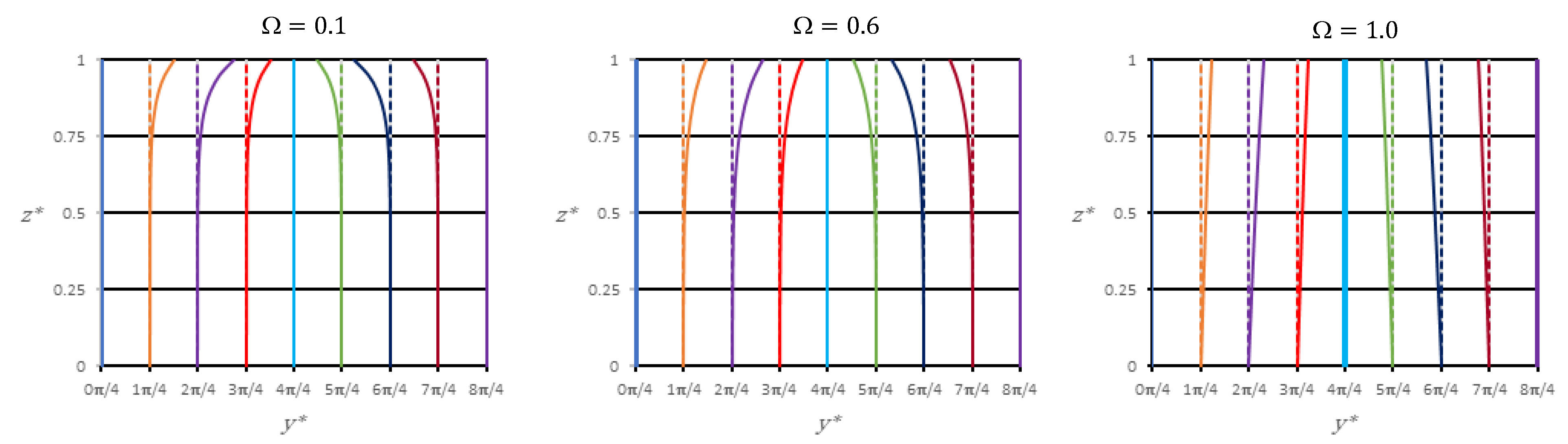
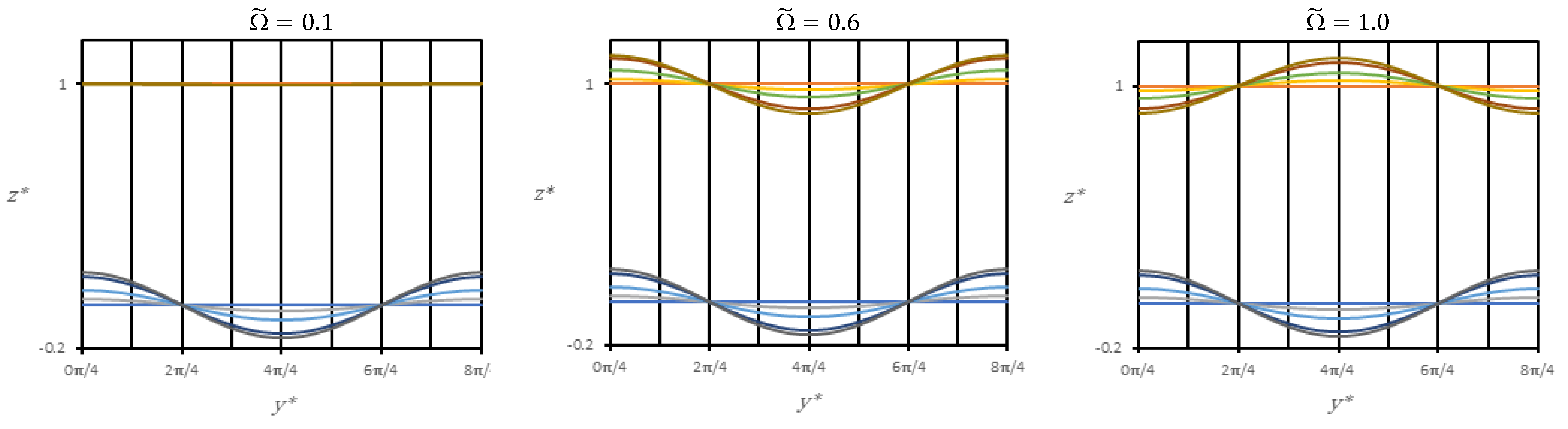
4.1.2. Behavior of the Solutions When $B\ge 1$ ($\Omega$ Imaginary)

By employing relationships that transform hyperbolic functions of a complex variable into trigonometric ones and taking their real parts, we obtain the dimensionless versions of the equations for the streamline, velocity components, perturbed deformation of the free surface, and the ratio between the deformation of the free surface and the bed. They are presented below:

$${\psi }^{*}=\frac{\psi }{a\beta }=e^{-t^{*}}\left[\frac{\left(1-{\tilde{\Omega }}^2\right)\cos \left(\Lambda \tilde{\Omega }\right)-\cos \left(\Lambda \tilde{\Omega }{z}^{\ast }\right)}{\left(1-{\tilde{\Omega }}^2\right)\cos \left(\Lambda \tilde{\Omega }\right)-1}\right]\sin \left(y^{\ast }\right)$$

(77)

$$v^{\ast }=\frac{v}{-a\beta }=-e^{-t^{\ast }}\left[\frac{\tilde{\Omega }\sin \left(\Lambda \tilde{\Omega }{z}^{\ast }\right)}{\left(1-{\tilde{\Omega }}^2\right)\cos \left(\Lambda \tilde{\Omega }\right)-1}\right]\sin \left(y^{\ast }\right)$$

(78)

$$w^{\ast }=\frac{w}{-a\beta }=e^{-t^{\ast }}\left[\frac{\left(1-{\tilde{\Omega }}^2\right)\cos \left(\Lambda \tilde{\Omega }\right)-\cos \left(\Lambda \tilde{\Omega }{z}^{\ast }\right)}{\left(1-{\tilde{\Omega }}^2\right)\cos \left(\Lambda \tilde{\Omega }\right)-1}\right]\cos \left(y^{\ast }\right)$$

(79)

$$\epsilon h_1^{\ast }=\epsilon \left(1-e^{-t^{\ast }}\right)\cos \left(y^{\ast }\right)\left[\frac{-{\tilde{\Omega }}^2\cos \left(\Lambda \tilde{\Omega }\right)}{\left(1-{\tilde{\Omega }}^2\right)\cos \left(\Lambda \tilde{\Omega }\right)-1} \right]$$

(80)

$$A=\frac{\epsilon h_1^{\ast }}{\epsilon {\eta }_1^{\ast }}=\left[\frac{-{\tilde{\Omega }}^2\cos \left(\Lambda \tilde{\Omega }\right)}{\left(1-{\tilde{\Omega }}^2\right)\cos \left(\Lambda \tilde{\Omega }\right)-1} \right]$$

(81)

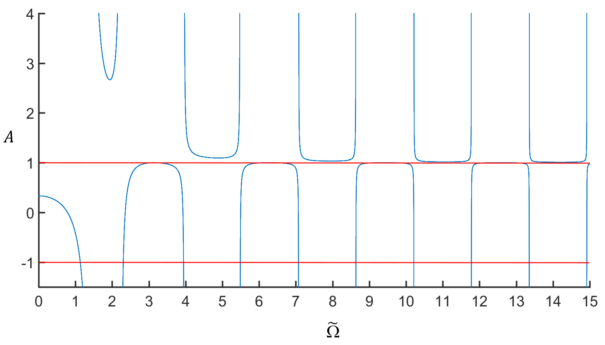
It is worth discussing the behavior of $A$ before analyzing the stream function, velocities, and free surface deformation. $A$ becomes indeterminate when $\left(1-{\tilde{\Omega }}^2\right)\cos \left(\Lambda \tilde{\Omega }\right)-1=0$, fluctuating between positive and negative values, as it is observed in Figure 9. Although the figure corresponds to the particular case $\Lambda =2$, the general behavior is the same for any $\Lambda$. The change in sign of $A$ indicates that the free surface deformation is not always in phase with the bed deformation. Furthermore, due to viscous dissipation, it is not possible to have values of the amplitude of the free surface greater than the amplitude of the bed, limiting the range of $A$ to the interval $-1<A<1$. This last condition is important because it imposes a relation between $\Lambda$ and $\tilde{\Omega }$. For the upper limit $A=1$, $\Lambda \tilde{\Omega }=2\pi n$ with $n=\mathrm{0,1},2, \dots$ must be satisfied. For the lower limit $A=-1$, the relationship between $\Lambda$ and $\tilde{\Omega }$ is given by $\left(2{\tilde{\Omega }}^2-1\right)\cos \left(\tilde{\Omega }\right)=1$. For a given interval of $\tilde{\Omega }$, the larger the value of $\Lambda$, the greater the number of branches of $A$.

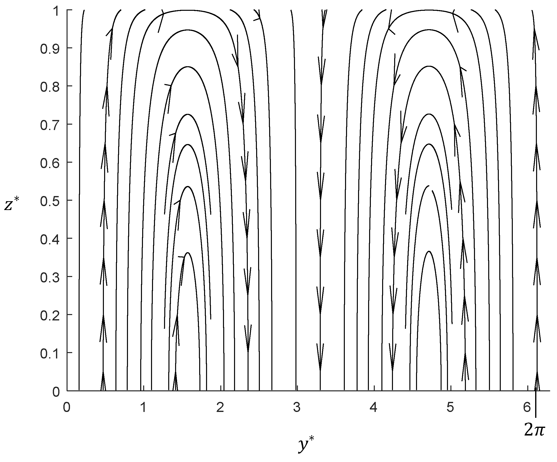
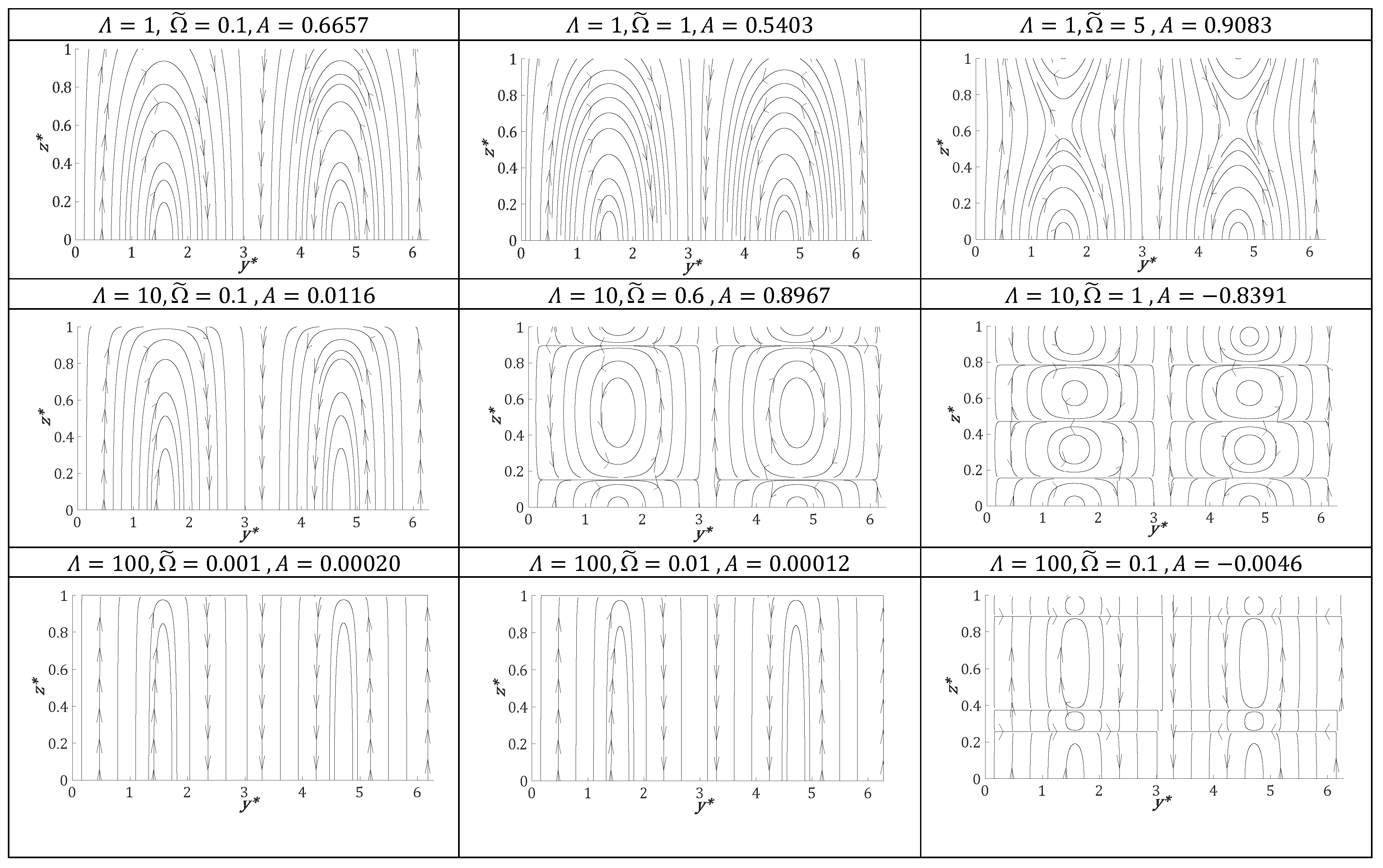
The behavior of ${\psi }^{\ast }$ when $\Omega$ is imaginary is completely different from the case when it is real. The presence of an oscillatory function like cosine could lead to a change in the sign of ${\psi }^{\ast }$ along $z^{\ast }$ for a given transversal location $y^{\ast }$. In contrast to the case of real $\Omega$, many configurations of streamlines arise depending on the values of $\Lambda$ and $\tilde{\Omega }$, as shown in the examples in Figure 10. This sometimes generates cells to make compatible the velocities induced simultaneously by both bottom and free surface deformations.

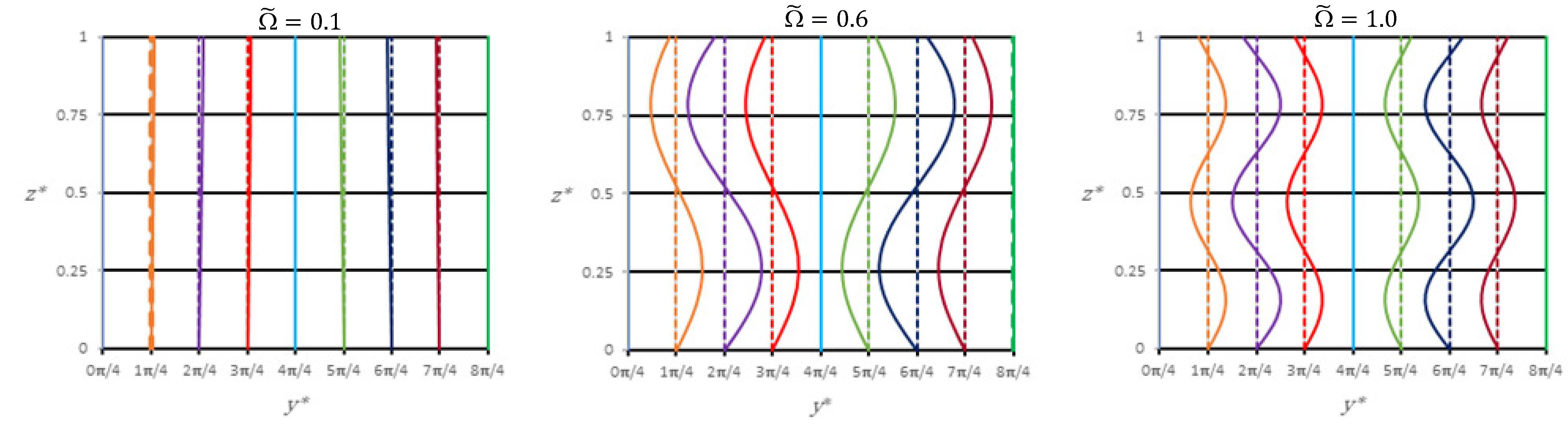
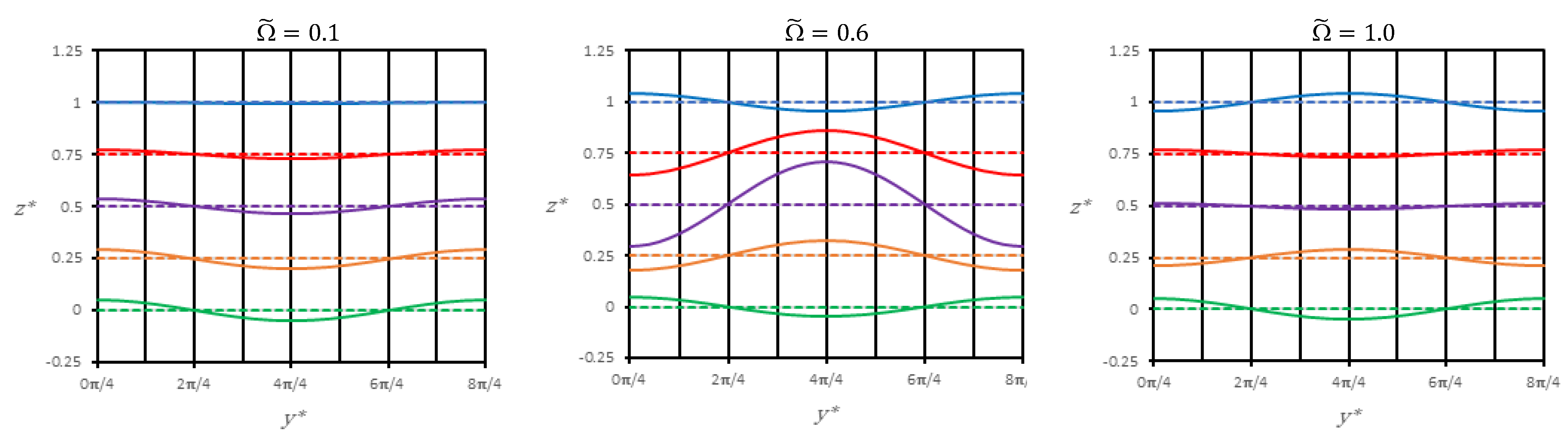
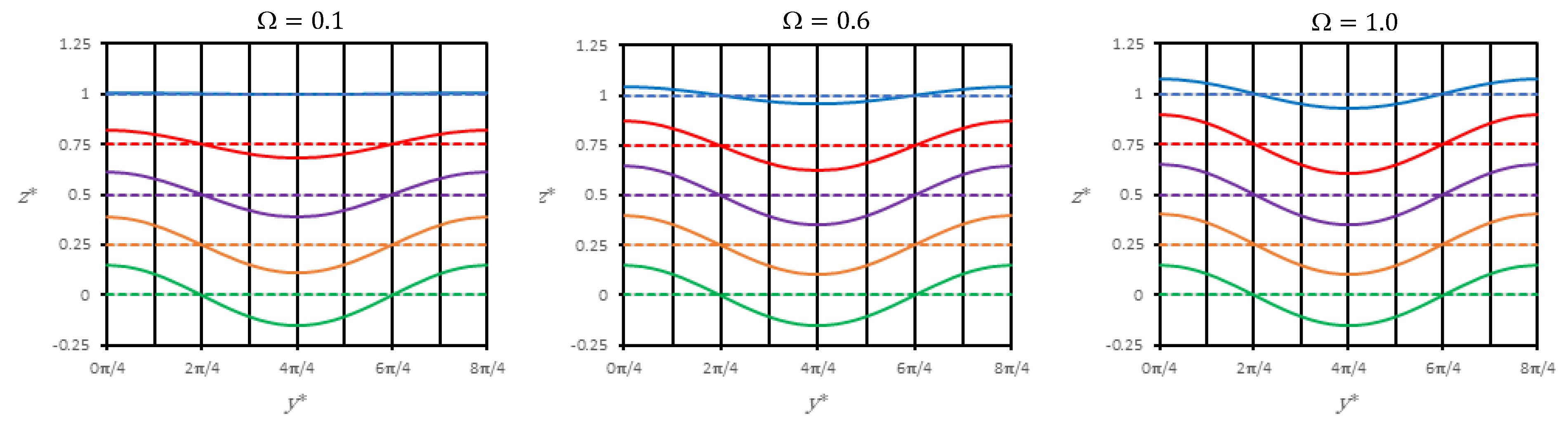
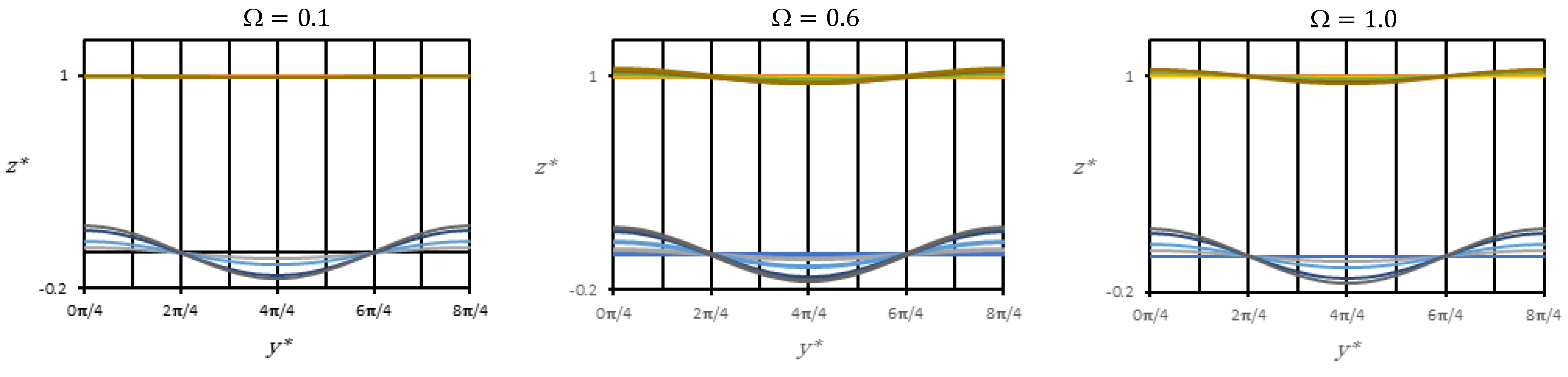
The dimensionless transverse velocities $v^{\ast }$ and $w^{\ast }$ are presented in Figure 11 and Figure 12, respectively, for the three values of $\tilde{\Omega }$ corresponding to $\Lambda =10$ shown in Figure 10. The change in sign of the velocities is a result of the presence of circulation cells. The deformations of the free surface and bottom over time for $\Lambda =10$ are shown in Figure 13. 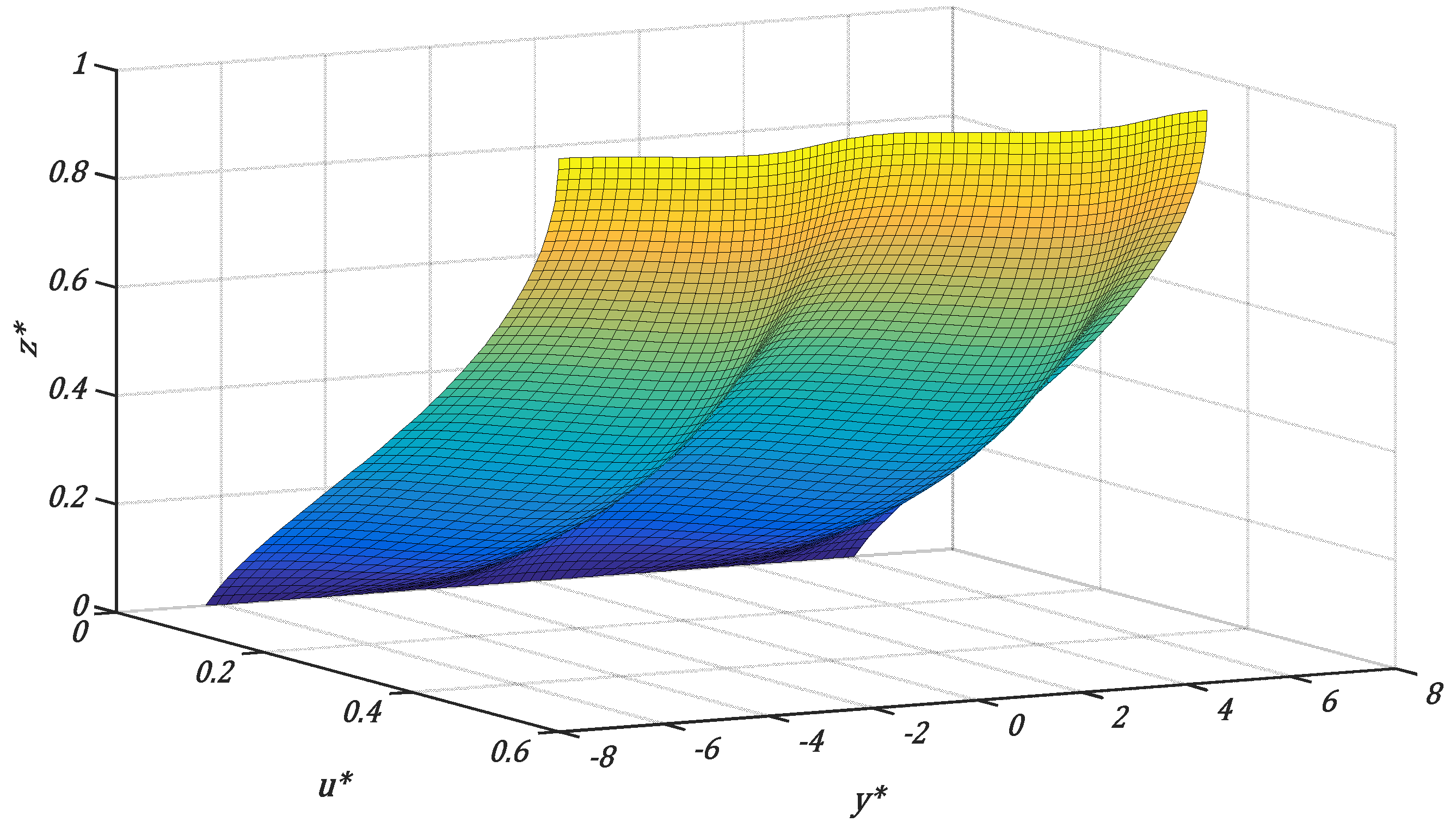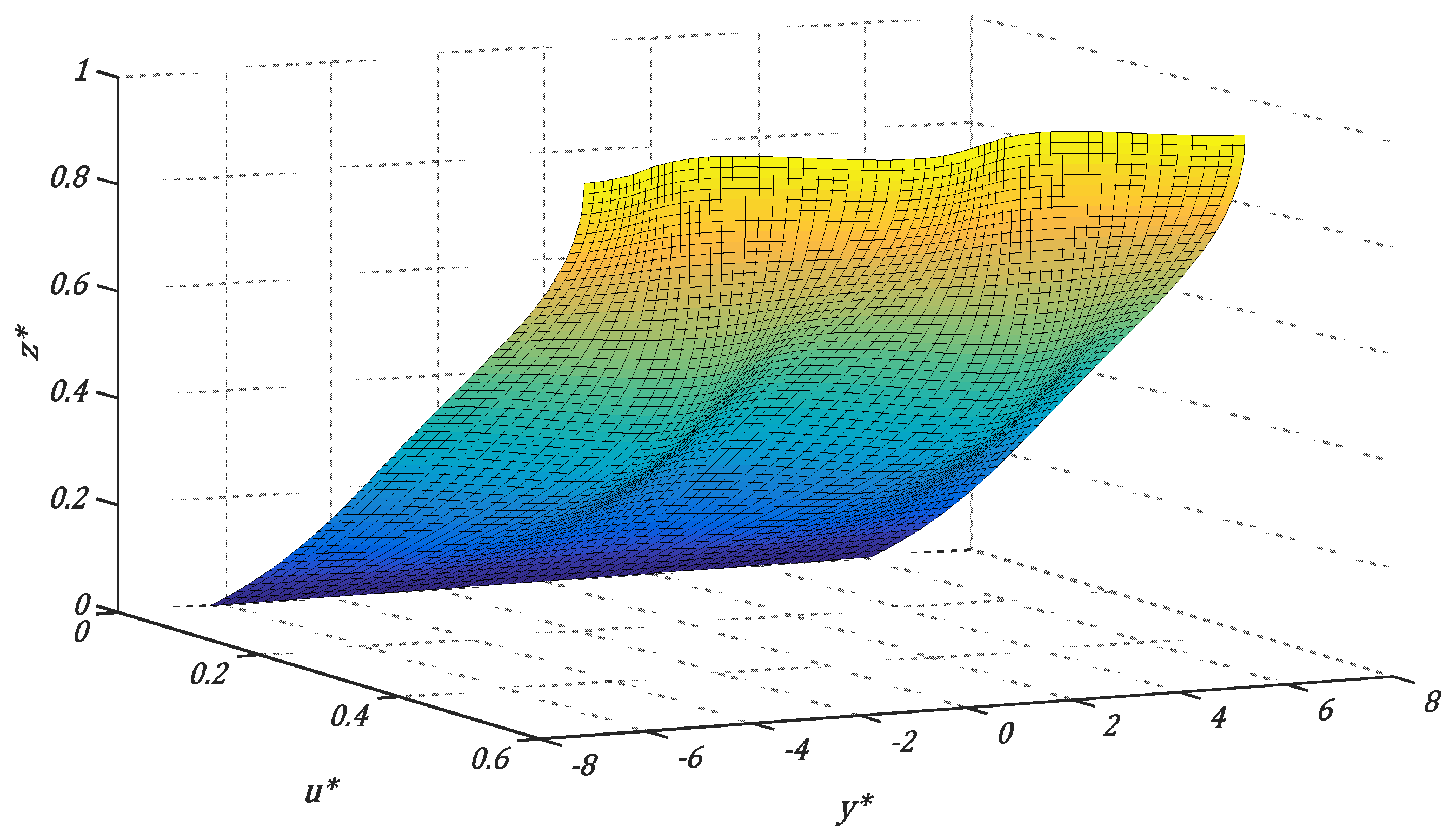As it was indicated, both deformations can be in phase or out of phase by $\pi$, depending on the value of $\tilde{\Omega }$ ($A$ can be positive or negative). Finally, the dimensionless main flow velocity $u^{\ast }$ is presented in Figure 14, where the effect of the perturbation on the base velocity has been exaggerated for easier visualization.

4.2. Flow Separation

The presence of a flow over protrusions on the channel bed may lead to flow separation. Currently, there is a lack of studies determining the separation conditions for the specific configuration explored in this article—convergent flows over a sinusoidally undulated bed with a free surface. Nevertheless, as an initial approximation, extrapolating results from studies on pressure-driven flows in two-dimensional pipes with sinusoidally varying walls along the main flow direction is feasible. To estimate the separation condition for transverse flow with a free surface, we rely on a previous result obtained for flows constrained by wavy walls. This estimation is made despite differences in flow configurations, such as the constant net flow existing in the $x$-direction in pressure-driven cases (where separation occurs in the $xz$ plane), which contrasts with the variable cross-sectional flow ($yz$ plane) of the problem addressed in this article.

In this regard, the analytical results of Tsangaris and Leiter [35] based on the separation of flow from a laminar boundary layer over a sinusoidally varying surface is applied. These authors determined that the separation is conditioned by a critical Reynolds number ($R{e}_c$) that is related to the dimensionless amplitude of bed deformation ($\epsilon$). In general, this relationship is not simple and must be determined by numerically integrating the vorticity equation in terms of the stream function, obtaining a relationship $R{e}_c=\phi \left(\epsilon \right)$, which they graphically present in their article. The critical Reynolds number at which separation occurs is defined as $R{e}_c=Ub/\nu$, where $b$ is half of the mean separation between walls, and $U$ is the average velocity. $\epsilon =a/b$, with $a$ being the amplitude of the wall deformation. For large Reynolds numbers, the authors provide the approximation $\phi \approx 7.563/\epsilon ^2$.

To apply the separation point condition of Tsangaris and Leiter to the cases generated in our study, the velocity $U$ is taken as the maximum transverse velocity $v_{max}$, and $b$ is set equal to the flow height coordinate, $z_{max}$. Thus, the critical Reynolds number is given by ${Re}_c=\rho v_{max}{z}_{max}/\mu$, which, expressed in terms of the dimensionless variables given by Equations (66) and (67), is written as $R{e}_c=\epsilon B{\Lambda }^2{v}_{max}^{\ast }{z}_{Vmax}^{\ast }$. For $0<B \le 1$ and considering the most unfavorable scenario ($\left|\sin \left(y^{\ast }\right)\right|\le 1 , z_{max}^{\ast }=1 , e^{-t^{\ast }}\le 1),$ an upper bound for ${Re}_c$ is obtained:

$${Re}_c<{\epsilon }^2\left(1-{\Omega }^2\right){\Lambda }^2\left|\frac{\Omega \sinh (\Lambda \Omega )}{\left({\Omega }^2+1\right)\cosh \left(\Lambda \Omega \right)-1}\right|<\phi \left(\epsilon \right)$$

(82)

Similarly, for the case $B>1$, the flow separation condition is bounded by

$$R{e}_c<{\epsilon }^2\left(1+{\tilde{\Omega }}^2\right){\Lambda }^2\left|\frac{\tilde{\Omega }}{\left(1-{\tilde{\Omega }}^2\right)\cos \left(\Lambda \tilde{\Omega }\right)-1}\right|<\phi \left(\epsilon \right)$$

(83)

As an example, for the case $0<B\le 1$, if $\epsilon =0.1, \Lambda =10$, and $\Omega =0.6$, the result is ${Re}_c<0.2$. Similarly, when $B>1$, considering $\epsilon =0.1, \Lambda =100$, and $\tilde{\Omega }\approx 0.1$, the result is ${Re}_c$ < 5.5. In both cases, the values of ${Re}_c$ are much lower than $\phi \left(\epsilon \right)$, obtained from the graphical relationship presented in the article by Tsangaris and Leiter [35].

Choosing $\epsilon =0.1$ represents merely an arbitrary value for the dimensionless amplitude of the bed deformation ($\epsilon =a/h_0$). While the preceding results confirm the absence of flow separation, they do not guarantee the extent to which the linear solution deviates from the one obtained by accounting for the non-linear terms in the momentum equations. In strict terms, linearizing the problem requires $\epsilon \ll 1$. Therefore, it is reasonable to expect that the results obtained from the linear approach are valid for $\epsilon <0.01$. However, this a priori assumption needs validation through a nonlinear analytical solution of the problem or via numerical modeling. Both approaches are beyond the scope of this work, and the authors are not aware of this problem being addressed previously.

4.3. Conditions for the Validity of the Results Obtained from the Linearized Equations

In order to determine the limitations of the applicability of the first-order results obtained in this article, the conditions that the parameters must satisfy when non-dimensionalizing the linearized equations are established below. The analysis can be carried out interchangeably for the momentum equations of perturbations in the $y$ or $z$ directions, taking into account that the velocity scales for both components are related as $\mathcal{V}/\mathcal{W}~\lambda /h_0$.

The momentum equation for the z-component of the disturbance for a uniform flow is given by:

$$\frac{\partial w_1}{\partial t}+v_1\frac{\partial w_1}{\partial y}+w_1\frac{\partial w_1}{\partial z}=\frac{\mu }{\rho }\left(\frac{{\partial }^2{w}_1}{\partial y^2}+\frac{{\partial }^2{w}_1}{\partial z^2}\right)$$

(84)

Considering the scales mentioned before, $v_1~\mathcal{V}, w_1~\mathcal{W}, y~\lambda , z~h_0,$ and $t~-1/\beta$, the scalings for the different terms of Equation (79) are obtained:

$$\begin{gathered} \frac{\partial w_1}{\partial t}~-\beta \mathcal{W},\hspace{1em}{v}_1\frac{\partial w_1}{\partial y}~\mathcal{V}\frac{\mathcal{W}}{\lambda }~\frac{{\mathcal{W}}^2}{h_0},\hspace{1em}{w}_1\frac{\partial w_1}{\partial z}~\frac{{\mathcal{W}}^2}{h_0} \\ \frac{{\partial }^2{w}_1}{\partial y^2}~\frac{\mathcal{W}}{{\lambda }^2},\hspace{1em}\frac{{\partial }^2{w}_1}{\partial z^2}~\frac{\mathcal{W}}{h_0^2} \end{gathered}$$

(85)

To neglect the nonlinear terms means:

$$v_1\frac{\partial w_1}{\partial y}+w_1\frac{\partial w_1}{\partial z}\ll \frac{\partial w_1}{\partial t}$$

(86)

That is to say:

$$\frac{v_1\frac{\partial w_1}{\partial y}+w_1\frac{\partial w_1}{\partial z}}{\frac{\partial w_1}{\partial t}}\ll 1$$

(87)

In terms of the scales:

$$\frac{{\mathcal{W}}^2/h_0}{-\beta \mathcal{W}}\ll 1$$

(88)

The velocity in the $z$-direction is induced by the bed deformation (Equation (36)), so it is permissible to consider $\mathcal{W}~-a\beta$. Then, inequality (88) is reduced to:

$$\frac{a}{h_0}\ll 1$$

(89)

The previous relationship corresponds to $\epsilon \ll 1$ and is nothing more than the condition of small amplitude of bed deformation that has been imposed from the beginning and is the basis for the linearization of the equations. The nonlinear terms of the momentum flow are also non-negligible compared to the forces of viscous origin, that is:

$$v_1\frac{\partial w_1}{\partial y}+w_1\frac{\partial w_1}{\partial z}\ll \frac{\mu }{\rho }\left(\frac{{\partial }^2{w}_1}{\partial y^2}+\frac{{\partial }^2{w}_1}{\partial z^2}\right)$$

(90)

The scaling of relation (90) results in:

$$\frac{{\mathcal{W}}^2/h_0}{\frac{\mu \mathcal{W}}{\rho {\lambda }^2}\left(1+{\left(\lambda /h_0\right)}^2\right)}=-\frac{\rho \beta {\lambda }^2}{\mu }\frac{a}{h_0}\frac{1}{\left(1+{\left(\lambda /h_0\right)}^2\right)}\ll 1$$

(91)

$$B\frac{a}{h_0}\frac{1}{\left(1+{\left(\lambda /h_0\right)}^2\right)}\ll 1$$

(92)

To simplify the writing, we define $G=1/\left(1+{\left(\lambda /h_0\right)}^2\right)$. Given condition (89), inequality (92) can be satisfied in various ways:

i.  

$B~1$ and $G~1$. The second condition implies $\lambda /h_0\le 1$ or even $\lambda /h_0\ll 1$, a condition that corresponds to deep waters.

ii. 

$B>1$ and $G\ll 1$, such that $B\epsilon ~1$. The condition $G\ll 1$ means that $\lambda /h_0\gg 1$, an approximation of long waves. The condition $B>1$ includes $B\gg 1$, which is interpreted as a transverse flow with a large Reynolds number but within the laminar regime.

iii. 

$B<1$ and $G\gg 1$, such that $G\epsilon ~1$. This case cannot occur because, to have $G\gg 1$, its denominator must be less than one.

iv. 

$B<1$ and $G~1$. This case implies $\lambda /h_0\le 1$ and that viscous effects dominate in the transverse flow.

Note that the conditions $B<1$ and $B>1$ correspond to the cases analyzed in Section 4.1.1 and Section 4.1.2, respectively. The condition for deep waters $\lambda /h_0\ll 1$, when applied to shallow depths means very short wavelengths and the effect of surface tension should be included in the dynamic boundary condition at the free surface.

5. Discussion

The steady and unsteady flow in ducts with wavy walls driven by pressure gradients as well as the free-surface flow with a bed deformed in the downstream direction have been widely studied. In this study, we have examined free-surface flow, determining the characteristics of the velocity field and the surface when the channel bed deforms over time and in the direction transverse to the flow. To the best of the authors’ knowledge, this has not been studied before.

The pattern of the perturbation component of the velocity field, streamlines, and deformation of the free surface depends on the discriminant of $\Omega$ , given by $(1-B)$, where $B=(-\beta \rho {\lambda }^2)/\mu >0$. The parameter $B$ is a kind of Reynolds number that represents the fluid inertia induced by bed deformation relative to viscous resistance to motion. Thus, when the viscous effect dominates, $B<1$, and the root of $\Omega$ is real. This results in a monotonic decay from the source of motion (bed deformation) to the free surface, generating simple and generalizable patterns of streamlines, velocity components, and surface deformation, as observed in Figure 4, Figure 5, Figure 6 and Figure 7. In this case, the deformation of the free surface is always in phase with the bed deformation.

More interesting and cumbersome to analyze is the case when fluid inertia dominates over viscous resistance, as indicated by $B>1$ and the root of $\Omega$ being imaginary. This incorporates trigonometric functions into the solutions, leading to an oscillatory behavior of the perturbation velocity components. Consequently, circulation cells of flow transverse to the main flow direction can be observed, as illustrated in Figure 10, Figure 11, Figure 12 and Figure 13. With an imaginary $\Omega$ , the solution for the ratio of the amplitudes of free surface and bed deformations ($A$) is unbounded. However, due to viscous dissipation, the free surface deformation cannot exceed that of the bed, necessitating that $-1<A<1$. This limitation constrains the range of $\Lambda$ and $\Omega$ to ensure physically meaningful solutions. Depending on the relative importance of inertia to viscosity, the deformation of the free surface may be in phase with the bed deformation or out of phase by $\pi$. In the latter case, circulation cells are generated, serving as a way to reconcile the different signs imposed on the vertical velocity component ($w^{\ast }$) by the deformation of both the free surface and the bed.

In this work, the bed deformation is described by the perturbation ${\eta }_1=h_0{f}_{\eta }{e}^{iky}$ with $f_{\eta }=1-e^{\beta t}$ (Equations (37) and (38)). However, the perturbation ${\eta }_1$ can be generalized for any function whose variation in the $y$-direction can be expressed in terms of Fourier series, with $f_{\eta }$ being a bounded function, while maintaining the restriction that $\epsilon {\eta }_1$ is small.

Finally, it is emphasized that the velocity fields and streamlines obtained here are first-order approximations of the nonlinear equations of motion. Therefore, the results are valid to the extent that the disturbances are small. The removal of this restriction can now be done without major difficulties if the problem is approached through proper numerical modeling, which is free from the constraints imposed by the linearization of equations, enabling the calculation of the velocity field and deformation of the free surface (including the effect of surface tension) and the identification of conditions leading to flow separation in real cases. Furthermore, numerical modeling is not limited to laminar flow, as is the case with most analytical approaches, and can also address turbulent flows. However, in the authors’ judgment, the approximate and linearized analytical solution can offer a clearer and more conceptual initial understanding of the system’s behavior. This is evident in this work through the role played by the parameter $B$, interpreted as a Reynolds number associated with the flow inertia induced by bed deformation. This parameter arises easily and naturally during the nondimensionalization of the (linear) equations governing first-order perturbations. Depending on whether $B$ is greater or less than 1, the behavior of the solutions can be very different.