A Conceptual Framework for Quantifying the Robustness of a Regression-Based Causal Inference in Observational Study

Abstract

The internal validity of a causal inference made based on an observational study is often subject to debate. The potential outcomes framework of causal inference stipulates that causal inference is essentially a missing data problem, and we follow this spirit to define the ideal sample as the combination of the observed data and the missing/counterfactual data for regression models. The robustness of a causal inference can be quantified by the probability of a robust inference for internal validity in regression, i.e., the PIVR, which is the probability of rejecting the null hypothesis again for the ideal sample provided the same null hypothesis has been already rejected for the observed sample. Drawing on the relationship between the PIVR and the mean counterfactual outcomes, we formalize a conceptual framework of quantifying the robustness of a regression-based causal inference based on a joint distribution about the mean counterfactual outcomes, holding the observed sample fixed. Interpretatively, the PIVR is the statistical power of the null hypothesis significance testing that is thought to be built on the ideal sample. We demonstrate the conceptual framework of quantifying the robustness of a regression-based causal inference with an empirical example.

1. Introduction

Causal inferences are often made from observational studies based on regression models [1,2,3,4]. Internal validity (internal validity refers to whether one can establish a valid causal relationship based on a particular design/setting; External validity, however, refers to whether a causal relationship can be generalized to other populations/settings, i.e., generalizability), which refers to whether one can infer a causal relationship between two variables given they are correlated [5], is difficult to evaluate and is often in doubt since there is no randomization involved in making a causal inference in observational study [6,7,8,9]. Causal inference is essentially a missing data problem based on the key concept of potential outcomes which refers to the outcomes under all possible treatments for each subject [10,11]. Regardless of the treatment assignment, only one of the potential outcomes can be realized and the others are missing for every individual (the missing potential outcomes are called the counterfactual outcomes) [2,11,12,13]. Most inferences in observational studies assume “unconfoundedness”, which states that the counterfactual outcomes would be missing at random (MAR) conditional on a set of covariates, and thus suggests internal validity should not be compromised by the lack of randomization once the pivotal covariates are controlled [14,15]. Drawing on the assumption of unconfoundedness, the concept of propensity score, which is the probability of receiving the treatment given the pivotal covariates, was introduced and is widely applied to observational studies, via various approaches such as matching, weighting, and stratification [2].

Because the unconfoundedness assumption is hardly testable [8,16,17], one may suspect the counterfactual outcomes are not MAR and thus a causal inference may be invalidated. For null hypothesis significance testing (NHST), this means one may fail to reject a null hypothesis had the counterfactual outcomes became available, even if he/she has already rejected the same null hypothesis based on the observed sample. The robustness of a causal inference is defined in this context of whether a null hypothesis can be still rejected when the unconfoundedness assumption fails. To evaluate the robustness of a causal inference, a belief about the counterfactual outcomes or missing confounders is typically required so that one could decide whether an inference is still valid based on such belief [18,19,20,21]. In this paper, we propose a conceptual framework of quantifying the robustness of a regression-based causal inference based on one’s distributional belief about the mean counterfactual outcomes.

Our conceptual framework is built on the probability of rejecting a null hypothesis given a joint distribution of the mean counterfactual outcomes, assuming the same null hypothesis has already been rejected for the observed sample. This will allow for users to evaluate the likelihoods of whether causal inference can still hold across all different plausible values of the mean counterfactual outcomes. Different from most sensitivity analysis or robustness indices, our conceptual framework requires a prior belief about the joint distribution of the mean counterfactual outcomes so that the robustness of a causal inference can be quantified across the distribution, whose goal is to promote scientific discourse about causality via a transparent discussion about the counterfactual outcomes.

This paper is organized as follows: we first define the counterfactual data which are built on the counterfactual outcomes. Next, we define the ideal sample that incorporates both the counterfactual data and the observed data, which as the name suggests is ideal for making causal inferences [20,22,23,24]. Based on the ideal sample, we define the probability of a robust inference for internal validity in regression (henceforth abbreviated as the PIVR) as a robustness index for regression-based causal inference. The robustness of a causal inference is mainly informed by the expected value of the PIVR, which can be easily obtained based on a joint distribution of the mean counterfactual outcomes. To illustrate this approach, we quantify the robustness of the inference of [25], which found a significant negative effect of kindergarten retention on reading achievement. The inference of [25] was built on a nationally representative sample and a design based on propensity score stratification, given the treatments (retained in kindergarten versus promoted to the first grade) were impossible to be randomly assigned to students, particularly raising concerns about its internal validity [13,20,26,27].

2. Research Setting and Definitions

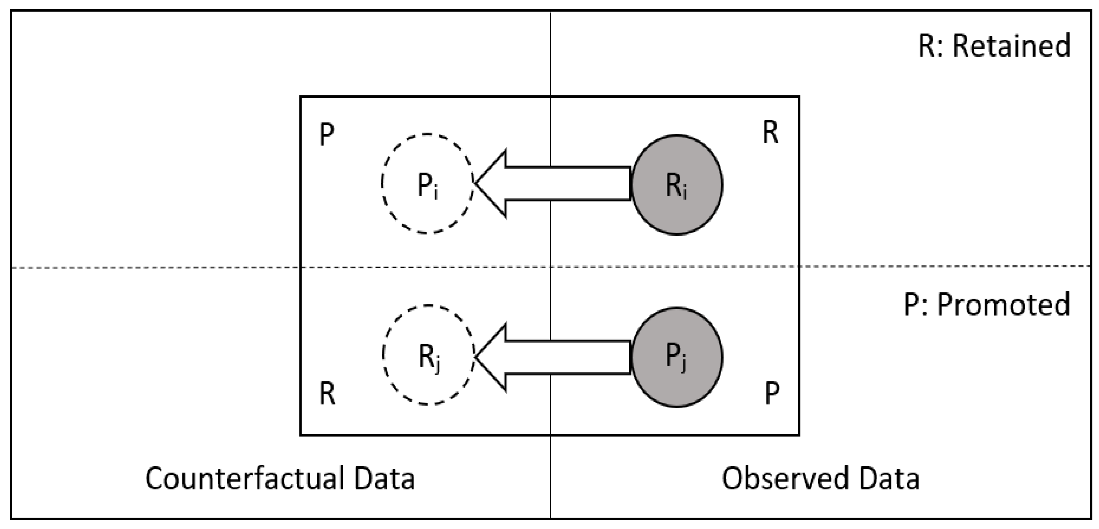
2.1. Research Setting

Throughout this paper, we assume a causal inference has been made based on a regression model and an observational study which has two groups (i.e., the treatment group and the control group). We further assume the inference is made based on a representative sample such that its internal validity is the major concern. In this paper, average treatment effect is estimated by the beta coefficient (we define ${\beta }_W$ as the beta coefficient in order to standardize the discussion, but one can always apply our framework to an ordinary regression coefficient of the treatment indicator with the necessary transformation) of the treatment indicator W, i.e., ${\widehat{\beta }}_W$ in the regression $Y={\beta }_0+{\beta }_{W}W+{\beta }_1{Z}_1+\cdots +{\beta }_p{Z}_p+\epsilon$, where W = 1 for treatment cases, 0 for the control. We assume the above regression model is a classical linear regression model (CLRM), i.e., $\epsilon$ follows normal distribution with the common variance ${\sigma }^2$. The covariates $Z_1,Z_2,\cdots ,Z_p$ included in the regression model are typically needed for the unconfoundedness assumption to be plausible. We note that the estimated propensity scores and/or the propensity score design (propensity score matched pairs or strata) could be controlled in the above regression model as well.

2.2. Definitions

Definition 1. 

The counterfactual data for a subject refers to the imaginary observation which consists of his/her counterfactual outcome (instead of the observed outcome), his/her counterfactual treatment status (i.e., his/her treatment status is different than what he/she actually received) and his/her values for the covariates controlled in the regression model. Thus, there are no variables confounded with treatment assignment when both the counterfactual data and the observed data are included [10].

Example 1. 

In [25], the counterfactual data for John who was retained in the kindergarten would be John’s potential reading score had he been promoted to first grade, and the covariates (e.g., gender, race, socioeconomic status) were identical to those in his observation.

Figure 1 illustrates the conceptualization of the counterfactual data in [25] for the regression estimator. Let $Y_{r,i}^{ob}$ and $Y_{p,j}^{ob}$ be the observed reading scores for the retained students and the promoted students, respectively, and their corresponding counterfactual reading scores are denoted by $Y_{p,i}^{un}$ and $Y_{r,j}^{un}$. $R_i$ denotes the observed data for any student $i$ who was retained in the kindergarten and is written as $\left[Y_{r,i}^{ob},W=1,Z_{1,i},Z_{2,i},\cdots ,Z_{p,i}\right]$, and the corresponding counterfactual data $P_i$ should be $\left[Y_{p,i}^{un},W=0,Z_{1,i},Z_{2,i},\cdots ,Z_{p,i}\right]$. Likewise, $P_j$ denotes the observed data of any student $j$ who was promoted to the first grade and is written as $\left[Y_{p,j}^{ob},W=0,Z_{1,j},Z_{2,j},\cdots ,Z_{p,j}\right]$, and the corresponding counterfactual data $R_j$ is $\left[Y_{r,j}^{un},W=1,Z_{1,j},Z_{2,j},\cdots ,Z_{p,j}\right]$. By definition, the observed sample consists of the observed data $P_j$ and $R_i$, whereas the counterfactual data $P_i$ and $R_j$ are missing from the observed sample. Furthermore, we define ${\overline{Y}}_t^{un}$ and ${\overline{Y}}_c^{un}$ as the means of $Y_{r,j}^{un}$ and $Y_{p,i}^{un}$, respectively, i.e., they denote the mean counterfactual outcomes of the control subjects (the promoted students) and the treated subjects (the retained students). We will show the PIVR is a function of them, conditional on the observed sample.

Definition 2. 

We define the following observed sample statistics required for computing the PIVR: (i) ${\overline{Y}}_t^{ob}$ which denotes the mean observed outcome of the treated subjects (the retained students); (ii) ${\overline{Y}}_c^{ob}$ which denotes the mean observed outcome of the control subjects (the promoted students); (iii) ${\widehat{\sigma }}_t^2$ and ${\widehat{\sigma }}_c^2$ which denote the variances of the observed outcomes of the treated and control subjects, respectively; (iv) $n^{ob}$ which denotes the observed sample size; (v) π which denotes the proportion of the treated subjects in the observed sample; (vi) ${\widehat{R}}^2$ denotes the R-square for the regression model defined in the Section 2.1 based on the observed sample. We also use ${\widehat{\beta }}_W^{ob}$ to denote the estimated beta coefficient of W based on the observed sample.

Definition 3. 

The ideal sample refers to the combination of the observed data and the counterfactual data for all sampled subjects. Based on the definition of the ideal sample, we define ${\overline{Y}}_t^{id}$ and ${\overline{Y}}_c^{id}$ as the mean of all the outcomes under the treatment and the mean of all the outcomes under the control, respectively, should all potential outcomes become available (in our conceptualization). Furthermore, we use ${\widehat{\beta }}_W^{id}$ and $se\left({\widehat{\beta }}_W^{id}\right)$ to denote the estimated beta coefficient of W and its standard error based on the ideal sample. It is noteworthy that the ideal sample is a fixed sample pertains to the same observed subjects, and each subject has both the observed and counterfactual data, i.e., both potential outcomes are thought to be available for every subject in the ideal sample. Therefore, the central task for forming the ideal sample is to conceptualize the counterfactual outcomes, given the observed sample and domain knowledge. When the unconfoundedness assumption fails, the counterfactual data are distinct from the observed data, implying a gap between the observed outcomes and the counterfactual outcomes. Therefore, to evaluate the robustness of a causal inference, one needs to conceptualize all the plausible values of the counterfactual outcomes and how likely the causal inference can still hold conditional on those plausible values. Essentially, our conceptual framework is built on the relationship between the counterfactual outcomes and the null hypothesis significance testing (NHST) result based on the ideal sample, given a conceptual knowledge about the plausible values of the counterfactual outcomes.

3. The Probability of a Robust Inference for Internal Validity in Regression

The PIVR is rooted in the context of null hypothesis significance testing (NHST). To decide whether there is an effect, the null hypothesis $H_0:{\beta }_W=0$ is tested against the alternative hypothesis $H_a:{\beta }_W\ne 0$ (our framework should be easily modified for constants other than 0 or one-sided hypothesis). The PIVR is meaningful only if the null hypothesis has already been rejected based on the observed sample. Since the counterfactual outcomes might be distinct from the observed outcomes, it is natural to wonder whether the null hypothesis would be rejected again based on the ideal sample if the counterfactual outcomes were known, evidencing their inference is robust for internal validity.

Drawing on the above intuition, the probability of a robust inference for internal validity in regression (PIVR) is defined as follows for an observed significant ${\widehat{\beta }}_W^{ob}$, based on the ideal sample:

$$\mathrm{PIVR}=P({\widehat{\beta }}_W^{id} \mathrm{is} \mathrm{significant} | {\widehat{\beta }}_W^{ob} \mathrm{is} \mathrm{significant})$$

(1)

This means that the PIVR evaluates the probability of rejecting the null hypothesis $H_0$ again based on the ideal sample, given the fact that $H_0$ has already been rejected based on the observed sample, if the counterfactual data are included. It is important to note that ${\widehat{\beta }}_W^{id}$ and ${\widehat{\beta }}_W^{ob}$ should have the same sign to ensure the conclusion from rejecting $H_0$ is consistent [20]. For a NHST that is built on either normal or student’s t-distribution, the PIVR has the following relationship with the T-ratio $T=\frac{{\widehat{\beta }}_W^{id}}{se\left({\widehat{\beta }}_W^{id}\right) }$:

If ${\widehat{\beta }}_W^{ob}$ is significantly positive:

$${\mathsf{\Phi }}^{-1}\left(PIVR\right)=T-C$$

(2)

If ${\widehat{\beta }}_W^{ob}$ is significantly negative:

$${\mathsf{\Phi }}^{-1}\left(PIVR\right)=C-T$$

(3)

where C is the critical value and ${\mathsf{\Phi }}^{-1}$ is the inverse of the standard normal CDF. We caution readers that (2) and (3) are approximately true for studies with small sample sizes and C is typically chosen based on the level of significance $\alpha$, i.e., C could be written as $Z_{1-\alpha /2}$ for a significantly positive ${\widehat{\beta }}_W^{ob}$ or $Z_{\alpha /2}$ for a significantly negative ${\widehat{\beta }}_W^{ob}$ [21]. For example, C would be 1.96 if ${\widehat{\beta }}_W^{ob}$ is significantly positive and the level of significance is 0.05. The Equations (2) and (3) above uncover that the PIVR is the statistical power of retesting the null hypothesis $H_0:{\beta }_W=0$ versus the alternative hypothesis $H_a:{\beta }_W={\widehat{\beta }}_W^{id}$ based on the ideal sample, as the statistical power has the exactly same expression (i.e., if one replace the PIVR with the statistical power in the Equations (2) and (3)).

4. The Relationship between the PIVR and the Counterfactual Outcomes

The relationship between the PIVR and the two mean counterfactual outcomes (i.e., ${\overline{Y}}_t^{un}$: the mean counterfactual outcome for the control subjects had they switched to the treatment group and ${\overline{Y}}_c^{un}$: the mean counterfactual outcome for the treated subjects had they switched to the control group) is derived as follows:

Theorem 1. 

The probit link of the PIVR is a function of ${\overline{Y}}_t^{un}$ and ${\overline{Y}}_c^{un}$, conditional on the observed sample statistics ${\widehat{R}}^2,n^{ob},{\overline{Y}}_t^{ob},{\overline{Y}}_c^{ob},$${\widehat{\sigma }}_t^2$, ${\widehat{\sigma }}_c^2,\pi$ as well as the critical value C for rejecting the null hypothesis. Specifically, if ${\widehat{\beta }}_W^{ob}$ is significantly positive, we have:

$${\mathsf{\Phi }}^{-1}\left(PIVR\right)=\frac{\sqrt{2n^{ob}}}{\sqrt{1-R^2}}\frac{{\overline{Y}}_t^{id}-{\overline{Y}}_c^{id}}{\sqrt{2{\widehat{\sigma }}_t^2+2\pi \left(1-\pi \right)\left[\left({\overline{Y}}_t^{un}-{\overline{Y}}_t^{ob}\right){ }^2+\left({\overline{Y}}_c^{un}-{\overline{Y}}_c^{ob}\right){ }^2\right]+2{\widehat{\sigma }}_c^2+{\left({\overline{Y}}_t^{id}-{\overline{Y}}_c^{id}\right)}^2}}-C$$

(4)

If ${\widehat{\beta }}_W^{ob}$ is significantly negative, we have:

$${\mathsf{\Phi }}^{-1}\left(PIVR\right)=C-\frac{\sqrt{2n^{ob}}}{\sqrt{1-R^2}}\frac{{\overline{Y}}_t^{id}-{\overline{Y}}_c^{id}}{\sqrt{2{\widehat{\sigma }}_t^2+2\pi \left(1-\pi \right)\left[\left({\overline{Y}}_t^{un}-{\overline{Y}}_t^{ob}\right){ }^2+\left({\overline{Y}}_c^{un}-{\overline{Y}}_c^{ob}\right){ }^2\right]+2{\widehat{\sigma }}_c^2+{\left({\overline{Y}}_t^{id}-{\overline{Y}}_c^{id}\right)}^2}}$$

(5)

where ${\overline{Y}}_t^{id}$ and ${\overline{Y}}_c^{id}$ are:

$$\begin{gathered} {\overline{Y}}_t^{id}=\left(1-\pi \right){\overline{Y}}_t^{un}+\pi {\overline{Y}}_t^{ob} \\ {\overline{Y}}_c^{id}=\pi {\overline{Y}}_c^{un}+\left(1-\pi \right){\overline{Y}}_c^{ob} \end{gathered}$$

(6)

(Proof in Supplementary Material).

Theorem 1 (i.e., the Equations (4) and (5)) is derived based on the key results offered by (2) and (3), that is, the complex term in (4) (or (5)) is the expression of $T=\frac{{\widehat{\beta }}_W^{id}}{se\left({\widehat{\beta }}_W^{id}\right) }$. As normality is assumed for testing $H_0:{\beta }_W=0$ versus $H_a:{\beta }_W={\widehat{\beta }}_W^{id}$ based on the ideal sample, one can then derive (4) and (5) according to the definition of the PIVR. $R^2$ denotes the R-square for the regression of Y on W and Z in the ideal sample. For convenience, we assume the R-square of the aforementioned regression model based on the ideal sample is the same as its counterpart based on the observed sample, i.e., we assume $R^2={\widehat{R}}^2$ so that we can obtain the exact form of (4) or (5) based on the observed sample. It is clear that the PIVR is conditional on the values of mean counterfactual outcomes ${\overline{Y}}_t^{un}$ and ${\overline{Y}}_c^{un}$ besides the observed sample statistics, so they need to be conceptualized. ${\overline{Y}}_t^{id}$ is weighted average of ${\overline{Y}}_t^{un}$ and ${\overline{Y}}_t^{ob}$, with the weight defined by $\pi$. For the example of the effect of kindergarten retention on reading achievement [25], ${\overline{Y}}_t^{un}$ is the mean reading score for the promoted students had they all been retained instead and ${\overline{Y}}_t^{ob}$ is the observed mean reading score for the retained students, with the weight defined by the proportion of students who were retained in the observed sample. Likewise, ${\overline{Y}}_c^{id}$ is weighted average of the mean reading score for the retained students had they all been promoted instead (${\overline{Y}}_c^{un}$) and the observed mean reading score for the promoted students (${\overline{Y}}_c^{ob}$). Interestingly, Theorem 1 also has a Bayesian interpretation where ${\overline{Y}}_t^{un}$ and ${\overline{Y}}_c^{un}$ characterize the counterfactual data that defines the prior distribution of the causal parameter [19,28,29].

Theorem 1 entails the use of critical value C as the decision threshold for rejecting the null hypothesis $H_0:{\beta }_W=0$, which is mostly appropriate for NHST. However, we note that the decision threshold for rejecting the null hypothesis $H_0$ could also be a fixed value that is pragmatically set based on transaction cost and/or policy implications [20]. For example, it might be sensible to use a fixed effect size (like 1) as the decision threshold for [25], i.e., the null hypothesis $H_0$ would not be rejected unless the effect size exceeds 1, considering the substantial cost of implementing or revoking the policy of kindergarten retention [30]. Under such circumstances, the relationship between the PIVR and the mean counterfactual outcomes would change so that it depends on the actual decision threshold rather than the critical value C.

The aforementioned relationships between the PIVR and the mean counterfactual outcomes allow for one to compute the PIVR based on specific values of ${\overline{Y}}_t^{un}$ and ${\overline{Y}}_c^{un}$. In the example of [25], if one believes the mean reading score of the promoted students had they been retained instead (i.e.,${\overline{Y}}_t^{un}$) was equal to the mean of their observed reading score (45.78) and that the mean reading score of the retained students had they been promoted instead (i.e., ${\overline{Y}}_c^{un}$) was equal to the grand mean (45.2), ${\widehat{\beta }}_W^{id}$ would follow normal distribution with mean as −0.022 and standard deviation as 0.006. As a result, the PIVR which is $P({\widehat{\beta }}_W^{id}<-1.96\times .006)$ would then be 0.92. Furthermore, inferences about the PIVR are possible based on joint distributions of ${\overline{Y}}_t^{un}$ and ${\overline{Y}}_c^{un}$. For example, assuming ${\overline{Y}}_t^{un}$ follows the uniform distribution in [45, 45.78] and ${\overline{Y}}_c^{un}$ follows the uniform distribution in [36.77, 45.78], the expected value of the PIVR would be 0.86 and its 95% confidence interval would be [0.14, 1.00] across all possible distributions of ${\widehat{\beta }}_W^{id}$ defined by ${\overline{Y}}_t^{un}$ and ${\overline{Y}}_c^{un}$. We will detail such analysis in the next section.

5. Example: The Effect of Kindergarten Retention on Reading Achievement

5.1. Overview

Kindergarten retention is estimated to affect 7 percent to 15 percent of the student population in the U.S. and cost USD 20 billion dollars annually [30,31]. It also imposes physical and psychological costs on retained students, and thus has been a controversial issue for many years. To examine the effectiveness of kindergarten retention, [25] conducted propensity score analysis using nationally representative data from the Early Childhood Longitudinal Study (ECLS) and a rich set of covariates such as student background information, psychological/motivational measures, as well as pretests. Based on a multilevel model which controlled for both the logit of propensity scores as well as the propensity score strata, they estimated the effect of kindergarten retention on students’ reading achievement as −9.01 with standard error of 0.68, which amounted to an effect size of 0.67. Ultimately, Hong and Raudenbush concluded that retention reduces achievement: “children who were retained would have learned more had they been promoted (page 200)”.

However, the internal validity of [25] is open to debate since it relied on the unconfoundedness assumption, which required all potential confounding variables to be controlled by their propensity score model. Nonetheless, [20] has argued that some potential confounders, such as key measures of cognitive ability and emotional disposition, might still be missing in their propensity score model and thus may have potentially biased the estimates. If an omitted confounder were negatively correlated with kindergarten retention and positively correlated with reading achievement, the estimate of kindergarten retention could be downwardly biased, and thus their inference would be invalidated if such omitted confounder was taken into account.

To address the above concern such that researchers and policymakers may evaluate the robustness of an inference with questionable internal validity, we develop an analytical procedure based on the relationship between the PIVR and the mean counterfactual outcomes in Theorem 1. Specifically, this analytical procedure has six steps: (i) obtain the required sample statistics, (ii) choose critical value C (here we assume one use a statistical threshold, but a decision threshold could be a non-statistical one), (iii) obtain the relationship between the PIVR and the mean counterfactual outcomes, (iv) specify a joint distribution about the mean counterfactual outcomes, (v) calculate the expected value and confidence interval for the PIVR, and (vi) evaluate the robustness based on the expected value of the PIVR.

5.2. Quantifying the Robustness of the Inference of Hong and Raudenbush (2005) [25]

(i)

Obtain the required sample statistics: The required observed sample statistics ${\widehat{R}}^2,n^{ob},{\overline{Y}}_t^{ob},{\overline{Y}}_c^{ob},$ ${\widehat{\sigma }}_t^2$, ${\widehat{\sigma }}_c^2,\pi$ are obtained as follows: ${\widehat{R}}^2=0.36,n^{ob}=7639,{\overline{Y}}_t^{ob}=36.77, {\overline{Y}}_c^{ob}=45.78,{\widehat{\sigma }}_t^2=143.26,{\widehat{\sigma }}_c^2=138.83,\pi =0.0617$ [20].

(ii)

Choose critical value C: Given that [25] reported that kindergarten retention had a significant negative effect on reading achievement, we decided to choose C as −1.96 which means the level of significance is 0.05 for rejecting the null hypothesis $H_0:{\beta }_W=0$.

(iii)

Obtain the relationship between the PIVR and the mean counterfactual outcomes: Plugging the observed sample statistics and the critical value above into (5), the PIVR is the probit function of the mean counterfactual reading score for the retained students had they been promoted instead (i.e., ${\overline{Y}}_c^{un}$) and the mean counterfactual reading score for the promoted students had they been retained instead (i.e.,${\overline{Y}}_t^{un}$) as follows:

$${\mathsf{\Phi }}^{-1}\left(PIVR\right)=-1.96-\frac{109.25\times \left(0.9383{\overline{Y}}_t^{un}-0.0617{\overline{Y}}_c^{un}-40.69\right)}{\sqrt{564.18+0.116\times \left[\left({\overline{Y}}_t^{un}-36.77\right){ }^2+\left({\overline{Y}}_c^{un}-45.78\right){ }^2\right]+{\left(0.9383{\overline{Y}}_t^{un}-0.0617{\overline{Y}}_c^{un}-40.69\right)}^2}}$$

(7)

(iv)

Specify a joint distribution about the mean counterfactual outcomes: This step requires one to form a joint distribution about the two mean counterfactual outcomes. In general, the distributional belief about the mean counterfactual outcomes should be based on counterfactual thought experiments with explicit justifications. It is recommended that one choose the ranges of the mean counterfactual outcomes based on domain knowledge and literature, and that those ranges should only include the unfavorable scenarios, i.e., the values of mean counterfactual outcomes that would make the observed results less significant. As a rule of thumb, one can then form uniform distributions based on the ranges of the mean counterfactual outcomes.

In this example, the counterfactual thought experiments are carried out by conceptualizing the questions “what would the mean reading score of the promoted students be had they been retained instead (i.e.,${\overline{Y}}_t^{un}$)” and “what would the mean reading score of the retained students be had they been promoted instead (i.e., ${\overline{Y}}_c^{un}$)”. Those questions can be answered by reflecting on the counterfactual outcomes based on belief about the average retention (treatment) effects for the retained students and for the promoted students, identified by ${\overline{Y}}_t^{ob}-{\overline{Y}}_c^{un}$ and ${\overline{Y}}_t^{un}-{\overline{Y}}_c^{ob}$, respectively. For illustration, we compare two different joint distributions about ${\overline{Y}}_t^{un}$ and ${\overline{Y}}_c^{un}$.

The first joint distribution: Given the estimated average retention effect for the retained students was significantly negative (36.77 − 45.78 = −9.01), it is reasonable to think kindergarten retention also had a negative impact on reading achievement for the promoted students, which is also supported by the literature [32,33,34]. In addition, we believed that the original estimate of average retention effect for the retained students, which was −9, was overestimated such that the inference of [25] could be invalidated. This means ${\overline{Y}}_c^{un}$ should be no smaller than ${\overline{Y}}_t^{ob}$ (which was 36.77) and no larger than ${\overline{Y}}_c^{ob}$ (which was 45.78). Furthermore, we only focused on small average retention effects for the promoted students, i.e., ${\overline{Y}}_t^{un}$ was slightly smaller than ${\overline{Y}}_c^{ob}$ which was 45.78, as larger effects for the promoted students would increase the effect size and make the discussion about the PIVR less practical. As a result, we assumed ${\overline{Y}}_t^{un}$ followed the uniform distribution in [45, 45.78] and ${\overline{Y}}_c^{un}$ followed the uniform distribution in [36.77, 45.78]. This indicates that ${\widehat{\beta }}_W^{id}$ follows a normal distribution whose mean is in the range [−0.054, 0] and standard deviation is 0.0065.

The second joint distribution: The purpose of having a second joint distribution of ${\overline{Y}}_t^{un}$ and ${\overline{Y}}_c^{un}$ is to illustrate the impact of tighter bounds of ${\overline{Y}}_t^{un}$ and ${\overline{Y}}_c^{un}$ on inferences about the PIVR [35,36]. For this purpose, we assumed ${\overline{Y}}_t^{un}$ followed the uniform distribution in [45, 45.5] and ${\overline{Y}}_c^{un}$ followed the uniform distribution in [36.77, 45.2], which means the ranges of ${\overline{Y}}_t^{un}$ and ${\overline{Y}}_c^{un}$ were slightly narrowed in the second joint distribution, comparing to the first joint distribution. This indicates ${\widehat{\beta }}_W^{id}$ follows a normal distribution whose mean is in the range [−0.052, −0.011] and standard deviation is 0.0065.

(v)

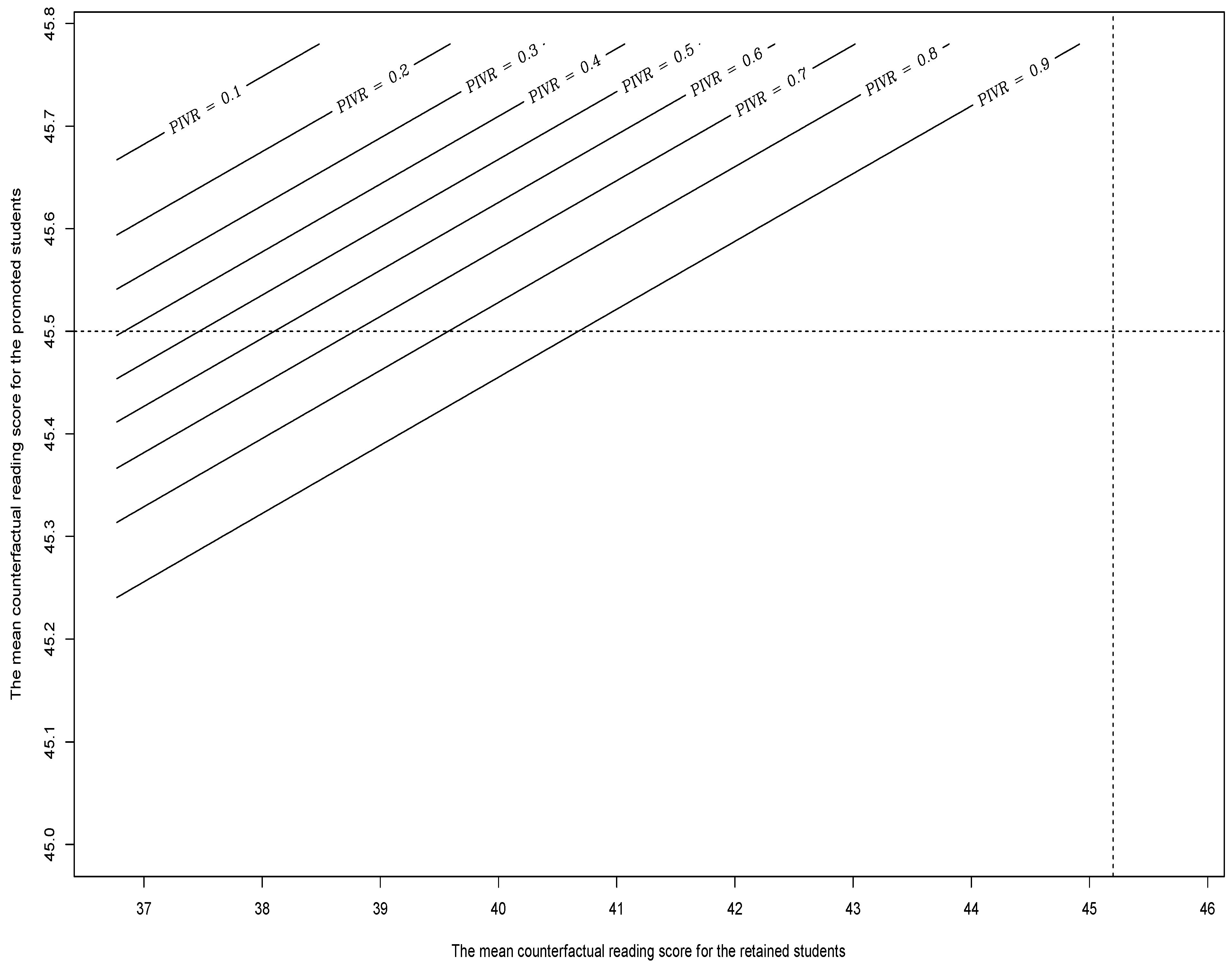
Calculate the expected value and confidence interval for the PIVR: Figure 2 illustrates the levels of the PIVR for [25] based on the first joint distribution of ${\overline{Y}}_t^{un}$ and ${\overline{Y}}_c^{un}$. The distribution of the PIVR is approximated by the following process: 1—repeatedly draw random values from the first joint distribution; 2—obtain the corresponding normal distribution for ${\widehat{\beta }}_W^{id}$ (specifically, the mean of such normal distribution); 3—compute the PIVR which is $P({\widehat{\beta }}_W^{id}<-1.96\times 0.0065)$ based on the normal distribution obtained in the second step. We can then derive the expected value of the PIVR as 0.86 and its 95% confidence interval as [0.14, 1.00], for the first joint distribution. This means the chance that the inference of [25] is robust for internal validity is expected to be 86% based on the first joint distribution. For the second joint distribution of ${\overline{Y}}_t^{un}$ and ${\overline{Y}}_c^{un}$, we derive the expected value of the PIVR as 0.96 and its 95% confidence interval as [0.66, 1.00] by a similar fashion. This suggests the chance that Hong and Raudenbush’s inference is robust for internal validity is expected to be 96% based on the second joint distribution, and we have higher confidence about the robustness of Hong and Raudenbush’s inference compared to the results obtained based on the first joint distribution.

(vi)

Evaluate the robustness based on the expected value of the PIVR: Given the PIVR can be interpreted as the statistical power of retesting the null hypothesis $H_0:{\beta }_W=0$ based on the ideal sample, we use PIVR = 0.8 as the threshold which is often used for strong statistical power [37,38]. Consequently, we conclude that the inference of [25] is expected to be robust given the first joint distribution of ${\overline{Y}}_t^{un}$ and ${\overline{Y}}_c^{un}$, as the expected value 0.86 exceeds the threshold 0.8. We conclude again that the inference of [25] is expected to be robust given the second joint distribution of ${\overline{Y}}_t^{un}$ and ${\overline{Y}}_c^{un}$, as the expected value 0.96 exceeds the threshold 0.8. We caution readers that the above conclusions might not hold if a different joint distribution ${\overline{Y}}_t^{un}$ and ${\overline{Y}}_c^{un}$ and/or a different threshold for strong statistical power is chosen for PIVR analysis.

The above PIVR calculations (i.e., the step 4 and 5) can be conceptualized as the process of retesting the null hypothesis $H_0:{\beta }_W=0$ versus the alternative hypothesis $H_a:{\beta }_W={\widehat{\beta }}_W^{id}$ iteratively based on different values of ${\overline{Y}}_t^{un}$ and ${\overline{Y}}_c^{un}$ drawn from their joint distribution. Based on Theorem 1, one can easily calculate the PIVR which can be interpreted as the statistical power of the above hypothesis (re)testing, conditional on values of ${\overline{Y}}_t^{un}$ and ${\overline{Y}}_c^{un}$. We illustrate the interpretation of the PIVR as the statistical power by assuming ${\overline{Y}}_c^{un}=45.2$ which is the grand mean of the test scores in [25] in the Supplementary Material Figure S1. As ${\overline{Y}}_t^{un}$ decreases, the PIVR increases as the effect size grows. Based on a joint distribution of ${\overline{Y}}_t^{un}$ and ${\overline{Y}}_c^{un}$, which effectively conveys one’s belief about the unconfoundedness assumption, PIVR analysis can be thought of as power analysis for the NHST $H_0:{\beta }_W=0$ versus $H_a:{\beta }_W={\widehat{\beta }}_W^{id}$ conditional on one’s belief (in the form of a joint distribution of ${\overline{Y}}_t^{un}$ and ${\overline{Y}}_c^{un}$). An inference that is robust for internal validity should, on average, have a strong statistical power based on a joint distribution of ${\overline{Y}}_t^{un}$ and ${\overline{Y}}_c^{un}$.

6. Discussion

Focusing on the beta coefficient of treatment indicator, we began by defining the counterfactual data, and the ideal sample consisted of the counterfactual data and the observed data. The assessment of internal validity should be based on the ideal sample, and for null hypothesis significance testing (NHST) this means one should test the null hypothesis (versus the alternative hypothesis) based on the ideal sample and check if the result is consistent with the testing result based on the observed sample. The probability of a robust inference for internal validity in regression, i.e., the PIVR, is thus defined as the probability of rejecting the null hypothesis $H_0:{\beta }_W=0$ again based on the ideal sample, given that it has been rejected based on the observed sample. Internal validity is evaluated by estimating the mean and 95% confidence interval of the PIVR based on a joint distribution of the mean counterfactual outcomes.

It is worth clarifying that the ideal sample is formed by adding counterfactual outcomes to the observed sample/data, and therefore the ideal sample essentially addresses missing data issue (i.e., the counterfactuals are missing) rather than sampling issue (i.e., the observed sample of individuals or subjects remain fixed for the ideal sample). The ideal sample is typically meaningful, after one obtains a significant result based on the observed sample and starts to question the internal validity of the result. The robustness/internal validity of the result would then have to be evaluated based on plausible values of the counterfactual outcomes, which in our approach need to be conceptualized by a thought experiment with explicit justifications. By this logic, our robustness indices, the PIVR, inform the probability of rejecting the null hypothesis again based on the ideal sample (as the same null hypothesis has already been rejected based on the observed sample). It should be clear that the sole driver of the PIVR is the mean counterfactual outcomes from the Theorem 1, as the ideal sample consists of the observed sample which is always fixed and the missing counterfactual outcomes which should be varying within certain limits.

There are similar approaches designed for internal validity assessment in different disciplines. For statisticians, sensitivity analysis has been considered as an essential part in causal inference [7,8,17,39,40,41]. In sensitivity analysis, one would evaluate the impact of a missing confounder on regression estimates and nonparametric tests by conceptually connecting the assumption of unconfoundedness to the plausibility of random assignment in matched pairs. Other notable work in sensitivity analysis has slightly different perspectives but all starts with the potential failure of the unconfoundedness assumption [42,43,44,45,46,47]. In particular, Bayesian sensitivity analysis [48,49,50,51] utilizes a Bayesian framework where the models for the outcome and the unmeasured confounder are parameterized so as to identify the key confounding parameters. Bayesian sensitivity analyses typically involves a data augmentation step that allows for one to repeatedly impute missing values for the unobserved confounder and a prior specification step that brings more flexibility; thus, unobserved confounders can be taken into account given a joint posterior distribution of the confounding and treatment effect parameters. Robustness indices of causal inferences have been applied to educational research [19,21,52]. Those indices quantify the strength of internal validity in terms of the impact of an unmeasured confounding variable, or the proportion of observed cases can be replaced by null cases that an inference can withstand. Bounds of treatment effect are found more often in the field of economy [36,37,53,54]. They can be obtained by imposing further (detailed) assumptions on the counterfactuals and can be tightened by making the assumption(s) more informative. Notably, Manski’s bounds of treatment effect are nonparametric and built on situations where the unconfoundedness assumption does not hold. Manski’s bounds also inform the worth of a causal inference through exploring loss-based alternatives rooted in the context of program evaluation. In the field of psychology, probabilities of reproducibility become increasingly popular as they are designed to protect readers from misguidance and misinterpretation of p-values [55,56,57,58,59]. The probabilities of reproducibility are driven by the reproducibility of a scholarly finding rather than its statistical significance, thus becoming tools for tackling the reproducibility crisis [60,61].

Different from the aforementioned similar approaches, our approach is built on thought experiments and domain knowledge/beliefs about the counterfactual outcomes rather than additional models/assumptions about the treatment assignment (such as propensity scores). The purpose of having thought experiments/beliefs about the counterfactual outcomes (instead of models/assumptions) is that one often can infer what would happen in a counterfactual scenario based on domain knowledge, which arguably should be the core of causal inference. The PIVR typically requires much fewer modeling/parametric assumptions about the outcome and treatment assignment compared to sensitivity analysis or Bayesian sensitivity analysis. Compared to robustness indices and Manski’s bounds, the PIVR asks for a thought experiment about all plausible counterfactual outcomes based on explicit justifications, and therefore it is more comprehensive and concrete. Another difference is that the PIVR is a probabilistic index while the robustness indices and Manski’s bounds are not (the robustness indices are thresholds and the Manski’s bounds are bounding the treatment effects). The PIVR is actually the probability of replicating a significant result in an observational study for the ideal sample, and it is similar to $p_{rep}$ [57,62], which is the probability of obtaining an effect with the same sign as the observed one. Different from $p_{rep}$ and other probabilities of reproducibility, the PIVR takes counterfactual outcomes into consideration and therefore it is not a function of p-value. Therefore, it does not inherit any of the limitations associated with p-value as most proposed probabilities of reproducibility do [63].

The scholarly significance of this study manifests in three aspects: First, it prompts researchers to conceptualize the counterfactual outcomes and form distributional beliefs about them. This will foster critical thinking as well as scientific discourse about internal validity since people can use the PIVR to understand under what circumstances and to what degree internal validity will be robust using regression. Thought experiments can be carried out in contexts that are similar or different from the study of interest to facilitate the conceptualization of the counterfactual outcomes. For our example, one can imagine a direct comparison between two cohorts of students from the same school district, i.e., a comparison between one cohort from a school with retention policy and another cohort from a school without such policy in the same district. One can also alter the criteria of retention/promotion and attempt to infer the potential outcomes under those scenarios. Lastly, one can even imagine the retention/promotion policy to be enforced in a secondary school/university and conceptualize its impact. Second, the PIVR can be interpreted as the statistical power of retesting the null hypothesis $H_0:{\beta }_W=0$ versus the alternative hypothesis $H_a:{\beta }_W={\widehat{\beta }}_W^{id}$ based on the ideal sample. Therefore, it offers an intuitive interpretation of the robustness of an inference based on NHST. We caution readers that the PIVR does not inform true effect or model validity for a particular study, rather it is used to indicate when and to what degree a significant hypothesis testing result can still hold based on one’s belief about the counterfactuals. Third, the PIVR is pragmatic as it quantifies the impact of the counterfactual outcomes (and thus internal validity) on decision-making, given a distributional belief and a decision threshold chosen by researcher(s).

There are notable limitations associated with our approach: First, our approach requires a distributional belief about the mean counterfactual outcomes, which could be challenging to obtain and even unfeasible in some cases. As we have pointed out, such distributional belief should be derived based on domain knowledge/literature and only cover the unfavorable scenarios where the significance of the observed results would be compromised. On the other hand, an unjustified, non-specific, subjective belief may put the causal discourse at risk and render the robustness analysis meaningless. Second, our approach was developed mainly for CLRM and therefore may not be appropriate for studies with discrete outcomes and nonlinear models. Third, our approach is arguably an abstract approach as it is directly built on counterfactual thought experiments (and the conceptualized plausible values for mean counterfactual outcomes), and we did not make further inquiries as to why the counterfactual outcomes change, which may be due to an omitted confounder, the violation of stable unit treatment value assumption (SUTVA), or measurement error. Remarkably, SUTVA is a major challenge for making causal inference in educational research, as students frequently interact with each other [9]. For our example, this means the academic progress of a student might be related to his/her reaction to retention/promotion as well as other students’ reactions. Therefore, the PIVR is inadequate for evaluating a specific causal mechanism or data-generating process (DGP), such as the existence of an interaction between the treatment and a missing confounder, and it is only appropriate for evaluating the robustness of a conclusion drawn from NHST. In light of the above concerns, a power of test may be needed to study the performance of the PIVR as well as specific statistical approach that was engaged in causal inference [64].

References

1. Gelman, A.; Hill, J. Data Analysis Using Regression and Multilevel/Hierarchical Models; Cambridge University Press: New York, NY, USA, 2006. [Google Scholar]
2. Imbens, G.W.; Rubin, D.B. Causal Inference for Statistics, Social, and Biomedical Sciences: An Introduction; Cambridge University Press: New York, NY, USA, 2015. [Google Scholar] [CrossRef]
3. Morgan, S.L.; Winship, C. Counterfactuals and Causal Inference; Cambridge University Press: New York, NY, USA, 2015. [Google Scholar]
4. Murnane, R.J.; Willett, J.B. Methods Matter: Improving Causal Inference in Educational and Social Science Research; Oxford University Press: New York, NY, USA, 2011. [Google Scholar]
5. Shadish, W.R.; Cook, T.D.; Campbell, D.T. Experimental and Quasi-Experimental Designs for Generalized Causal Inference; Houghton Mifflin: New York, NY, USA, 2002. [Google Scholar]
6. Imai, K.; King, G.; Stuart, E.A. Misunderstandings between experimentalists and observationalists about causal inference. J. R. Stat. Soc. Ser. A Stat. Soc. 2008, 171, 481–502. [Google Scholar] [CrossRef]
7. Rosenbaum, P.R. Observational Studies; Springer: New York, NY, USA, 2002. [Google Scholar]
8. Rosenbaum, P.R.; Rubin, D.B. Assessing sensitivity to an unobserved binary covariate in an observational study with binary outcome. J. R. Stat. Soc. Ser. B Methodol. 1983, 45, 212–218. [Google Scholar] [CrossRef]
9. Rubin, D.B. Neyman (1923) and causal inference in experiments and observational studies. Stat. Sci. 1990, 5, 472–480. [Google Scholar] [CrossRef]
10. Holland, P.W. Statistics and causal inference. J. Am. Stat. Assoc. 1986, 81, 945–960. [Google Scholar] [CrossRef]
11. Rubin, D.B. For objective causal inference, design trumps analysis. Ann. Appl. Stat. 2008, 2, 808–840. [Google Scholar] [CrossRef]
12. Rubin, D.B. The design versus the analysis of observational studies for causal effects: Parallels with the design of randomized trials. Stat. Med. 2007, 26, 20–36. [Google Scholar] [CrossRef] [PubMed]
13. Schafer, J.L.; Kang, J. Average causal effects from nonrandomized studies: A practical guide and simulated example. Psychol. Methods 2008, 13, 279. [Google Scholar] [CrossRef]
14. Imbens, G.W. Nonparametric estimation of average treatment effects under exogeneity: A review. Rev. Econ. Stat. 2004, 86, 4–29. [Google Scholar] [CrossRef]
15. Rosenbaum, P.R.; Rubin, D.B. The central role of the propensity score in observational studies for causal effects. Biometrika 1983, 70, 41–55. [Google Scholar] [CrossRef]
16. Heckman, J.J. The scientific model of causality. Sociol. Methodol. 2005, 35, 1–97. [Google Scholar] [CrossRef]
17. Rosenbaum, P.R. Sensitivity analysis for certain permutation inferences in matched observational studies. Biometrika 1987, 74, 13–26. [Google Scholar] [CrossRef]
18. Frank, K.A. Impact of a confounding variable on a regression coefficient. Sociol. Methods Res. 2000, 29, 147–194. [Google Scholar] [CrossRef]
19. Frank, K.; Min, K.S. Indices of Robustness for Sample Representation. Sociol. Methodol. 2007, 37, 349–392. [Google Scholar] [CrossRef]
20. Frank, K.A.; Maroulis, S.J.; Duong, M.Q.; Kelcey, B.M. What would it take to change an inference? Using Rubin’s causal model to interpret the robustness of causal inferences. Educ. Eval. Policy Anal. 2013, 35, 437–460. [Google Scholar] [CrossRef]
21. Li, T.; Frank, K.A. The probability of a robust inference for internal validity. Sociol. Methods Res. 2022, 51, 1947–1968. [Google Scholar] [CrossRef]
22. Rubin, D.B. Teaching statistical inference for causal effects in experiments and observational studies. J. Educ. Behav. Stat. 2004, 29, 343–367. [Google Scholar] [CrossRef]
23. Rubin, D.B. Causal inference using potential outcomes: Design, modeling, decisions. J. Am. Stat. Assoc. 2005, 100, 322–331. [Google Scholar] [CrossRef]
24. Sobel, M.E. An introduction to causal inference. Sociol. Methods Res. 1996, 24, 353–379. [Google Scholar] [CrossRef]
25. Hong, G.; Raudenbush, S.W. Effects of kindergarten retention policy on children’s cognitive growth in reading and mathematics. Educ. Eval. Policy Anal. 2005, 27, 205–224. [Google Scholar] [CrossRef]
26. Allen, C.S.; Chen, Q.; Willson, V.L.; Hughes, J.N. Quality of research design moderates effects of grade retention on achievement: A meta-analytic, multilevel analysis. Educ. Eval. Policy Anal. 2009, 31, 480–499. [Google Scholar] [CrossRef]
27. Hong, G. Marginal mean weighting through stratification: Adjustment for selection bias in multilevel data. J. Educ. Behav. Stat. 2010, 35, 499–531. [Google Scholar] [CrossRef]
28. Hoff, P.D. A First Course in BAYESIAN Statistical Methods; Springer Science & Business Media: New York, NY, USA, 2009. [Google Scholar]
29. Li, T. The Bayesian Paradigm of Robustness Indices of Causal Inferences. Doctoral Dissertation, Michigan State University, East Lansing, MI, USA, 2018. Unpublished. [Google Scholar]
30. Alexander, K.L.; Entwisle, D.L.; Dauber, S.L. On the Success of Failure: A Reassessment of the Effects of Retention in the Primary School Grades; Cambridge University Press: New York, NY, USA, 2003. [Google Scholar]
31. Tingle, L.R.; Schoeneberger, J.; Algozzine, B. Does grade retention make a difference? Clear. House A J. Educ. Strateg. Issues Ideas 2012, 85, 179–185. [Google Scholar] [CrossRef]
32. Burkam, D.T.; LoGerfo, L.; Ready, D.; Lee, V.E. The differential effects of repeating kindergarten. J. Educ. Stud. Placed Risk 2007, 12, 103–136. [Google Scholar] [CrossRef]
33. Jimerson, S. Meta-analysis of grade retention research: Implications for practice in the 21st century. Sch. Psychol. Rev. 2001, 30, 420–437. [Google Scholar] [CrossRef]
34. Lorence, J.; Dworkin, G.; Toenjes, L.; Hill, A. Grade retention and social promotion in Texas 1994–1999: Academic achievement among elementary school students. In Brookings Papers on Education Policy; Ravitch, D., Ed.; Brookings Institution Press: Washington, DC, USA, 2002; pp. 13–67. [Google Scholar]
35. Manski, C.F. Nonparametric bounds on treatment effects. Am. Econ. Rev. 1990, 80, 319. [Google Scholar]
36. Manski, C.F. Identification Problems in the Social Sciences; Harvard University Press: Cambridge, MA, USA, 1995. [Google Scholar]
37. Cohen, J. Statistical Power Analysis for the Behavioral Sciences; Lawrence Earlbaum Associates: Hillsdale, NJ, USA, 1988. [Google Scholar]
38. Cohen, J. A power primer. Psychol. Bull. 1992, 112, 155. [Google Scholar] [CrossRef] [PubMed]
39. Rosenbaum, P.R. Dropping out of high school in the United States: An observational study. J. Educ. Stat. 1986, 11, 207–224. [Google Scholar] [CrossRef]
40. Rosenbaum, P.R. Sensitivity analysis for matched case-control studies. Biometrics 1991, 47, 87–100. [Google Scholar] [CrossRef]
41. Rosenbaum, P.R. Design of Observational Studies; Springer: New York, NY, USA, 2010. [Google Scholar]
42. Copas, J.B.; Li, H.G. Inference for non-random samples. J. R. Stat. Soc. Series B Stat. Methodol. 1997, 59, 55–95. [Google Scholar] [CrossRef]
43. Hosman, C.A.; Hansen, B.B.; Holland, P.W. The sensitivity of linear regression coefficients’ confidence limits to the omission of a confounder. Ann. Appl. Stat. 2010, 4, 849–870. [Google Scholar] [CrossRef]
44. Lin, D.Y.; Psaty, B.M.; Kronmal, R.A. Assessing the sensitivity of regression results to unmeasured confounders in observational studies. Biometrics 1998, 54, 948–963. [Google Scholar] [CrossRef] [PubMed]
45. Masten, M.A.; Poirier, A. Identification of treatment effects under conditional partial independence. Econometrica 2018, 86, 317–351. [Google Scholar] [CrossRef]
46. Robins, J.M.; Rotnitzky, A.; Scharfstein, D.O. Sensitivity analysis for selection bias and unmeasured confounding in missing data and causal inference models. In Statistical Models in Epidemiology, the Environment, and Clinical Trials; Springer: New York, NY, USA, 2000; pp. 1–94. [Google Scholar]
47. VanderWeele, T.J. Sensitivity analysis: Distributional assumptions and confounding assumptions. Biometrics 2008, 64, 645–649. [Google Scholar] [CrossRef] [PubMed]
48. Contreras-Reyes, J.E.; Quintero, F.O.L.; Wiff, R. Bayesian modeling of individual growth variability using back-calculation: Application to pink cusk-eel (Genypterus blacodes) off Chile. Ecol. Model. 2018, 385, 145–153. [Google Scholar] [CrossRef]
49. McCandless, L.C.; Gustafson, P.; Levy, A. Bayesian sensitivity analysis for unmeasured confounding in observational studies. Stat. Med. 2007, 26, 2331–2347. [Google Scholar] [CrossRef]
50. McCandless, L.C.; Gustafson, P.; Levy, A.R.; Richardson, S. Hierarchical priors for bias parameters in Bayesian sensitivity analysis for unmeasured confounding. Stat. Med. 2012, 31, 383–396. [Google Scholar] [CrossRef] [PubMed]
51. McCandless, L.C.; Gustafson, P. A comparison of Bayesian and Monte Carlo sensitivity analysis for unmeasured confounding. Stat. Med. 2017, 36, 2887–2901. [Google Scholar] [CrossRef]
52. Busenbark, J.R.; Yoon, H.; Gamache, D.L.; Withers, M.C. Omitted variable bias: Examining management research with the impact threshold of a confounding variable (ITCV). J. Manag. 2022, 48, 17–48. [Google Scholar] [CrossRef]
53. Altonji, J.G.; Elder, T.E.; Taber, C.R. An evaluation of instrumental variable strategies for estimating the effects of catholic schooling. J. Hum. Resour. 2005, 40, 791–821. [Google Scholar] [CrossRef]
54. Manski, C.F.; Nagin, D.S. Bounding disagreements about treatment effects: A case study of sentencing and recidivism. Sociol. Methodol. 1998, 28, 99–137. [Google Scholar] [CrossRef]
55. Boos, D.D.; Stefanski, L.A. P-value precision and reproducibility. Am. Stat. 2011, 65, 213–221. [Google Scholar] [CrossRef] [PubMed]
56. Greenwald, A.; Gonzalez, R.; Harris, R.J.; Guthrie, D. Effect sizes and p values: What should be reported and what should be replicated? Psychophysiology 1996, 33, 175–183. [Google Scholar] [CrossRef] [PubMed]
57. Killeen, P.R. An alternative to null-hypothesis significance tests. Psychol. Sci. 2005, 16, 345–353. [Google Scholar] [CrossRef] [PubMed]
58. Posavac, E.J. Using p values to estimate the probability of a statistically significant replication. Underst. Stat. Stat. Issues Psychol. Educ. Soc. Sci. 2002, 1, 101–112. [Google Scholar] [CrossRef]
59. Shao, J.; Chow, S.C. Reproducibility probability in clinical trials. Stat. Med. 2002, 21, 1727–1742. [Google Scholar] [CrossRef] [PubMed]
60. Camerer, C.F.; Dreber, A.; Forsell, E.; Ho, T.-H.; Huber, J.; Johannesson, M.; Kirchler, M.; Almenberg, J.; Altmejd, A.; Chan, T.; et al. Evaluating replicability of laboratory experiments in economics. Science 2016, 351, 1433–1436. [Google Scholar] [CrossRef] [PubMed]
61. Open Science Collaboration. Estimating the reproducibility of psychological science. Science 2015, 349, aac4716. [Google Scholar] [CrossRef]
62. Iverson, G.J.; Wagenmakers, E.J.; Lee, M.D. A model-averaging approach to replication: The case of prep. Psychol. Methods 2010, 15, 172. [Google Scholar] [CrossRef]
63. Doros, G.; Geier, A.B. Probability of replication revisited: Comment on “An alternative to null-hypothesis significance tests”. Psychol. Sci. 2005, 16, 1005–1006. [Google Scholar] [CrossRef]
64. Li, T.; Lawson, J. A generalized bootstrap procedure of the standard error and confidence interval estimation for inverse probability of treatment weighting. Multivar. Behav. Res. 2023, 2023, 2254541. [Google Scholar] [CrossRef]
Figure 1. Observed and counterfactual data for kindergarten retention for the regression estimator.
Mathematics 12 00388 g001
Figure 2. The contour plot of the PIVR based on the first joint distribution of Y ¯ t u n and Y ¯ c u n   with the x axis representing Y ¯ c u n and the y axis representing Y ¯ t u n   . The first joint distribution is defined based on the belief that the average retention effect for the promoted students should not be positive and the average retention effect for the retained students was overestimated, which means both Y ¯ t u n   and Y ¯ c u n are smaller than 45.78. The vertical and horizontal dashed lines correspond to the upper bounds of Y ¯ t u n   and Y ¯ c u n for the second joint distribution, which are 45.2 and 45.5, respectively. Therefore, the lower-left area (segmented by the dashed lines) represents the second joint distribution of Y ¯ t u n   and Y ¯ c u n .
Mathematics 12 00388 g002
Disclaimer/Publisher’s Note: The statements, opinions and data contained in all publications are solely those of the individual author(s) and contributor(s) and not of MDPI and/or the editor(s). MDPI and/or the editor(s) disclaim responsibility for any injury to people or property resulting from any ideas, methods, instructions or products referred to in the content.