Clade Size Statistics Under Ford’s α-Model

Abstract

Given a labeled tree topology t of n taxa, consider a population P of k leaves chosen among those of t. The clade of P is the minimal subtree $\widehat{P}$ of t containing P, and its size $|\widehat{P}|$ is provided by the number of leaves in the clade. We study distributive properties of the clade size variable $|\widehat{P}|$ considered over labeled topologies of size n generated at random in the framework of Ford’s $\alpha$-model. Under this model, starting from the one-taxon labeled topology, a random labeled topology is produced iteratively by a sequence of $\alpha$-insertions, each of which adds a pendant edge to either a pendant or internal edge of a labeled topology, with a probability that depends on the parameter $\alpha \in [0,1]$. Different values of $\alpha$ determine different probability distributions over the set of labeled topologies of given size n, with the special cases $\alpha =0$ and $\alpha =1/2$ respectively corresponding to the Yule and uniform distributions. In the first part of the manuscript, we consider a labeled topology t of size n generated by a sequence of random $\alpha$-insertions starting from a fixed labeled topology $t^{\ast }$ of given size k, and determine the probability mass function, mean, and variance of the clade size $|\widehat{P}|$ in t when P is chosen as the set of leaves of t inherited from $t^{\ast }$. In the second part of the paper, we calculate the probability that a set P of k leaves chosen at random in a Ford-distributed labeled topology of size n is monophyletic, that is, the probability that $|\widehat{P}|=k$. Our investigations extend previous results on clade size statistics obtained for Yule and uniformly distributed labeled topologies.

1. Introduction

The study of probabilistic properties of tree structures generated under random growth models is a popular subject in mathematical phylogenetics. Starting from a one-taxon tree, the Yule model generates a tree of n labeled taxa by adding new leaves equiprobably to pendant edges. By this process, different labeled topologies, or cladograms, of the same size are not equally likely to be generated, with more balanced labeled topologies having a larger probability of appearing. Under the uniform model, sometimes called the PDA (proportional to different arrangements) model [1], new leaves are added equiprobably to any edge, inducing the uniform distribution over the set of labeled topologies of a given size.

The Yule and uniform processes are the simplest stochastic models for generating random labeled topologies. They can be seen as specific instances of a popular random parametric model, the so-called Ford’s $\alpha$-model [2]. In this model, given a random permutation $\sigma ={\sigma }_1{\sigma }_2\dots {\sigma }_n$ of $\{1,2,\dots ,n\}$, a labeled topology t of size n results from a sequence of random $\alpha$-insertions

$$t_1={\stackrel{|}{•}}_{{\sigma }_1}\stackrel{{\sigma }_2}{⟶}\dots \stackrel{{\sigma }_i}{⟶}{t}_i\stackrel{{\sigma }_{i+1}}{⟶}{t}_{i+1}\stackrel{{\sigma }_{i+2}}{⟶}\dots \stackrel{{\sigma }_n}{⟶}{t}_n=t,$$

(1)

where $t_1={\stackrel{|}{•}}_{{\sigma }_1}$ is the one-taxon tree for which the leaf is labeled by ${\sigma }_1$ and the tree $t_{i+1}$ is obtained by attaching a new pendant edge labeled by ${\sigma }_{i+1}$ to a pendant or internal edge of $t_i$ with a probability depending on the value of the parameter $\alpha \in [0,1]$. Each value of $\alpha$ determines a different probability distribution over the set of labeled topologies of given size n. In particular, when $\alpha =0$, the $\alpha$-model yields the Yule distribution, while when $\alpha =1/2$ the $\alpha$-model induces the uniform distribution. When $\alpha =1$, i.e., when new leaves are added equiprobably only to internal edges, the $\alpha$-model provides the comb distribution, under which only completely unbalanced trees (also called comb or caterpillar trees) have non-zero probability.

A key concept in phylogenetic studies is that of the “clade”. Given a labeled topology, a clade is a subtree rooted at one of its nodes; as such, it consists of a node together with all its descendants. The taxa of a clade are said to form a “monophyletic” group; from a biological perspective, they determine a set of individuals that are more genealogically related to each other than any of them is to any taxa that does not belong to the clade. Monophyly, and clade statistics more generally, have been deeply investigated in mathematical biology. The probability of one or two sets of randomly selected taxa forming monophyletic groups in a Yule or uniformly distributed labeled topology of fixed size has been studied by [3,4], respectively. In [5], the authors investigated the random variable defined by the size $|\widehat{P}|$ of the minimal clade $\widehat{P}$ (or, equivalently, by the size of the minimal monophyletic group) containing a set P of k taxa selected at random from among the n leaves of a labeled topology generated at random under the Yule or PDA model. Here, we extend the calculations for the clade size $|\widehat{P}|$ by considering labeled topologies generated under the Ford’s $\alpha$-model when $\alpha$ is fixed in the range $0\le \alpha \le 1$. In Section 3, we study the growth of the clade size of a set of k initially monophyletic leaves subject to a sequence of $\alpha$-insertions. More precisely, we consider trees of size n generated by random $\alpha$-insertions performed starting from a tree $t^{\ast }$ of given size k, then determine the distribution of the clade size $|\widehat{P}|$ of the set of leaves P of t inherited from $t^{\ast }$. In Section 4, we broaden the results of [3,4] by studying the probability of a set P of k randomly chosen taxa forming a monophyletic group in a labeled topology of size n selected under the Ford distribution. We start with some basic terminology and preliminary results.

2. Preliminaries

In this section, we outline basic combinatorial and probabilistic properties of labeled topologies and Ford’s $\alpha$-model. We also define the “clade size” variable, which is studied in the next sections over random labeled topologies.

A labeled topology, or cladogram, of size n is a full binary rooted tree with n leaves, also called taxa, labeled by the symbols $1,2,\dots ,n$ (Figure 1A). A subtree of a labeled topology consists of an edge together with all its descending edges and nodes. An internal edge is either the branch above the root node of the tree (edge i in Figure 1A) or a branch connecting two adjacent internal nodes (edges $f,g$, and h in the figure). A pendant edge is a branch that intersects a leaf (edges $a,b,c,d$, and e in Figure 1A). Each labeled topology of size n has n pendant edges and $n-1$ internal edges. There are exactly $1\times 3\times 5\times \dots \times (2n-3)=(2n-3)!!$ different labeled topologies of size $n\ge 2$[6], among which $\left({\displaystyle \genfrac{}{}{0pt}{}{n}{2}}\right)(n-2)!=n!/2$ have a completely unbalanced “caterpillar” structure such that (as in the rightmost tree of Figure 1B) each internal node has at least one leaf stemming directly from it.

Given a labeled topology t of size n, let P be a subset of its leaves. We define the clade of P as the subtree $\widehat{P}$ of t rooted at the most recent common ancestor of the taxa in P. In other words, $\widehat{P}$ is the minimal subtree of t containing the taxa belonging to P. In the phylogenetic literature [7], $\widehat{P}$ is also called the subtree of tinduced by the set of leaves in P. As an example, let t be the labeled topology of Figure 1A and take P as the set containing the two leaves labeled by 3 and 5; then, $\widehat{P}$ is the subtree of t whose leaves are labeled by 3, 4, and 5. The clade size of P is defined as the number $|\widehat{P}|$ of taxa belonging to the clade of P. Clearly, we have $|\widehat{P}|\ge |P|$, and the population P is said to be monophyletic when $|\widehat{P}|=|P|$.

Ford’s $\alpha$-model [2] is a probability model over the set of labeled topologies of fixed size. For a given value of the parameter $\alpha \in [0,1]$, this model generates a random labeled topology t of size n by first selecting a permutation $\sigma ={\sigma }_1{\sigma }_2\dots {\sigma }_n$ of the labels $\{1,2,\dots ,n\}$ uniformly at random; then, starting from the one taxon tree $t_1$ whose leaf is labeled by ${\sigma }_1$, a tree $t=t_n$ of size n is generated as the n-th element of a sequence (1) of trees of increasing size, in which tree $t_{i+1}$ is obtained by attaching a new pendant edge labeled by ${\sigma }_{i+1}$ to a random edge of tree $t_i$. Depending on the value of $\alpha$, the $\alpha$-insertion of the new pendant edge has to satisfy the following rule: each pendant (resp. internal) edge of $t_i$ has probability ${\displaystyle \frac{1-\alpha }{i-\alpha }}$ (resp. ${\displaystyle \frac{\alpha }{i-\alpha }}$) to intersect the new edge. For instance, consider the labeled topology t of size $n=4$ shown on the right of Figure 1B, which in Newick format is written as $t=\left(\right((1,3),4),2)$. If $\sigma =1234$, then the insertion process that generates t is the one depicted in the figure, that is,

$$t_1={\stackrel{|}{•}}_1\stackrel{2}{⟶}{t}_2=(1,2)\stackrel{3}{⟶}{t}_3=((1,3),2)\stackrel{4}{⟶}{t}_4=(((1,3),4),2)=t.$$

Thus, under Ford’s model, t has conditional probability $\mathrm{Prob}\left(t\right|\sigma =1234)=1·{\displaystyle \frac{1-\alpha }{2-\alpha }}·{\displaystyle \frac{\alpha }{3-\alpha }}$. Indeed, with probability ${\displaystyle \frac{1-\alpha }{1-\alpha }}=1$, the pendant edge labeled by ${\sigma }_2=2$ is attached to the unique pendant edge of $t_1={\stackrel{|}{•}}_1$; then, the pendant edge labeled by ${\sigma }_3=3$ is attached to the pendant edge of $t_2$ labeled by 1 with probability ${\displaystyle \frac{1-\alpha }{2-\alpha }}$, and finally, with probability ${\displaystyle \frac{\alpha }{3-\alpha }}$, the pendant edge labeled by ${\sigma }_4=4$ is attached to the internal edge of $t_3$ that connects the root of the subtree $(1,3)$ to the root of $t_3$. Similarly, if $\sigma =4213$, then the insertion process that generates the same labeled topology $t=\left(\right((1,3),4),2)$ is

$$t_1={\stackrel{|}{•}}_4\stackrel{2}{⟶}{t}_2=(4,2)\stackrel{1}{⟶}{t}_3=((1,4),2)\stackrel{3}{⟶}{t}_4=(((1,3),4),2)=t,$$

with t having conditional probability $\mathrm{Prob}\left(t\right|\sigma =4213)={\displaystyle \frac{1-\alpha }{2-\alpha }}·{\displaystyle \frac{1-\alpha }{3-\alpha }}$, as the pendant edges labeled by ${\sigma }_3=1$ and ${\sigma }_4=3$ are attached to the pendant edges labeled by 4 in $t_2$ and by 1 in $t_3$, respectively. Performing similar calculations for all possible $n!=24$ permutations $\sigma$, the probability of the labeled topology t under Ford’s $\alpha$-model can be calculated as $\mathrm{Prob}\left(t\right)={\sum }_{\sigma }\mathrm{Prob}\left(t\right|\sigma )\mathrm{Prob}\left(\sigma \right)={\displaystyle \frac{1}{n!}}{\sum }_{\sigma }\mathrm{Prob}\left(t\right|\sigma )$. An explicit formula for the probability of a labeled topology is provided in Proposition 2 of [8].

3. Clade Size of a Set of Initially Monophyletic Leaves Subject to $\mathbf{\alpha }$-Insertions

Let t be a labeled topology of size n generated by a sequence of random $\alpha$-insertions

$$t^{\ast }=t_k\stackrel{k+1}{⟶}\dots \stackrel{i}{⟶}{t}_i\stackrel{i+1}{⟶}{t}_{i+1}\stackrel{i+2}{⟶}\dots \stackrel{n}{⟶}{t}_n=t,$$

(2)

where $t^{\ast }=t_k$ is any starting tree of fixed size k with leaves labeled by the symbols $P=\{1,2,\dots ,k\}$ and tree $t_{i+1}$ is obtained by attaching, a new pendant edge labeled by $i+1$ to one of the i pendant (resp. to one of the $i-1$ internal) edges of $t_i$ with probability ${\displaystyle \frac{1-\alpha }{i-\alpha }}$ (resp. ${\displaystyle \frac{\alpha }{i-\alpha }}$) (Figure 2).

In what follows, we study the variable $|\widehat{P}|$, defined as the clade size in t of the set of leaves P inherited from the starting tree $t^{\ast }$. Our goal is to measure how a sequence of random $\alpha$-insertions modifies the clade size of the set of leaves P, which is monophyletic in $t^{\ast }$ at the beginning of the sequence of insertions. We first provide a recurrence for the probability mass function of the random variable $|\widehat{P}|$ by using the iterative construction (2) of the random labeled topology t.

Lemma 1.

Fix $k\ge 2$. In a random labeled topology of size $n\ge k$ generated by random insertions, as in (2), the probability mass function of the clade size $|\widehat{P}|$ of the set $P=\{1,2,\dots ,k\}$ of leaves inherited from $t^{\ast }$ satisfies the following recurrence:

$$p_n\left(d\right)\equiv p_n\left(\right|\widehat{P}|=d)=\left({\displaystyle \frac{1-\alpha +d-n}{1+\alpha -n}}\right)p_{n-1}\left(d\right)+\left({\displaystyle \frac{1+2\alpha -d}{1+\alpha -n}}\right)p_{n-1}(d-1)$$

(3)

with boundary conditions $p_n\left(d\right)=0$ if $d>n$ or $d<k$ and $p_n\left(d\right)=1$ if $n=k=d$.

Proof. 

As in (2), the random labeled topology $t_n=t$ of size n is generated by attaching a pendant edge with leaf labeled by n to one of the $2n-3$ edges of the random labeled topology $t_{n-1}$ of size $n-1$. The clade size of P increases by one only when the new pendant edge is attached to an edge placed below the root (say, r) of $\widehat{P}$ in $t_{n-1}$. Hence, conditioning on the clade size of P in $t_{n-1}$, we have

$$p_n\left(d\right)=\left[1-\mathrm{Prob}\left(\mathrm{attaching}\mathrm{below}r\right)\right]\times p_{n-1}\left(d\right)+\mathrm{Prob}\left(\mathrm{attaching}\mathrm{below}r\right)\times p_{n-1}(d-1),$$

where $\mathrm{Prob}\left(\mathrm{attaching}\mathrm{below}r\right)$ is $d·{\displaystyle \frac{1-\alpha }{n-1-\alpha }}+(d-2)·{\displaystyle \frac{\alpha }{n-1-\alpha }}$ if $|\widehat{P}|=d$ in $t_{n-1}$ and $(d-1)·{\displaystyle \frac{1-\alpha }{n-1-\alpha }}+(d-3)·{\displaystyle \frac{\alpha }{n-1-\alpha }}$ if $|\widehat{P}|=d-1$ in $t_{n-1}$. This provides the claimed recurrence. □

From the recurrence provided in (3), it is possible to derive closed formulas for the probability $p_n\left(d\right)$ in terms of the generalized binomial coefficient $\left({\displaystyle \genfrac{}{}{0pt}{}{x}{y}}\right)={\displaystyle \frac{\Gamma (x+1)}{\Gamma (y+1)\Gamma (x-y+1)}}$, where $\Gamma$ is the $\Gamma$-function. This is done in the following theorem, in which the mean and variance of $|\widehat{P}|$ are also determined.

Theorem 1.

Fix $k\ge 2$. In a random labeled topology of size $n\ge k$ generated by random insertions, as in (2), the probability of the clade size $|\widehat{P}|$ of the set $P=\{1,2,\dots ,k\}$ of leaves inherited from $t^{\ast }$ being d is provided by

$$p_n\left(d\right)={\displaystyle \frac{\left(\genfrac{}{}{0pt}{}{n-d+\alpha -1}{n-d}\right)\left(\genfrac{}{}{0pt}{}{d-1-2\alpha }{d-k}\right)}{\left(\genfrac{}{}{0pt}{}{n-1-\alpha }{n-k}\right)}}={\displaystyle \frac{\Gamma (k-\alpha )}{\Gamma (n-\alpha )}}·{\displaystyle \frac{\Gamma (n+\alpha -d)}{\Gamma \left(\alpha \right)}}·{\displaystyle \frac{\Gamma (d-2\alpha )}{\Gamma (k-2\alpha )}}·\left({\displaystyle \genfrac{}{}{0pt}{}{n-k}{d-k}}\right).$$

(4)

Furthermore, the expected value and variance of the clade size of P are, respectively,

$${\mathbb{E}}_n\left(\right|\widehat{P}\left|\right)={\displaystyle \frac{kn-2\alpha n+\alpha k}{k-\alpha }}\mathrm{and}{\mathbb{V}}_n\left(\right|\widehat{P}\left|\right)={\displaystyle \frac{(n-k)(k-2\alpha )(n-\alpha )\alpha }{{(k-\alpha )}^2(k-\alpha +1)}}.$$

Proof. 

We can prove the first formula for $p_n\left(d\right)$ by induction on $n\ge k$. For $n=k$, we must have $p_k\left(d\right)=1$ if $d=k$ and $p_k\left(d\right)=0$ otherwise, which is consistent with the claimed formula. Now, assuming $L348n>k$ and using the recurrence from Lemma 1, we have

$$\begin{array}{ccc}\hfill p_n\left(d\right)& =& \left({\displaystyle \frac{1-\alpha +d-n}{1+\alpha -n}}\right)p_{n-1}\left(d\right)+\left({\displaystyle \frac{1+2\alpha -d}{1+\alpha -n}}\right)p_{n-1}(d-1)\hfill \\ & =& \left({\displaystyle \frac{n-d+\alpha -1}{n-1-\alpha }}\right){\displaystyle \frac{\left(\genfrac{}{}{0pt}{}{n-d+\alpha -2}{n-d-1}\right)\left(\genfrac{}{}{0pt}{}{d-1-2\alpha }{d-k}\right)}{\left(\genfrac{}{}{0pt}{}{n-2-\alpha }{n-k-1}\right)}}+\left({\displaystyle \frac{d-1-2\alpha }{n-1-\alpha }}\right){\displaystyle \frac{\left(\genfrac{}{}{0pt}{}{n-d+\alpha -1}{n-d}\right)\left(\genfrac{}{}{0pt}{}{d-2-2\alpha }{d-k-1}\right)}{\left(\genfrac{}{}{0pt}{}{n-2-\alpha }{n-k-1}\right)}}\hfill \\ & =& {\displaystyle \frac{(n-d)\left(\genfrac{}{}{0pt}{}{n-d+\alpha -1}{n-d}\right)\left(\genfrac{}{}{0pt}{}{d-1-2\alpha }{d-k}\right)+(d-k)\left(\genfrac{}{}{0pt}{}{n-d+\alpha -1}{n-d}\right)\left(\genfrac{}{}{0pt}{}{d-1-2\alpha }{d-k}\right)}{(n-k)\left(\genfrac{}{}{0pt}{}{n-1-\alpha }{n-k}\right)}}\hfill \\ & =& {\displaystyle \frac{\left(\genfrac{}{}{0pt}{}{n-d+\alpha -1}{n-d}\right)\left(\genfrac{}{}{0pt}{}{d-1-2\alpha }{d-k}\right)}{\left(\genfrac{}{}{0pt}{}{n-1-\alpha }{n-k}\right)}},\hfill \end{array}$$

where in the third equality we have used the binomial identity $y\left({\displaystyle \genfrac{}{}{0pt}{}{x}{y}}\right)=x\left({\displaystyle \genfrac{}{}{0pt}{}{x-1}{y-1}}\right)$ that holds for every complex number x and every non-negative integer y.

By induction on $n\ge k$, we can now show the formula for the expected value. If $n=k$, then we must have ${\mathbb{E}}_k\left(\right|\widehat{P}\left|\right)=k·p_k\left(k\right)=k$, which is in agreement with the claimed formula. Assuming $n>k$, the inductive step provides

$$\begin{array}{ccc}\hfill {\mathbb{E}}_n\left(\right|\widehat{P}\left|\right)& =& \sum _{d=k}^{n}d·p_n\left(d\right)={\displaystyle \frac{1}{1+\alpha -n}}\sum _{d=k}^n\left(d(1-\alpha +d-n)p_{n-1}\left(d\right)+d(1+2\alpha -d)p_{n-1}(d-1)\right)\hfill \\ & =& {\displaystyle \frac{1}{1+\alpha -n}}[(1-\alpha -n)\sum _{d=k}^{n}d·p_{n-1}\left(d\right)+\sum _{d=k}^n{d}^2·p_{n-1}\left(d\right)\hfill \\ & & +(1+2\alpha )\sum _{d=k}^{n}d·p_{n-1}(d-1)-\sum _{d=k}^n{d}^2·p_{n-1}(d-1)]\hfill \\ & =& {\displaystyle \frac{1}{1+\alpha -n}}[(1-\alpha -n)\sum _{d=k}^{n-1}d·p_{n-1}\left(d\right)+\sum _{d=k}^{n-1}{d}^2·p_{n-1}\left(d\right)\hfill \\ & & +(1+2\alpha )\sum _{d=k+1}^n(d-1+1)·p_{n-1}(d-1)-\sum _{d=k+1}^n{(d-1+1)}^2·p_{n-1}(d-1)]\hfill \\ & =& {\displaystyle \frac{1}{1+\alpha -n}}[(1-\alpha -n)·{\mathbb{E}}_{n-1}\left(\right|\widehat{P}\left|\right)+\sum _{d=k}^{n-1}{d}^2·p_{n-1}\left(d\right)\hfill \\ & & +(1+2\alpha )\left({\mathbb{E}}_{n-1}\left(\right|\widehat{P}\left|\right)+1\right)-\sum _{d=k+1}^n{(d-1)}^2·p_{n-1}(d-1)-2·{\mathbb{E}}_{n-1}\left(\right|\widehat{P}\left|\right)-1]\hfill \\ & =& {\displaystyle \frac{1}{1+\alpha -n}}\left[(\alpha -n)·{\mathbb{E}}_{n-1}\left(\right|\widehat{P}\left|\right)+2\alpha \right]={\displaystyle \frac{1}{1+\alpha -n}}\left[(\alpha -n)·{\displaystyle \frac{k(n-1)-2\alpha (n-1)+\alpha k}{k-\alpha }}+2\alpha \right]\hfill \\ & =& {\displaystyle \frac{(\alpha -n)·\left(k\right(n-1)-2\alpha (n-1)+\alpha k)+2\alpha (k-\alpha )}{(1+\alpha -n)(k-\alpha )}}={\displaystyle \frac{(1+\alpha -n)(kn-2\alpha n+\alpha k)}{(1+\alpha -n)(k-\alpha )}}\hfill \\ & =& {\displaystyle \frac{kn-2\alpha n+\alpha k}{k-\alpha }}.\hfill \end{array}$$

Finally, we prove the formula for the variance ${\mathbb{V}}_n\left(\right|\widehat{P}\left|\right)$; we proceed by showing that the second moment of the variable $|\widehat{P}|$ reads as follows:

$${\mathbb{E}}_n\left(\right|\widehat{P}{|}^2)={\displaystyle \frac{(k-2\alpha )(k+1-2\alpha )n^2+\alpha (2k+1)(k-2\alpha )n+{\alpha }^2(k^2+2k)}{(k-\alpha )(k+1-\alpha )}}$$

which, together with ${\mathbb{E}}_n\left(\right|\widehat{P}\left|\right)={\displaystyle \frac{kn-2\alpha n+\alpha k}{k-\alpha }}$, yields the claimed formula for the variance calculated as ${\mathbb{V}}_n\left(\right|\widehat{P}\left|\right)={\mathbb{E}}_n\left(\right|\widehat{P}{|}^2)-{\left({\mathbb{E}}_n\left(\right|\widehat{P}\left|\right)\right)}^2$. If $n=k$, then ${\mathbb{E}}_k\left(\right|\widehat{P}{|}^2)=k^2·p_k\left(k\right)=k^2$, which is in agreement with the claimed formula. Assuming $n>k$, the inductive step yields

$$\begin{array}{ccc}\hfill {\mathbb{E}}_n\left(\right|\widehat{P}{|}^2)& =& \sum _{d=k}^n{d}^2·p_n\left(d\right)\hfill \\ & =& {\displaystyle \frac{1}{1+\alpha -n}}\sum _{d=k}^n\left(d^2(1-\alpha +d-n)p_{n-1}\left(d\right)+d^2(1+2\alpha -d)p_{n-1}(d-1)\right)\hfill \\ & =& {\displaystyle \frac{1}{1+\alpha -n}}[(1-\alpha -n)\sum _{d=k}^n{d}^2·p_{n-1}\left(d\right)+\sum _{d=k}^n{d}^3·p_{n-1}\left(d\right)\hfill \\ & & +(1+2\alpha )\sum _{d=k}^n{d}^2·p_{n-1}(d-1)-\sum _{d=k}^n{d}^3·p_{n-1}(d-1)]\hfill \\ & =& {\displaystyle \frac{1}{1+\alpha -n}}[(1-\alpha -n)\sum _{d=k}^{n-1}{d}^2·p_{n-1}\left(d\right)+\sum _{d=k}^{n-1}{d}^3·p_{n-1}\left(d\right)\hfill \\ & & +(1+2\alpha )\sum _{d=k+1}^n{(d-1+1)}^2·p_{n-1}(d-1)-\sum _{d=k+1}^n{(d-1+1)}^3·p_{n-1}(d-1)]\hfill \\ & =& {\displaystyle \frac{1}{1+\alpha -n}}[(1-\alpha -n)·{\mathbb{E}}_{n-1}\left(\right|\widehat{P}{|}^2)+\sum _{d=k}^{n-1}{d}^3·p_{n-1}\left(d\right)\hfill \\ & & +(1+2\alpha )\left({\mathbb{E}}_{n-1}\left(\right|\widehat{P}{|}^2)+2{\mathbb{E}}_n\left(\right|\widehat{P}\left|\right)+1\right)-\sum _{d=k+1}^n{(d-1)}^3·p_{n-1}(d-1)\hfill \\ & & -3·{\mathbb{E}}_{n-1}\left(\right|\widehat{P}{|}^2)-3·{\mathbb{E}}_{n-1}\left(\right|\widehat{P}\left|\right)-1]\hfill \\ & =& {\displaystyle \frac{1}{1+\alpha -n}}\left[(\alpha -n-1)·{\mathbb{E}}_{n-1}\left(\right|\widehat{P}{|}^2)+(4\alpha -1)·{\mathbb{E}}_{n-1}\left(\right|\widehat{P}\left|\right)+2\alpha \right]\hfill \\ & =& {\displaystyle \frac{\alpha -n-1}{1+\alpha -n}}{\displaystyle \frac{(k-2\alpha )(k+1-2\alpha ){(n-1)}^2+(2k+1)(k-2\alpha )\alpha (n-1)+{\alpha }^2(k^2+2k)}{(k-\alpha )(k+1-\alpha )}}\hfill \\ & & +{\displaystyle \frac{1}{1+\alpha -n}}\left((4\alpha -1){\displaystyle \frac{k(n-1)-2\alpha (n-1)+\alpha k}{k-\alpha }}+2\alpha \right)\hfill \\ & =& {\displaystyle \frac{(k-2\alpha )(k+1-2\alpha )n^2+(2k+1)(k-2\alpha )\alpha n+{\alpha }^2(k^2+2k)}{(k-\alpha )(k+1-\alpha )}}.\hfill \end{array}$$

□

Remark 1.

We conclude the section with a few observations following from the latter theorem.

(i) 

The right-hand side of Equation (4) is extended by continuity to the cases of $\alpha =0$ or $\alpha =1$. In particular, when $\alpha =0$ and $d<n$, the second factor in the formula reads as ${\displaystyle \frac{\Gamma (n+\alpha -d)}{\Gamma \left(\alpha \right)}}={\displaystyle \frac{\Gamma (n-d)}{\Gamma \left(0\right)}}={\displaystyle \frac{\Gamma (n-d)}{\infty }}=0$, while for $\alpha =0$ and $d=n$ it is provided by ${\displaystyle \frac{\Gamma (n+\alpha -d)}{\Gamma \left(\alpha \right)}}={\displaystyle \frac{\Gamma \left(0\right)}{\Gamma \left(0\right)}}=1$. If we instead have $\alpha =1$ and $d>k=2$, then the third factor in the formula becomes ${\displaystyle \frac{\Gamma (d-2\alpha )}{\Gamma (k-2\alpha )}}={\displaystyle \frac{\Gamma (d-2)}{\Gamma \left(0\right)}}={\displaystyle \frac{\Gamma (d-2)}{\infty }}=0$, while for $\alpha =1$ and $d=k=2$ it reads as ${\displaystyle \frac{\Gamma (d-2\alpha )}{\Gamma (k-2\alpha )}}={\displaystyle \frac{\Gamma \left(0\right)}{\Gamma \left(0\right)}}=1$.

(ii) 

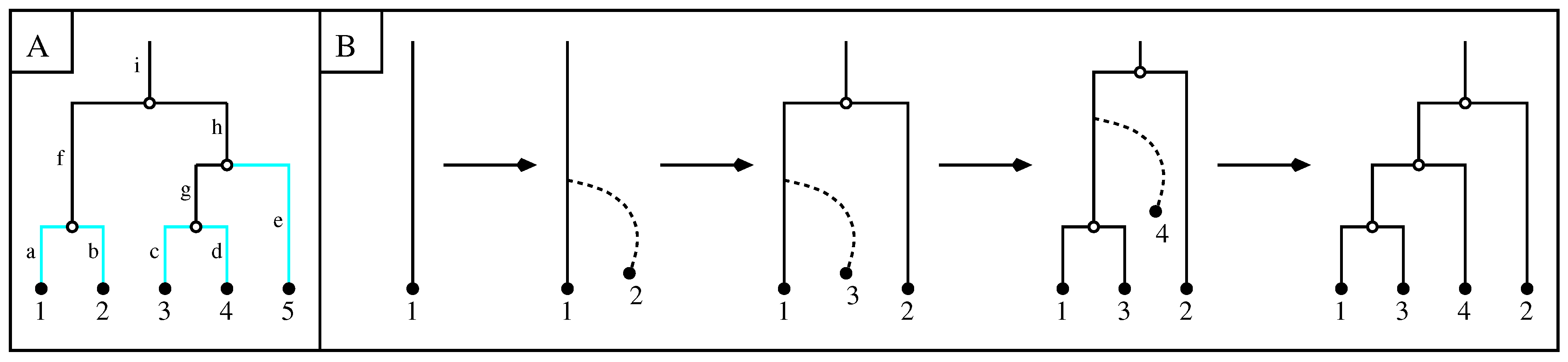
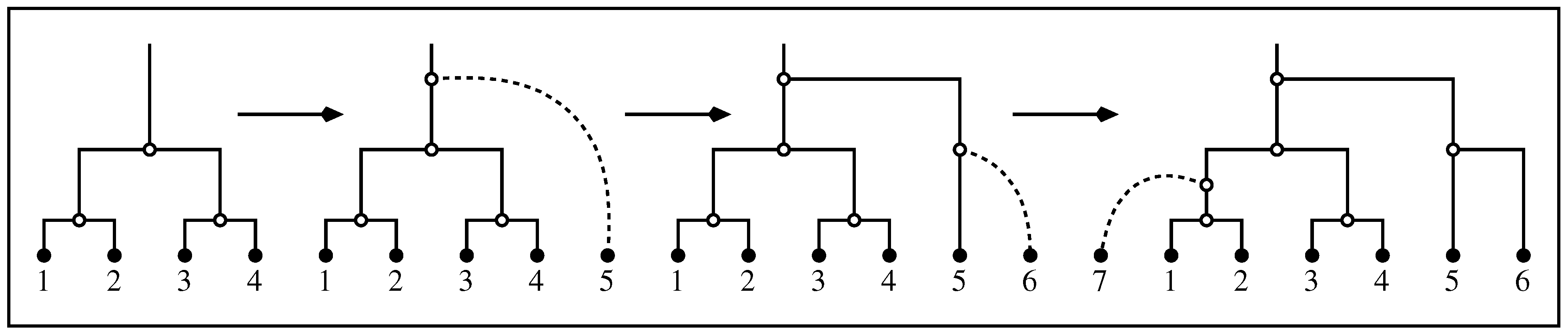
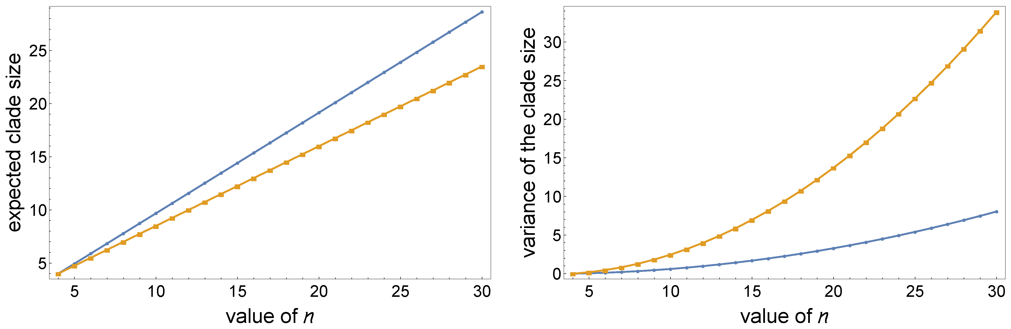
Lower values of the α parameter determine a larger expected clade size and smaller variance. This is shown in Figure 3, where we perform a sequence of α-insertions (2) starting from a labeled topology $t^{\ast }$ of size $k=4$, then calculate the mean and variance of the clade size of the set of leaves $\{1,2,3,4\}$ of $t^{\ast }$ in the resulting random labeled topology of size n (Figure 2).

(iii) 

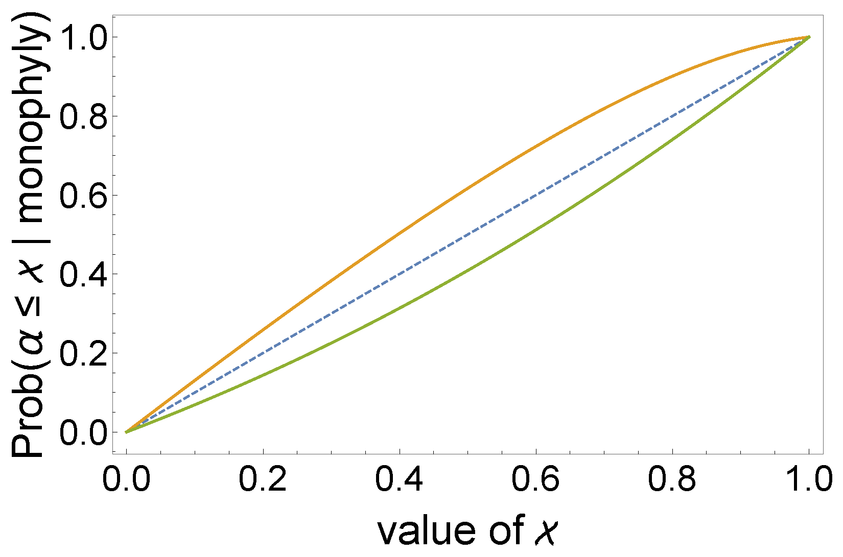
For fixed values of k and d, the asymptotic formula $\Gamma (x+\gamma )\sim \Gamma \left(x\right)x^{\gamma }$ for $x\to +\infty$, which holds for every complex number $\gamma$, yields the following asymptotic expansion as $n\to \infty$ for the probability

$$p_n\left(d\right)\sim {\displaystyle \frac{\Gamma (k-\alpha )\Gamma (d-2\alpha )}{\Gamma \left(\alpha \right)\Gamma (k-2\alpha )\Gamma (d-k+1)}}{\displaystyle \frac{1}{n^{k-2\alpha }}}=\left({\displaystyle \genfrac{}{}{0pt}{}{d-2\alpha -1}{d-k}}\right){\displaystyle \frac{\Gamma (k-\alpha )}{\Gamma \left(\alpha \right)}}{\displaystyle \frac{1}{n^{k-2\alpha }}}.$$

In particular, for increasing values of n, the probability $p_n\left(k\right)$ of the set of initially monophyletic leaves remaining monophyletic decreases to 0 as quickly as $\mathcal{O}(1/n^{k-2\alpha })$. From Theorem 1, the probability $p_n\left(n\right)$ of the clade size of the starting set of leaves being equal to n is instead seen to be $\mathcal{O}(1/n^{\alpha })$. By substituting $d=\rho ·n$ in (4), we find that for $n\to \infty$, the probability of the ratio ${\displaystyle \frac{|\widehat{P}|}{n}}$ being a fixed $\rho <1$ satisfies

$$p_n\left({\displaystyle \frac{|\widehat{P}|}{n}}=\rho \right)\sim {\displaystyle \frac{\Gamma (k-\alpha )}{\Gamma \left(\alpha \right)\Gamma (k-2\alpha )}}·{\displaystyle \frac{1}{n}}{\displaystyle \frac{{\rho }^{k-2\alpha -1}}{{(1-\rho )}^{1-\alpha }}}.$$

(iv) 

It is possible to calculate the probability mass function of the clade size variable without making use of the generalized binomial coefficient. Indeed, by simple algebraic manipulations, from the formula provided in the latter theorem we can also write

$$p_n\left(d\right)={\displaystyle \frac{{\prod }_{j=1}^{n-d}(n-d+\alpha -j){\prod }_{h=1}^{d-k}(d-2\alpha -h)}{{\prod }_{\ell =1}^{n-k}(n-\alpha -\ell )}}\left({\displaystyle \genfrac{}{}{0pt}{}{n-k}{d-k}}\right),$$

where we admit empty products.

4. Probability of Monophyly for a Set of Random Taxa

In this section, we determine the probability ${\mathcal{M}}_n={\mathcal{M}}_n(\alpha ,k)$ that a set P of $k<n$ randomly chosen taxa forms a monophyletic group in a labeled topology of size n selected under the Ford distribution. Without loss of generality, we assume P to be the set of taxa whose labels belong to $\{1,2,\dots ,k\}$ in a random labeled topology of n leaves. Note that when $\alpha =0$, the $\alpha$-model corresponds to the Yule model; from [5], we know that ${\mathcal{M}}_n={\displaystyle \frac{2n}{k(k+1)\left(\genfrac{}{}{0pt}{}{n}{k}\right)}}$. If we instead have $\alpha =1$, then a random labeled topology of size n generated under Ford’s model has a completely unbalanced (caterpillar) tree shape such as the one on the right of Figure 1B. Thus, the probability of the leaves with labels in $P=\{1,2,\dots ,k\}$ forming a monophyletic group is ${\mathcal{M}}_n={\displaystyle \frac{1}{\left(\genfrac{}{}{0pt}{}{n}{k}\right)}}$, as there is only one subtree of size k in such a caterpillar labeled topology.

We now focus on the values of $\alpha$ within the range $0<\alpha <1$. As described in Section 2, a random labeled topology t of n taxa is generated by first selecting a random permutation $\sigma$ of size n, then performing a sequence of random insertions (1). The probability that

$$\sigma =\underset{{\mathit{\sigma }}_0}{\underbrace{{\sigma }_{0,1}\dots {\sigma }_{0,s_0}}}{p}_1\underset{{\mathit{\sigma }}_1}{\underbrace{{\sigma }_{1,1}\dots {\sigma }_{1,s_1}}}{p}_2\underset{{\mathit{\sigma }}_2}{\underbrace{{\sigma }_{2,1}\dots {\sigma }_{2,s_2}}}\dots \underset{{\mathit{\sigma }}_{k-1}}{\underbrace{{\sigma }_{k-1,1}\dots {\sigma }_{k-1,s_{k-1}}}}{p}_k\underset{{\mathit{\sigma }}_k}{\underbrace{{\sigma }_{k,1}\dots {\sigma }_{k,s_k}}},$$

(5)

where each $p_i$ is an element of $\{1,2,\dots ,k\}$ and each ${\mathit{\sigma }}_i$ is a sequence of length $s_i\ge 0$ (with $s_k=n-k-s_0-s_1-\dots -s_{k-1}$) over the alphabet $\{1,2,\dots ,n\}\setminus \{1,2,\dots ,k\}=\{k+1,k+2,\dots ,n\}$, is provided by

$${\displaystyle \frac{k!}{n!}}·\left({\displaystyle \genfrac{}{}{0pt}{}{n-k}{s_0}}\right)s_0!·\left({\displaystyle \genfrac{}{}{0pt}{}{n-k-s_0}{s_1}}\right)s_1!·\dots ·\left({\displaystyle \genfrac{}{}{0pt}{}{n-k-s_0-\dots -s_{k-2}}{s_{k-1}}}\right)s_{k-1}!·s_k!={\displaystyle \frac{1}{\left(\genfrac{}{}{0pt}{}{n}{k}\right)}}.$$

Conditioned on $\sigma$ as in (5), the probability that the set P of taxa is monophyletic after a sequence of random insertions of pendant edges labeled by the symbols in $\sigma$ is a chain of (possibly empty) products

$$\prod _{i=1}^{k-1}a(i+s_0+s_1+\dots +s_i,i)\times \prod _{i=2}^k\prod _{j=0}^{s_i-1}b(i+j+s_0+s_1+\dots +s_{i-1},i),$$

(6)

where $a(z,c)={\displaystyle \frac{c(1-\alpha )}{z-\alpha }}+{\displaystyle \frac{(c-1)\alpha }{z-\alpha }}={\displaystyle \frac{c-\alpha }{z-\alpha }}$ is the probability of attaching a new pendant edge (say, one labeled by x) in a tree of size z that has a clade $\widehat{C}$ of size c, in such a way that the clade size of $\widehat{C\cup \left\{x\right\}}$ is $c+1$ and $b(z,c)={\displaystyle \frac{(z-c)(1-\alpha )}{z-\alpha }}+{\displaystyle \frac{(z-c+1)\alpha }{z-\alpha }}={\displaystyle \frac{z-c+\alpha }{z-\alpha }}$ is the probability of attaching a new pendant edge in a tree of size z that has a clade $\widehat{C}$ of size c, while the clade size of $\widehat{C}$ remains equal to c after the insertion. For instance, if $\widehat{C}$ is the clade $\widehat{C}=((3,4),5)$ of size $c=3$ in the labeled topology t of size $z=5$ depicted in Figure 1A, then a new pendant edge labeled by x can be attached to $c=3$ different pendant edges of t (i.e., $c,d$, and e) or to $c-1=2$ different internal edges of t (i.e., g and h) such that $|\widehat{C\cup \left\{x\right\}}|=c+1=4$, which happens with probability $a(z,c)$. By considering the same tree t of size $z=5$ and the same clade $\widehat{C}=((3,4),5)$ of size $c=3$, we see that a new pendant edge can be attached to $z-c=2$ different pendant edges of t (i.e., a and b) or to $z-c+1=3$ different internal edges of t (i.e., $f,h$, and i) such that after the insertion we have $|\widehat{C}|=c=3$, which happens with probability $b(z,c)$. In particular, each factor $a(i+s_0+s_1+\dots +s_i,i)$ (resp. $b(i+j+s_0+s_1+\dots +s_{i-1},i)$) in (6) yields the probability of the clade size of $\{p_1,\dots ,p_i,p_{i+1}\}$ (resp. $\{p_1,\dots ,p_i\}$) being $i+1$ (resp. i) after insertion of the pending edge labeled by $p_{i+1}$ (resp. ${\sigma }_{i,j+1}$).

Summing over the possible values of $s_0,s_1,\dots ,s_{k-1}$, the probability of the population P of taxa with label in $\{1,2,\dots ,k\}$ being monophyletic in a random labeled topology of size n can then be calculated as follows:

$${\mathcal{M}}_n={\displaystyle \frac{1}{\left(\genfrac{}{}{0pt}{}{n}{k}\right)}}\sum _{s_0=0}^{n-k}\sum _{s_1=0}^{n-k-s_0}\dots \sum _{s_{k-1}=0}^{n-k-s_0-s_1-\dots -s_{k-2}}\prod _{i=1}^{k-1}a(i+s_0+s_1+\dots +s_i,i)\times \prod _{i=2}^k\prod _{j=0}^{s_i-1}b(i+j+s_0+s_1+\dots +s_{i-1},i).$$

(7)

In order to simplify the latter formula for the probability ${\mathcal{M}}_n$, we need the next lemma.

Lemma 2.

Let n be a positive integer; then, we have the following equality for the r nested sums:

$$\sum _{k_1=0}^n\sum _{k_2=0}^{n-k_1}\dots \sum _{k_r=0}^{n-k_1-\dots -k_{r-1}}1=\sum _{0\le k_1\le k_1+k_2\le \dots \le k_1+\dots +k_r\le n}1=\left({\displaystyle \genfrac{}{}{0pt}{}{n+r}{r}}\right).$$

Proof. 

We proceed by induction on $r\ge 1$. If $r=1$, then the sum reduces to $n+1=\left({\displaystyle \genfrac{}{}{0pt}{}{n+1}{1}}\right)$. Now, assuming $r>1$, setting $h=n-k_1+r-1$, and applying the binomial “hockey stick” identity ${\sum }_{x=y}^z\left({\displaystyle \genfrac{}{}{0pt}{}{x}{y}}\right)=\left({\displaystyle \genfrac{}{}{0pt}{}{z+1}{y+1}}\right)$, we obtain

$$\begin{array}{c}\hfill \sum _{k_1=0}^n\sum _{k_2=0}^{n-k_1}\dots \sum _{k_r=0}^{n-k_1-\dots -k_{r-1}}1=\sum _{k_1=0}^n\left({\displaystyle \genfrac{}{}{0pt}{}{n-k_1+r-1}{r-1}}\right)=\sum _{h=r-1}^{n+r-1}\left({\displaystyle \genfrac{}{}{0pt}{}{h}{r-1}}\right)=\left({\displaystyle \genfrac{}{}{0pt}{}{n+r}{r}}\right).\end{array}$$

□

Then, we have the following theorem.

Theorem 2.

Under Ford’s α-model with $0<\alpha <1$, the probability ${\mathcal{M}}_n={\mathcal{M}}_n\left(\alpha \right)$ of the set of leaves $P=\{1,2,\dots ,k\}$ being monophyletic in a random labeled topology of size n is provided by

$${\mathcal{M}}_n={\displaystyle \frac{\left(\genfrac{}{}{0pt}{}{1-2\alpha }{1-\alpha }\right)}{\left(\genfrac{}{}{0pt}{}{n}{k}\right)\left(\genfrac{}{}{0pt}{}{n-1-\alpha }{k-2\alpha }\right)\left(\genfrac{}{}{0pt}{}{k-2\alpha }{1-\alpha }\right)}}\sum _{h=0}^{n-k}(h+1)\left({\displaystyle \genfrac{}{}{0pt}{}{h-\alpha }{1-2\alpha }}\right)\left({\displaystyle \genfrac{}{}{0pt}{}{n-2-h}{k-2}}\right).$$

(8)

Proof. 

We use the following notation: for each $i=0,\dots ,k$, set $z_i=s_0+s_1+\dots +s_i$; then, $s_k=n-k-z_{k-1}$ and $z_k=z_{k-1}+s_k=n-k$. In particular, we can write

$$\begin{array}{cc}& a(i+s_0+s_1+\dots +s_i,i)=a(i+z_i,i)={\displaystyle \frac{i-\alpha }{z_i+i-\alpha }};\hfill \\ & b(i+j+s_0+s_1+\dots +s_{i-1},i)=b(i+j+z_{i-1},i)={\displaystyle \frac{z_{i-1}+j+\alpha }{z_{i-1}+i+j-\alpha }}.\hfill \end{array}$$

Furthermore, for every $z\in \mathbb{C}\setminus {\mathbb{Z}}_{\le 1}$, let $z!=\Gamma (z+1).$

We start by rewriting the products appearing in (7). First, we have

$$\prod _{i=1}^{k-1}a(s_0+s_1+\dots +s_i+i,i)=\prod _{i=1}^{k-1}{\displaystyle \frac{i-\alpha }{z_i+i-\alpha }}={\displaystyle \frac{(k-1-\alpha )!}{(-\alpha )!}}\prod _{i=1}^{k-1}{\displaystyle \frac{1}{z_i+i-\alpha }}.$$

(9)

Second, we find

$$\prod _{j=0}^{s_i-1}b(s_0+s_1+\dots +s_{i-1}+i+j,i)=\prod _{j=0}^{s_i-1}{\displaystyle \frac{z_{i-1}+j+\alpha }{z_{i-1}+i+j-\alpha }}={\displaystyle \frac{(z_i-1+\alpha )!}{(z_{i-1}-1+\alpha )!}}{\displaystyle \frac{(z_{i-1}+i-1-\alpha )!}{(z_i+i-1-\alpha )!}},$$

from which the second product in (7) reads as

$$\begin{array}{ccc}\hfill \prod _{i=2}^k{\displaystyle \frac{(z_i-1+\alpha )!}{(z_{i-1}-1+\alpha )!}}{\displaystyle \frac{(z_{i-1}+i-1-\alpha )!}{(z_i+i-1-\alpha )!}}& =& {\displaystyle \frac{(z_k-1+\alpha )!}{(z_1-1+\alpha )!}}{\displaystyle \frac{(z_1+1-\alpha )!}{(z_k+k-\alpha )!}}\prod _{i=2}^k(z_i+i-\alpha )\hfill \\ & =& {\displaystyle \frac{(n-k-1+\alpha )!}{(n-\alpha -1)!}}{\displaystyle \frac{(z_1-\alpha )!}{(z_1-1+\alpha )!}}\prod _{i=1}^{k-1}(z_i+i-\alpha ).\hfill \end{array}$$

(10)

Hence, by multiplying the products of (9) and (10), we obtain

$$\begin{array}{cc}& {\displaystyle \frac{(n-k-1+\alpha )!}{(n-\alpha -1)!}}{\displaystyle \frac{(z_1-\alpha )!}{(z_1-1+\alpha )!}}{\displaystyle \frac{(k-1-\alpha )!}{(-\alpha )!}}={\displaystyle \frac{\left(\genfrac{}{}{0pt}{}{n-k+\alpha -1}{n-k}\right)}{\left(\genfrac{}{}{0pt}{}{n-1-\alpha }{n-k}\right)}}{\displaystyle \frac{\left(\genfrac{}{}{0pt}{}{z_1-\alpha }{z_1}\right)}{\left(\genfrac{}{}{0pt}{}{z_1+\alpha -1}{z_1}\right)}},\hfill \end{array}$$

and (7) becomes

$${\mathcal{M}}_n={\displaystyle \frac{1}{\left(\genfrac{}{}{0pt}{}{n}{k}\right)}}\sum _{s_0=0}^{n-k}\sum _{s_1=0}^{n-k-s_0}\dots \sum _{s_{k-1}=0}^{n-k-s_0-\dots -s_{k-2}}{\displaystyle \frac{\left(\genfrac{}{}{0pt}{}{n-k+\alpha -1}{n-k}\right)}{\left(\genfrac{}{}{0pt}{}{n-1-\alpha }{n-k}\right)}}{\displaystyle \frac{\left(\genfrac{}{}{0pt}{}{z_1-\alpha }{z_1}\right)}{\left(\genfrac{}{}{0pt}{}{z_1+\alpha -1}{z_1}\right)}}.$$

Because $z_1=s_0+s_1$, we find

$${\mathcal{M}}_n={\displaystyle \frac{\left(\genfrac{}{}{0pt}{}{n-k+\alpha -1}{n-k}\right)}{\left(\genfrac{}{}{0pt}{}{n}{k}\right)\left(\genfrac{}{}{0pt}{}{n-1-\alpha }{n-k}\right)}}\sum _{s_0=0}^{n-k}\sum _{s_1=0}^{n-k-s_0}{\displaystyle \frac{\left(\genfrac{}{}{0pt}{}{z_1-\alpha }{z_1}\right)}{\left(\genfrac{}{}{0pt}{}{z_1+\alpha -1}{z_1}\right)}}\left(\sum _{s_2=0}^{n-k-s_0-s_1}\dots \sum _{s_{k-1}=0}^{n-k-s_0-\dots -s_{k-2}}1\right).$$

From the last lemma, we know that

$$\sum _{s_2=0}^{n-k-s_0-s_1}\dots \sum _{s_{k-1}=0}^{n-k-s_0-\dots -s_{k-2}}1=\left({\displaystyle \genfrac{}{}{0pt}{}{n-k-s_0-s_1+k-2}{k-2}}\right)=\left({\displaystyle \genfrac{}{}{0pt}{}{n-2-z_1}{k-2}}\right).$$

Hence, we obtain

$${\mathcal{M}}_n={\displaystyle \frac{\left(\genfrac{}{}{0pt}{}{n-k+\alpha -1}{n-k}\right)}{\left(\genfrac{}{}{0pt}{}{n}{k}\right)\left(\genfrac{}{}{0pt}{}{n-1-\alpha }{n-k}\right)}}\sum _{s_0=0}^{n-k}\sum _{s_1=0}^{n-k-s_0}{\displaystyle \frac{\left(\genfrac{}{}{0pt}{}{z_1-\alpha }{z_1}\right)}{\left(\genfrac{}{}{0pt}{}{z_1+\alpha -1}{z_1}\right)}}\left({\displaystyle \genfrac{}{}{0pt}{}{n-2-z_1}{k-2}}\right).$$

Setting $h=z_1=s_0+s_1$ and denoting the argument of the latter sum by $f\left(h\right)$, we have

$$\sum _{s_0=0}^{n-k}\sum _{s_1=0}^{n-k-s_0}f\left(h\right)=\sum _{h=0}^{n-k}(h+1)f\left(h\right),$$

where

$$(h+1)f\left(h\right)={\displaystyle \frac{(h+1)\left(\genfrac{}{}{0pt}{}{h-\alpha }{h}\right)}{\left(\genfrac{}{}{0pt}{}{h+\alpha -1}{h}\right)}}\left({\displaystyle \genfrac{}{}{0pt}{}{n-2-h}{k-2}}\right)=(\alpha -1){\displaystyle \frac{\left(\genfrac{}{}{0pt}{}{h-\alpha }{h}\right)}{\left(\genfrac{}{}{0pt}{}{h+\alpha -1}{h+1}\right)}}\left({\displaystyle \genfrac{}{}{0pt}{}{n-2-h}{k-2}}\right).$$

Thus, the formula for ${\mathcal{M}}_n$ can be written as

$$\begin{array}{ccc}\hfill {\mathcal{M}}_n& =& {\displaystyle \frac{\left(\genfrac{}{}{0pt}{}{n-k+\alpha -1}{n-k}\right)}{\left(\genfrac{}{}{0pt}{}{n}{k}\right)\left(\genfrac{}{}{0pt}{}{n-1-\alpha }{n-k}\right)}}(\alpha -1)\sum _{h=0}^{n-k}{\displaystyle \frac{\left(\genfrac{}{}{0pt}{}{h-\alpha }{h}\right)}{\left(\genfrac{}{}{0pt}{}{h+\alpha -1}{h+1}\right)}}\left({\displaystyle \genfrac{}{}{0pt}{}{n-2-h}{k-2}}\right)\hfill \\ & =& {\displaystyle \frac{\left(\genfrac{}{}{0pt}{}{1-2\alpha }{1-\alpha }\right)}{\left(\genfrac{}{}{0pt}{}{n}{k}\right)\left(\genfrac{}{}{0pt}{}{n-1-\alpha }{k-2\alpha }\right)\left(\genfrac{}{}{0pt}{}{k-2\alpha }{1-\alpha }\right)}}\sum _{h=0}^{n-k}(h+1)\left({\displaystyle \genfrac{}{}{0pt}{}{h-\alpha }{1-2\alpha }}\right)\left({\displaystyle \genfrac{}{}{0pt}{}{n-2-h}{k-2}}\right),\hfill \end{array}$$

where in the second identity we have used the fact that

$$\begin{array}{ccc}\hfill (\alpha -1){\displaystyle \frac{\left(\genfrac{}{}{0pt}{}{h-\alpha }{h}\right)}{\left(\genfrac{}{}{0pt}{}{h+\alpha -1}{h+1}\right)}}& =& (\alpha -1){\displaystyle \frac{(h-\alpha )!(h+1)!(\alpha -2)!}{h!(-\alpha )!(h+\alpha -1)!}}={\displaystyle \frac{h+1}{\left(\genfrac{}{}{0pt}{}{-\alpha }{1-2\alpha }\right)}}\left({\displaystyle \genfrac{}{}{0pt}{}{h-\alpha }{1-2\alpha }}\right).\hfill \end{array}$$

□

Remark 2.

From the latter theorem, we observe the following.

(i) 

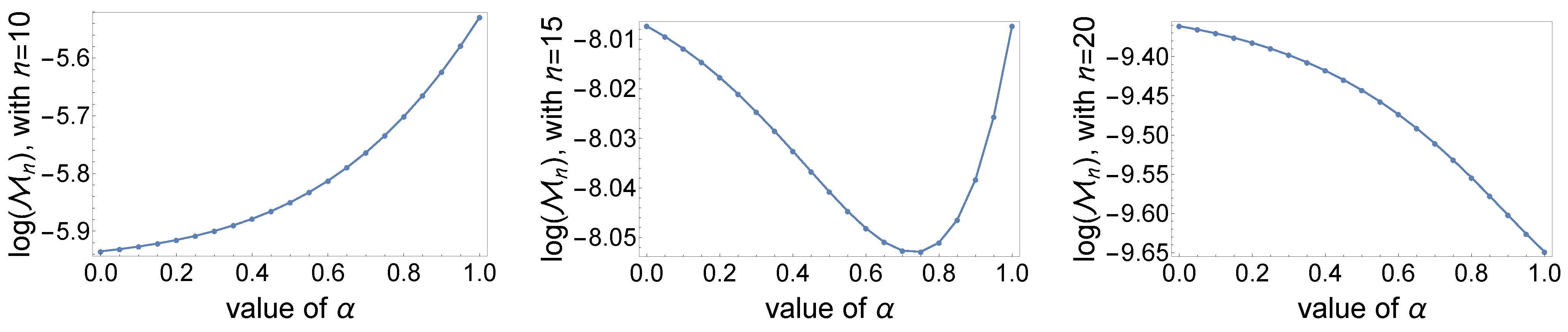
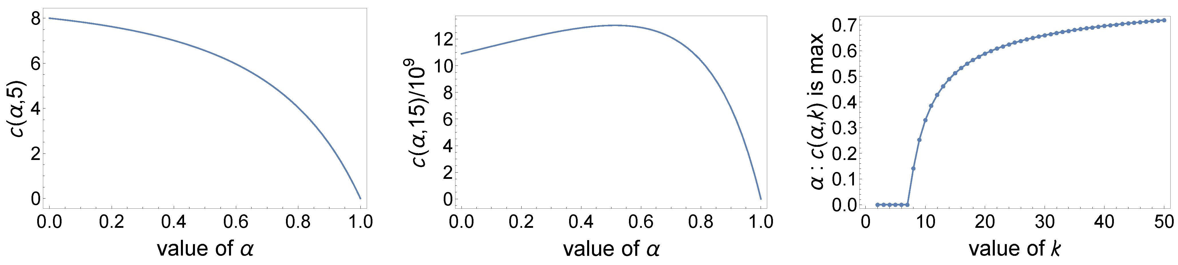
For different values of n, we can observe a different behavior by plotting the (natural logarithm of the) probability ${\mathcal{M}}_n$ as a function of α (Figure 4). The mentioned probability can be an increasing function of α (left panel), a decreasing function of α (right panel), or a unimodal function of α (middle panel).

(ii) 

The formula for ${\mathcal{M}}_n$ that appears in (8) calculates the probability of monophyly for a set of k taxa chosen at random from among the leaves of a labeled topology of size n selected under the Ford’s distribution and when $\alpha =0$ or $\alpha =1$ (the latter when we consider the limit $\alpha \to 1^{-}$). Indeed, for $\alpha =0$, by substituting $j=h+1$ in the third of the following equalities and applying the Chu–Vandermonde identity in the fourth equality, the formula for ${\mathcal{M}}_n={\mathcal{M}}_n(\alpha ,k)$ reduces to

$$\begin{array}{ccc}\hfill {\mathcal{M}}_n(0,k)& =& {\left.{\displaystyle \frac{\left(\genfrac{}{}{0pt}{}{1-2\alpha }{1-\alpha }\right)}{\left(\genfrac{}{}{0pt}{}{n}{k}\right)\left(\genfrac{}{}{0pt}{}{n-1-\alpha }{k-2\alpha }\right)\left(\genfrac{}{}{0pt}{}{k-2\alpha }{1-\alpha }\right)}}\sum _{h=0}^{n-k}(h+1)\left({\displaystyle \genfrac{}{}{0pt}{}{h-\alpha }{1-2\alpha }}\right)\left({\displaystyle \genfrac{}{}{0pt}{}{n-2-h}{k-2}}\right)\right|}_{\alpha =0}\hfill \\ & =& {\displaystyle \frac{1}{\left(\genfrac{}{}{0pt}{}{n}{k}\right)\left(\genfrac{}{}{0pt}{}{n-1}{k}\right)k}}\sum _{h=0}^{n-2}(h+1)h\left({\displaystyle \genfrac{}{}{0pt}{}{n-2-h}{k-2}}\right)\hfill \\ & =& {\displaystyle \frac{2}{\left(\genfrac{}{}{0pt}{}{n}{k}\right)\left(\genfrac{}{}{0pt}{}{n-1}{k}\right)k}}\sum _{j=0}^{n-1}\left({\displaystyle \genfrac{}{}{0pt}{}{j}{2}}\right)\left({\displaystyle \genfrac{}{}{0pt}{}{n-1-j}{k-2}}\right)\hfill \\ & =& {\displaystyle \frac{2}{\left(\genfrac{}{}{0pt}{}{n}{k}\right)\left(\genfrac{}{}{0pt}{}{n-1}{k}\right)k}}\left({\displaystyle \genfrac{}{}{0pt}{}{n}{k+1}}\right)\hfill \\ & =& {\displaystyle \frac{2n}{k(k+1)\left(\genfrac{}{}{0pt}{}{n}{k}\right)}}.\hfill \end{array}$$

Furthermore, when $\alpha \to 1^{-}$, we can use Legendre’s duplication formula to find

$$\begin{array}{cc}\hfill & \underset{\alpha \to 1^{-}}{lim}\left({\displaystyle \genfrac{}{}{0pt}{}{1-2\alpha }{1-\alpha }}\right)=\underset{\alpha \to 1^{-}}{lim}{\displaystyle \frac{\Gamma (2-2\alpha )}{\Gamma (2-\alpha )\Gamma (1-\alpha )}}=\underset{\alpha \to 1^{-}}{lim}{\displaystyle \frac{1}{2^{1-2(1-\alpha )}\sqrt{\pi }}}\Gamma \left(1-\alpha +{\displaystyle \frac{1}{2}}\right)={\displaystyle \frac{1}{2}}.\hfill \end{array}$$

For $h=1,\dots ,n-k$, we have

$$\begin{array}{c}\underset{\alpha \to 1^{-}}{lim}\left({\displaystyle \genfrac{}{}{0pt}{}{h-\alpha }{1-2\alpha }}\right)=\underset{\alpha \to 1^{-}}{lim}{\displaystyle \frac{\Gamma (h+1-\alpha )}{\Gamma (2-2\alpha )\Gamma (h+\alpha )}}=\underset{\alpha \to 1^{-}}{lim}{\displaystyle \frac{\Gamma \left(h\right)}{\Gamma (2-2\alpha )\Gamma (h+1)}}=0,\hfill \end{array}$$

while $h=0$ provides

$$\begin{array}{c}\underset{\alpha \to 1^{-}}{lim}\left({\displaystyle \genfrac{}{}{0pt}{}{-\alpha }{1-2\alpha }}\right)=\underset{\alpha \to 1^{-}}{lim}{\displaystyle \frac{\Gamma (1-\alpha )}{\Gamma (2-2\alpha )\Gamma \left(\alpha \right)}}=\underset{\alpha \to 1^{-}}{lim}{\displaystyle \frac{\Gamma (1-\alpha )}{\Gamma (2-2\alpha )}}=2.\hfill \end{array}$$

Hence,

$$\underset{\alpha \to 1^{-}}{lim}{\mathcal{M}}_n(\alpha ,k)={\displaystyle \frac{1/2}{\left(\genfrac{}{}{0pt}{}{n}{k}\right)\left(\genfrac{}{}{0pt}{}{n-2}{k-2}\right)}}2\left({\displaystyle \genfrac{}{}{0pt}{}{n-2}{k-2}}\right)={\displaystyle \frac{1}{\left(\genfrac{}{}{0pt}{}{n}{k}\right)}},$$

showing that the formula in (8) extended by continuity to $\alpha =1$ yields the right expression for the probability ${\mathcal{M}}_n$.

(iii) 

The formula for ${\mathcal{M}}_n$ provided in the latter theorem can be further simplified for fixed values of k. For instance, when $k=2$ or $k=3$, Equation (8) respectively reduces to the following:

$${\mathcal{M}}_n={\displaystyle \frac{\Gamma (n-\alpha )\Gamma (\alpha -2)(\alpha +(2-2\alpha \left)n\right)+\Gamma (1-\alpha )\Gamma (n-2+\alpha )}{2(3-2\alpha )\Gamma (n-\alpha )\Gamma (\alpha -2)\left(\genfrac{}{}{0pt}{}{n}{2}\right)}}$$

and

$${\mathcal{M}}_n={\displaystyle \frac{\left(\right(1-\alpha )n+\alpha )\Gamma (n-\alpha )\Gamma (\alpha -2)+\left(\right(2-\alpha )n+\alpha -3)\Gamma (1-\alpha )\Gamma (n-3+\alpha )}{2(3-2\alpha )\Gamma (n-\alpha )\Gamma (\alpha -2)\left(\genfrac{}{}{0pt}{}{n}{3}\right)}}.$$

More generally, explicit expressions for ${\mathcal{M}}_n$ can be determined for fixed values of k by writing the sum in (8) as a telescoping sum:

$$\sum _{h=0}^{n-k}(h+1)\left({\displaystyle \genfrac{}{}{0pt}{}{h-\alpha }{1-2\alpha }}\right)\left({\displaystyle \genfrac{}{}{0pt}{}{n-2-h}{k-2}}\right)=\sum _{h=0}^{n-k}g(h+1)-g\left(h\right)=g(n-k+1)-g\left(0\right)$$

(11)

where

$$g\left(h\right)=(2-2\alpha )A\left(h\right)\left({\displaystyle \genfrac{}{}{0pt}{}{h-\alpha }{2-2\alpha }}\right)$$

for a polynomial $A\left(h\right)=a_{k-1}{h}^{k-1}+a_{k-2}{h}^{k-2}+\dots +a_0$ whose coefficients satisfy

$$a_{k-1}={\displaystyle \frac{{(-1)}^{k-2}}{(k+1-2\alpha )(k-2)!}}$$

(12)

and the linear system

$$\left\{\begin{array}{cc}A\left(0\right)={\displaystyle \frac{2-\alpha }{\alpha }}A(-1)\hfill & \\ A(n-k+i+1)={\displaystyle \frac{n-k+i+\alpha -1}{n-k+i+1-\alpha }}A(n-k+i),\hfill & i=1,\dots ,k-2.\hfill \end{array}\right.$$

(13)

Note that if $A\left(h\right)$ satisfies (12) and (13), then as in the first equality of (11) we indeed find

$$\begin{array}{ccc}\hfill g(h+1)-g\left(h\right)& =& (2-2\alpha )\left[A(h+1)\left({\displaystyle \genfrac{}{}{0pt}{}{h+1-\alpha }{2-2\alpha }}\right)-A\left(h\right)\left({\displaystyle \genfrac{}{}{0pt}{}{h-\alpha }{2-2\alpha }}\right)\right]\hfill \\ & =& \left({\displaystyle \genfrac{}{}{0pt}{}{h-\alpha }{1-2\alpha }}\right)·\left(A(h+1)(h+1-\alpha )-A\left(h\right)(h+\alpha -1)\right)\hfill \\ & =& \left({\displaystyle \genfrac{}{}{0pt}{}{h-\alpha }{1-2\alpha }}\right)·(h+1)\left({\displaystyle \genfrac{}{}{0pt}{}{n-2-h}{k-2}}\right),\hfill \end{array}$$

because $A(h+1)(h+1-\alpha )-A\left(h\right)(h+\alpha -1)$ and $(h+1)\left({\displaystyle \genfrac{}{}{0pt}{}{n-2-h}{k-2}}\right)=(h+1)$${\displaystyle \frac{(n-2-h)·\dots ·(n-k-h+1)}{(k-2)!}}$ are identical as polynomials of degree $k-1$ in the variable h with leading coefficient ${(-1)}^{k-2}/(k-2)!$ and roots $-1,n-k+1,n-k+2,\dots ,n-3,n-2$.

We conclude this section with an asymptotic estimate for ${\mathcal{M}}_n$ when $\alpha$ and k are fixed and n goes to infinity.

Theorem 3.

Fix $0<\alpha <1$ and $k\ge 2$; then, when $n\to \infty$, we have the following asymptotic equivalence:

$${\mathcal{M}}_n\sim {\displaystyle \frac{\left(\genfrac{}{}{0pt}{}{2-2\alpha }{2-\alpha }\right)}{\left(\genfrac{}{}{0pt}{}{k+1-2\alpha }{2-\alpha }\right)}}{\displaystyle \frac{k!}{n^{k-1}}}.$$

Proof. 

We start by analyzing the sum

$$\sum _{h=0}^{n-k}(h+1)\left({\displaystyle \genfrac{}{}{0pt}{}{h-\alpha }{1-2\alpha }}\right)\left({\displaystyle \genfrac{}{}{0pt}{}{n-h-2}{k-2}}\right)={\displaystyle \frac{1}{\Gamma (2-2\alpha )(k-2)!}}\sum _{h=0}^{n-k}\phi \left(h\right),$$

where

$$\phi \left(h\right)=\Gamma (2-2\alpha )(k-2)!·(h+1)\left({\displaystyle \genfrac{}{}{0pt}{}{h-\alpha }{1-2\alpha }}\right)\left({\displaystyle \genfrac{}{}{0pt}{}{n-h-2}{k-2}}\right).$$

We write

$$\left({\displaystyle \genfrac{}{}{0pt}{}{h-\alpha }{1-2\alpha }}\right)={\displaystyle \frac{1}{\Gamma (2-2\alpha )}}{\displaystyle \frac{\Gamma (h+1-\alpha )}{\Gamma (h+\alpha )}}={\displaystyle \frac{1}{\Gamma (2-2\alpha )}}{\displaystyle \frac{\Gamma (h+1-\alpha )}{\Gamma (h+1)}}{\displaystyle \frac{\Gamma (h+1)}{\Gamma (h+\alpha )}}.$$

For $h\ge 1$, Gautschi’s inequality (which states that $x^{1-s}<\Gamma (x+1)/\Gamma (x+s)<{(x+1)}^{1-s}$ for every positive real number x and every s in $(0,1)$) yields

$${\displaystyle \frac{h^{1-\alpha }{(h+1)}^{-\alpha }}{\Gamma (2-2\alpha )}}<\left({\displaystyle \genfrac{}{}{0pt}{}{h-\alpha }{1-2\alpha }}\right)<{\displaystyle \frac{{(h+1)}^{1-\alpha }{h}^{-\alpha }}{\Gamma (2-2\alpha )}}.$$

Combining this with the elementary inequality

$${\displaystyle \frac{{(n-h-k+1)}^{k-2}}{(k-2)!}}<\left({\displaystyle \genfrac{}{}{0pt}{}{n-h-2}{k-2}}\right)<{\displaystyle \frac{{(n-h-2)}^{k-2}}{(k-2)!}},$$

we obtain

$$L\left(n\right)\equiv \sum _{h=1}^{n-k}{\left(h(h+1)\right)}^{1-\alpha }{(n-h-k+1)}^{k-2}<\sum _{h=1}^{n-k}\phi \left(h\right)<\sum _{h=1}^{n-k}{(h+1)}^{2-\alpha }{h}^{-\alpha }{(n-h-2)}^{k-2}\equiv U\left(n\right),$$

where we have used $L\left(n\right)$ and $U\left(n\right)$ to respectively denote the lower and upper bounds of the previous inequality. For $m\ge 1$, $a>0$ and $b\ge 0$, consider the function $f:[0,m]\to [0,\infty )$ defined by $f\left(t\right)=t^a{(m-t)}^b$ (with the convention $0^0=1$). Note that f is (strictly) increasing for $0<t<t_0={\displaystyle \frac{am}{a+b}}$, (strictly) decreasing for $t_0\le t\le m$, and admits a maximum $f\left(t_0\right)=C_{a,b}{m}^{a+b}$ with $C_{a,b}=a^a{b}^b{(a+b)}^{-(a+b)}$. Note also that by the substitution $t=mu$ we have

$${\int }_0^{m}f\left(t\right)\mathrm{d}t=m^{a+b+1}{\int }_0^1{u}^a{(1-u)}^b\mathrm{d}u=m^{a+b+1}B(a+1,b+1),$$

where $B(z,w)=\Gamma \left(z\right)\Gamma \left(w\right)/\Gamma (z+w)$ is the Beta function defined for every complex number z and w such that $\Re \left(z\right)>0$ and $\Re \left(w\right)>0$. Because

$$\sum _{h=1}^{m}f\left(h\right)=\sum _{h=0}^{\lfloor t_0\rfloor }f\left(h\right)+f(\lfloor t_0\rfloor +1)+\sum _{h=\lfloor t_0\rfloor +2}^{m}f\left(h\right)\le {\int }_0^{m}f\left(t\right)\mathrm{d}t+f(\lfloor t_0\rfloor +1)\le {\int }_0^{m}f\left(t\right)\mathrm{d}t+f\left(t_0\right)$$

and

$$\sum _{h=1}^{m}f\left(h\right)+f\left(t_0\right)=\sum _{h=0}^{m}f\left(h\right)+f\left(t_0\right)\ge {\int }_0^{m}f\left(t\right)\mathrm{d}t,$$

we find

$$\begin{array}{cc}\hfill -f\left(t_0\right)+{\int }_0^{m}f\left(t\right)\mathrm{d}t& \le \sum _{h=1}^{m}f\left(h\right)\le f\left(t_0\right)+{\int }_0^{m}f\left(t\right)\mathrm{d}t,\hfill \end{array}$$

that is,

$$\begin{array}{cc}\hfill -C_{a,b}{m}^{a+b}+m^{a+b+1}B(a+1,b+1)& \le \sum _{h=1}^{m}f\left(h\right)\le C_{a,b}{m}^{a+b}+m^{a+b+1}B(a+1,b+1).\hfill \end{array}$$

We apply the latter estimates to bound $L\left(n\right)$ and $U\left(n\right)$. For each $a>0$, we denote $C_a=C_{a,k-2}$. We first consider $L\left(n\right)$. Because $1-\alpha >0$, we have

$$\begin{array}{cc}\hfill L\left(n\right)& >\sum _{h=1}^{n-k}{h}^{2-2\alpha }{(n-k-h)}^{k-2}\ge -C_{2-2\alpha }{(n-k)}^{k-2\alpha }+{(n-k)}^{k+1-2\alpha }B(3-2\alpha ,k-1).\hfill \end{array}$$

We now focus on $U\left(n\right)$. Since ${(h+1)}^2\le h^2+3h$ and $h^{-2\alpha }\le h^{-\alpha }$, we have

$$\begin{array}{cc}\hfill U\left(n\right)& =\sum _{h=1}^{n-k}{(h+1)}^{2-\alpha }{h}^{-\alpha }{(n-h-2)}^{k-2}<\sum _{h=1}^n{(h+1)}^2{h}^{-2\alpha }{(n-h)}^{k-2}\hfill \\ \hfill & <\sum _{h=1}^n{h}^{2-2\alpha }{(n-h)}^{k-2}+3\sum _{h=1}^n{h}^{1-\alpha }{(n-h)}^{k-2}\hfill \\ \hfill & \le C_{2-2\alpha }{n}^{k-2\alpha }+n^{k+1-2\alpha }B(3-2\alpha ,k-1)+3C_{1-\alpha }{n}^{k-\alpha -1}+3B(2-\alpha ,k-1)n^{k-\alpha }.\hfill \end{array}$$

Thus, both $L\left(n\right)$ and $U\left(n\right)$ are asymptotically equivalent to $B(3-2\alpha ,k-1)n^{k+1-2\alpha }$, as $n\to \infty$; therefore, so is ${\sum }_{h=1}^{n-k}\phi \left(h\right)$. Because $\phi \left(0\right)=o\left(n^{k+1-2\alpha }\right)$, we can conclude that

$$\begin{array}{c}\hfill \sum _{h=0}^{n-k}(h+1)\left({\displaystyle \genfrac{}{}{0pt}{}{h-\alpha }{1-2\alpha }}\right)\left({\displaystyle \genfrac{}{}{0pt}{}{n-h-2}{k-2}}\right)\sim {\displaystyle \frac{B(3-2\alpha ,k-1)}{\Gamma (2-2\alpha )(k-2)!}}{n}^{k+1-2\alpha }={\displaystyle \frac{2-2\alpha }{\Gamma (k+2-2\alpha )}}{n}^{k+1-2\alpha }.\end{array}$$

Finally, by inserting the latter formula into (8) together with the asymptotic equivalences

$$\left({\displaystyle \genfrac{}{}{0pt}{}{n}{k}}\right)\sim {\displaystyle \frac{n^k}{k!}}\mathrm{and}\left({\displaystyle \genfrac{}{}{0pt}{}{n-1-\alpha }{k-2\alpha }}\right)\sim {\displaystyle \frac{n^{k-2\alpha }}{\Gamma (k+1-2\alpha )}},$$

we find

$$\begin{array}{cc}\hfill {\mathcal{M}}_n& \sim {\displaystyle \frac{\left(\genfrac{}{}{0pt}{}{1-2\alpha }{1-\alpha }\right)}{\left(\genfrac{}{}{0pt}{}{k-2\alpha }{1-\alpha }\right)}}{\displaystyle \frac{\Gamma (k+1-2\alpha )k!}{n^{2k-2\alpha }}}{\displaystyle \frac{2-2\alpha }{\Gamma (k+2-2\alpha )}}{n}^{k+1-2\alpha }={\displaystyle \frac{\left(\genfrac{}{}{0pt}{}{2-2\alpha }{2-\alpha }\right)}{\left(\genfrac{}{}{0pt}{}{k+1-2\alpha }{2-\alpha }\right)}}{\displaystyle \frac{k!}{n^{k-1}}}.\hfill \end{array}$$

□

From Theorem 3 and the formulas for ${\mathcal{M}}_n$ provided at the beginning of this section for $\alpha =0$ and $\alpha =1$, we find that ${\mathcal{M}}_n$ behaves as follows for $n\to \infty$:

$${\mathcal{M}}_n\sim \left\{\begin{array}{cc}c(\alpha ,k)·n^{1-k},\hfill & \mathrm{if}0\le \alpha <1\hfill \\ k!·n^{-k},\hfill & \mathrm{if}\alpha =1\hfill \end{array}\right.$$

(14)

where $c(\alpha ,k)={\displaystyle \frac{k!\left(\genfrac{}{}{0pt}{}{2-2\alpha }{2-\alpha }\right)}{\left(\genfrac{}{}{0pt}{}{k+1-2\alpha }{2-\alpha }\right)}}$.

The asymptotic constant $c(\alpha ,k)$ is plotted in Figure 5 for $k=5$ (left) and $k=15$ (center). The plot has different shapes depending on k; it is strictly decreasing when $k=5$, while it has a maximum at $\alpha \approx 0.5$ when $k=15$. The value of the parameter $\alpha$ at which the constant $c(\alpha ,k)$ reaches its maximum is shown as a function of $k\in [2,50]$ on the right of Figure 5. Note that for small values of k, i.e., $k\le 7$, $c(\alpha ,k)$ is maximum when $\alpha =0$, that is, when the Ford model corresponds to the Yule model. When $k\approx 15$, the uniform model ($\alpha \approx 1/2$) is the phylogenetic scenario that maximizes $c(\alpha ,k)$.

5. Conclusions

In this article, we have investigated the distributive properties of the clade size $|\widehat{P}|$ of a population P of k leaves taken from n taxa of a labeled topology generated at random under different scenarios in the framework of Ford’s $\alpha$-model.

Our goal in Section 3 was to measure how much a sequence of random $\alpha$-insertions modifies the clade size of a set of initially monophyletic leaves. To this end, in Theorem 1 we have determined the probability mass function, mean, and variance of the clade size of the set $P=\{1,2,\dots ,k\}$ of k leaves belonging to a random labeled topology of size $n\ge k$ obtained through a sequence of $n-k$$\alpha$-insertions starting from a tree of size k labeled by the symbols in P. As might be expected, our results show that lowering the value of the parameter $\alpha$, that is, decreasing the probability of attaching new leaves at the internal edges of the tree, increases the expectation of the clade size variable and reduces its variance (Figure 3).

Next, Section 4 was dedicated to the study of monophyly under the $\alpha$-model. In Theorem 2, we have derived a formula for calculating the probability ${\mathcal{M}}_n={\mathcal{M}}_n(\alpha ,k)$ that a set of k randomly chosen taxa is monophyletic in a labeled topology of size $n\ge k$ selected under the Ford distribution with parameter $\alpha$. Previous studies [3,4] have investigated the probability of monophyly for the special cases of $\alpha =0$ and $\alpha =1/2$, respectively corresponding to the Yule and uniform distributions of labeled topologies of a given size. Our formula for ${\mathcal{M}}_n$ allows for the inference of the parameter $\alpha$ by conditioning on the monophyly of a random sample of k leaves in a labeled topology of size n generated under the Ford model. In particular, the conditional density function of $\alpha$ reads as

$$f_{\alpha |\mathrm{monophyly}}\left(x\right)={\displaystyle \frac{\mathrm{Prob}\left(\mathrm{monophyly}\right|\alpha =x)·f_{\alpha }\left(x\right)}{{\int }_0^1\mathrm{Prob}\left(\mathrm{monophyly}\right|\alpha =u)·f_{\alpha }\left(u\right)du}}={\displaystyle \frac{{\mathcal{M}}_n(x,k)·f_{\alpha }\left(x\right)}{{\int }_0^1{\mathcal{M}}_n(u,k)·f_{\alpha }\left(u\right)du}},$$

where $f_{\alpha }\left(x\right)$ is the prior density function of $\alpha$. In Figure 6, assuming a uniform prior distribution on the $\alpha$ parameter, i.e., $f_{\alpha }\left(x\right)=1$, we plot the conditional cumulative distribution of $\alpha$ when a random sample of k leaves is observed to be monophyletic in a random labeled topology of size $n=100$. The plot shows that for a relatively small value of k, i.e., $k=5$ (top curve), the probability of $\alpha \le x$ is increased for every x with respect to the prior distribution (the dashed line). For a larger value of k, i.e., $k=20$ (bottom curve), the probability of $\alpha \ge x$ instead increases for every x, suggesting that small values of alpha are more likely when observing the monophyly of a small sample of leaves. This is confirmed by the plot in Figure 7, where we have calculated the conditional probability of $\alpha$ being either small ($\alpha \le 0.2$), medium ($0.4\le \alpha \le 0.6$) or large ($\alpha \ge 0.8$) when k random leaves are seen to be monophyletic in a Ford-distributed tree of size $n=100$, again assuming a uniform prior distribution on $\alpha$. The probability of a small or large value of $\alpha$ respectively decreases or increases with the first values of k, while the probability of a medium value of $\alpha$ appears to be more uncorrelated with k. For small, medium, or large $\alpha$, the Ford model has its best-known instances respectively provided by the Yule ($\alpha =0$), uniform ($\alpha =1/2$), or comb ($\alpha =1$) model of random labeled topologies, respectively, and our calculations can be used to infer which model is more likely to produce a given tree of size n in which a set of k random leaves is found to form a clade. In the final part of Section 4, we have further investigated the probability of monophyly ${\mathcal{M}}_n$ by determining its asymptotic behavior (Theorem 3). We have shown that ${\mathcal{M}}_n$ decreases like a constant multiple of $n^{1-k}$ for every $0\le \alpha <1$, that is, ${\mathcal{M}}_n\sim c(\alpha ,k)·n^{1-k}$ as in (14). Thus, for a given value of k, the probability of monophyly is asymptotically larger for those values of $\alpha$ at which the factor $c(\alpha ,k)$ attains its maximum (Figure 5, right).

Our investigation of the probability of monophyly also relates to other studies of leaf-induced subtrees. In [9], for a uniformly distributed labeled topology T of size n, the authors studied in the limit $n\to \infty$ the maximum value of the probability $\gamma (B,T)$ of observing a fixed “caterpillar” or “even” tree B of size k as the clade of a set of k leaves randomly sampled in T. The probability of monophyly studied in the latter section of the present paper for a Ford-distributed labeled topology T of size n can be seen as the sum of the quantities $\gamma (B,T)$, when all trees B of k leaves are considered.

Several directions of research naturally arise from this work. In Section 4, our focus has been on the probability of the clade size of a set of k random taxa in a Ford distributed labeled topology of given size being equal to k. It would be of interest to extend our calculations to broaden the results of [5] by determining the entire distribution of the clade size variable of a set of k randomly chosen taxa in a labeled topology of size n sampled under the Ford distribution. We remark that the population P for which the clade size is studied in Section 3 is not a set of k randomly chosen taxa of a random labeled topology t of size n, as P corresponds to the set of leaves present in the labeled topology $t^{\ast }$ from which a sequence of $\alpha$-insertions has produced t. It also remains to investigate reciprocal monophyly, that is, the probability of two (or more) prespecified groups of leaves being monophyletic in a random tree selected under Ford’s distribution. This probability was calculated for $\alpha =0$ in Theorem 4.5 of [3]; however, a generalization to arbitrary values of $\alpha$ remains missing.

References

1. Aldous, D.J. Stochastic models and descriptive statistics for phylogenetic trees, from Yule to today. Stat. Sci. 2001, 16, 23–34. [Google Scholar] [CrossRef]
2. Ford, D.J. Probabilities on cladograms: Introduction to the alpha model. arXiv 2005, arXiv:0511246. [Google Scholar]
3. Zhu, S.; Degnan, J.H.; Steel, M. Clades, clans, and reciprocal monophyly under neutral evolutionary models. Theor. Popul. Biol. 2011, 79, 220–227. [Google Scholar] [CrossRef] [PubMed]
4. Zhu, S.; Than, C.; Wu, T. Clades and clans: A comparison study of two evolutionary models. J. Math. Biol. 2015, 71, 99–124. [Google Scholar] [CrossRef] [PubMed]
5. Di Nunzio, A.; Disanto, F. Clade size distribution under neutral evolutionary models. Theor. Popul. Biol. 2024, 156, 93–102. [Google Scholar] [CrossRef]
6. Rosenberg, N.A. The mean and variance of the numbers of r-pronged nodes and r-caterpillars in Yule-generated genealogical trees. Ann. Comb. 2006, 10, 129–146. [Google Scholar] [CrossRef]
7. Semple, C.; Steel, M. Phylogenetics; Oxford Univ. Press: Oxford, UK, 2003. [Google Scholar]
8. Coronado, T.M.; Mir, A.; Rosselló, F. The probabilities of trees and cladograms under Ford’s α-model. Sci. World J. 2018, 2018, 1916094. [Google Scholar] [CrossRef] [PubMed]
9. Czabarka, E.; Székely, L.A.; Wagner, S. Inducibility in Binary Trees and Crossings in Random Tanglegrams. SIAM J. Discret. Math. 2017, 31, 1732–1750. [Google Scholar] [CrossRef]
Figure 1. Labeled topologies and a sequence of α -insertions. (A) A labeled topology of size n = 5. The tree has n = 5 pendant edges (those in gray, denoted by the letters a , b , c , d , and e) and n 1 = 4 internal edges (those in black, denoted by the letters f , g , h , and i). (B) The labeled topology ( ( ( 1 , 3 ) , 4 ) , 2 ) on the right generated under the α -model, when σ = σ 1 σ 2 σ 3 σ 4 = 1234 , is the permutation that determines the label σ i of the pendant edge added with the i-th insertion in (1).
Mathematics 12 03974 g001
Figure 2. A sequence of α -insertions. Starting from the labeled topology t = ( ( 1 , 2 ) , ( 3 , 4 ) ) depicted on the left, the sequence generates the labeled topology t of size 7 depicted on the right. After the insertions, the clade size of the set of leaves P = { 1 , 2 , 3 , 4 } inherited from t has increased by one, as P ^ = ( 7 , ( ( 1 , 2 ) , ( 3 , 4 ) ) ) in the final tree t.
Mathematics 12 03974 g002
Figure 3. Expected value and variance of the clade size of a set of k = 4 initially monophyletic leaves after n k random α -insertions when α = 0.2 (dots) and α = 0.8 (boxes).
Mathematics 12 03974 g003
Figure 4. Natural logarithm of the probability of monophyly M n ( α ) when (from left to right) n = 10 , 15 , 20 , k = 5 , and when α ranges in [ 0 , 1 ] in steps of 0.05.
Mathematics 12 03974 g004
Figure 5. Plot of the asymptotic constant c ( α , k ) appearing in (14) when k = 5 (left) and k = 15 (center) with α ranging in [ 0 , 1 ) . The plot on the (right) shows the value of α for a fixed k [ 2 , 50 ] such that c ( α , k ) is at its maximum.
Mathematics 12 03974 g005
Figure 6. Cumulative distribution of the α parameter conditioned on the monophyly of a random sample of k leaves in a Ford-distributed labeled topology of size n = 100 . We set k = 5 in the top curve and k = 20 in the bottom curve. The dashed line is the cumulative prior distribution of α when this is assumed to be uniform over the interval [ 0 , 1 ] .
Mathematics 12 03974 g006
Figure 7. Probability of α being either small, i.e., α 0.2 (•), medium, i.e., 0.4 α 0.6 (■), or large, i.e., α 0.8 (♦), when k random leaves of a Ford-distributed labeled topology of size n = 100 are found to be monophyletic.
Mathematics 12 03974 g007
Disclaimer/Publisher’s Note: The statements, opinions and data contained in all publications are solely those of the individual author(s) and contributor(s) and not of MDPI and/or the editor(s). MDPI and/or the editor(s) disclaim responsibility for any injury to people or property resulting from any ideas, methods, instructions or products referred to in the content.