Regression of Likelihood Probability for Time-Varying MIMO Systems with One-Bit ADCs

Abstract

This study proposes a regression-based approach for calculating the likelihood probability in time-varying multi-input multi-output (MIMO) systems using one-bit analog-to-digital converters. These time-varying MIMO systems often face performance challenges because of the difficulty in tracking changes in the likelihood probability. To address this challenge, the proposed method leverages channel statistics and decoded outputs to refine the likelihood. An optimization problem is then formulated to minimize the mean-squared error between the true and refined likelihood probabilities. A linear regression approach is derived to solve this problem, and a regularization technique is applied to further optimize the calculation. The simulation results indicate that the proposed method improves reliability by effectively tracking temporal variations in the likelihood probability and outperforms conventional methods in terms of performance.

1. Introduction

Millimeter-wave (mmWave) and terahertz (THz) communications are critical for advancing wireless standards, especially for applications that demand extremely high data rates, often in the gigabit-per-second range [1,2,3,4,5,6]. However, the use of large bandwidths in mmWave bands brings significant technical challenges, particularly around power consumption, which scales linearly with bandwidth and exponentially with the number of quantization bits [7,8]. This makes conventional systems that typically use 10–14 quantization at the receiver unsuitable for mmWave and THz applications. Communication systems that leverage low-resolution analog-digital-converters (ADCs) have emerged as a solution [9,10,11,12,13,14], enabling reduced power consumption with minimal performance degradation.

Recent studies introduced one-bit ADCs to address the power consumption problem in mmWave and THz systems [15,16,17,18,19,20,21]. Although promising, these ADCs lead to performance degradation in multi-input multi-output (MIMO) systems owing to their nonlinearity, which complicates optimal maximum likelihood (ML) detection [17]. This necessitates practical alternatives, such as convex optimization [18], sphere decoding [19], soft-decision ML detection [20], and deep learning-based detection [21]. However, these methods rely on idealized assumptions of perfect channel information, which is difficult to attain with one-bit ADCs owing to their inherent nonlinearity.

Channel estimation techniques for one-bit ADCs have been extensively studied [22,23,24,25,26,27,28,29,30,31]. Most studies often assumed a Gaussian quantization error model [24]. Based on the Gaussian error model, standard linear approaches, such as least-squares and minimum mean-squared error (MMSE) estimations can be derived [25,26]. However, these methods are constrained by inaccuracies in the quantization error model. Instead of linear approaches, iterative approaches like expectation-maximization [27] and approximate message passing [28] can improve the estimation performance. Furthermore, machine learning approaches have been employed to address the nonlinearity in channel estimation [29,30,31]. However, they result in significant computational complexity.

To address these limitations, recent studies have shifted toward methods that directly calculate likelihood probabilities without relying on explicit channel estimations [32,33,34,35,36,37,38,39]. For example, supervised learning techniques have been used to estimate likelihood probabilities based on pilot transmissions [35,36], although their performance suffers when the pilot lengths are insufficient. To resolve this challenge, [37] introduced an efficient learning method that minimizes the mean-squared error (MSE) between the true likelihood probability and learned likelihood probability using input–output samples from the data detector. Because the learning method involves significant complexity, a low-complexity algorithm was introduced in [39], where the pilot- and data-based likelihood probabilities are learned offline. The learning method in [37] was extended to time-varying channels, and a dynamic update model was proposed in [38]. This model captures temporal variations by defining a Markov Decision Process (MDP) aimed at maximizing the accuracy of the likelihood probability. A reinforcement learning (RL) algorithm was used to solve the MDP. Despite its performance benefits, the learning method in [38] involves high computational complexity owing to the intricate update model and a large number of possible state transitions, making it impractical for low-power applications, particularly in the mmWave and THz bands.

1.1. Contributions

This study introduces a regression model for the likelihood probability in time-varying MIMO systems using one-bit ADCs. To successfully achieve this, two types of likelihood probabilities are considered: the channel-based likelihood probability, which captures the variations in the channel over time, and the sample-based likelihood probability, which represents the likelihood probability of decoded data affected by the time-varying channels. The proposed method formulates a regression problem that aims to optimize the difference between the true likelihood probability and the regression of the channel- and sample-based likelihood probabilities. Key contributions include the following:

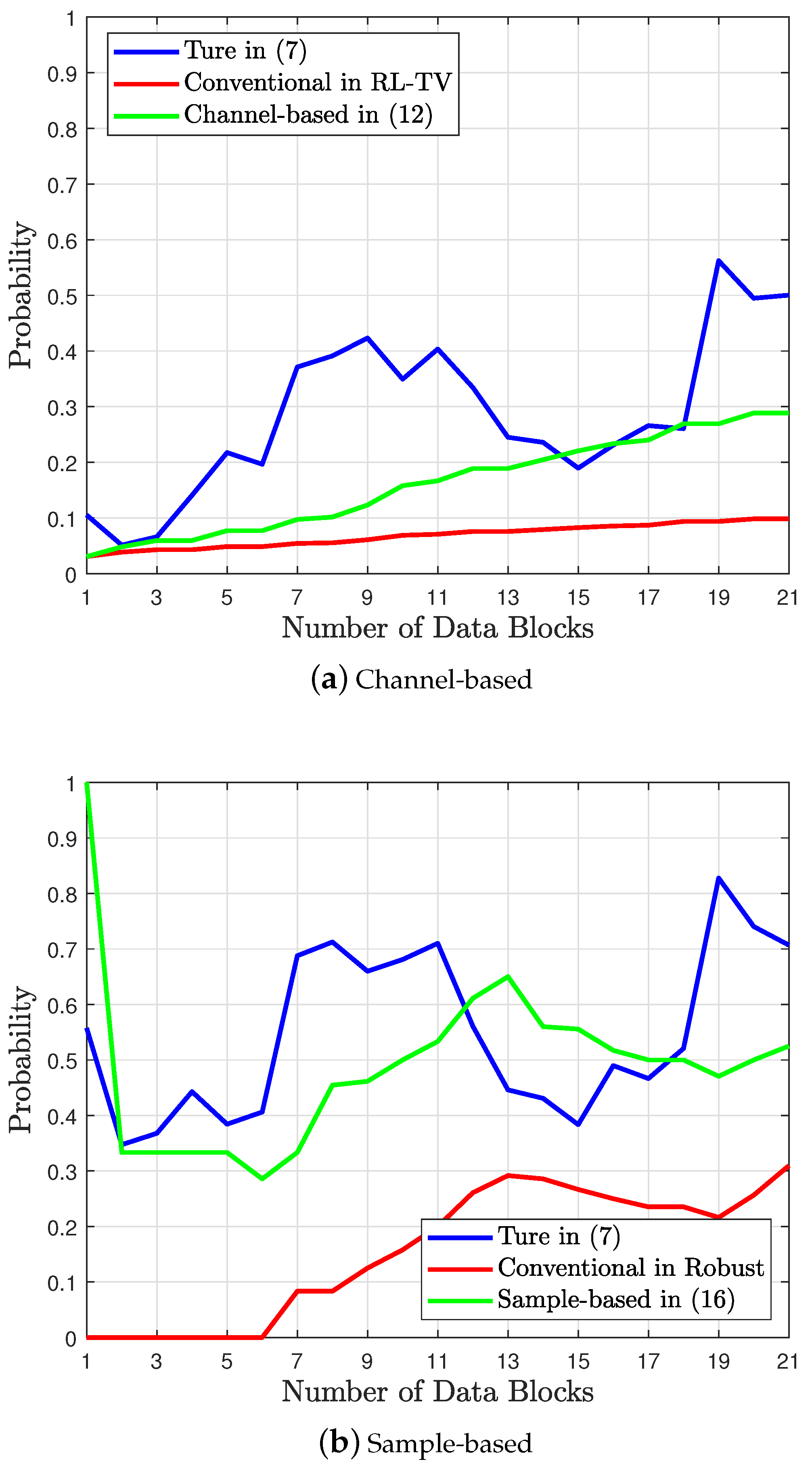
• Two probabilities influenced by time-varying channels are derived. Channel-based likelihood probability, which tracks the change in the likelihood probability based on the channel model, is simplified to reduce computational complexity compared to [38]. In addition, a sample-based likelihood probability is introduced to exploit the received data that contain the likelihood information. Unlike the conventional sample-based likelihood probability in [37] which relies on a detected symbol, the proposed approach leverages the output of the decoder. These two probabilities are then used to estimate the true probability.
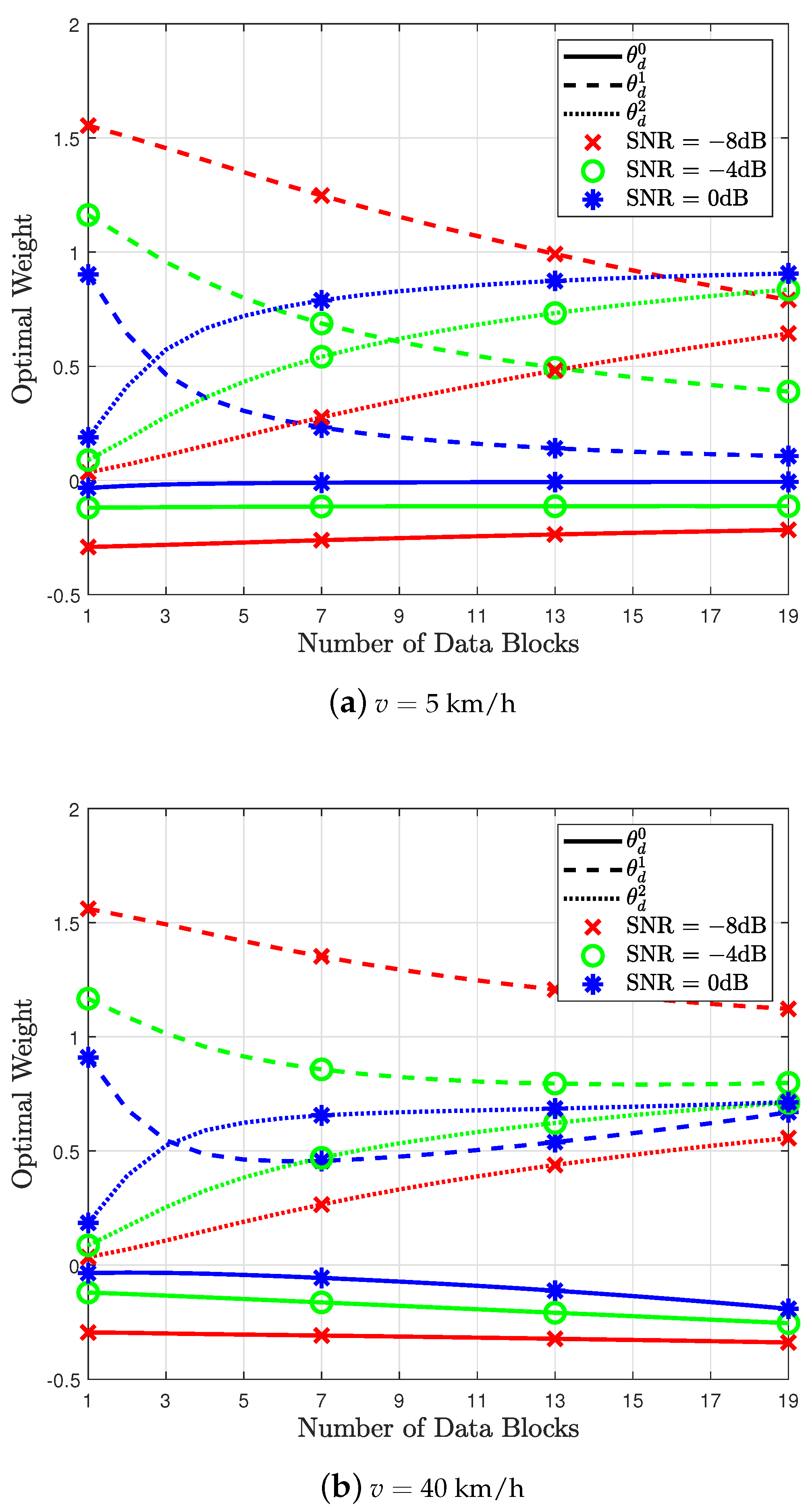
• An optimization problem is formulated to minimize the MSE between the true and estimated likelihood probabilities derived from the channel- and sample-based likelihood probabilities. Unlike previous work [19], which requires complex algorithms such as RL algorithms, the proposed method solves this problem using a regression model, eliminating the need for such intensive computation. Instead of heavy computation, the proposed method exploits the precomputed optimal weights stored in memory to calculate the regression-based likelihood probability efficiently. To further optimize the calculation, LASSO regression is introduced, allowing the model to adapt to gradual channel changes under the assumption of slow time-varying channels.
• Simulations demonstrate that the proposed method outperforms conventional methods on both slow and fast time-varying channels. This improvement results from the optimal weights, which enhance the reliability of the channel- and sample-based likelihood probabilities by fully utilizing the channel statistics and output of the decoder.

1.2. Related Works

In this subsection, the proposed method is compared with the state-of-the-art methods in terms of scalability and complexity for time-varying channels.

• The proposed method learns the likelihood probability in time-varying channels. The original approach of learning likelihood probability, initially introduced in [37], efficiently exploited input–output samples from the data detector using reinforcement learning. However, the approach in [37] was designed for time-invariant channels and faces limitations in scalability when applied to time-varying channels. To address this limitation, a channel-based likelihood probability is derived following the methodology outlined in [38]. Additionally, unlike [37], this study introduces a sample-based likelihood leveraging the decoder’s output to enhance scalability further.
• The proposed method reduces detection complexity, making it more applicable to practical systems. While a learning method that updates likelihood probability was proposed in [38] based on the on the time-varying channel model, the complexity remains a significant barrier to practical implementation. This study proposes a reduced-complexity algorithm to efficiently update the likelihood probability in time-varying channels. To achieve this, an offline learning method inspired by [39] is developed for time-varying channels. Especially, a regression-based approach is proposed to efficiently integrate channel- and sample-based likelihood probabilities.

1.3. Organization

The remainder of this study is organized as follows: Section 2 outlines the frame structure and details of the MIMO receiver with one-bit ADCs. Section 3 introduces channel and the sample-based likelihood probabilities. In addition, an optimization problem is designed to minimize the MSE between the true- and proposed likelihood probabilities. Section 4 describes the proposed solution to the optimization problem. Section 5 presents simulation results and demonstrates the effectiveness of the proposed solution. Finally, Section 6 concludes the study and discusses the main findings.

1.4. Notation

Key notations of this study are summarized in

Table 1. Key notations in this study.

Notations	Descriptions
${(·)}^H$	conjugate transpose
${(·)}^T$	transpose
$\mathbb{R}$	set of real number
$\mathbb{C}$	set of complex numbers
$\mathrm{Re}(·)$	real component of the complex number
$\mathrm{Im}(·)$	imaginary component of the complex number
$\mathrm{Sign}\left(x\right)$	function whose output is 1 for $x\ge 0$ and −1 otherwise
$\Phi (·)$	cumulative distribution of the standard normal random variable
$Q(·)$	standard Q-function
$|·|$	cardinality of the set
$\mathbb{1}\left\{\mathcal{E}\right\}$	one if the event $\mathcal{E}$ is true; otherwise, it is 0
$\mathbb{P}(·)$	probability operation
$\mathbb{E}(·)$	expectation operation
$J_0(·)$	the 0-th order Bessel function of the first kind

.

2. System Model

This section describes the model considered for the time-varying MIMO system using one-bit ADCs. The transmitter is equipped with $N_t$ antennas, and the receiver has $N_r$ antennas. The transmission frame is first explained, followed by the received signal. Finally, the considered detector is described using the likelihood.

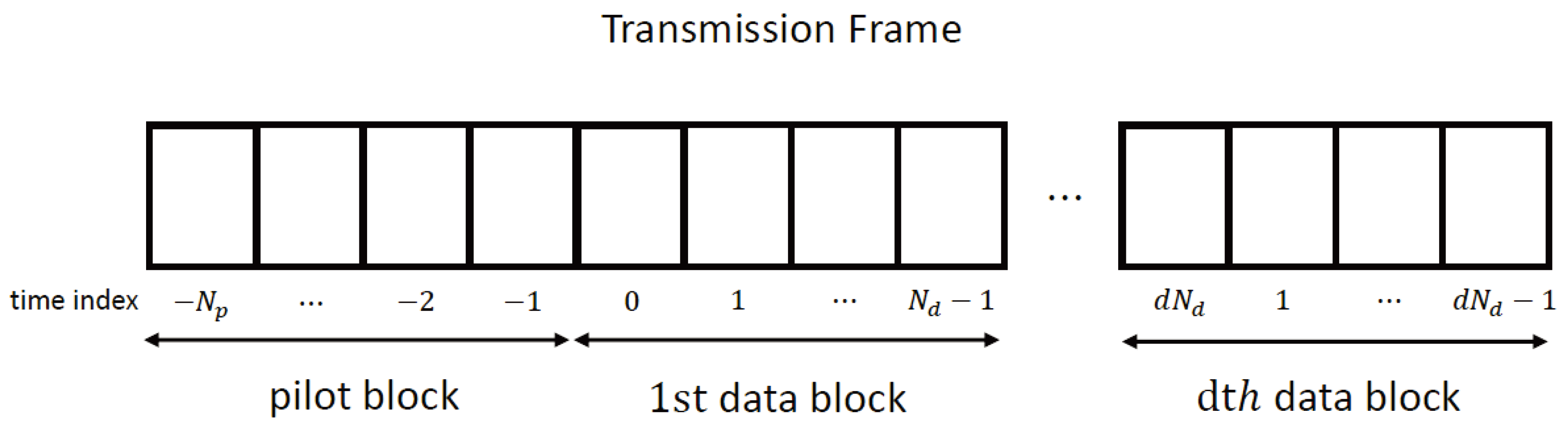
2.1. Transmitter

Each transmission frame consists of a pilot block with $N_p$ symbols and D data blocks. The d-th data block contains $N_d$ symbols, where $d\in \{1,2,\dots ,D\}$ as shown in Figure 1. The set of symbol indices in the d data block is defined as ${\mathcal{N}}_d=\{(d-1)N_d+1,\dots ,d{N}_d\}$. The information bits are encoded using a channel encoder with code rate $R_c$, and then mapped to M-ary quadrature amplitude modulation (QAM) symbols by $\overline{\mathbf{s}}\left[n\right]\in {\mathbb{C}}^{N_t\times 1}$. The QAM symbol set is $\overline{\mathcal{X}}=\{{\overline{\mathbf{s}}}_1,\dots ,{\overline{\mathbf{s}}}_K\}$ where $\mathcal{K}=\{1,2,\dots ,K\}$ is the index set of possible QAM symbol. The size $\left|\mathcal{K}\right|=M^{N_t}$ is determined by the modulation order M and the number of transmit antennas $N_t$.

2.2. Receiver

The wireless channel follows a Rayleigh fading model and is assumed to be time-variant. When the Gaussian Markov process is used to describe the time-varying nature of the channel, the channel $\overline{\mathbf{H}}\left[n\right]\in {\mathbb{C}}^{N_r\times N_t}$ at time n is given by

$$\begin{array}{c}\hfill \overline{\mathbf{H}}\left[n\right]=ϵ\overline{\mathbf{H}}[n-1]+\sqrt{1-{ϵ}^2}\overline{\Delta }\left[n\right],\end{array}$$

(1)

where $ϵ\in [0,1]$ is the temporal correlation coefficient, which is defined as $ϵ=J_0\left({\displaystyle \frac{2\pi f_{c}v{T}_s}{c}}\right)$, where $f_c$, v, $T_s$, and c denote the carrier frequency, vehicle velocity, symbol duration, and speed of light, respectively. $\overline{\Delta }\left[n\right]\in {\mathbb{C}}^{N_{\mathrm{tx}}\times N_{\mathrm{rx}}}$ is a channel evolution matrix. Given a transmitted QAM symbol $\overline{\mathbf{s}}\left[n\right]\in \overline{\mathcal{X}}$, the received signal $\overline{\mathbf{r}}\left[n\right]\in {\mathbb{C}}^{N_r\times 1}$ can be expressed as

$$\begin{array}{cc}\hfill \overline{\mathbf{r}}\left[n\right]& =\overline{\mathbf{H}}\left[n\right]\overline{\mathbf{s}}\left[n\right]+\overline{\mathbf{n}}\left[n\right],\hfill \end{array}$$

(2)

where $\overline{\mathbf{n}}\left[n\right]$ is an additive white Gaussian noise with $\mathcal{CN}(0,{\sigma }_n^2)$.

To simplify the model, the complex-valued expressions in (2) are converted into real-valued expressions as follows:

$$\begin{array}{cc}\hfill \mathbf{r}\left[n\right]& =\left[\begin{array}{c}\mathrm{Re}\left\{\overline{\mathbf{r}}\left[n\right]\right\}\\ \mathrm{Im}\left\{\overline{\mathbf{r}}\left[n\right]\right\}\end{array}\right],\mathbf{H}\left[n\right]=\left[\begin{array}{cc}\mathrm{Re}\left\{\overline{\mathbf{H}}\left[\mathbf{n}\right]\right\}& -\mathrm{Im}\left\{\overline{\mathbf{H}}\left[\mathbf{n}\right]\right\}\\ \mathrm{Im}\left\{\overline{\mathbf{H}}\left[\mathbf{n}\right]\right\}& \mathrm{Re}\left\{\overline{\mathbf{H}}\left[\mathbf{n}\right]\right\}\end{array}\right],\hfill \\ \hfill \mathbf{s}\left[n\right]& =\left[\begin{array}{c}\mathrm{Re}\left\{\overline{\mathbf{s}}\left[n\right]\right\}\\ \mathrm{Im}\left\{\overline{\mathbf{s}}\left[n\right]\right\}\end{array}\right],\mathbf{n}\left[n\right]=\left[\begin{array}{c}\mathrm{Re}\left\{\overline{\mathbf{n}}\left[n\right]\right\}\\ \mathrm{Im}\left\{\overline{\mathbf{n}}\left[n\right]\right\}\end{array}\right],\hfill \end{array}$$

(3)

where $\mathbf{r}\left[n\right]\in {\mathbb{R}}^{2N_r\times 1}$, $\mathbf{H}\left[n\right]\in {\mathbb{R}}^{2N_r\times 2N_t}$, $\mathbf{s}\left[n\right]\in {\mathbb{R}}^{2N_t\times 1}$, and $\mathbf{n}\left[n\right]\in {\mathbb{R}}^{2N_r\times 1}$.

2.3. ML Detection

After receiving signal $\mathbf{r}\left[n\right]$, a one-bit operation is applied to each real and imaginary component as

$$\begin{array}{cc}\hfill \mathbf{q}\left[n\right]& =\mathrm{sign}\left(\mathbf{r}\left[n\right]\right)=\mathrm{sign}\left(\mathbf{H}\left[n\right]\mathbf{s}\left[n\right]+\mathbf{n}\left[n\right]\right),\hfill \end{array}$$

(4)

To detect the transmitted symbol optimally, ML detection is applied as follows:

$$\begin{array}{cc}\hfill \widehat{k}\left[n\right]& =\underset{k\in \mathcal{K}}{argmax}\mathbb{P}\left(\mathbf{q}\left[n\right]\right|\mathbf{s}\left[n\right]={\mathbf{s}}_k),\hfill \end{array}$$

(5)

where ${\mathbf{s}}_k={[\mathrm{Re}{\left({\overline{\mathbf{s}}}_k\right)}^T,\mathrm{Im}{\left({\overline{\mathbf{s}}}_k\right)}^T]}^T$ is an element of the real-valued constellation set $\mathcal{X}=\{{\mathbf{s}}_1,\dots ,{\mathbf{s}}_K\}$.

The likelihood probability for ML detection with one-bit ADCs is given by

$$\begin{array}{cc}\hfill \mathbb{P}\left(\mathbf{q}\left[n\right]\right|\mathbf{s}\left[n\right]={\mathbf{s}}_k)& =\prod _{r\in \mathcal{R}}\mathbb{P}\left(q_r\left[n\right]\right|\mathbf{s}\left[n\right]={\mathbf{s}}_k)=\prod _{r:q_r\left[n\right]=+1}{p}_{r,k}\left[n\right]\prod _{r:q_r\left[n\right]=-1}1-p_{r,k}\left[n\right],\hfill \end{array}$$

(6)

where $q_r\left[n\right]$ is the r-th row of $\mathbf{q}\left[n\right]$ and the receiver antenna index is $r\in \mathcal{R}=\{1,2,\dots ,2N_r\}$. The probability $p_{r,k}$ in [19] is computed as follows:

$$\begin{array}{cc}\hfill p_{r,k}\left[n\right]& =\Phi \left(\sqrt{{\displaystyle \frac{2}{{\sigma }_n^2}}}{\mathbf{h}}_r^H\left[n\right]{\mathbf{s}}_k\right)=\Phi \left(g_{r,k}\left[n\right]\right),\hfill \end{array}$$

(7)

where ${\mathbf{h}}_r^H\left[n\right]$ is the r-th row of $\mathbf{H}\left[n\right]$ and $g_{r,k}\left[n\right]=\sqrt{{\displaystyle \frac{2}{{\sigma }_n^2}}}{\mathbf{h}}_r^H\left[n\right]{\mathbf{s}}_k$. Then, the symbol index of the ML estimate is calculated as

$$\begin{array}{cc}\hfill \widehat{k}\left[n\right]& =\underset{k\in \mathcal{K}}{argmax}\prod _{r:q_r\left[n\right]=1}{p}_{r,k}\left[n\right]\prod _{r:q_r\left[n\right]=-1}(1-p_{r,k}\left[n\right]).\hfill \end{array}$$

(8)

Using this symbol index, the ML estimate is expressed as ${\mathbf{s}}_{\widehat{k}\left[n\right]}$.

Because the true channel $\mathbf{H}\left[n\right]$ is unknown at the receiver, channel estimation is performed during the pilot transmission. After obtaining the initial estimate $\widehat{\mathbf{H}}\left[0\right]$ from the channel estimator, the initial likelihood probability $p_{r,k}\left[0\right]$ can be computed using (7). However, the accuracy of the initial probability is gradually degraded because of the time-varying nature of the channel. This is because the difference between the initially obtained channel estimate $\widehat{\mathbf{H}}\left[0\right]$ and true channel $\mathbf{H}\left[n\right]$ increases as the time index n increases.

3. Proposed Problem

This section defines the problem of improving the accuracy of the likelihood probability. To achieve this, two probabilities that can track the variation in likelihood probability are first introduced. By learning these probabilities, the optimization problem is formulated to minimize the MSE between the true and learned likelihood probabilities. Subsequently, a regression algorithm is applied to the optimization problem.

3.1. Channel-Based Likelihood Probability

This subsection introduces the channel-based likelihood probability, defined as the expected variation in the likelihood probability. Thus, the channel-based likelihood probability dynamically adjusts changes in the channel over time. Using (1), the likelihood probability is formulated as a function of the time index m, given by

$$\begin{array}{cc}\hfill p_{r,k}\left[n\right]& =\Phi \left(ϵg_{r,k}[n-1]+{\delta }_{r,k}\left[n\right]\right)=\Phi \left({ϵ}^{n-m}{g}_{r,k}\left[m\right]+{\delta }_{r,k}[n,m]\right),\hfill \end{array}$$

(9)

where ${\delta }_{r,k}\left[u\right]=\sqrt{{\displaystyle \frac{2(1-{ϵ}^2)}{{\sigma }_n^2}}}{\mathbf{\Delta }}_{r,k}^H\left[n\right]{\mathbf{s}}_k$ for $u\in \{m+1,\dots ,n\}$ and ${\delta }_{r,k}[n,m]={\sum }_{u=m+1}^n{ϵ}^{n-u}{\delta }_{r,k}\left[u\right]$. Thus, ${\delta }_{r,k}[n,m]\sim N(0,{\nu }_k[n-m])$ with ${\nu }_k\left[u\right]=(1-{ϵ}^{2u}){\displaystyle \frac{\left|\right|{\mathbf{x}}_k{\left|\right|}^2}{{\sigma }^2}}$.

Assuming the channel evolves according to a time-variant Gaussian Markov process with $ϵ\approx 1$, the difference in likelihood probabilities between times n and m is calculated as follows:

$$\begin{array}{cc}\hfill p_{r,k}\left[n\right]-p_{r,k}\left[m\right]& =\Phi \left({ϵ}^{n-m}{g}_{r,k}\left[m\right]+{\delta }_{r,k}[n,m]\right)-\Phi \left(g_{r,k}\left[m\right]\right)\hfill \\ \hfill & \stackrel{\left(a\right)}{\approx }-((1-{ϵ}^{n-m})g_{r,k}\left[m\right]-{\delta }_{r,k}[n,m])\varphi \left({\displaystyle \frac{(1-{ϵ}^{n-m})g_{r,k}\left[m\right]+{\delta }_{r,k}[n,m]}{2}}\right)\hfill \\ \hfill & =-2((1-{ϵ}^{n-m})g_{r,k}\left[m\right]-{\delta }_{r,k}[n,m]){\displaystyle \frac{1}{\sqrt{2\pi \times 4}}}{e}^{{\displaystyle \frac{-{\left({\delta }_{r,k}[n,m]+(1+{ϵ}^{n-m})g_{r,k}\left[m\right]\right)}^2}{2\times 4}}},\hfill \end{array}$$

(10)

where the approximation in $\left(a\right)$ is valid as $\Phi \left(x\right)-\Phi \left(a\right)\approx (x-a){\Phi }^{\prime }\left({\displaystyle \frac{x+a}{2}}\right)$ when $x\to a$ under the assumption $ϵ\approx 1$. Here, ${\Phi }^{\prime }\left(x\right)=\varphi \left(x\right)={\displaystyle \frac{1}{\sqrt{2\pi }}}exp(-{\displaystyle \frac{x^2}{2}})$.

With an assumed expected value of $\mathbb{E}\left[p_{r,k}\left[m\right]\right]={\widehat{p}}_{r,k}\left[m\right]$, the expectation of (10) can be further simplified to

$$\begin{array}{cc}\hfill \mathbb{E}\left[p_{r,k}\left[n\right]\right]& \approx {\widehat{p}}_{r,k}^{\mathrm{channel}}\left[m\right]-2\left((1-{ϵ}^{n-m}){\widehat{g}}_{r,k}\left[m\right]\right)\mathbb{E}\left[{\displaystyle \frac{1}{\sqrt{2\pi \times 4}}}{e}^{{\displaystyle \frac{-{\left({\delta }_{r,k}[n,m]+(1+{ϵ}^{n-m}){\widehat{g}}_{r,k}\left[m\right]\right)}^2}{2\times 4}}}\right]\hfill \\ \hfill & \stackrel{\left(a\right)}{\approx }{\widehat{p}}_{r,k}^{\mathrm{channel}}\left[m\right]-{\displaystyle \frac{2(1-{ϵ}^{n-m}){\widehat{g}}_{r,k}\left[m\right]}{\sqrt{2\pi ({\nu }_k[n-m]+4)}}}{e}^{-{\displaystyle \frac{{\left((1+{ϵ}^{n-m}){\widehat{g}}_{i,k}\left[m\right]\right)}^2}{2({\nu }_k[n-m]+4)}}},\hfill \end{array}$$

(11)

where $\mathbb{E}\left\{{\displaystyle \frac{1}{\sqrt{2\pi {\sigma }^2}}}{e}^{-{\displaystyle \frac{{(X-\mu )}^2}{2{\sigma }^2}}}\right\}={\displaystyle \frac{1}{\sqrt{2\pi ({\nu }^2+{\sigma }^2)}}}{e}^{-{\displaystyle \frac{{\mu }^2}{2({\nu }^2+{\sigma }^2)}}}$ is applied in $\left(a\right)$ when $X\sim \mathcal{N}(0,{\nu }^2)$.

The derivation in (11), which removes the term ${\delta }_{r,k}[n,m]$, differs from that in [38], resulting in reduced computational complexity.

Consequently, the channel-based likelihood probability under the assumption that $\mathbb{E}\left[p_{r,k}\left[m\right]\right]={\widehat{p}}_{r,k}^{\mathrm{channel}}\left[m\right]$, and tracking from time m, is given by

$$\begin{array}{cc}\hfill p_{r,k}^{\mathrm{channel}}\left[n\right]& ={\widehat{p}}_{r,k}^{\mathrm{channel}}\left[m\right]-f({\Phi }^{-1}\left({\widehat{p}}_{r,k}^{\mathrm{channel}}\left[m\right]\right),{\nu }_k^{n-m},{ϵ}^{n-m}),\hfill \end{array}$$

(12)

where $f(g,\nu ,ϵ)={\displaystyle \frac{2(1-ϵ)g}{\sqrt{2\pi (\nu +4)}}}{e}^{-{\displaystyle \frac{{\left((1+ϵ)g\right)}^2}{2(\nu +4)}}}$.

3.2. Sample-Based Likelihood Probability

This subsection details the derivation of the sample-based likelihood probability constructed based on the received signals. The probability $p_{r,k}$ in (7) can be defined using the conditional probability formula:

$$\begin{array}{cc}\hfill p_{r,k}& =\mathbb{P}(q_r\left[n\right]=1|\mathbf{s}\left[n\right]={\mathbf{s}}_k)={\displaystyle \frac{\mathbb{P}(q_r\left[n\right]=1,\mathbf{s}\left[n\right]={\mathbf{s}}_k)}{\mathbb{P}(\mathbf{s}\left[n\right]={\mathbf{s}}_k)}},\hfill \end{array}$$

(13)

where each probability term in (13) is defined as follows:

$$\begin{array}{cc}\hfill \mathbb{P}(q_r\left[n\right]=1,\mathbf{s}\left[n\right]={\mathbf{s}}_k)& =\underset{{\displaystyle \sum _{m\le n}}\mathbb{1}\{k\left[m\right]=k\}\to \infty }{lim}{\displaystyle \frac{{\displaystyle \sum _{m\le n}}{\tilde{q}}_r\left[m\right]\mathbb{1}\{k\left[m\right]=k\}}{n}},\hfill \\ \hfill \mathbb{P}(\mathbf{s}\left[n\right]={\mathbf{s}}_k)& =\underset{{\displaystyle \sum _{m\le n}}\mathbb{1}\{k\left[m\right]=k\}\to \infty }{lim}{\displaystyle \frac{{\displaystyle \sum _{m\le n}}\mathbb{1}\{k\left[m\right]=k\}}{n}}.\hfill \end{array}$$

(14)

where ${\tilde{q}}_r\left[n\right]$ is a function that assumes the value of 1 if $q_r\left[n\right]=1$ and 0 otherwise.

As the transmitted symbol index $k\left[m\right]$ is not available at the receiver, the probabilities in (14) cannot be computed directly; instead, they are approximated using the detected symbol index $\widehat{k}\left[m\right]$, given by

$$\begin{array}{cc}\hfill \mathbb{P}(q_r\left[n\right]=1,\mathbf{s}\left[n\right]={\mathbf{s}}_k)& \approx {\displaystyle \frac{{\displaystyle \sum _{m\le n}}{\tilde{q}}_r\left[m\right]\mathbb{1}\{\widehat{k}\left[m\right]=k\}}{n}},\hfill \\ \hfill \mathbb{P}(\mathbf{s}\left[n\right]={\mathbf{s}}_k)& \approx {\displaystyle \frac{{\displaystyle \sum _{m\le n}}\mathbb{1}\{\widehat{k}\left[m\right]=k\}}{n}}.\hfill \end{array}$$

(15)

These approximations converge to the true probabilities when n becomes sufficiently large [19].

However, the detected symbol index $\widehat{k}\left[n\right]$ is often inaccurate compared to the true symbol index with a high probability. To address this, symbol refinement is proposed, in which the decoder’s capability is exploited to estimate the true symbol index $k\left[n\right]$. Thus, unlike in [19], the re-detected symbol index ${\widehat{k}}_{\mathrm{dec}}\left[n\right]$ is used to obtain the sample-based probability as follows:

$$\begin{array}{cc}\hfill p_{r,k}^{\mathrm{sample}}\left[n\right]& \approx {\displaystyle \frac{{\displaystyle \sum _{m\le n}}{\tilde{q}}_r\left[m\right]\mathbb{1}\{{\widehat{k}}_{\mathrm{dec}}\left[m\right]=k\}}{{\displaystyle \sum _{m\le n}}\mathbb{1}\{{\widehat{k}}_{\mathrm{dec}}\left[m\right]=k\}}}.\hfill \end{array}$$

(16)

Notably, the proposed likelihood probability in (17) occurs after each data block and the decoder output is available to calculate the sample-based likelihood probability.

3.3. Optimization Problem

The proposed likelihood probability, ${\widehat{p}}_{r,k}\left[n\right]$, is formulated as a linear regression of the channel-based likelihood probability in (12) and the sample-based likelihood probability in (16). This approach is used because the channel-based likelihood probability captures the change in channel statistics, whereas the sample-based likelihood probability trains the true likelihood probability from the quantized received signal and re-detected symbol index. The model for the proposed likelihood is expressed as follows:

$$\begin{array}{cc}\hfill {\widehat{p}}_{r,k}\left[n\right]\left({\mathbf{\Theta }}_n\right)& ={\theta }_n^0+{\theta }_n^1{p}_{r,k}^{\mathrm{channel}}\left[n\right]+{\theta }_n^2{p}_{r,k}^{\mathrm{sample}}\left[n\right],\hfill \end{array}$$

(17)

where ${\mathbf{\Theta }}_n={[{\theta }_n^0,{\theta }_n^1,{\theta }_n^2]}^T$ is the model parameter. Using this model, the optimization problem is defined as follows:

$$\begin{array}{cc}\hfill {\mathbf{\Theta }}_n^{\star }& =\underset{{\mathbf{\Theta }}_n}{argmin}\sum _{r\in \mathcal{R}}\sum _{k\in \mathcal{K}}{\parallel p_{r,k}\left[n\right]-{\widehat{p}}_{r,k}\left[n\right]\left({\mathbf{\Theta }}_n\right)\parallel }^2,\hfill \end{array}$$

(18)

where ${\mathbf{\Theta }}_n^{\star }={[{\left({\theta }_n^0\right)}^{\star },{\left({\theta }_n^1\right)}^{\star },{\left({\theta }_n^2\right)}^{\star }]}^T$.

Directly solving the optimization problem in (18) is difficult due to the nonlinear nature of the function $\Phi (·)$, and the fact that sample-based likelihood probability cannot be readily represented in a mathematically convenient form. To address these issues, linear regression is used as an alternative approach to determine the model parameter ${\mathbf{\Theta }}_n$.

4. Proposed Solution

This section formulates the proposed likelihood probability to solve the optimization problem in (18). To address this problem, a linear regression approach is applied to (18). Because the channel is slowly varying in realistic scenarios, a regularization technique is introduced to further optimize the algorithm. Consequently, the structure of the proposed receiver is outlined, along with the algorithmic procedure.

4.1. Linear Regression

This subsection introduces a linear regression approach to obtain the model parameter ${\mathbf{\Theta }}_n$. However, solving the regression for individual time index n increases the complexity of both learning and applying ${\mathbf{\Theta }}_n$. To address this issue, learning and applications are considered on a per-data-block basis. Subsequently, the optimization problem in (18) is re-formulated as follows:

$$\begin{array}{cc}\hfill {\mathbf{\Theta }}_d^{\star }& =\underset{{\mathbf{\Theta }}_d}{argmin}\sum _{n\in {\mathcal{N}}_d}\sum _{r\in \mathcal{R}}\sum _{k\in \mathcal{K}}{\parallel p_{r,k}\left[n\right]-{\widehat{p}}_{r,k}\left[n\right]\left({\mathbf{\Theta }}_d\right)\parallel }^2,\hfill \end{array}$$

(19)

where ${\mathbf{\Theta }}_d=={[{\theta }_d^0,{\theta }_d^1,{\theta }_d^2]}^T$. Linear regression is a well-known technique for solving the optimization problem in (19). To achieve this outcome, the matrices ${\mathbf{X}}_d\in {\mathbb{R}}^{N_d\times 3}$ and ${\mathbf{y}}_d\in {\mathbb{R}}^{N_d\times 1}$ are, respectively, defined as

$$\begin{array}{ll}\hfill {\mathbf{\Phi }}_d& =\left[\begin{array}{lll}1& p_{r,k}^{\mathrm{channel}}[(d-1)N_d+1]& p_{r,k}^{\mathrm{sample}}[(d-1)N_d+1]\\ 1& p_{r,k}^{\mathrm{channel}}[(d-1)N_d+2]& p_{r,k}^{\mathrm{sample}}[(d-1)N_d+2]\\ ⋮& \hspace{1em}\hspace{1em}\hspace{1em}\hspace{1em}⋮& \hspace{1em}\hspace{1em}\hspace{1em}\hspace{1em}⋮\\ 1& p_{r,k}^{\mathrm{channel}}\left[d{N}_d\right]& p_{r,k}^{\mathrm{sample}}\left[d{N}_d\right]\end{array}\right],{\mathbf{y}}_d=\left[\begin{array}{l}{p}_{r,k}[(d-1)N_d+1]\\ p_{r,k}[(d-1)N_d+2]\\ \hspace{1em}\hspace{1em}\hspace{1em}\hspace{1em}⋮\\ p_{r,k}\left[d{N}_d\right]\end{array}\right].\hfill \end{array}$$

(20)

Then, the optimal parameter ${\mathbf{\Theta }}_d^{\star }$ of (19) can be derived as follows:

$$\begin{array}{cc}\hfill {\mathbf{\Theta }}_d^{\star }& ={\left({\mathbf{\Phi }}_d^T{\mathbf{\Phi }}_d\right)}^{-1}{\mathbf{\Phi }}_d^T{\mathbf{y}}_d.\hfill \end{array}$$

(21)

The optimal parameters in (21) are suboptimal because they are obtained from a limited number of samples. Using the optimal parameters, the proposed probability at the end of the d-th data block is expressed as follows:

$$\begin{array}{cc}\hfill {\widehat{p}}_{r,k}^{\mathrm{pro}}\left({\mathbf{\Theta }}_d^{\star }\right)& ={\left({\theta }_d^0\right)}^{\star }+{\left({\theta }_d^1\right)}^{\star }{p}_{r,k}^{\mathrm{channel}}\left[d{N}_d\right]+{\left({\theta }_d^2\right)}^{\star }{p}_{r,k}^{\mathrm{sample}}\left[d{N}_d\right].\hfill \end{array}$$

(22)

4.2. Regularization

In this subsection, the effective regression technique is discussed under the slow-fading channel. The linear regression in (19) provides a reasonable solution for approximating the true probability. However, under the assumption of a slow-fading channel, the probability changes slowly. Regularization techniques such as ridge and LASSO regressions are effective in preventing abrupt changes. In this study, LASSO regression is employed because it not only prevents sudden changes but also eliminates irrelevant parameters. This elimination improves memory utilization by reducing the number of weights and by simplifying the computation in (22). To achieve this, LASSO regression is formulated as follows:

$$\begin{array}{cc}\hfill {\mathbf{\Theta }}_d^{\star }& =\underset{{\mathbf{\Theta }}_d}{argmin}\sum _{n\in {\mathcal{N}}_d}\sum _{r\in \mathcal{R}}\sum _{k\in \mathcal{K}}\parallel p_{r,k}\left[n\right]-{\widehat{p}}_{r,k}\left[n\right]\left({\mathbf{\Theta }}_d\right){\parallel }^2+\lambda \parallel {\mathbf{\Theta }}_d\parallel ,\hfill \end{array}$$

(23)

where $\lambda$ is a tuning value that controls the trade-off between fit and sparsity in the regression coefficient estimates. In particular, LASSO regression exploits the $L_1$ norm, which encourages certain parameters to be exactly zero, promoting sparsity in the solution. This allows significant parameters to be identified and extracted using a regularization technique. Although solving the LASSO regression is more complicated than solving the linear regression, the proposed method utilizes the pre-computed optimal parameters. By eliminating insignificant parameters, this approach helps efficiently calculate the proposed likelihood probability in (22) during transmission.

4.3. Proposed Receiver

This subsection describes the proposed receiver structure. The receiver initiates by estimating the channel during pilot transmission. The initial probability ${\widehat{p}}_{r,k}\left[0\right]$ can then be obtained using the channel estimate. During data transmission, the receiver calculates the probability proposed in (12). The calculated likelihood probability is used in the log-likelihood ratio (LLR) calculation, given by

$$\begin{array}{cc}\hfill LLR\left(b_{i,j}\left[n\right]\right)& =log{\displaystyle \frac{\mathbb{P}\left(\mathbf{q}\left[n\right]\right|b_{i,j}\left[n\right]=1)}{\mathbb{P}\left(\mathbf{q}\left[n\right]\right|b_{i,j}\left[n\right]=0)}}=log{\displaystyle \frac{{\displaystyle \sum _{{\mathbf{s}}_k\in {\mathcal{X}}_{i,j}^1}}\mathbb{P}\left(\mathbf{q}\left[n\right]\right|\mathbf{s}\left[n\right]={\mathbf{s}}_k)}{\sum _{{\mathbf{s}}_k\in {\mathcal{X}}_{i,j}^0}\mathbb{P}\left(\mathbf{q}\left[n\right]\right|\mathbf{s}\left[n\right]={\mathbf{s}}_k)}}\hfill \\ \hfill & \stackrel{\left(a\right)}{=}log{\displaystyle \frac{{\displaystyle \sum _{{\mathbf{s}}_k\in {\mathcal{X}}_{i,j}^1}}\widehat{\mathbb{P}}\left(\mathbf{q}\left[n\right]\right|\mathbf{s}\left[n\right]={\mathbf{s}}_k)}{\sum _{{\mathbf{s}}_k\in {\mathcal{X}}_{i,j}^0}\widehat{\mathbb{P}}\left(\mathbf{q}\left[n\right]\right|\mathbf{s}\left[n\right]={\mathbf{s}}_k)}}=log{\displaystyle \frac{{\displaystyle \sum _{{\mathbf{s}}_k\in {\mathcal{X}}_{i,j}^1}}\left({\displaystyle \prod _{r:q_r\left[n\right]=1}}{\widehat{p}}_{r,k}^{\mathrm{pro}}{\displaystyle \prod _{r:q_r\left[n\right]=-1}}(1-{\widehat{p}}_{r,k}^{\mathrm{pro}})\right)}{{\displaystyle \sum _{{\mathbf{s}}_k\in {\mathcal{X}}_{i,j}^0}}\left({\displaystyle \prod _{r:q_r\left[n\right]=1}}{\widehat{p}}_{r,k}^{\mathrm{pro}}{\displaystyle \prod _{r:q_r\left[n\right]=-1}}(1-{\widehat{p}}_{r,k}^{\mathrm{pro}})\right)}},\hfill \end{array}$$

(24)

where the proposed likelihood probability in (17) is applied to the true likelihood probability $\left(a\right)$. $b_{i,j}\left[n\right]\in \{0,1\}$ is the j-th bit of the i-th stream and ${\mathcal{X}}_{i,j}^b$ is the set of symbols ${\mathbf{s}}_k$ for which $b_{i,j}=b\in \{0,1\}$. This LLR value is used to obtain the decoded data ${\widehat{b}}_{i,j}$ from the channel decoder.

At the end of the data block, the receiver computes the channel-based likelihood probability $p_{r,k}^{\mathrm{channel}}$ using (12) and the sample-based likelihood probability using (16) based on the channel decoder output. Following these calculations, the proposed receiver updates the combined likelihood probabilities ${\widehat{p}}_{r,k}^{\mathrm{pro}}$ by integrating both the channel- and sample-based likelihood values. The optimal weights ${\mathbf{\Theta }}_d^{\star }$, stored in memory, are selected according to the data block index d to effectively combine two likelihood probabilities. The complete step-by-step procedure of the proposed receiver is presented in Algorithm 1.

Algorithm 1: Procedure of the Proposed Receiver

1 Pilot Block

2 Obtain initial channel estimate $\widehat{\mathbf{H}}\left[0\right]=\left[{\widehat{\mathbf{h}}}_1\left[0\right],\cdots ,{\widehat{\mathbf{h}}}_{N_r}\left[0\right]\right]$.

3 Calculate the initial channel-based likelihood probability $p_{r,k}^{\mathrm{channel}}\left[0\right]$, $r\in \mathcal{R},k\in \mathcal{K}$ from $\widehat{\mathbf{H}}\left[0\right]$.

4 Set the proposed likelihood probability ${\widehat{p}}_{r,k}^{\mathrm{pro}}\leftarrow p_{r,k}^{\mathrm{channel}}\left[0\right]$, $r\in \mathcal{R},k\in \mathcal{K}$.

5 Data Block

6 for $d=1$ to D do$\phantom{(}$

7   for $n=1$ to $N_d$ do$\phantom{(}$

8     Compute LLR in (24) based on the proposed likelihood probability ${\widehat{p}}_{r,k}^{\mathrm{pro}}$.

9     Obtain decoded data ${\widehat{b}}_{i,j}$ from the channel decoder.

10   end$\phantom{(}$

11   Bring the optimal weight ${\mathbf{\Theta }}_d^{\star }$ in memory trained using (21).

12   Update channel-based likelihood probability $p_{r,k}^{\mathrm{channel}}$ from (12) and $\mathbb{E}\left[p_{r,k}\left[d{N}_d\right]\right]={\widehat{p}}_{r,k}^{\mathrm{channel}}\left[d{N}_d\right]$.

13   The sample-based likelihood probabilities $p_{r,k}^{\mathrm{sample}}$ are updated from the decoding output in (16).

14   Calculate the proposed likelihood probability ${\widehat{p}}_{r,k}^{\mathrm{pro}}\leftarrow {\left({\theta }_d^0\right)}^{\star }+{\left({\theta }_d^1\right)}^{\star }{p}_{r,k}^{\mathrm{channel}}\left[d{N}_d\right]+{\left({\theta }_d^2\right)}^{\star }{p}_{r,k}^{\mathrm{sample}}\left[d{N}_d\right]$ using (22).

15 end

5. Simulation Results

Simulations are performed using Matrix Laboratory (MATLAB). The optimal weights in (19) and (23) are obtained through the statistics and machine learning toolbox. The obtained optimal weights are then used in simulations to evaluate the frame error rate (FER) and MSE over 10,000 iterations. The antenna configuration used is $(N_t,N_r)=(4,8)$. For the time-variant channel, a carrier frequency $f_c=3.5$ GHz, and a sampling period of $T_s=16.67$$\mu$s is considered, as specified in [40]. Velocities of $v=5$ km/h and $v=40$ km/h, represent slow and fast time-varying channels, respectively. The information bits are encoded using a turbo encoder at a rate $R_c={\displaystyle \frac{1}{2}}$. A modulation order of 4-$QAM$ is applied to the encoded bits, resulting in a constellation size of $K=M^{N_t}=256$. The frame structure consists of one pilot with $N_p=32$ and $D=20$ data blocks with $N_d=128$. A linear MMSE method was applied to obtain the initial channel estimation during pilot transmission. The signal-to-noise ratio (SNR), denoted as $E_b/N_0$, is defined as ${\displaystyle \frac{1}{{log}_2\left|\mathcal{X}\right|{\sigma }_n^2}}$.

For performance benchmarking, the following methods are considered:

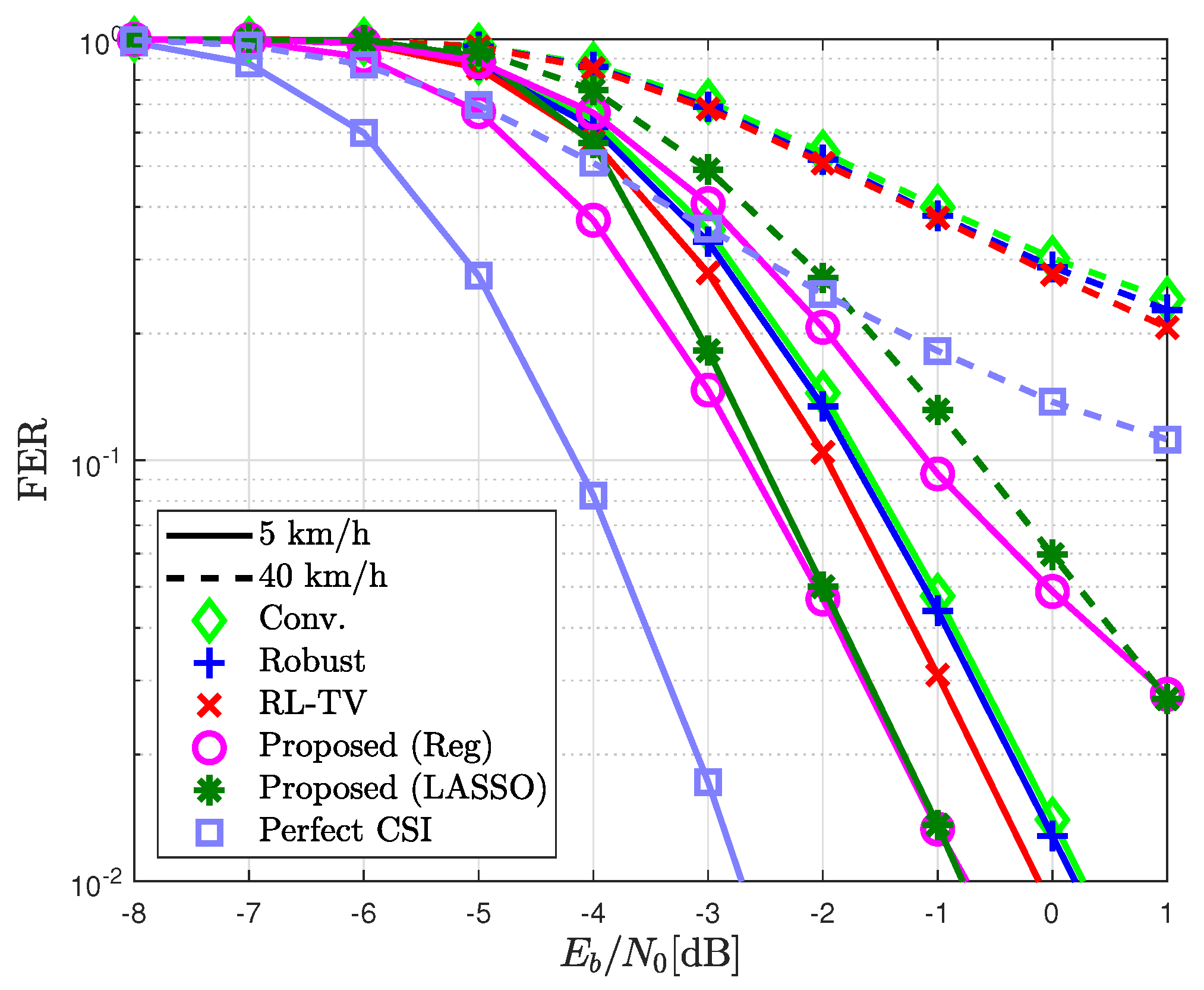
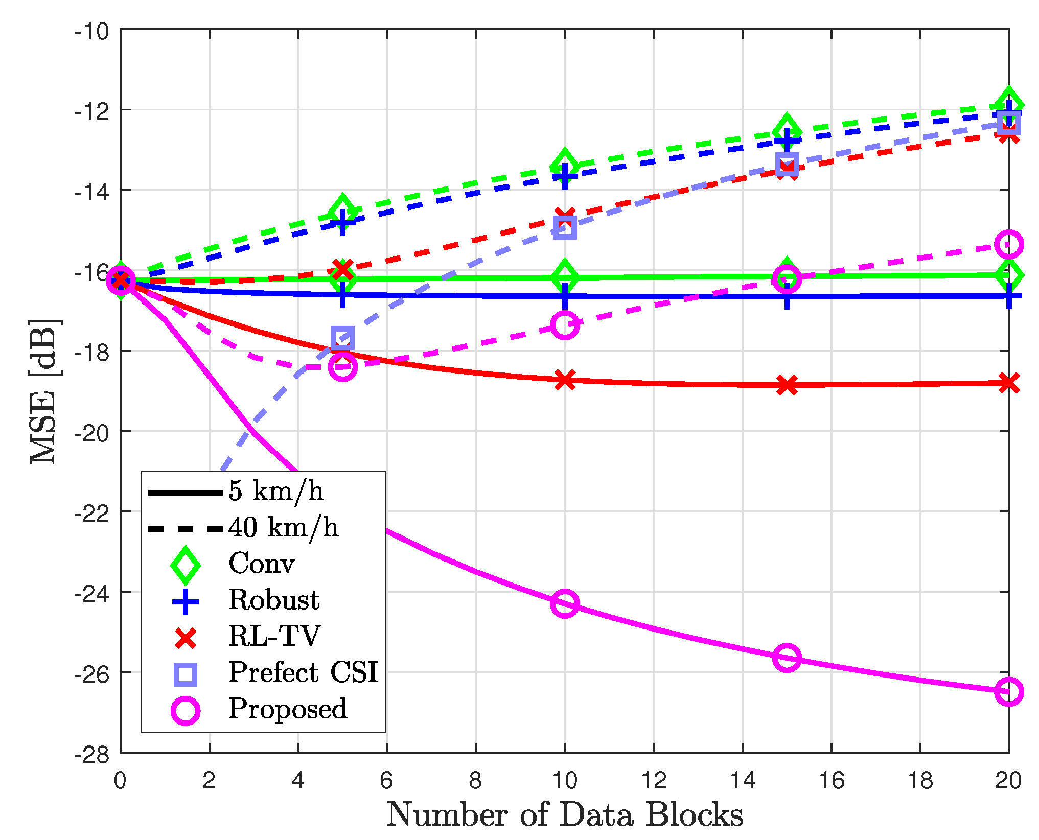
• Perfect CSI: This represents the optimal case in time-invariant channels, where the likelihood probability is obtained using perfect channel state information (CSI) of $\mathbf{H}\left[0\right]$. Note that the resulting likelihood probability remains constant over time, and thus is not optimal in time-varying channels.
• Conv.: This conventional method calculates the probability $p_{r,k}^{\mathrm{channel}}\left[0\right]$ based on channel estimates $\widehat{\mathbf{H}}\left[0\right]$ obtained during pilot transmission. In this method, the likelihood probability remains fixed during data transmission.
• Robust: Developed in [37] for time-invariant MIMO channels. This method calculates the likelihood probability using an RL algorithm, where the initial likelihood probability is optimally combined with the empirical-based likelihood probability obtained from the detected symbol.
• RL-TV: Introduced in [38] for time-varying MIMO channels, this method calculates the likelihood probability using an RL algorithm, where the model-based likelihood probability and the quantized received signal are optimally combined. Notably, the sample refinement scheme is not used in this study where all input–output samples are used to update the likelihood probability when the cyclic redundancy check (CRC) is correct. This exclusion is intended to ensure a fair comparison with other methods.
• Proposed: The proposed method exploits the likelihood probability from (22), where both the channel- and the sample-based likelihood probabilities are learned via linear regression. The proposed (Reg) denotes the case when the optimization problem in (19) is applied, while the proposed (LASSO) refers to when the regularization technique in (23) is applied. The precise definitions for the channel- and sample-based likelihood probabilities differ from those in [37] and [38], respectively.

In Figure 2, the channel- and sample-based likelihood probabilities are compared with true likelihood probability in (7) under fast-fading channels. In Figure 2a, the conventional model-based likelihood probability from [38] is compared with the channel-based likelihood probability in (12). While the conventional model-based likelihood probability shows a gradual response to changes in the true likelihood probabilities in (7), the channel-based likelihood probability more efficiently captures these changes. Note that the channel-based likelihood probability is derived in (10) under the assumption of slow-fading channels $ϵ\approx 1$. As a result, it exhibits slower changes compared to the true likelihood probability in fast-fading channels. In Figure 2b, the sample-based likelihood probability in (16) outperforms the conventional empirical-based likelihood probability from [37] in capturing rapid changes in the true likelihood probability. This improvement is attributed to the decoder’s output, which provides more accurate information about the channel.

In Figure 3, the optimal weights of the linear regression for the proposed method are shown as a function of d. As the number of data blocks increases, the accuracy of the sample-based likelihood improves. Thus, the weight ${\theta }_d^2$ for the sample-based likelihood probability increases, while the weight ${\theta }_d^1$ for the channel-based likelihood probability decreases. In contrast, the constant weight ${\theta }_d^0$ approaches zero with the increase in d in the slow-fading channels. In addition, when the SNR increases, the convergence speed increases because the correctly decoded output improves the accuracy of the sample-based likelihood probability. Compared to slow-fading channels, the increase in the sample-based likelihood probability is smaller in the fast-fading channels, where the channel-based likelihood probability dominantly affects the overall likelihood probability.

The optimal weights for the LASSO regression are simulated with $\lambda ={10}^{-2}$ for slow fading channels and $\lambda ={10}^{-1}$ for fast fading channels, as shown in Figure 4. Both figures show a similar overall trend to the linear regression in Figure 3. However, in the LASSO regression, the optimal weight ${\theta }_d^0$ is exactly zero, indicating that the constant weight is less significant than the weights for the channel- and sample-based likelihood probabilities. Compared to slow-fading channels, the weights for the channel-based likelihood probability in fast-fading channels are larger, as the channel-based likelihood probability can more effectively track changes in the likelihood probability for the subsequent block.

The FERs for the different detection methods are plotted in Figure 5 to demonstrate the effectiveness of the proposed method in both the slow and fast fading channels. For the LASSO method, the optimal weights from Figure 4 are applied in both channel conditions. The Conv. and Robust methods exhibit poor performance owing to their inability to track the true likelihood probability. The FER of the RL-TV exhibits a slight improvement, indicating that it struggles to follow the channel variations. This result contrasts with [38], where the sample-refinement scheme primarily addresses temporal channel variation compensation. The proposed (Reg) and proposed (LASSO) methods achieve SNR gains of approximately 0.8 dB and 0.7 dB over the RL-TV in slow fading channels at an FER of ${10}^{-1}$, while the SNR gain in fast fading channels is substantial compared to conventional methods. This improvement is attributed to the proposed methods’ ability to track changes in the likelihood probability by optimally combining both channel- and sample-based likelihood probabilities. Note that the proposed (LASSO) method uses only two weights to calculate the proposed likelihood probability, while the proposed (Reg) method uses three weights.

Figure 6 presents the MSE between the true and proposed likelihood probabilities, i.e., $\mathbb{E}\{\parallel p_{r,k}-{\widehat{p}}_{r,k}{\parallel }^2\}$. The proposed method achieves a lower MSE compared to the conventional methods in both slow and fast fading channels. The MSEs of the perfect CSI and Conv. methods are gradually degraded in time-varying channels because they do not update the likelihood probability and fail to adapt to channel variations. In contrast, the MSEs of RL-TV and proposed methods improve as d increases in slow-fading channels, as both methods derive the likelihood probabilities based on time-varying channel models. The proposed method outperforms the RL-TV method due to its ability to learn the optimal weights that minimize the MSE between the true and learned likelihood probabilities, which effectively tracks temporal variations in the channel.

6. Conclusions

A regression-based approach for tracking changes in the likelihood in time-varying MIMO systems using one-bit ADCs was introduced. The proposed method utilized channel statistics to derive a channel-based likelihood probability and the decoded output to derive a sample-based likelihood probability. The optimization problem for the weighted linear combination of the two probabilities was formulated by minimizing the expected MSE. A linear regression method was applied to solve the problem, with a regularization technique incorporated to optimize the calculation. In particular, simulation results demonstrated that the proposed method outperformed conventional methods by effectively capturing the changes in the likelihood.

The future direction of this study is to explore other regression techniques such as polynomial and Bayesian regressions. These advanced regression methods can improve the fit to the true likelihood probability. In addition to exploring different regression techniques, better features should be extracted from the channel model and received symbols. Features that provide more relevant information about the channel can further improve the regression performance. Further improvement will address the power consumption and computational complexity challenges associated with mmWave and THz communications in time-varying MIMO systems using one-bit ADCs.

References

- Swindlehurst, A.L.; Ayanoglu, E.; Heydari, P.; Capolino, F. Millimeter-Wave Massive MIMO: The Next Wireless Revolution? IEEE Commun. Mag. 2014, 52, 56–62. [Google Scholar] [CrossRef]
- Rangan, S.; Rappaport, T.S.; Erkip, E. Millimeter-Wave Cellular Wireless Networks: Potentials and Challenges. Proc. IEEE 2014, 102, 366–385. [Google Scholar] [CrossRef]
- Busari, S.A.; Huq, K.M.S.; Mumtaz, S.; Dai, L.; Rodriguez, J. Millimeter-Wave Massive MIMO Communication for Future Wireless Systems: A survey. IEEE Commun. Surv. Tutor. 2017, 20, 836–869. [Google Scholar] [CrossRef]
- Wang, X.; Kong, L.; Kong, F.; Qiu, F.; Xia, M.; Arnon, S.; Chen, G.; Rodriguez, J. Millimeter Wave Communication: A Comprehensive Survey. IEEE Commun. Surv. Tutor. 2018, 20, 1616–1653. [Google Scholar] [CrossRef]
- Uwaechia, A.N.; Mahyuddin, N.M. A Comprehensive Survey on Millimeter Wave Communications for Fifth-Generation Wireless Networks: Feasibility and Challenges. IEEE Access 2020, 8, 62367–62414. [Google Scholar] [CrossRef]
- Bang, J.; Chung, H.; Hong, J.; Seo, H.; Choi, J.; Kim, S. Millimeter-Wave Communications: Recent Developments and Challenges of Hardware and Beam Management Algorithms. IEEE Commun. Mag. 2021, 59, 86–92. [Google Scholar] [CrossRef]
- Walden, R.H. Analog-to-Digital Converter Survey and Analysis. IEEE J. Sel. Areas Commun. 1999, 17, 539–550. [Google Scholar] [CrossRef]
- Murmann, B. ADC Performance Survey 1997–2024. [Online]. Available online: https://github.com/bmurmann/ADC-survey (accessed on 13 November 2024).
- Fan, L.; Jin, S.; Wen, C.K.; Zhang, H. Uplink Achievable Rate for Massive MIMO Systems With Low-Resolution ADC. IEEE Commun. Lett. 2015, 19, 2186–2189. [Google Scholar] [CrossRef]
- Roth, K.; Nossek, J.A. Achievable Rate and Energy Efficiency of Hybrid and Digital Beamforming Receivers With Low Resolution ADC. IEEE J. Sel. Areas Commun. 2017, 35, 2056–2068. [Google Scholar] [CrossRef]
- He, H.; Wen, C.K.; Jin, S. Bayesian Optimal Data Detector for Hybrid mmWave MIMO-OFDM Systems with Low-Resolution ADCs. IEEE J. Sel. Signal Process. 2018, 12, 469–483. [Google Scholar] [CrossRef]
- Zhang, J.; Dai, L.; Li, X.; Liu, Y.; Hanzo, L. On Low-Resolution ADCs in Practical 5G Millimeter-Wave Massive MIMO Systems. IEEE Commun. Mag. 2018, 56, 205–211. [Google Scholar] [CrossRef]
- Wang, H.; Shih, W.T.; Wen, C.K.; Jin, S. Reliable OFDM Receiver with Ultra-Low Resolution ADC. IEEE Trans. Commun. 2019, 67, 3566–3579. [Google Scholar] [CrossRef]
- Liu, J.; Luo, Z.; Xiong, X. Low-Resolution ADCs for Wireless Communication: A Comprehensive Survey. IEEE Access 2019, 7, 91291–91324. [Google Scholar] [CrossRef]
- Khalili, A.; Shirani, F.; Erkip, E.; Eldar, Y.C. MIMO Networks with One-Bit ADCs: Receiver Design and Communication Strategies. IEEE Trans. Commun. 2021, 70, 1580–1594. [Google Scholar] [CrossRef]
- Nguyen, L.V.; Swindlehurst, A.L.; Nguyen, D.H. Linear and Deep Neural Network-based Receivers for Massive MIMO Systems with One-Bit ADCs. IEEE Trans. Wirel. Commun. 2021, 20, 7333–7345. [Google Scholar] [CrossRef]
- Choi, J.; Love, D.J.; Brown, D.R.; Boutin, M. Quantized Distributed Reception for MIMO Wireless Systems Using Spatial Multiplexing. IEEE Trans. Signal Process. 2015, 63, 3537–3548. [Google Scholar] [CrossRef]
- Choi, J.; Mo, J.; Heath, R.W. Near Maximum-Likelihood Detector and Channel Estimator for Uplink Multiuser Massive MIMO Systems with One-Bit ADCs. IEEE Trans. Commun. 2016, 64, 2005–2018. [Google Scholar] [CrossRef]
- Jeon, Y.S.; Lee, N.; Hong, S.N.; Heath, R.W. One-Bit Sphere Decoding for Uplink Massive MIMO Systems with One-Bit ADCs. IEEE Trans. Wirel. Commun. 2018, 17, 4509–4521. [Google Scholar] [CrossRef]
- Hong, S.N.; Lee, N. Soft-Output Detector for Uplink MU-MIMO Systems with One-Bit ADCs. IEEE Commun. Lett. 2018, 22, 930–933. [Google Scholar] [CrossRef]
- Sant, A.; Rao, B.D. Insights Into Maximum Likelihood Detection for 1-bit Massive MIMO Communications. IEEE Trans. Wirel. Commun. 2024, 23, 16275–16289. [Google Scholar] [CrossRef]
- Wang, F.; Fang, J.; Li, H.; Chen, Z.; Li, S. One-Bit Quantization Design and Channel Estimation for Massive MIMO Systems. IEEE Trans. Veh. Technol. 2018, 67, 10921–10934. [Google Scholar] [CrossRef]
- Nguyen, L.V.; Swindlehurt, A.L.; Nguyen, D.H.N. SVM-Based Channel Estimation and Data Detection for One-Bit Massive MIMO Systems. IEEE Trans. Signal Process. 2021, 69, 2086–2099. [Google Scholar] [CrossRef]
- Wang, S.; Li, Y.; Wang, J. Multiuser Detection in Massive Spatial Modulation MIMO with Low-Resolution ADCs. IEEE Trans. Wirel. Commun. 2015, 14, 2156–2168. [Google Scholar] [CrossRef]
- Mollen, C.; Choi, J.; Larsson, E.G.; Heath, R.W. Uplink Performance of Wideband Massive MIMO with One-Bit ADCs. IEEE Trans. Wirel. Commun. 2017, 16, 87–100. [Google Scholar] [CrossRef]
- Li, Y.; Tao, C.; Seco-Granados, G.; Mezghani, A.; Swindlehurst, A.L.; Liu, L. Channel Estimation and Performance Analysis of One-Bit Massive MIMO Systems. IEEE Trans. Signal Process. 2017, 65, 4075–4089. [Google Scholar] [CrossRef]
- Mo, J.; Schniter, P.; Gonzalez-Prelcic, N.; Heath, R.W. Channel Estimation in Millimeter Wave MIMO Systems with One-Bit Quantization. In Proceedings of the 48th Asilomar Conference on Signals, Systems and Computers, Pacific Grove, CA, USA, 2–5 November 2014; pp. 957–961. [Google Scholar]
- Wen, C.K.; Wang, C.J.; Jin, S.; Wong, K.K.; Ting, P. Bayes-Optimal Joint Channel-and-Data Estimation for Massive MIMO with Low-Precision ADCs. IEEE Trans. Signal Process. 2016, 64, 2541–2556. [Google Scholar] [CrossRef]
- Wang, H.; Memon, F.H.; Wang, X.; Li, X.; Zhao, N.; Dev, K. Machine Learning-enabled MIMO-FBMC Communication Channel Parameter Estimation in IIoT: A Distributed CS Approach. Digit. Commun. Netw. 2023, 9, 306–312. [Google Scholar] [CrossRef]
- Fesl, B.; Turan, N.; Bock, B.; Utschick, W. Channel Estimation for Quantized Systems based on Conditionally Gaussian Latent Models. IEEE Trans. Signal Process. 2024, 72, 1475–1490. [Google Scholar] [CrossRef]
- Rahman, M.H.; Sejan, M.A.S.; Aziz, M.A.; Tabassum, R.; Baik, J.I.; Song, H.K. Deep Learning Based One Bit-ADCs Efficient Channel Estimation Using Fewer Pilots Overhead for Massive MIMO System. IEEE Access 2024, 12, 64823–64836. [Google Scholar] [CrossRef]
- Jeon, Y.S.; Kim, D.; Hong, S.N.; Lee, N.; Heath, R.W. Artificial Intelligence for Physical-Layer Design of MIMO Communications with One-Bit ADCs. IEEE Commun. Mag. 2022, 60, 76–81. [Google Scholar] [CrossRef]
- Kim, T.K.; Jeon, Y.S.; Min, M. Low-Complexity MIMO Detection Based on Reinforcement Learning with One-Bit ADCs. IEEE Trans. Veh. Technol. 2021, 70, 9022–9035. [Google Scholar] [CrossRef]
- Choi, J.; Cho, Y.; Evans, B.L.; Gatherer, A. Robust Learning-based ML Detection for Massive MIMO Systems with One-Bit Quantized Signals. In Proceedings of the 2019 IEEE Global Communications Conference (GLOBECOM), Big Island, HI, USA, 9–13 December 2019. [Google Scholar]
- Jeon, Y.S.; Hong, S.N.; Lee, N. Supervised-Learning-Aided Communication Framework for MIMO Systems with Low-Resolution ADCs. IEEE Trans. Veh. Technol. 2018, 67, 7299–7313. [Google Scholar] [CrossRef]
- Kim, S.; Hong, S.N. A Supervised-Learning Detector for Multihop Distributed Reception Systems. IEEE Trans. Veh. Technol. 2019, 68, 1958–1962. [Google Scholar] [CrossRef]
- Jeon, Y.S.; Lee, N.; Poor, H.V. Robust Data Detection for MIMO Systems with One-Bit ADCs: A Reinforcement Learning Approach. IEEE Trans. Wirel. Commun. 2020, 19, 1663–1676. [Google Scholar] [CrossRef]
- Jeon, Y.S.; Lee, N.; Poor, H.V. Reinforcement-Learning-Aided Detector for Time-Varying MIMO Systems with One-Bit ADCs. In Proceedings of the 2019 IEEE Global Communications Conference (GLOBECOM), Big Island, HI, USA, 9–13 December 2019. [Google Scholar]
- Kim, T.K. Improved Likelihood Probability in MIMO systems Using One-Bit ADCs. Sensors 2023, 23, 5542. [Google Scholar] [CrossRef] [PubMed]
- 3GPP TS 38.104; 3rd Generation Partnership Project; Technical Specification Group Radio Access Network; NR; Base Station (BS) Radio Transmission and Reception (Release 15), V1.0.0. 2017. Available online: https://portal.3gpp.org/desktopmodules/Specifications/SpecificationDetails.aspx?specificationId=3202 (accessed on 13 November 2024).