Optimizing a Machine Learning Algorithm by a Novel Metaheuristic Approach: A Case Study in Forecasting

Abstract

Accurate sales forecasting is essential for optimizing resource allocation, managing inventory, and maximizing profit in competitive markets. Machine learning models are being increasingly used to develop reliable sales-forecasting systems due to their advanced capabilities in handling complex data patterns. This study introduces a novel hybrid approach that combines the artificial bee colony (ABC) and fire hawk optimizer (FHO) algorithms, specifically designed to enhance hyperparameter optimization in machine learning-based forecasting models. By leveraging the strengths of these two metaheuristic algorithms, the hybrid method enhances the predictive accuracy and robustness of models, with a focus on optimizing the hyperparameters of XGBoost for forecasting tasks. Evaluations across three distinct datasets demonstrated that the hybrid model consistently outperformed standalone algorithms, including the genetic algorithm (GA), artificial rabbits optimization (ARO), the white shark optimizer (WSO), the ABC algorithm, and the FHO, with the latter being applied for the first time to hyperparameter optimization. The superior performance of the hybrid model was confirmed through the RMSE, the MAPE, and statistical tests, marking a significant advancement in sales forecasting and providing a reliable, effective solution for refining predictive models to support business decision-making.

1. Introduction

Sales forecasting is essential for businesses to manage inventory efficiently, optimize resource allocation, and maintain profitability. It allows companies to anticipate demand, avoid overstocking or understocking, and minimize waste. Accurate sales forecasts are particularly critical in industries with volatile demand patterns or seasonal variations, enabling informed decisions in production, staffing, and logistics. By adopting advanced forecasting methods, businesses can better meet market demands, enhance customer satisfaction, and remain competitive in a rapidly changing environment.

Machine learning has become a powerful tool in forecasting tasks, significantly improving the prediction accuracy in complex and dynamic environments. It has been widely applied to manage the nonlinear relationships inherent in large datasets, offering superior forecasting outcomes, particularly for seasonal or promotional sales [1]. For instance, machine learning techniques such as multi-layer perceptron (MLP) have demonstrated an exceptional accuracy in forecasting critical metrics like the maximum allowable exposure time in challenging environments, with significant improvements in the prediction precision [2]. Similarly, support vector regression (SVR) has been successfully employed to enhance the forecasting accuracy in grid-connected microgrids, outperforming traditional methods [3]. Moreover, artificial neural networks (ANNs) have proven effective in predicting complex fluid properties, such as the viscosity of nanofluids, showcasing their versatility across various domains [4]. Among these, one of the most utilized algorithms is XGBoost, which has numerous successful examples in the literature, such as outperforming random forests and neural networks across various forecasting tasks [5]. It has also demonstrated its superiority in capturing complex nonlinear patterns, such as rainfall forecasting, where it significantly outperformed traditional models like the ARIMA and state space models [6]. Notably, in retail demand forecasting, XGBoost has demonstrated its superiority, achieving a higher accuracy and reducing the prediction error compared to traditional models like the ARIMA [7,8]. Its effectiveness has been further validated in the retail and e-commerce sectors, where it consistently handles large-scale forecasting challenges with reliability [9].

Hyperparameter optimization is crucial in improving the performance of machine learning models by enhancing their ability to generalize to unseen data. The proper selection of hyperparameters can significantly impact the model accuracy, and tuning these parameters ensures that the model reaches its optimal potential. Without adequate tuning, even high-performing models may fail to reach their full potential, leading to incorrect assessments of their effectiveness [10]. Systematic hyperparameter tuning is essential for robust and reliable machine learning applications, particularly in complex forecasting tasks. Advanced optimization techniques, such as genetic algorithms and swarm intelligence, further enhance hyperparameter tuning by reducing the computational costs and increasing the efficiency in handling complex models [11]. The importance of hyperparameter optimization is widely recognized and applied across various fields. In high-energy physics, it plays a critical role in refining machine learning models for analyzing complex datasets, as demonstrated in [12] study. Similarly, [13] highlight its significance in tunneling applications, where precise adjustments are essential for accurate predictions and optimized results. In structural design, hyperparameter optimization has also been shown to improve the accuracy and robustness of surrogate models in finite element simulations [14].

Metaheuristic algorithms have emerged as effective tools for hyperparameter optimization, offering a superior performance over traditional methods like a grid search by efficiently exploring large and complex search spaces. In recent years, the use of metaheuristic algorithms for hyperparameter optimization has significantly improved the performance of forecasting models across various domains. For instance, solar energy forecasting has benefited from metaheuristic-based approaches like genetic algorithms (GA), which have enhanced the accuracy of long short-term memory (LSTM) networks by optimizing their hyperparameters, achieving substantial reductions in the forecasting error [15]. In electricity load forecasting, combining support vector machines (SVMs) with adaptive differential evolution (ADE) for hyperparameter tuning has resulted in a high accuracy and better convergence rates [16]. In combinatorial optimization problems, the ABC algorithm has proven its versatility, achieving competitive results in areas like assembly line balancing and bioinformatics, further validating its robustness and applicability across multiple domains [17]. Moreover, the grey wolf optimizer (GWO) has demonstrated its effectiveness in hyperparameter optimization tasks, enhancing the model accuracy and minimizing loss, particularly in complex machine learning models like CNNs [18]. Metaheuristic algorithms like genetic algorithms have also proven effective in temperature forecasting, enhancing the performance of LSTM networks for long-term meteorological predictions [19]. The recently developed fire hawk optimizer (FHO) further exemplifies this potential, effectively balancing exploration and exploitation in the optimization process [20].

While individual metaheuristic algorithms show great potential, hybridizing them can yield even better results. Hybrid algorithms combine the strengths of different metaheuristics to overcome their individual limitations, such as becoming stuck in local optima or having a slow convergence. For example, hybridizing the white shark optimizer (WSO) with artificial rabbits optimization (ARO) has achieved a superior accuracy in photovoltaic parameter extraction by combining the WSO’s global search capabilities with ARO’s local search efficiency [21]. Similarly, hybrid approaches that integrate ant colony optimization (ACO) with other algorithms, such as the reptile search algorithm (RSA), have demonstrated an improved performance in forecasting tasks by enhancing the balance between exploration and exploitation [22]. The artificial bee colony (ABC) algorithm has been effectively applied to feature selection and optimization tasks, showing a superior performance in selecting relevant features and enhancing classification accuracy when combined with other metaheuristics [23]. The integration of hybrid metaheuristics has shown a superior performance, especially in complex optimization scenarios where a single algorithm might fall short [24].

After a thorough examination of the literature, we identified key areas where further development remains possible in the field of hyperparameter optimization. In response, this study proposes a novel approach by hybridizing the artificial bee colony (ABC) algorithm with the fire hawk optimizer (FHO), leveraging the strengths of each to enhance the performance of machine learning models in sales forecasting. Notably, this is among the first applications of the FHO as a standalone algorithm for hyperparameter optimization in XGBoost, specifically within a sales-forecasting context. Our research aimed to develop robust, generalizable models by testing the hybrid approach on three distinct open-source datasets, ensuring the models’ adaptability across various forecasting scenarios. To validate our approach, we rigorously evaluated the proposed hybrid model using statistical tests, which confirmed its effectiveness and robustness, not only contributing to the academic field, but also providing a practical, scalable solution for real-world forecasting tasks.

The remainder of this article is structured as follows: Section 2 outlines the methodology, detailing the hybrid metaheuristic approach used for hyperparameter optimization. In Section 3, we present a case study, applying the proposed algorithms to three open-source sales-forecasting datasets, along with the performance results and analysis. Finally, Section 4 concludes the paper by summarizing the key findings and suggesting future research directions.

2. Methodology

2.1. XGBoost Algorithm

XGBoost, built on the gradient boosting decision tree (GBDT) framework, excels in both classification and regression tasks by sequentially boosting weak learners to minimize error. One of its standout features is the inclusion of regularization in its objective function, which effectively reduces overfitting by balancing accuracy and model complexity. This balance allows XGBoost to generalize well to unseen data, making it particularly suitable for large datasets with complex, nonlinear relationships. The algorithm’s capability to tune hyperparameters and handle missing data efficiently contributes to its high performance across various forecasting tasks [25].

XGBoost operates by sequentially building decision trees, with each new tree focusing on correcting errors made by the previous ones. This is achieved through gradient boosting, a process that optimizes the objective function by minimizing loss and incorporating regularization terms to avoid overfitting. Specifically, the algorithm computes the negative gradient (representing the error) and uses it to create new trees that target these errors. The result is a robust predictive model composed of an ensemble of weaker learners [26].

2.2. Genetic Algorithm

The genetic algorithm (GA) is an optimization method inspired by the principles of natural selection and evolution. Initially introduced by [27] in 1992, the GA simulates “survival of the fittest” by working with a population of potential solutions, represented as chromosomes, which evolve over several generations to find the optimal result. The key processes in the GA include encoding chromosomes, selecting candidates based on their fitness, performing crossovers to blend genetic traits from two parent solutions, and applying mutations to introduce random variations. These mechanisms allow the GA to effectively search extensive solution spaces and identify global optima, making it especially useful for complex optimization problems. For an in-depth review, refer to [28].

2.3. Grey Wolf Optimizer

The grey wolf optimizer (GWO) is a metaheuristic algorithm inspired by the natural social hierarchy and hunting behavior of grey wolves, introduced by [29] in 2014. The GWO simulates a leadership structure by categorizing the population into four ranks: alpha, beta, delta, and omega, with the alpha wolf leading the pack, followed by the beta and delta wolves. The wolves work together to encircle, pursue, and capture prey, symbolizing the optimization process. The GWO strikes a balance between exploration and exploitation through parameters that adjust the wolves’ positions with each iteration, enabling it to effectively search and refine solutions within the search space. Its simplicity, lack of complex parameters, and reliable performance have made the GWO popular for solving optimization problems across various fields, including engineering, bioinformatics, and robotics [30].

2.4. White Shark Optimizer

The white shark optimizer (WSO) is a metaheuristic algorithm inspired by the hunting behavior of white sharks, introduced by [31]. The algorithm simulates sharks’ remarkable ability to track prey over long distances using their heightened senses, adjusting their movements strategically to locate and capture targets. In optimization, search agents (representing sharks) adaptively move towards optimal solutions while periodically exploring new areas of the search space to avoid becoming stuck in local optima. By balancing exploration and exploitation, the WSO has demonstrated effectiveness in solving complex optimization problems, making it suitable for both constrained and unconstrained scenarios [31].

2.5. Artificial Rabbits Optimization

The artificial rabbits optimization (ARO) algorithm is a bio-inspired metaheuristic that mimics the survival strategies of rabbits in nature, including detour foraging and random hiding. In detour foraging, rabbits search for food away from their nests, which enhances exploration, allowing the algorithm to avoid local optima. On the other hand, random hiding helps exploit nearby solutions by encouraging rabbits to choose randomly among several burrows for safety, thus balancing exploitation. The algorithm dynamically shifts between these two strategies as the “energy” of the rabbits diminishes over time, transitioning from exploration in the early stages to exploitation in the later iterations. For further details on the ARO algorithm, please refer to the work by [32].

2.6. Artificial Bee Colony

The artificial bee colony (ABC) algorithm, introduced by [33] in 2007, is a nature-inspired optimization technique modeled after the foraging behavior of honey bees. It mimics how bees search for food sources, with three types of bees: employed, onlooker, and scout bees. Employed bees exploit known food sources, while onlooker bees select food sources based on shared information from employed bees. Scout bees search for new food sources when the existing ones are exhausted. This process enables the algorithm to balance exploration and exploitation efficiently, making it particularly effective for solving complex optimization problems. The ABC algorithm has been successfully applied to a wide range of optimization tasks, such as engineering, telecommunications, and data mining, due to its simplicity and robust performance [34].

Algorithm 1 begins by initializing a population of potential solutions, represented by the locations of food sources. Each employed bee is associated with a food source, and the quality of the solution is measured by the amount of nectar (fitness) at that location. Employed bees explore the neighborhood of their associated food source to find better solutions. Meanwhile, onlooker bees assess the quality of the food sources shared by the employed bees through a waggle dance, selecting solutions probabilistically based on their fitness. Scout bees search for new food sources by exploring unexplored regions of the search space when the current sources are exhausted or abandoned [35].

Algorithm 1 Pseudocode of Artificial Bee Colony Algorithm

1. Initialize parameters (number of food sources, employed bees, onlooker bees, and scout bees). 2. Randomly generate an initial population of food sources (possible solutions). 3. Evaluate the fitness of each food source. 4. Repeat until the termination condition is met:   4.1 For each employed bee:     - Explore the neighborhood of the associated food source to discover new solutions.     - If a new solution is better than the current one, replace the old solution with the new one.   4.2 Calculate the probability of each food source based on its fitness.   4.3 For each onlooker bee:     - Select a food source probabilistically based on fitness.     - Explore the neighborhood of the chosen food source.     - If a new solution is better, update the food source.   4.4 If a food source has not improved for a predetermined number of cycles:     - Abandon the food source.     - Send a scout bee to explore a new random location. 5. Memorize the best solution found so far. 6. End.

2.7. Fire Hawk Optimizer

The fire hawk optimizer (FHO) is a metaheuristic algorithm inspired by the behavior of fire hawks, which intentionally spread fires to flush out prey. This optimization method mimics the process by which fire hawks identify and target prey, using exploration (setting fires in new areas) and exploitation (capturing prey in known areas). The FHO uses position updates based on the prey’s movement and safe zones, balancing exploration and exploitation to avoid local optima and reach the global optimum efficiently. It has been proven effective in solving complex optimization problems across various domains due to its quick convergence and robust search strategies [20]. The pseudocode of FHO is shown in Algorithm 2.

Algorithm 2 Pseudocode of Fire Hawk Optimizer Algorithm

1. Initialization of the population: Initialize a population of fire hawks and prey (possible solutions). 2. Re-reading and evaluation: Evaluate the fitness of each prey (solution). 3. Sending the fire hawks to hunt prey:       - Fire hawks move towards the prey based on their fitness (distance from the prey).        - If a fire hawk finds a better prey, it updates its position to that new prey. 4. Sending other fire hawks to improve exploration:        - Fire hawks that are far from the best prey are sent to explore new regions of the search space.       - Fire hawks adapt their positions to explore areas with high potential. 5. Sending the scout fire hawks to discover new prey:       - If a fire hawk doesn’t find better prey within a certain number of moves, it is repositioned to a new location.         - Scout fire hawks are used to explore unknown areas to avoid local optima. 6. Memorizing the best prey found so far and updating the position of the fire hawks accordingly. 7. Repeating the steps until the termination condition is met.

2.8. Hybrid ABC-FHO Algorithm

The hybridization of the artificial bee colony (ABC) and fire hawk optimizer (FHO) algorithms leverages the complementary strengths of both algorithms to overcome their individual limitations. The ABC algorithm, inspired by the foraging behavior of honey bees, demonstrates robust global exploration capabilities [36]. This ensures diversity in the search space and helps prevent premature convergence, effectively complementing the FHO’s susceptibility to becoming trapped in local optima due to its Gaussian randomization process. Conversely, the FHO adjusts its search strategy dynamically based on the proximity to the best solution, providing faster convergence and efficient local exploitation [37], which addresses the ABC algorithm’s slower convergence and susceptibility to premature stagnation.

The process begins with the ABC algorithm’s employed bees, where each agent (bee) is randomly initialized within the search space and explores its local neighborhood. The new solution for each agent is generated using the following:

$$x_{new}=x_i+\mathrm{\varphi }·\left(x_i-x_k\right)$$

(1)

where ϕ is a random perturbation, $x_i$ is the current solution, and $x_k$ is a randomly chosen neighbor. This broad exploration helps avoid local optima, but it is stochastic in nature, requiring more refinement in later stages.

The onlooker bee phase follows, refining the search by selecting solutions probabilistically based on fitness.

$$p_i={\displaystyle \frac{f\left(x_i\right)}{\sum f\left(x_i\right)}}$$

(2)

The probability $p_i$ determines the likelihood of selecting solution $x_i$ based on its fitness $f\left(x_i\right)$ relative to the total fitness of all solutions. This ensures that better solutions are given higher priority while still allowing the exploration of less optimal solutions, thus maintaining diversity in the search process.

This step shifts the focus towards exploitation, giving higher attention to better solutions. However, this can lead to over-exploitation if not balanced, making the FHO a valuable addition at this stage.

The FHO is introduced to perform adaptive searches. If an agent is far from the best solution, it performs a global search:

$$x_{new}=x_i+\mathrm{\alpha }·\left(x_{best}-x_i\right)$$

(3)

where α is a larger step size for exploration. If the agent is close to the best solution, a local search with a smaller step size is used for fine-tuning:

$$x_{new}=x_i+\mathrm{\beta }·\left(x_{best}-x_i\right)$$

(4)

This adaptive behavior ensures the balance between exploration and exploitation, effectively addressing the ABC algorithm’s tendency to over-exploit certain regions.

To maintain diversity and avoid stagnation, the ABC algorithm’s scout bee phase replaces agents that have not improved after a set number of iterations with new, randomly generated solutions. This step ensures continued exploration across the search space, preventing the algorithm from converging prematurely to suboptimal solutions.

By combining the ABC algorithm’s broad exploration with the FHO’s adaptive refinement, the hybrid approach accelerates convergence while reducing the likelihood of becoming stuck in local optima. This results in a more robust and efficient optimization algorithm, particularly well-suited for complex and dynamic search spaces. The pseudocode of the Hybrid ABC-FHO Algorithm presented in Algorithm 3.

Algorithm 3 Text Pseudocode of Hybrid ABC-FHO Algorithm

1. Initialize population of agents randomly in the search space. 2. Evaluate the fitness of all agents. 3. Repeat until maximum iterations are reached:    3.1 ABC: Employed Bee Phase      - For each agent:       - Generate a new solution by modifying the current agent’s position.       - If the new solution is better, update the agent’s position and reset its trial counter.       - If not, increase the trial counter for that agent.    3.2 ABC: Onlooker Bee Phase      - Select agents probabilistically based on their fitness.      - Generate new solutions as in the employed bee phase.    3.3 FHO: Fire Hawk Search      - For each agent:       - Determine whether to perform a global or local search based on the distance to the best solution.       - If performing a global search, make larger steps in the search space.       - If performing a local search, make smaller steps for fine-tuning.    3.4 ABC: Scout Bee Phase      - Replace agents that have not improved after a certain number of attempts with new random solutions. 4. Return the best solution and its fitness.

2.8.1. Statistical Metrics

Shapiro–Wilk

The Shapiro–Wilk test, introduced by [38], is a widely used goodness-of-fit test that assesses whether a dataset follows a normal distribution. The test computes a statistic based on the ordered sample values, comparing them to the corresponding expected values from a normal distribution. If the computed statistic deviates significantly from the expected distribution, the null hypothesis of normality is rejected. This test is particularly powerful for small to medium-sized datasets, making it a popular choice in statistical analyses [38].

For more detailed applications and extensions of the test, particularly in the presence of regression and scale, refer to studies that explore adaptations of the test under different statistical conditions, such as that by [39].

Mann–Whitney U Test

The Mann–Whitney U test is a non-parametric statistical test used to compare the differences between two independent groups. It is often used as an alternative to the t-test when the data do not meet the assumptions of normality. The Mann–Whitney U test evaluates whether one group tends to have larger values than the other without assuming a normal distribution of the data. This test ranks the combined data of both groups and then compares the sum of ranks between the groups to determine whether the distributions differ significantly. The null hypothesis (H0) assumes that there is no difference between the two groups in terms of their distributions, while the alternative hypothesis (Ha) suggests that the distributions are different. The test is useful in various fields, including biology, social sciences, and medical research, where the assumptions of parametric tests may not be satisfied [40,41].

3. Case Study

This section outlines the experiments conducted to evaluate the performance of the GA, ARO, the GWO, the WSO, the standalone ABC algorithm, the standalone FHO, and the hybrid ABC-FHO algorithm in sales forecasting. To ensure a comprehensive evaluation, the algorithms were tested on three distinct sales datasets, each selected to capture unique sales patterns and challenges. Figure 1, Figure 2 and Figure 3 present sales graphs for each dataset, and an outline of the datasets is provided below:

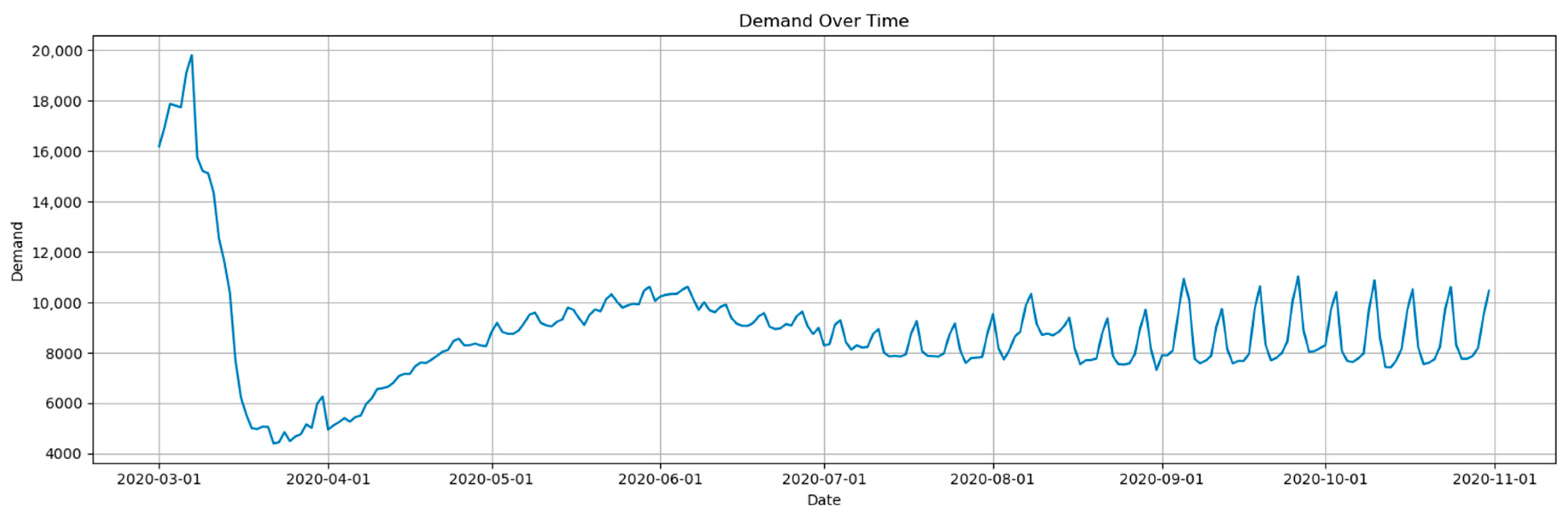
• Dataset 1: This dataset, sourced from COVID-19-related sales data, highlights volatile sales dynamics caused by pandemic-induced consumer behavior changes. It includes 13 features, such as the date, sales, and region, reflecting the impact of lockdown measures and recovery phases on sales.
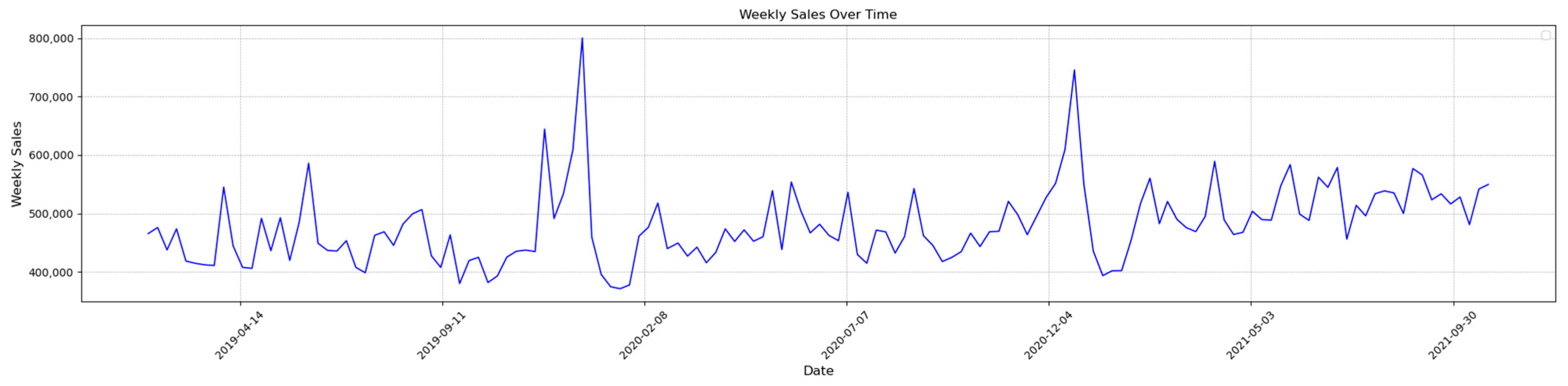
• Dataset 2: This dataset provides weekly Walmart sales data across multiple stores, including features like the store, weekly sales, and holiday flags. Its structure allows for an in-depth evaluation of forecasting models in a multi-regional retail context, making it ideal for testing the adaptability of the proposed algorithms.
• Dataset 3: Focused on Amazon UK sales, this dataset spans from 2019 to 2021 and includes 21 features, such as the weekly sales, product category, and promotional discounts. Its temporal coverage captures critical patterns in e-commerce growth during the pandemic era.

The datasets in this study, illustrated in Figure 1, Figure 2 and Figure 3 and summarized in

Table 1. The datasets used in the experiments.

Dataset	Source	No. of Instances	No. of Features
Dataset 1	https://github.com/ashfarhangi/COVID-19/ (accessed on 8 October 2024)	30,264	13
Dataset 2	https://www.kaggle.com/datasets/aslanahmedov/walmart-sales-forecast (accessed on 8 October 2024)	8190	12
Dataset 3	https://data.world/revanthkrishnaa/amazon-uk-sales-forecasting-2018-2021/workspace/project-summary (accessed on 8 October 2024)	8661	21

, capture a range of sales dynamics with varying temporal patterns, demand fluctuations, and feature complexities. This diversity enables a rigorous assessment of the hybrid ABC-FHO model’s performance across distinct sales environments.

3.1. Experimental Setup

All the experiments were implemented in Python 3.13.1 and executed on a 3.13 GHz PC with 16 GB RAM, running Windows 10. The performance of the proposed algorithms was validated by conducting experiments using publicly available sales datasets. The characteristics of these datasets are outlined in Table 1, including the number of features, the instances, and the dataset sources. To standardize the results, each dataset was preprocessed to handle any missing or outlier data before training, ensuring model consistency across all the trials. Each dataset was randomly divided into 80% for training and 20% for testing, with a 5-fold cross-validation applied to evaluate the model’s performance. To ensure reproducibility, a fixed random seed of 42 was used for all experiments.

3.2. Parameter Settings

The GA, ARO, the WSO, the GWO, the standalone ABC algorithm, the standalone FHO, and the hybrid ABC-FHO approaches, including both well-known and novel metaheuristics, were evaluated for their effectiveness in hyperparameter optimization. Recommended parameter values from the literature were used for all the algorithms [20,31,32,33]. Using default or recommended parameter values for metaheuristic algorithms is a widely accepted practice, as empirical studies have demonstrated their effectiveness in achieving reliable results without the need for extensive tuning [42]. The hybrid ABC-FHO method naturally inherits parameter settings from both the standalone ABC algorithm and the FHO, ensuring compatibility within a unified framework. By maintaining identical parameter values across standalone and hybrid methods, the comparison isolates the impact of hybridization itself, avoiding variations caused by parameter differences. A uniform population size of 10 and a maximum of 30 iterations were applied to all algorithms, balancing the computational efficiency with the effective performance.

Table 2. The lower and upper bounds of the hyperparameters of XGBoost.

Hyperparameters	Lower Bound	Upper Bound	Default Value
Colsample Bytree	0	1	1
N Estimators	30	1000	100
Max Depth	0	∞	6
Learning Rate	0	1	0.3
Min Child Weight	0	∞	1
Reg Alpha	0	∞	0
Reg Lambda	0	∞	1
Subsample	0	1	1
Max Leaves	0	∞	0

presents the initial range of hyperparameters for the XGBoost algorithm, encompassing a wide range to explore potential configurations. These bounds, including parameters such as the colsample bytree, n estimators, and learning rate, were designed to allow flexibility in parameter tuning and ensure a comprehensive search of the solution space. The selection and range, shown in

Table 3. The selected lower bounds and upper bounds of the search area in the case study.

Hyperparameters	Lower Bound	Upper Bound
Colsample Bytree	0.5	1
N Estimators	50	1000
Max Depth	2	15
Learning Rate	0.1	0.5
Min Child Weight	0.001	10
Reg Alpha	0	1
Reg Lambda	0	1
Subsample	0.5	1
Max Leaves	10	900

, of hyperparameters for XGBoost were informed by a thorough review of prior studies [32,43,44], emphasizing the most impactful parameters to optimize the model performance while maintaining the computational feasibility. Parameters such as the learning rate, max depth, and colsample bytree were identified for their significant contribution to enhancing the model accuracy and generalization. Additionally, certain hyperparameters with inherently large or limitless boundaries, like the max leaves, were bounded to control the tree complexity and avoid overfitting. Parameters such as the subsample and min child weight were included to introduce randomness and regulate the tree-splitting criteria, further improving the model’s robustness.

Table 3 shows the refined search range for the hyperparameters used in the case study. This focused range was selected based on initial empirical tests and prior literature studies, narrowing down the bounds to values likely to yield an optimal model performance while reducing the computational demands. This refinement ensured that the optimization process was both efficient and targeted, facilitating robust model tuning within practical time limits.

In this study, we employed the hybrid ABC-FHO approach, along with several comparison algorithms, to optimize these hyperparameters within the search space defined in Table 3. By using this comprehensive range, the algorithms can explore a wide search space, aiming to identify the optimal parameter settings that maximize the predictive accuracy of the XGBoost model. This setup allowed us to effectively evaluate the performance of the hybrid and comparison algorithms in tuning the model for an enhanced forecasting accuracy.

3.3. Evaluation Metrics

In this study, two statistical metrics were employed to assess the accuracy of the forecasting models. These metrics were the mean absolute percentage error (MAPE) and the root mean squared error (RMSE). In the following Equations (1) and (2), N represents the quantity of observations during both the training and testing phases, $y_i$ denotes the observed value, ${\hat{y}}_i$ represents the prediction, and ${\overline{y}}_i$ refers to the average of the actual values.

The MAPE calculates the average percentage error between the predicted and actual values, providing a normalized measure of accuracy.

$$\mathrm{MAPE}={\displaystyle \frac{1}{N}}{\displaystyle \sum }_{i=1}^N\left|{\displaystyle \frac{y\left(i\right)-\hat{y}\left(\mathrm{i}\right)}{y\left(i\right)}}\right|\times 100\%$$

(5)

The RMSE measures the square root of the average squared differences between the predicted and observed values, which gives more weight to larger errors.

$$\mathrm{RMSE}=\sqrt{{\displaystyle \frac{1}{N}}{\displaystyle \sum }_{i=1}^N{\left(y\left(i\right)-\hat{y}\left(\mathrm{i}\right)\right)}^2}$$

(6)

Smaller values for both metrics (MAPE and RMSE) indicate a better model performance, as they signify lower the prediction error. These metrics were computed for both the training and testing stages to ensure the robustness of the forecasting models [45,46].

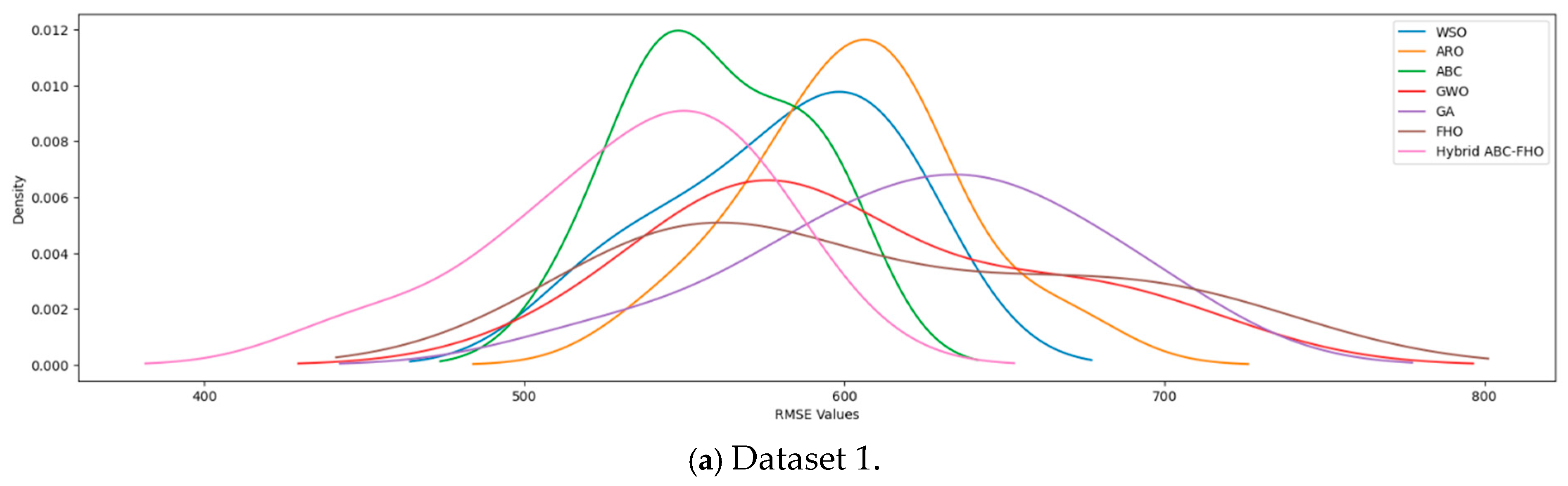
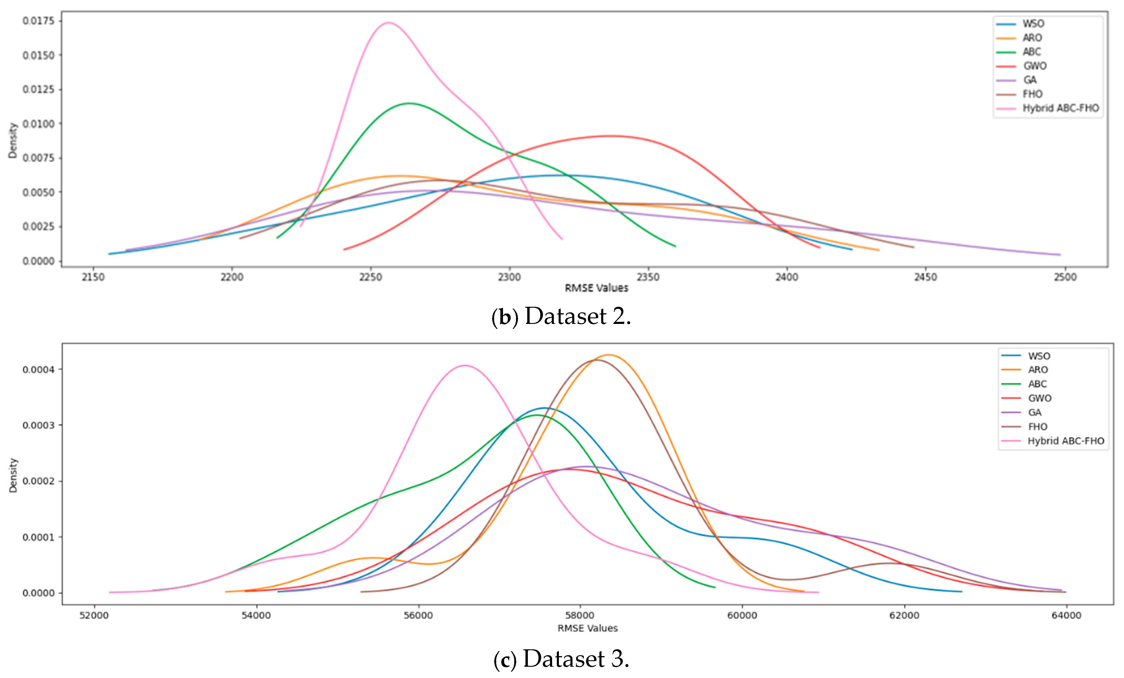
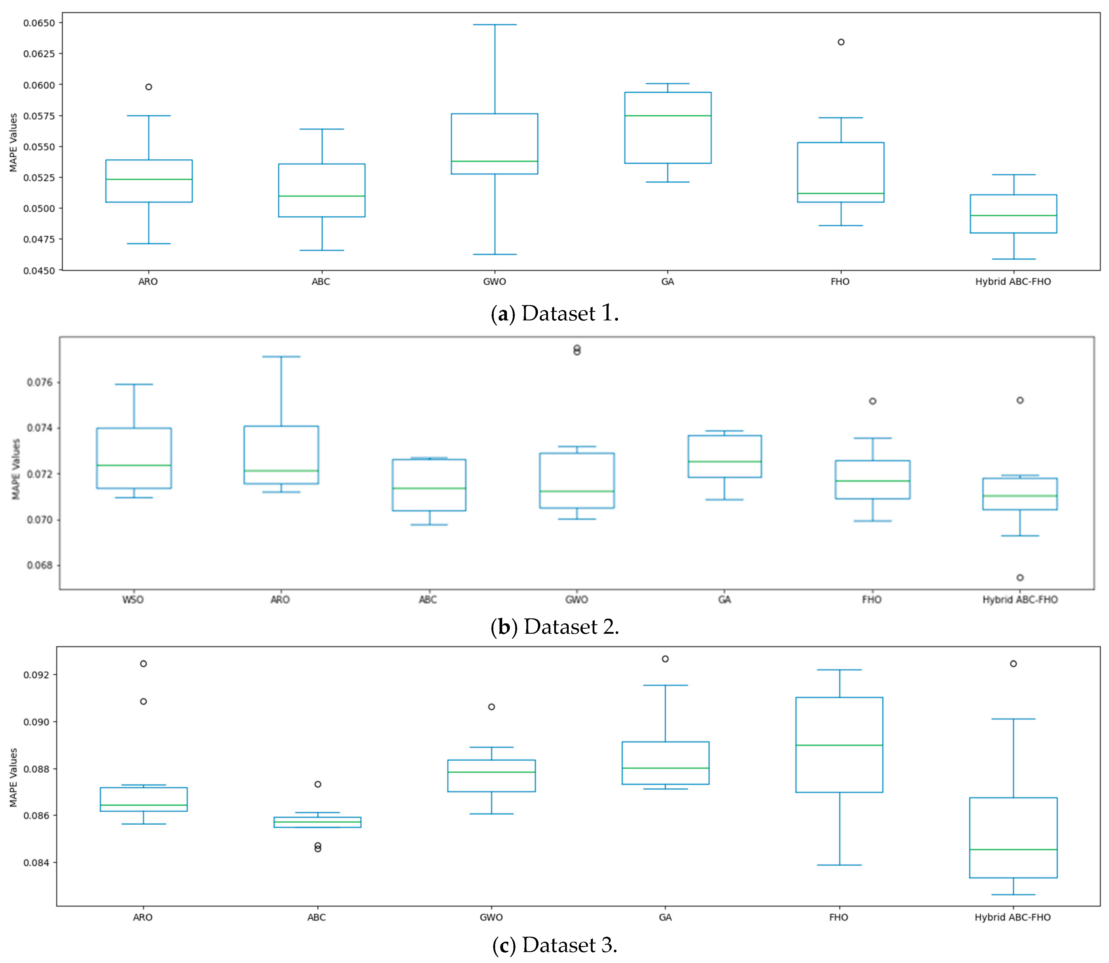
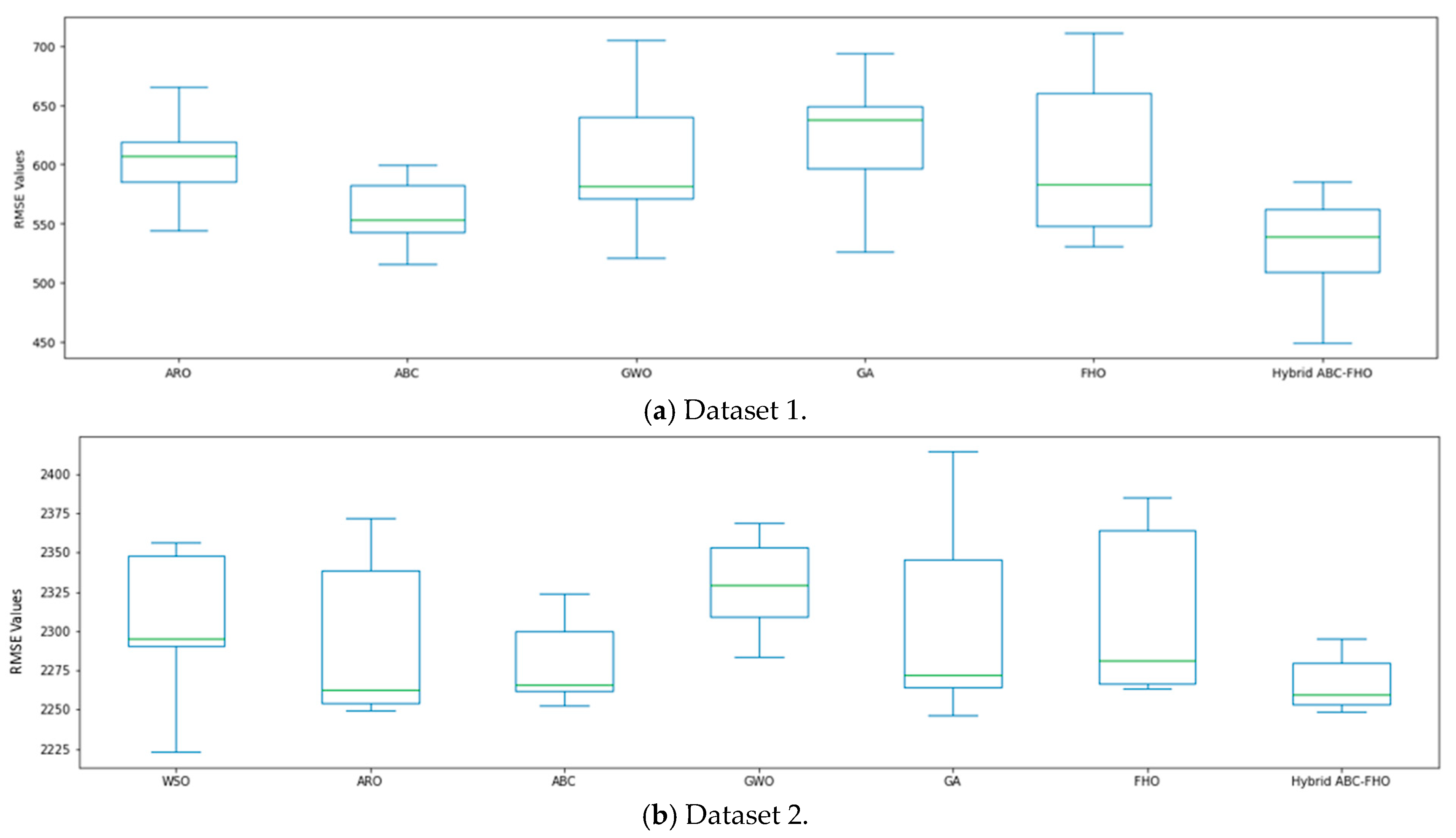
3.4. Results and Analysis

This subsection presents the performance results of the GA, ARO, the WSO, the GWO, the standalone ABC algorithm, the standalone FHO, and the hybrid ABC-FHO algorithm. The evaluation was based on the performance measurements mentioned previously, with an additional analysis of convergence behavior, box plots, and a statistical analysis.

Performance Results

The performance of the algorithms across the three sales-forecasting datasets is summarized in

Table 4. The average results for the MAPE and RMSE values of the implemented algorithms.

Dataset	Metric	GA	ARO	WSO	GWO	ABC	FHO	ABC-FHO
Dataset 1	MAPE	0.057	0.053	0.052	0.055	0.051	0.053	0.049
	RMSE	624.90	602.96	580.21	601.93	559.80	607.50	532.96
Dataset 2	MAPE	0.073	0.073	0.073	0.072	0.071	0.072	0.071
	RMSE	2308.38	2295.41	2302.68	2328.83	2296.83	2312.16	2279.23
Dataset 3	MAPE	0.0887	0.0874	0.0871	0.0878	0.0856	0.0887	0.0855
	RMSE	58,878.51	57,974.10	58,054.78	58,578.09	56,733.30	58,564.27	56,614.05

,

Table 5. The best and worst results for the MAPE values of the implemented algorithms.

Dataset		Metric	GA	ARO	WSO	GWO	ABC	FHO	ABC-FHO
Dataset 1	Best	MAPE	0.052	0.047	0.045	0.046	0.047	0.049	0.046
	Worst	MAPE	0.060	0.060	0.059	0.065	0.056	0.063	0.053
Dataset 2	Best	MAPE	0.072	0.071	0.070	0.070	0.070	0.070	0.068
	Worst	MAPE	0.075	0.077	0.075	0.077	0.073	0.074	0.074
Dataset 3	Best	MAPE	0.0968	0.0975	0.0908	0.0943	0.0958	0.0929	0.0920
	Worst	MAPE	0.1048	0.1045	0.1061	0.1043	0.1000	0.1028	0.0985

and

Table 6. The best and worst results for the RMSE values of the implemented algorithms.

Dataset		Metric	GA	ARO	WSO	GWO	ABC	FHO	ABC-FHO
Dataset 1	Best	RMSE	527.4	484.9	540.5	470.0	482.1	485.1	475.1
	Worst	RMSE	714.91	716.40	692.78	724.93	689.39	663.79	638.41
Dataset 2	Best	RMSE	2246.1	2249.8	2222.7	2283.3	2280.8	2263.6	2267.2
	Worst	RMSE	2414.2	2338.4	2356.4	2368.9	2323.9	2384.9	2295.4
Dataset 3	Best	RMSE	56,740.1	55,407.8	56,378.2	56,323.6	54,457.2	57,468.1	54,375.3
	Worst	RMSE	61,537.1	58,974.6	60,597.3	61,244.5	57,925.9	61,815.3	58,751.6

. Each algorithm was executed 10 times independently to ensure reliable conclusions. The RMSE and MAPE were the primary metrics used, given the focus on regression tasks.

Table 4 displays the average mean absolute percentage error (MAPE) and root mean squared error (RMSE) values obtained by each algorithm across the three sales-forecasting datasets. The values represent the average of 10 independent runs to ensure reliability. Lower MAPE and RMSE values indicate a better model accuracy, with the hybrid ABC-FHO algorithm consistently achieving the lowest error metrics across all the datasets. The bolded values highlight the best-performing algorithm for each metric.

For Dataset 1, the hybrid ABC-FHO algorithm achieved the lowest MAPE (0.049) and RMSE (532.96), outperforming the other algorithms by a noticeable margin, particularly when compared to the GA and the GWO, which recorded the highest RMSE values. In Dataset 2, the error values were relatively close across algorithms, yet the ABC-FHO algorithm maintained a slight edge, with an MAPE of 0.071 and an RMSE of 2279.23, showing its robustness in various forecasting contexts. Similarly, for Dataset 3, the ABC-FHO algorithm again demonstrated a superior performance, with the lowest RMSE (56614.05) scores.

Table 5 shows the best and worst MAPE values recorded for each algorithm across the three datasets, providing insights into both their peak performance and their variability. The best-case MAPE values illustrate each algorithm’s optimal accuracy, while the worst-case values highlight performance consistency and resilience under varying conditions.

Table 6 presents the best and worst RMSE values for each algorithm across the three datasets, providing insights into their accuracy and consistency. The best RMSE values represent the optimal predictive accuracy achieved, while the worst RMSE values indicate variability across runs, reflecting each algorithm’s stability.

Figure 4 and Figure 5 show the distribution of the MAPE and RMSE values, respectively, across 10 independent runs for each algorithm in Datasets 1, 2, and 3. The density curves highlight each algorithm’s performance consistency, with narrower distributions indicating more stable and reliable results. Variations in the spread across the datasets reveal how each algorithm responds to different data characteristics, providing insight into their robustness and adaptability.

As shown in Figure 4, the hybrid ABC-FHO algorithm generally exhibited narrower and more concentrated distributions across all the datasets compared to the other algorithms, indicating a consistent accuracy with minimal performance variation. This is particularly noticeable in Dataset 1, where the ABC-FHO algorithm’s density curve was tightly centered around lower MAPE values, suggesting a high stability and reliability. Datasets 2 and 3 showed a similar trend, with the ABC-FHO algorithm maintaining one of the more stable distributions, although the overall spread was broader due to dataset complexity.

Figure 5 (RMSE distributions) further supports these observations. The ABC-FHO algorithm displayed one of the narrower distributions across all the datasets, particularly in Dataset 1, where it achieved consistently low RMSE values. In Datasets 2 and 3, the ABC-FHO algorithm continued to exhibit a comparatively stable performance, with a reduced spread that indicated resilience in achieving accurate predictions, despite variations in the data characteristics.

Figure 6 and Figure 7 display the box plots of MAPE and RMSE values across multiple runs for each algorithm on Datasets 1, 2, and 3. These plots offer insights into the accuracy and stability of each algorithm. The algorithms with narrower interquartile ranges and fewer outliers exhibited a more consistent performance, while those with wider distributions indicate a higher variability. The box plots highlight how each algorithm’s performance fluctuated across datasets, suggesting differing levels of sensitivity to data characteristics and initial conditions. This variation in the spread across the MAPE and RMSE values reflects each algorithm’s robustness and reliability in handling diverse forecasting scenarios.

The algorithms with narrower interquartile ranges and fewer outliers demonstrated a greater consistency. As shown in Figure 6 and Figure 7, the hybrid ABC-FHO algorithm, in particular, exhibited narrower spreads and fewer outliers in both the MAPE and RMSE across datasets, indicating a reliable and stable performance. This consistency suggests that the ABC-FHO algorithm is less sensitive to data variability and initial conditions, making it a robust choice for diverse forecasting scenarios.

Table 7. The average results for the time duration values of the implemented algorithms.

Dataset	GA	ARO	WSO	GWO	ABC	FHO	ABC-FHO
Dataset 1	15.882	16.677	15.275	11.694	21.536	17.110	23.442
Dataset 2	45.413	48.612	45.193	48.987	60.380	41.552	68.350
Dataset 3	18.190	18.068	17.379	16.512	20.440	16.256	22.130

shows the average time duration, measured in seconds, required by each algorithm to complete the forecasting tasks across the three datasets. The hybrid ABC-FHO algorithm exhibited longer computation times compared to the standalone approaches, especially for Dataset 2. However, this trade-off is justified by the superior predictive accuracy it provides. The standalone GWO algorithm was the fastest across all the datasets, making it a suitable choice for scenarios where computational efficiency is critical.

To validate the robustness and superiority of the hybrid ABC-FHO algorithm, a rigorous statistical analysis was conducted. As described in the Experimental Setup, all the algorithms, including the ABC-FHO algorithm, were executed under a consistent setup of 10 agents and 20 iterations, repeated 10 times independently. This setup ensured the collection of reliable performance metrics, including the MAPE and RMSE, across multiple datasets. These repeated runs provided the basis for assessing the variability and statistical significance of performance differences.

First, the Shapiro–Wilk test was applied to examine whether the distributions of the MAPE and RMSE values for each algorithm followed a normal distribution. The null hypothesis for this test stated that the data are normally distributed. The results, however, indicated non-normal distributions across all the datasets, necessitating the use of a non-parametric test for further analysis. This step was critical to ensure the appropriateness of subsequent statistical methods.

To compare the ABC-FHO algorithm’s performance with other algorithms, the Mann–Whitney U test was employed as a robust non-parametric statistical method. The null hypothesis for this test assumed no significant difference between the performance of the ABC-FHO algorithm and each of the other algorithms. Rejecting the null hypothesis indicates that the observed differences are statistically significant and not due to random variation. The Mann–Whitney U test was applied to both the MAPE and RMSE values, ensuring a comprehensive evaluation of algorithm performance.

The results of the Mann–Whitney U test, presented in

Table 8. Hypothesis testing results (MAPE and RMSE) for the ABC-FHO and benchmark algorithms across datasets.

Dataset	Algorithms	Hypothesis (MAPE)	Hypothesis (RMSE)
Dataset 1	GA	Rejected	Rejected
	ARO	Rejected	Rejected
	WSO	Rejected	Rejected
	GWO	Rejected	Rejected
	ABC	Rejected	Not Rejected
	FHO	Rejected	Rejected
Dataset 2	GA	Rejected	Rejected
	ARO	Rejected	Rejected
	WSO	Rejected	Rejected
	GWO	Not Rejected	Rejected
	ABC	Not Rejected	Rejected
	FHO	Rejected	Rejected
Dataset 3	GA	Rejected	Rejected
	ARO	Rejected	Rejected
	WSO	Rejected	Rejected
	GWO	Rejected	Rejected
	ABC	Rejected	Rejected
	FHO	Rejected	Rejected

, reveal that the null hypothesis was rejected for the ABC-FHO algorithm in most cases across the datasets. This indicates that the ABC-FHO algorithm’s performance improvements in both the MAPE and RMSE were statistically significant when compared to those of other algorithms. These findings demonstrate that the hybrid ABC-FHO algorithm consistently outperformed the standalone and other hybrid algorithms, providing strong statistical evidence of its robustness and effectiveness.

By combining the results of the Shapiro–Wilk and Mann–Whitney U tests, the analysis conclusively validated that the success of the ABC-FHO algorithm was not coincidental. Instead, its superior performance can be attributed to the effective integration of the strengths of the ABC algorithm and the FHO, further underscoring the benefits of the hybridization approach.

In our experiments, conducted on three different sales datasets, the hybrid ABC-FHO algorithm consistently outperformed the other tested methods, including the standalone GA, ARO, the WSO, the ABC algorithm, and the FHO. Notably, this is the first time that the FHO has been applied as a standalone method in hyperparameter optimization, and it showed promising results. To ensure the reliability of our findings, we applied cross-validation and ran each model 10 times. The results were then averaged, and statistical tests were performed. These tests confirmed that the performance improvements brought by our hybrid approach were statistically significant. However, while the hybrid model excelled in prediction accuracy, it had the longest computational time among all the algorithms. In contrast, the standalone GWO was the fastest in terms of its computational performance.

4. Conclusions and Future Work

This study investigated the effectiveness of various metaheuristic algorithms in optimizing hyperparameters for machine learning models, with a specific focus on the hybrid ABC-FHO approach. Sales forecasting, as demonstrated, plays a crucial role in strategic decision-making within industries by enhancing the operational efficiency, inventory management, and revenue optimization. In comparing multiple algorithms, including the GA, ARO, the WSO, the GWO, the ABC algorithm, and the FHO, the hybrid ABC-FHO algorithm consistently emerged as a top performer across key metrics such as the mean absolute percentage error (MAPE) and root mean squared error (RMSE). This superior performance highlights the ABC-FHO algorithm’s capability of handling complex and nonlinear sales data across diverse datasets, including hotel demand, Walmart, and Amazon datasets, each with unique characteristics in terms of their features and data volume.

The hybrid ABC-FHO algorithm demonstrated an effective balance between exploration and exploitation, leveraging the strengths of both the artificial bee colony (ABC) and fire hawk optimizer (FHO) algorithms. This synergy contributed to an improved search efficiency, enabling the ABC-FHO algorithm to navigate high-dimensional hyperparameter spaces and deliver lower error rates. By achieving lower MAPE and RMSE values, the ABC-FHO algorithm proved its robustness and adaptability in handling a variety of dataset complexities, suggesting its suitability for real-world applications where data patterns and forecasting requirements vary widely.

However, this study also revealed a trade-off between accuracy and computational efficiency. While the ABC-FHO algorithm delivered the best predictive accuracy, it required more computational time compared to standalone algorithms such as the GWO, which demonstrated the fastest runtime across all datasets. This trade-off suggests that, while the ABC-FHO algorithm is suitable for tasks prioritizing accuracy, such as long-term forecasting or high-stakes decisions, it may be less ideal for real-time or time-sensitive applications where computational speed is crucial. Future work could focus on addressing this limitation by exploring parallel computing techniques or adaptive population management strategies to reduce the runtime without compromising the accuracy, thereby making the algorithm more practical for a wider range of applications.

To further enhance the understanding of the ABC-FHO algorithm’s capabilities, future research should explore its application across diverse datasets and industries, validating its generalizability. The hybrid approach could also be applied to other machine learning algorithms and forecasting domains, such as customer churn predictions and demand forecasting, to evaluate its adaptability beyond sales forecasting.

In summary, the hybrid ABC-FHO algorithm presents a robust solution for hyperparameter optimization in sales forecasting, effectively balancing the predictive accuracy with the computational demands. This study’s findings underscore the importance of hybrid algorithms in achieving reliable results for complex forecasting tasks, where data variability and model accuracy are paramount. The ABC-FHO algorithm’s performance supports its application in diverse forecasting contexts, providing a promising approach for industries aiming to enhance their predictive capabilities amidst varying data complexities and operational requirements.

References

1. Huber, J.; Stuckenschmidt, H. Advances in seasonal and promotional sales forecasting using machine learning models. J. Bus. Res. 2020, 117, 452–461. [Google Scholar] [CrossRef]
2. Choi, Y.; Seo, S.; Lee, J.; Kim, T.W.; Koo, C. A machine learning-based forecasting model for personal maximum allowable exposure time under extremely hot environments. Sustain. Cities Soc. 2024, 101, 105140. [Google Scholar] [CrossRef]
3. Singh, A.R.; Kumar, R.S.; Bajaj, M.; Khadse, C.B.; Zaitsev, I. Machine learning-based energy management and power forecasting in grid-connected microgrids with multiple distributed energy sources. Sci. Rep. 2024, 14, 19207. [Google Scholar] [CrossRef]
4. Zhang, X.; Liu, X.; Wang, X.; Band, S.S.; Bagherzadeh, S.A.; Taherifar, S.; Abdollahi, A.; Bahrami, M.; Karimipour, A.; Chau, K.-W.; et al. Energetic thermo-physical analysis of MLP-RBF feed-forward neural network compared with RLS fuzzy to predict CuO/liquid paraffin mixture properties. Eng. Appl. Comput. Fluid Mech. 2022, 16, 764–779. [Google Scholar] [CrossRef]
5. Ben Jabeur, H.; Bouzidi, M.; Malek, J. XGBoost outperforms traditional machine learning models in retail demand forecasting. J. Retail. Consum. Serv. 2024, 67, 102859. [Google Scholar]
6. Mishra, P.K.; Singh, S.; Kumar, A.; Gupta, V. Evaluating the performance of machine learning models in rainfall forecasting: A comparison of XGBoost, ARIMA, and state space models. Environ. Earth Sci. 2024, 83, 11481. [Google Scholar] [CrossRef]
7. Zhang, X.; Wu, Y.; Li, Z. A comparison of XGBoost and ARIMA in demand forecasting of e-commerce platforms. Electron. Commer. Res. Appl. 2021, 45, 101030. [Google Scholar]
8. Massaro, M.; Dumay, J.; Garlatti, A. A hybrid XGBoost-ARIMA model for improving sales forecasting accuracy in retail. J. Bus. Econ. Manag. 2021, 22, 512–526. [Google Scholar]
9. Panarese, P.; Vasile, G.; Zambon, E. Sales forecasting using XGBoost: A case study in the e-commerce sector. Expert Syst. Appl. 2021, 177, 114934. [Google Scholar] [CrossRef]
10. Arnold, C.; Biedebach, L.; Küpfer, A.; Neunhoeffer, M. The role of hyperparameters in machine learning models and how to tune them. Political Sci. Res. Methods 2024, 12, 841–848. [Google Scholar] [CrossRef]
11. Ali, A.; Zain, A.M.; Zainuddin, Z.M.; Ghani, J.A. A survey of swarm intelligence and evolutionary algorithms for hyperparameter tuning in machine learning models. Swarm Evol. Comput. 2023, 56, 100–114. [Google Scholar]
12. Tani, L.; Rand, D.; Veelken, C.; Kadastik, M. Evolutionary algorithms for hyperparameter optimization in machine learning for application in high energy physics. Eur. Phys. J. C 2021, 81, 170. [Google Scholar] [CrossRef]
13. Yin, X.; Cheng, S.; Yu, H.; Pan, Y.; Liu, Q.; Huang, X.; Gao, F.; Jing, G. Probabilistic assessment of rockburst risk in TBM-excavated tunnels with multi-source data fusion. Tunn. Undergr. Space Technol. 2024, 152, 105915. [Google Scholar] [CrossRef]
14. Du, X.; Xu, H.; Zhu, F. Understanding the effect of hyperparameter optimization on machine learning models for structure design problems. Comput. Aided Des. 2021, 135, 103013. [Google Scholar] [CrossRef]
15. Dhake, P.S.; Patil, A.D.; Desai, R.R. Genetic algorithm for optimizing hyperparameters in LSTM-based solar energy forecasting. Renew. Energy 2023, 198, 75–84. [Google Scholar] [CrossRef]
16. Zulfiqar, U.; Rehman, M.U.; Khan, A. Adaptive differential evolution and support vector machines for load forecasting. Electr. Power Syst. Res. 2022, 208, 107976. [Google Scholar] [CrossRef]
17. Kaya, E.; Gorkemli, B.; Akay, B.; Karaboga, D. A review on the studies employing artificial bee colony algorithm to solve combinatorial optimization problems. Eng. Appl. Artif. Intell. 2022, 115, 105311. [Google Scholar] [CrossRef]
18. Mohakud, B.; Dash, R. Grey wolf optimization-based convolutional neural network for skin cancer detection. J. King Saud Univ. Comput. Inf. Sci. 2021, 34, 3717–3729. [Google Scholar] [CrossRef]
19. Tran, Q.A.; Nguyen, D.K.; Le, T.H. Enhancing long-term meteorological predictions with genetic algorithms and LSTM networks. IEEE Access 2020, 8, 29832–29843. [Google Scholar]
20. Azizi, M.; Talatahari, S.; Gandomi, A.H. Fire Hawk Optimizer: A novel metaheuristic algorithm. Artif. Intell. Rev. 2023, 56, 287–363. [Google Scholar] [CrossRef]
21. Çetinbaş, M.; Özcan, E.; Bayramoğlu, S. Hybrid White Shark Optimizer and Artificial Rabbits Optimization for photovoltaic parameter extraction. Renew. Energy 2023, 180, 1236–1249. [Google Scholar] [CrossRef]
22. Al-Shourbaji, I.; Hassan, M.M.; Mohamed, M.A. Hybrid ant colony optimization and reptile search algorithm for solving complex optimization problems. Expert Syst. Appl. 2022, 192, 116331. [Google Scholar]
23. Bindu, M.G.; Sabu, M.K. A hybrid feature selection approach using artificial bee colony and genetic algorithm. In Proceedings of the IEEE International Conference on Electronics, Computing and Communication Technologies (CONECCT), Bangalore, India, 2–4 July 2020; pp. 1–6. [Google Scholar]
24. Abd Elaziz, M.; Hosseinzadeh, M.; Elsheikh, A.H. A novel hybrid of Fire Hawk Optimizer and Artificial Rabbits Optimization for complex optimization problems. J. Intell. Fuzzy Syst. 2023, 36, 125–139. [Google Scholar] [CrossRef]
25. Abbasimehr, H.; Shabani, M.; Yousefi, M. A novel hybrid machine learning model to forecast electricity prices using XGBoost, ELM, and LSTM. Energy 2023, 263, 125546. [Google Scholar] [CrossRef]
26. Deng, Y.; Zhang, J.; Liu, F. A hybrid model of XGBoost and LSTM for electricity load forecasting. J. Energy Storage 2022, 46, 103568. [Google Scholar] [CrossRef]
27. Holland, J.H. Adaptation in Natural and Artificial Systems: An Introductory Analysis with Applications to Biology, Control, and Artificial Intelligence, 2nd ed.; MIT Press: Cambridge, MA, USA, 1992. [Google Scholar]
28. Katoch, S.; Chauhan, S.S.; Kumar, V. A review on genetic algorithm: Past, present, and future. Multimed. Tools Appl. 2021, 80, 8091–8126. [Google Scholar] [CrossRef] [PubMed]
29. Mirjalili, S.; Mirjalili, S.M.; Lewis, A. Grey wolf optimizer. Adv. Eng. Softw. 2024, 69, 46–61. [Google Scholar] [CrossRef]
30. Makhadmeh, Z.; Al Momani, M.; Mohammed, A. An enhanced Grey Wolf Optimizer for solving real-world optimization problems. Expert Syst. Appl. 2023, 213, 118834. [Google Scholar]
31. Braik, M.; Awadallah, M.A.; Mousa, A. White Shark Optimizer: A novel meta-heuristic algorithm for global optimization problems. Appl. Soft Comput. 2022, 110, 107625. [Google Scholar] [CrossRef]
32. Wang, Y.; Ni, X.S. A XGBoost risk model via feature selection and Bayesian hyper-parameter optimization. arXiv 2019, arXiv:1901.08433. [Google Scholar] [CrossRef]
33. Karaboga, D.; Basturk, B. A powerful and efficient algorithm for numerical function optimization: Artificial bee colony (ABC) algorithm. J. Glob. Optim. 2007, 39, 459–471. [Google Scholar] [CrossRef]
34. Kaya, M.; Karaboga, D.; Basturk, B. A comprehensive review of artificial bee colony algorithm variants and their applications. Swarm Evol. Comput. 2022, 72, 101069. [Google Scholar] [CrossRef]
35. Jahangir, H.; Eidgahe, D.R. A new and robust hybrid artificial bee colony algorithm—ANN model for FRP-concrete bond strength evaluation. Constr. Build. Mater. 2020, 264, 113160. [Google Scholar]
36. Lee, W.W.; Hashim, M.R. A hybrid algorithm based on artificial bee colony and artificial rabbits optimization for solving economic dispatch problem. In Proceedings of the 2023 IEEE International Conference on Automatic Control and Intelligent Systems (I2CACIS), Shah Alam, Malaysia, 17 June 2023; pp. 298–303. [Google Scholar] [CrossRef]
37. Moosavi, S.K.R.; Saadat, A.; Abaid, Z.; Ni, W.; Li, K.; Guizani, M. Feature selection based on dataset variance optimization using Hybrid Sine Cosine—Firehawk Algorithm (HSCFHA). Future Gener. Comput. Syst. 2024, 141, 1–15. [Google Scholar] [CrossRef]
38. Shapiro, S.S.; Wilk, M.B. An analysis of variance test for normality (complete samples). Biometrika 1965, 52, 591–611. [Google Scholar] [CrossRef]
39. Jurečková, J.; Picek, J. Robust Statistical Methods with R; Springer: Berlin/Heidelberg, Germany, 2007. [Google Scholar]
40. MacFarland, T.W.; Yates, J.M. Introduction to Nonparametric Statistics for the Biological Sciences Using R; Springer: Berlin/Heidelberg, Germany, 2016. [Google Scholar] [CrossRef]
41. Mann, H.B.; Whitney, D.R. On a test of whether one of two random variables is stochastically larger than the other. Ann. Math. Stat. 1947, 18, 50–60. [Google Scholar] [CrossRef]
42. Arcuri, A.; Fraser, G. Parameter tuning or default values? An empirical investigation in search-based software engineering. Empir. Softw. Eng. 2023, 18, 594–623. [Google Scholar] [CrossRef]
43. Kapoor, S.; Perrone, V. A simple and fast baseline for tuning large XGBoost models. arXiv 2021, arXiv:2111.06924. [Google Scholar] [CrossRef]
44. Kavzoglu, T.; Teke, A. Advanced hyperparameter optimization for improved spatial prediction of shallow landslides using extreme gradient boosting (XGBoost). Bull. Eng. Geol. Environ. 2022, 81. [Google Scholar] [CrossRef]
45. Tao, M.; Hong, Z.; Liu, L.; Zhao, M.; Wu, C. An intelligent approach for predicting overbreak in underground blasting operation based on an optimized XGBoost model. Eng. Appl. Artif. Intell. 2023, 6, 100279. [Google Scholar]
46. Vivas, E.; Allende-Cid, H.; Salas, R. A systematic review of statistical and machine learning methods for electrical power forecasting with reported MAPE score. Entropy 2020, 22, 1412. [Google Scholar] [CrossRef] [PubMed]
Figure 1. Dataset 1 sales graph.
Mathematics 12 03921 g001
Figure 2. Dataset 2 sales graph.
Mathematics 12 03921 g002
Figure 3. Dataset 3 sales graph.
Mathematics 12 03921 g003
Figure 4. The distribution of the MAPE values across iterations.
Mathematics 12 03921 g004
Figure 5. The distribution of the RMSE values across iterations.
Mathematics 12 03921 g005aMathematics 12 03921 g005b
Figure 6. Box plots of the MAPE values across iterations.
Mathematics 12 03921 g006
Figure 7. Box plots of the RMSE values across iterations.
Mathematics 12 03921 g007aMathematics 12 03921 g007b