A Novel DV-Hop Localization Method Based on Hybrid Improved Weighted Hyperbolic Strategy and Proportional Integral Derivative Search Algorithm

Abstract

As a range-free localization algorithm, DV-Hop has gained widespread attention due to its advantages of simplicity and ease of implementation. However, this algorithm also has some defects, such as poor localization accuracy and vulnerability to network topology. This paper presents a comprehensive analysis of the factors contributing to the inaccuracy of the DV-Hop algorithm. An improved proportional integral derivative (PID) search algorithm (PSA) DV-Hop hybrid localization algorithm based on weighted hyperbola (IPSA-DV-Hop) is proposed. Firstly, the first hop distance refinement is employed to rectify the received signal strength indicator (RSSI). In order to replace the original least squares solution, a weighted hyperbolic algorithm based on the degree of covariance is adopted. Secondly, the localization error is further reduced by employing the improved PSA. In addition, the selection process of the node set is optimized using progressive sample consensus (PROSAC) followed by a 3D hyperbolic algorithm based on coplanarity. This approach effectively reduces the computational error associated with the hopping distance of the beacon nodes in the 3D scenarios. Finally, the simulation experiments demonstrate that the proposed algorithm can markedly enhance the localization precision in both isotropic and anisotropic networks and reduce the localization error by a minimum of 30% in comparison to the classical DV-Hop. Additionally, it also exhibits stability under the influence of a radio irregular model (RIM).

1. Introduction

Wireless sensor networks (WSNs), a specialized form of wireless network organization, are widely applied in various fields. These networks consist of numerous energy-limited, low-power, and small-sized sensor nodes that are deployed to sense the surrounding environment and acquire information [1]. The primary research areas in WSNs include localization techniques, time synchronization, routing protocols, topology control, coverage control, etc. After deploying a WSN system, the first challenge is node localization in most scenarios [2].

A global positioning system (GPS) can provide location data. However, the drawbacks of GPS, including high power consumption and vulnerability to external factors, have prompted investigations of alternative methods for locating unknown nodes [3]. According to the necessity of Euclidean distances between nodes, WSN localization algorithms can be categorized as range-based and range-free. Range-based localization algorithms require additional hardware support, making them less suitable for low-power, low-cost WSN applications [4]. In contrast, range-free localization algorithms estimate node positions according to network information, such as topological relationships between nodes [5]. Therefore, this approach offers better performance in terms of hardware cost and energy consumption.

The DV-Hop algorithm is a classic range-free localization method. Its core mechanism is based on distance vector routing. With advantages such as low communication overhead and ease of deployment, it demonstrates significant potential for application in various scenarios. Currently, the majority of research on DV-Hop is concentrated on integrating novel algorithms to enhance performance during specific phases of the original DV-Hop process.

Yuxiao Cao et al. proposed an improved DV-Hop algorithm based on node negotiation and multiple communication radii. This method utilized a variable communication radius for refinement and considered only the beacon node with the least number of hops for computation, thereby improving localization accuracy [6]. In order to further enhance localization accuracy, Achroufene, A. et al. introduced a power function interpolation-based approach to rectify the RSSI values and substitute the least squares estimation with a disk-based multiplication algorithm [7]. Since WSNs are often deployed in complex terrain, many scholars have proposed DV-Hop algorithms for 3D scenarios. Singh, P. et al. proposed a swarm intelligent localization algorithm based on hybrid gray wolves and fireflies to assist localization with the assistance of virtual beacon nodes, which improved localization accuracy in 3D scenarios [8]. Mohanta, T.K. et al. achieved significant improvement in localization errors in 3D scenarios by correcting hop distances with correction factors and CTO-based orthogonal learning [9].

Although numerous improvements have been made in WSN localization, most algorithms continue to face challenges in adapting to diverse scenarios. They often suffer from complex localization processes, poor robustness, and low accuracy in various network topologies. To address these issues, a hybrid PSA-DV-Hop localization algorithm based on weighted hyperbolic improvement is proposed in this paper. In the 2D scenario, the weighted hyperbolic PSA based on collinearity can effectively improve localization accuracy while maintaining low calculation complexity. In order to extend the algorithm to 3D scenarios, the PROSAC algorithm is employed to analyze the correlation degree among nodes. In addition, the coplanarity strategy is used to correct the positions of unknown nodes. The proposed algorithm can effectively reduce the localization error in 3D scenarios.

The rest of the paper is organized as follows. Section 2 reviews the classical DV-Hop localization algorithm and analyzes the causes of errors at each stage. Section 3 introduces the principle and process of the proposed algorithm, including its extension to 3D scenarios. Algorithm performance evaluation and simulation results are shown in Section 4. Finally, Section 5 concludes this paper.

2. Related Work

2.1. Classical DV-Hop Algorithm

The classical DV-Hop algorithm estimates the location of nodes by calculating the distance between the unknown nodes and beacon nodes [10]. It can be divided into three phases:

Phase 1: Calculate the minimum hop count. Beacon nodes broadcast the packet, containing their location and hop count, to their neighbor nodes $\left(ID, x_i, y_i, hop{s}_i\right)$. The hop count value is increased by 1 at each hop. This process continues until all nodes record their minimum hop count and the coordinates of the beacon nodes [11].

Phase 2: Calculate the average hop distance among nodes. The beacon node receives data frames from other beacon nodes, stores their coordinates and hop count information, and then forwards the frames. The average hop distance can be calculated by Equation (1).

$$Hopsiz{e}_i={\displaystyle \frac{{\sum }_{i\ne j}^n\sqrt{{\left(x_i-x_j\right)}^2+{\left(y_i-y_j\right)}^2}}{{\sum }_{i\ne j}^n{H}_{ij}}}$$

(1)

where $Hopsiz{e}_i$ represents the average hop distance of beacon node $i$. $\left(x_i, y_i\right)$ and $\left(x_j, y_j\right)$ represent the coordinates of beacon nodes $i$ and $j$. $H_{ij}$ represents the minimum number of hops between beacon nodes $i$ and $j$. $n$ represents the number of beacon nodes. The unknown node calculates the distance to the beacon node based on the number of hops and the average hop distance among all the beacon nodes, which can be calculated by Equation (2).

$$d_{iu}=Hopsiz{e}_i\times H_{iu}$$

(2)

where $d_{iu}$ represents the distance between the beacon node $i$ and the unknown node $u$, and $H_{iu}$ represents the minimum number of hops between beacon node $i$ and unknown node $u$.

Phase 3: Calculate coordinates using the least squares method. After the previous two phases, the unknown nodes obtain the estimated distances to all beacon nodes. The system of linear equations can be constructed as expressed in Equation (3).

$$\left\{\begin{array}{c}(x_u-x_1{)}^2+(y_u-y_1{)}^2=d_{1u}^2\\ (x_u-x_2{)}^2+(y_u-y_2{)}^2=d_{2u}^2\\ \begin{array}{ccc}& ⋮& \begin{array}{cc}& \end{array}\end{array}\\ (x_u-x_n{)}^2+(y_u-y_n{)}^2=d_{nu}^2\end{array}\right.$$

(3)

where $\left(x_1, y_1\right)$, $\left(x_2, y_2\right)$, …, $\left(x_n, y_n\right)$ represent the coordinates of $n$ beacon nodes, and $\left(x_u, y_u\right)$ represents the coordinate of unknown node $u$. Rewrite Equation (3) in the form of $AX=b$. Then, the unknown node coordinates can be calculated using the least squares method [12].

2.2. DV-Hop Error Analysis

In DV-Hop, the coordinates of unknown nodes are estimated based on the number of hops and the beacon node coordinates, which often results in larger errors. There are three main factors contributing to these localization errors.

• Error in the hop value. Assume there are four neighboring nodes within the communication radius of a node. The hop value to each of the four neighboring nodes is assigned as 1, which is inconsistent with the actual situation. Therefore, there is a hop value error during the hop number acquisition stage [13].
• Average hop distance error. The average hop distance to the nearest beacon node is used to calculate the distance between the unknown node and the beacon node. Since the path between the two beacon nodes is not a straight line, the average hop distance is often smaller than the actual value.
• Coordinate estimation error. A certain amount of error inevitably arises during the node coordinate estimation stage in the distance calculation. As errors accumulate during the solution of the coordinate system equations, the final results deviate more significantly from the actual values [14].

2.3. PID Search Algorithm

The PID algorithm is a fundamental control strategy widely used in various applications. It can be categorized into two types: incremental PID control and positional PID control. The PID controller, which operates based on proportional, integral, and differential deviation, is one of the most widely utilized automatic control systems. PSA is a meta-heuristic approach designed for analog incremental PID control. The user sets the target value, and the controller continuously adjusts the system deviation to provide an output value to the actuator, thereby converging the entire system to the optimal state [15].

In a PID control system, the target value of the controlled system is denoted as $V_t$, while the actual value at time $t$ is represented as $V\left(t\right)$. The deviation in the control system at time $t$ is defined as $E\left(t\right)=V_t-V\left(t\right)$ [16]. The proportional control formula can be expressed by Equation (4):

$$P\left(t\right)=K_p\cdot E\left(t\right)+P_0$$

(4)

where $P\left(t\right)$ represents the output value of the proportional control at time $t$, and $K_p$ is the proportional coefficient, a factor used to adjust the deviation in the system. Additionally, $P_0$ is a constant introduced to prevent the output value from approaching zero.

Integral control takes into account the past states of the system being controlled, with the controller’s output being proportional to the integral of the input error signal. To eliminate steady-state errors, an integral term in the controller must be introduced. The integral control output value at time $t$ can be expressed as follows:

$$I\left(t\right)=K_i\cdot {\int }_0^{t}E\left(t\right)dt+I_0$$

(5)

where $K_i$ and $I_0$ represent the integral coefficient and the constant, respectively.

To mitigate potential instability during error regulation, an early correction signal that predicts the trend in error changes should be introduced into the system. The output value at time $t$ can be expressed as follows:

$$D\left(t\right)=K_d\cdot {\displaystyle \frac{dE\left(t\right)}{dt}}+D_0$$

(6)

where $K_d$ represents the differential coefficient. Thus, the classical PID algorithm can be expressed as follows:

$$O\left(t\right)=P\left(t\right)+I\left(t\right)+D\left(t\right)+O_0$$

(7)

where $O\left(t\right)$ is the control quantity output by the PID controller at moment $t$. $O_0$ refers to the output value of the PID controller at the initial time, which is used to compensate for the static error of the system. Its value depends on the static characteristics of the system and the control target.

In practice, only discrete data returned by the sensors are usually available. Therefore, the discretized form of the conventional PID algorithm is

$$O\left(t\right)=K_{p}E(t)+K_i{\sum }_{i=0}^{t}E\left(i\right)+K_d\left[E\left(t\right)-E\left(t-1\right)\right]$$

(8)

Incremental PID refers to the output of the digital controller as the increment of the control quantity. In this case, the incremental PID control algorithm can be expressed as follows:

$$\mathsf{\Delta }O\left(t\right)=K_p\left[E\left(t\right)-E\left(t-1\right)\right]+K_{i}E\left(t\right)+K_d\left[E\left(t\right)-2E\left(t-1\right)+E\left(t-2\right)\right]$$

(9)

The above formula shows that the incremental PID control is related to the systematic deviation at times $t$, $t-1$, and $t-2$. Since the deviation of the system will not accumulate, the stability of the control system is improved.

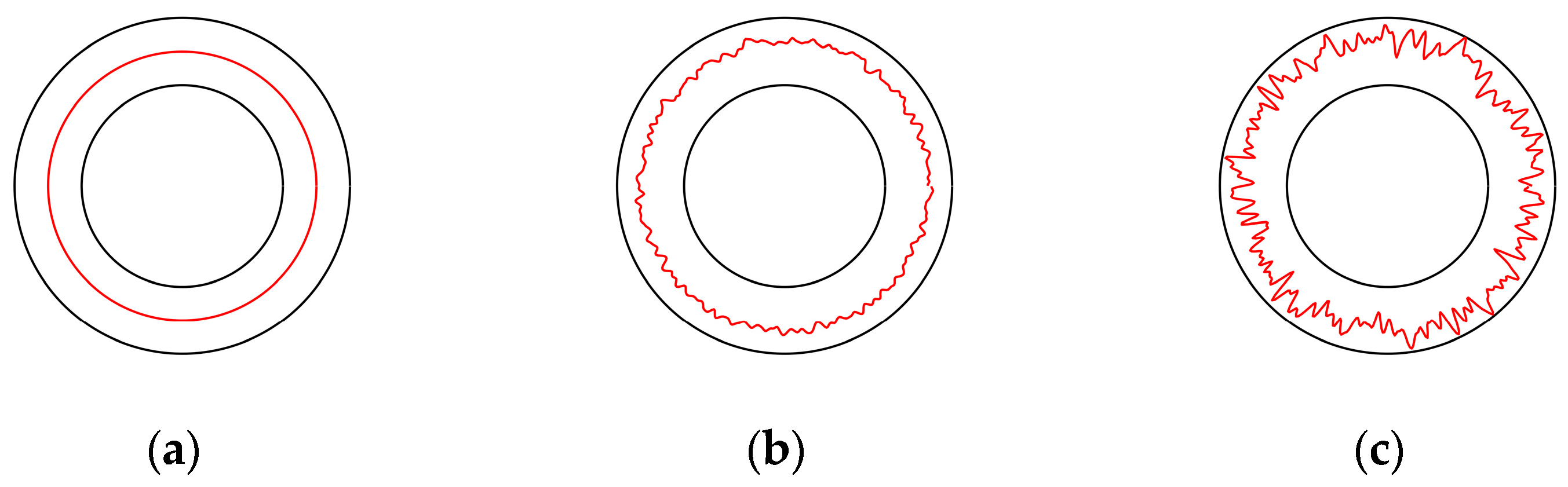
2.4. Irregular Radio Communication and Anisotropic Network

WSNs can be classified into isotropic and anisotropic networks based on their properties. The communication range of a node depends on the transmission power of the sensor node and the communication environment [17]. The incremental variation in radio signals with direction leads to irregularities in the radio direction pattern, and He Tian et al. proposed an RIM based on this characteristic [18].

The model used the degree of irregularity (DOI) to represent the percentage change in the maximum path loss per unit degree change in the direction of radio propagation. In practical scenarios, it is an irregular figure that approximates a circle. A high DOI can lead to interruptions in the communication between nodes and can alter the topological distribution of the network. Therefore, radio irregularity is one of the key factors contributing to the formation of anisotropic networks. The radiation pattern of the radio communication in different DOI states is shown in Figure 1.

3. Methodology and Model

Based on the above analysis, we improved the DV-Hop algorithm by addressing the three error sources.

3.1. IPSA-DV-Hop Algorithm

The proposed algorithm in this paper performs the first hop distance refinement during the hop count acquisition phase. In the node distance calculation phase, an improved weighted hyperbolic algorithm is adopted to replace the least squares solution. The combination of the improved DV-Hop algorithm and the optimized PSA further reduced localization error.

3.1.1. First Hop Distance Refinement and Weighting

In the algorithm, the first hop distance is refined using the RSSI, with the reference signal strength taken as the RSSI value at unit distance. The log distance path loss model can be simplified as shown in Equation (10).

$$P(d)=P(d_0)-10\eta \cdot \mathit{lg}{\displaystyle \frac{d}{d_0}}+X_{\sigma }$$

(10)

where the $P(d)$ represents the RSSI value when two nodes are $d$ meters apart. The reference distance used in the experiments in this paper is $d_0=1 \mathrm{m}$. $\eta$ is the wireless channel attenuation coefficient, which is often set to 2~4. $X_{\sigma }$ represents a Gaussian random noise.

The relationship between the distance of two nodes and the communication radius is represented by classifying the first hop into $n$ levels. The refinement grade in this paper is 3. The hierarchical classification is shown in Equation (11).

$$hops=\left\{\begin{array}{cc}{\displaystyle \frac{1}{n}},& \hfill 0<d\le {\displaystyle \frac{R}{n}}\\ {\displaystyle \frac{i}{n}},& \hfill {\displaystyle \frac{\left(i-1\right)R}{n}}<d\le {\displaystyle \frac{iR}{n}}\\ 1,& \hfill {\displaystyle \frac{\left(n-1\right)R}{n}}<d\le R\end{array}\right.$$

(11)

The relationship between distance and the RSSI can be expressed by Equation (12).

$$P\left(d_0\right)-10\eta \cdot \mathit{lg}\left({\displaystyle \frac{iR}{n}}\right)+X_{\sigma }\le P\left(d\right)<P\left(d_0\right)-10\eta \cdot \mathit{lg}\left[{\displaystyle \frac{\left(i-1\right)R}{n}}\right]+X_{\sigma }$$

(12)

The estimated distance error is used as a weighting coefficient to calculate the distance error for each beacon node, as expressed by Equation (13). The two algorithms complement each other, effectively addressing the limitations of using RSSI technology alone, such as low accuracy and susceptibility to interference.

$$e_i={\displaystyle \frac{1}{N}}{\sum }_{i\ne j}{\displaystyle \frac{\left|d_{ij}^{\prime }-d_{ij}\right|}{h_{ij}}},aveHop{s}_i={\sum }_{i=1}^n{w}_i\cdot hop{s}_i,w_i={\displaystyle \frac{e_i}{{\sum }_{j=1}^N{e}_j}}$$

(13)

3.1.2. Weighted Hyperbolic Strategy Based on Collinearity

The hyperbolic localization algorithm determines the position of the node to be localized by placing it on a hyperbola, with the beacon node as the focus and the distance between the two beacon nodes as the focal length. The $d_{ui}$ and $d_{uj}$ represent the distance from the unknown node $u$ to the beacon node $i$ and beacon node $j$, respectively. The difference between the distances of the two beacon nodes to the unknown node is $r_{ij}=d_{ui}-d_{uj}$. The coordinates of the nodes are determined from the intersection of the hyperbolas, and the hyperbola equation can be expressed by Equation (14).

$$r_{ij}+2r_{ij}\cdot d_{uj}+{d_{uj}}^2=-2x_i\cdot x-2y_i\cdot y+{x_i}^2+{y_i}^2+x^2+y^2$$

(14)

Observations with higher variance in the error term are assigned smaller weights to create a model without heteroskedasticity. The performance index can then be expressed as Equation (15):

$$\sigma \left(c\right)=[b-Ac{]}^{T}W[b-Ac]$$

(15)

where $\sigma \left(c\right)$ represents the sum of squares of deviations, and $W$ is a weighted positive definite matrix.

The estimator obtained from Equation (15) minimizes and satisfies the conditions for the optimal linear unbiased estimate. The coordinates at the extremes can be obtained by taking the partial derivative and setting it equal to zero. The estimation error at this point is

$$E\left\{\right[c-c_{\mathrm{LSW}}\left]\right[c-c_{\mathrm{LSW}}{]}^T\}={\left(AWA\right)}^{-1}{A}^{T}W{R}_{\xi }WH{\left(A^{T}WA\right)}^{-1}$$

(16)

According to the Cauchy–-Schwartz inequality, we can obtain the following:

$$E\left\{\xi {\xi }^T\right\}=diag\left(E\left\{{\xi }_1{\xi }_1\right\},E\left\{{\xi }_2{\xi }_2\right\},\cdots ,E\left\{{\xi }_n{\xi }_n\right\}\right)+B$$

(17)

When the unknown node $u$ is not collinear with nodes $i$ and $j$, the distance error between $u$ and $i$, and the distance error between $u$ and $j$, are independent of each other. According to the network distribution characteristics, the product of the variance in the error term and the corresponding weight coefficient is a constant that is independent of $i$. In this case, the heteroskedasticity more approximately satisfies the conditions for the best linear unbiased estimation.

$$E\{w_i·{\xi }_i^2\}=4w_i·{Hopsize}_u^2·h_{ui}^2·E\left\{{∆d}_{ui}^2\right\}=4{Hopsize}_u^2·{\sigma }^2$$

(18)

When the nodes are collinear, the matrix approaches a singular matrix due to the limited measurement information. The degree of collinearity (DCL) is introduced in the proposed algorithm, with values closer to 1 indicating that the group of nodes is closer to collinearity [19]. The absolute value of the cosine of the angle in the triangle is calculated using Equation (19):

$$C_a=\left|{\displaystyle \frac{\left({L_b}^2+{L_c}^2-{L_a}^2\right)}{2L_b\cdot L_c}}\right|, C_b=\left|{\displaystyle \frac{\left({L_a}^2+{L_c}^2-{L_b}^2\right)}{2L_a\cdot L_c}}\right|, C_c=\left|{\displaystyle \frac{\left({L_a}^2+{L_b}^2-{L_c}^2\right)}{2L_a\cdot L_b}}\right|$$

(19)

where $L_a$, $L_b$, and $L_c$ represent the lengths of the sides corresponding to the three angles.

The maximum value among $C_a$, $C_b$, and $C_c$ is taken as the DCL for a set of nodes. The average value is then calculated as an effective threshold for the DCL. When the DCL exceeds this threshold, the group of nodes is considered to have a large localization error and does not participate in the localization process.

Different weights are assigned to the $m$ sets of estimated coordinates of suitable nodes that perform the hyperbolic algorithm, as shown in Equation (20). The unknown node then performs weighted processing on the $m$ sets of estimated coordinates, with the result serving as the final coordinates.

$$D_i={\displaystyle \frac{\frac{1}{DC{L}_i}}{{\sum }_{i=1}^m\frac{1}{DC{L}_i}}}, W_i={\displaystyle \frac{DC{L}_i+w_i}{{\sum }_{i=1}^m\left(DC{L}_i+w_i\right)}}$$

(20)

3.1.3. Improved PSA Mechanism

The PSA requires the initialization of the population. For the localization problem, the number of decision variables is denoted as $d$, and the upper and lower bounds of the variables are $ub$ and $lb$, respectively. The control parameters of the algorithm include the maximum number of iterations $T$ and the population size $n$. Therefore, the initial population can be expressed by Equation (21):

$$x_{ij}=\left(u{b}_j-l{b}_j\right)\cdot r_1+l_j\left(i=1, 2, \cdots , n; j=1, 2, \cdots , d\right)$$

(21)

where $r_1$ is a random number from 0 to 1, and $x_{ij}$ represents the $j$-th dimension of the individual.

The fitness function for estimating the unknown node locations is constructed using the table of beacon node locations and distances between network nodes, as follows:

$$fitness(x,y)={\sum }_{i=1}^M{\left[\sqrt{{\left(x_i-x_u\right)}^2+{\left(y_i-y_u\right)}^2}-d_{iu}\right]}^2$$

(22)

where $\left(x_i,y_i\right)$ represents the coordinates of the beacon nodes, and $\left(x_u,y_u\right)$ represents the coordinates of unknown nodes. $d_{iu}$ represents the estimated distance between the beacon node and the unknown node.

The execution steps of the incremental PID control algorithm can be divided into the following stages:

• Calculating system deviations

In the minimization problem, the best individual $x*\left(t\right)$ at iteration $t$ is the individual corresponding to the population’s history minimum. The deviation in the population after $t$ iterations is

$$e_k\left(t\right)=x*\left(t-1\right)-x\left(t-1\right)$$

(23)

The overall systematic deviations of the previous iteration and the two previous iterations can be expressed as $e_{k-1}\left(t\right)$ and $e_{k-2}\left(t\right)$, respectively. When $t=1$, $e_{k-2}\left(t\right)=e_{k-1}\left(t\right)=e_k\left(t\right)$. When $t>1$, $e_{k-2}\left(t\right)=e_{k-1}\left(t-1\right)$. In order to reduce the space complexity of the algorithm, $e_{k-1}\left(t\right)$ can be expressed by Equation (24):

$$e_{k-1}\left(t\right)=e_k\left(t-1\right)+x*\left(t\right)-x*\left(t-1\right)$$

(24)

2.

PID regulation

The output value of PID regulation at iteration $t$ can be expressed by Equation (25):

$$\mathsf{\Delta }u\left(t\right)=K_p{r}_2\left[e_k\left(t\right)-e_{k-1}\left(t\right)\right]+K_i{r}_3{e}_k\left(t\right)+K_d{r}_4\left[e_k\left(t\right)-2e_{k-1}\left(t\right)+e_{k-2}\left(t\right)\right]$$

(25)

where $r_2, r_3, {\mathrm{a}\mathrm{n}\mathrm{d}r}_4$ are random number vectors with values between 0 and 1, each having $n$ rows and 1 column. $K_p, K_i, \mathrm{a}\mathrm{n}\mathrm{d} K_d$ are the adjustment coefficients for the proportional, integral and differential terms, respectively, and are set to 1, 0.5, and 1.2 in this paper.

$$o\left(t\right)=\left[\mathit{cos}\left(1-{\displaystyle \frac{t}{T}}\right)+\lambda r_5\cdot L\right]\cdot e_k\left(t\right)$$

(26)

where $r_5$ represents a vector of random numbers from 0 to 1 with $n$ rows and $d$ columns. $\lambda$ is an adjustment coefficient that slowly decreases with the increase in $t$. $L$ in Equation (26) is a Lévy flight function. The updates of all individuals are related to $\mathsf{\Delta }u\left(t\right)$ and $o\left(t\right)$. The population renewal formula is defined as Equation (27):

$$x\left(t+1\right)=x\left(t\right)+\eta \cdot \mathsf{\Delta }u\left(t\right)+\left(1-\eta \right)\cdot o\left(t\right)$$

(27)

where $\eta =r_6\mathit{cos}\left(t/T\right)$ is a matrix with $n$ rows and $1$ column.

To address the issue of slow convergence in the early stage and the potential for the PSA to fall into a local optimum in the later stage, we propose an improved IPSA-DV-Hop localization algorithm. The theory of Good Point Set is introduced during the initialization phase of the population. Good Point Set was originally proposed by Loo-Keng Hua et al. [20]. When applying the theory, let $G_s$ be a unit cube in an s-dimensional Euclidean space. If $r$ belongs to $G_s$, then a set of $n$ good points can be constructed as shown in Equation (28):

$$P_n(i)=\left\{\left(r_1{k}_1, r_2{k}_2, \cdots , r_n{k}_n\right)\right\}, i=1, 2, \dots , n$$

(28)

where $k_i$ represents the smallest prime number that satisfies the condition. Mapping this onto the feasible domain, where the desired population exists, can be obtained by Equation (29):

$$X_i^j=a_j+P_n\left(i\right)·\left(b_j-a_j\right)$$

(29)

where $b_j \mathrm{a}\mathrm{n}\mathrm{d} a_j$ represent the upper and lower limits of the current dimension, respectively.

The initial population, constructed using the set of good points, is more evenly distributed, which enhances diversity and accelerates the algorithm’s convergence speed in the early stages.

To prevent the algorithm from falling into the problem of local optima during later iterations, the Cauchy–Gaussian perturbation strategy is introduced into the position update formulas. The Cauchy distribution function has a smaller peak at the beginning but a longer distribution at the ends, allowing it to generate larger perturbations near the current individual and, thus, enabling it to escape local optima. This improves the ability to reach the global optimum. The Cauchy–Gaussian perturbation strategy is expressed in Equations (30) and (31).

$$U_{\mathrm{best}}^t=X_{\mathrm{best}}^t\cdot [1+{\lambda }_1\cdot Cauchy(0, {\sigma }^2)+{\lambda }_2\cdot Gauss(0, {\sigma }^2)]$$

(30)

$$\sigma =\left\{\begin{array}{ccc}1& ,& f_{\mathrm{best}}<f_i\\ e^{{\displaystyle \frac{f_{best}-f_i}{\left|f_{best}\right|}}}& ,& \mathrm{otherwise}\end{array}\right.$$

(31)

where $U_{best}^t$ represents the position of the optimal individual after perturbation, and ${\sigma }^2$ represents the standard deviation in the Cauchy–Gaussian disturbance strategy. $Cauchy(0, {\sigma }^2)$ and $Gauss(0, {\sigma }^2)$ are random variables following the Cauchy and Gaussian distributions, respectively. The dynamic parameters ${\lambda }_1=1-t^2/T_{max}^2$ and ${\lambda }_2=t^2/T_{max}^2$ adaptively adjust with the number of iterations.

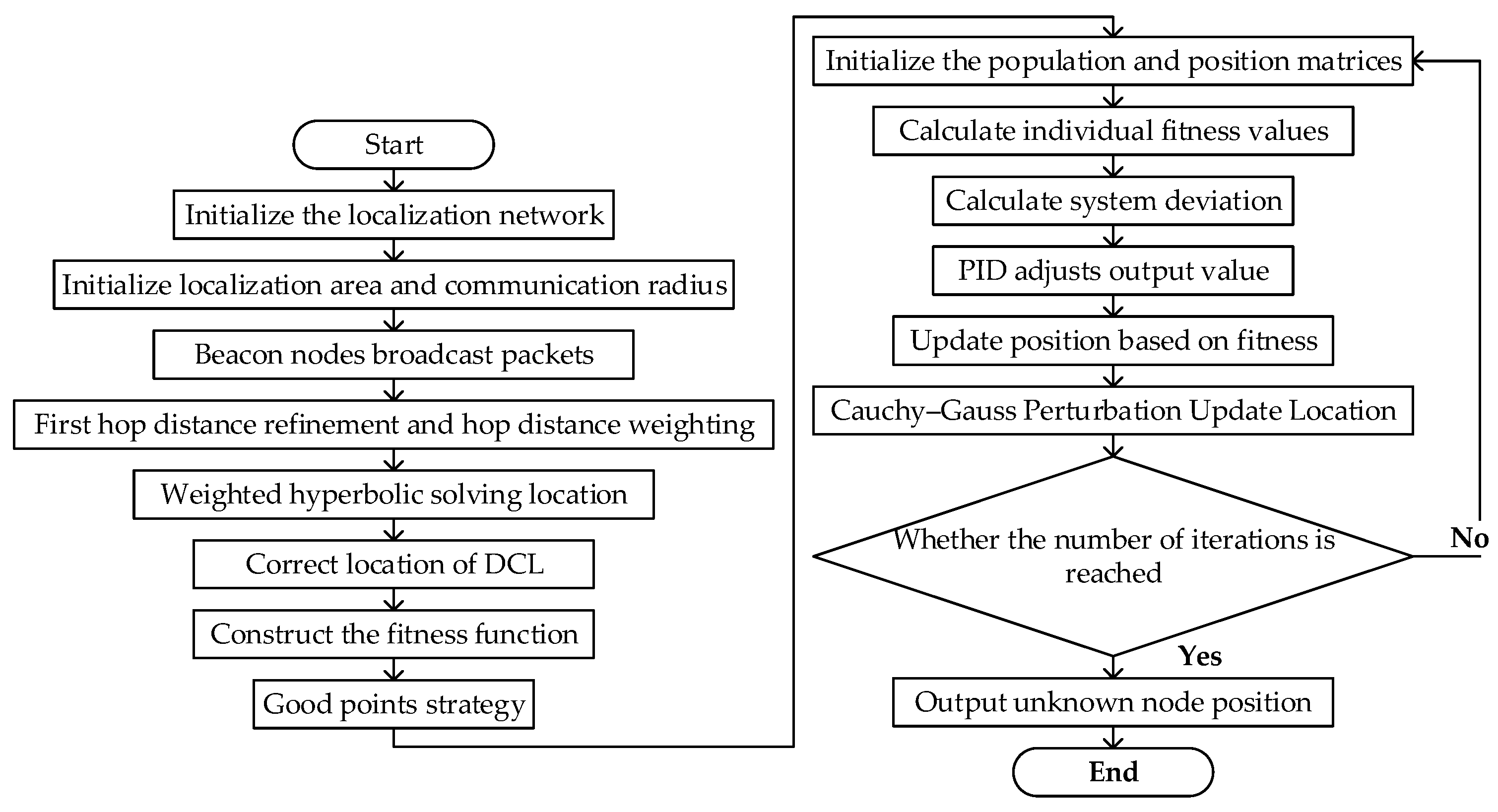
3.2. Two-DimensionalAlgorithm Process

The steps of the IPSA-DV-Hop localization algorithm in the 2D scenario are stated below:

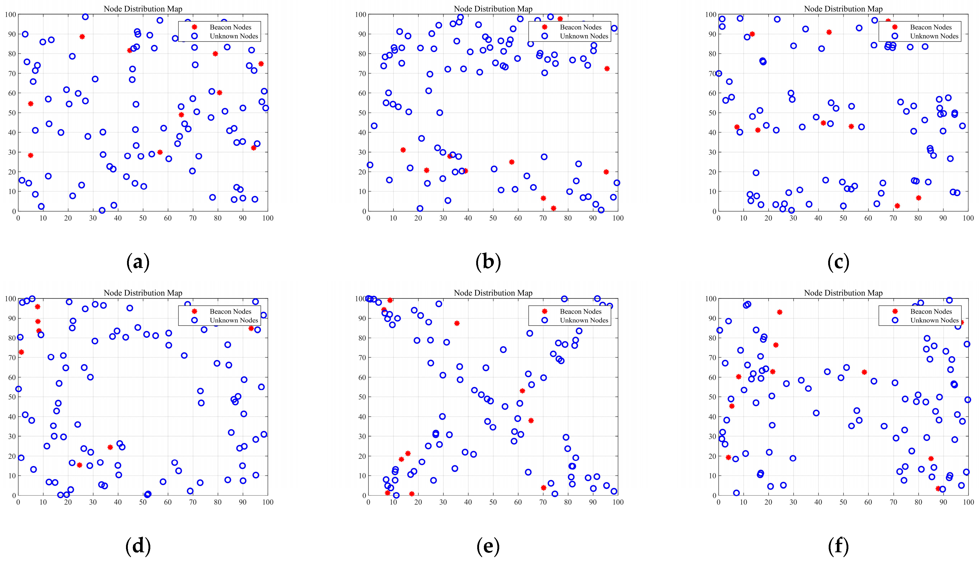
• The initial localization scenario is a square area of $L\times L$ meters with $M$ nodes and $N$ beacon nodes.
• The beacon node broadcasts its location information; the unknown node receives the broadcast packet to obtain the RSSI value and hop distance information between nodes. The unknown node then forwards the hop distance after incrementing it by one, then compares and saves the minimum hop count information to the beacon node.
• The first hop distance is refined using the received RSSI value and the hop count between nodes is calculated based on the refined first hop distance.
• The unknown node calculates its estimated coordinates using the average hop distance and obtains the average hop distance weighted by the distance error.
• The node coordinates are determined using a weighted hyperbolic algorithm, which is combined with the DCL of the node group to further refine the position coordinates.
• The PSA decision variables, constraints, and objective function are initialized. The initial group position coordinates are constructed using the Good Point Set strategy and the fitness function for estimating the unknown node position.
• The system deviation is calculated and iteratively updated using the PID regulation process. The Cauchy–Gaussian perturbation strategy is incorporated in the later stages of the algorithm to output the optimal node position coordinates.

The overall flowchart of the 2D algorithm is shown in Figure 2.

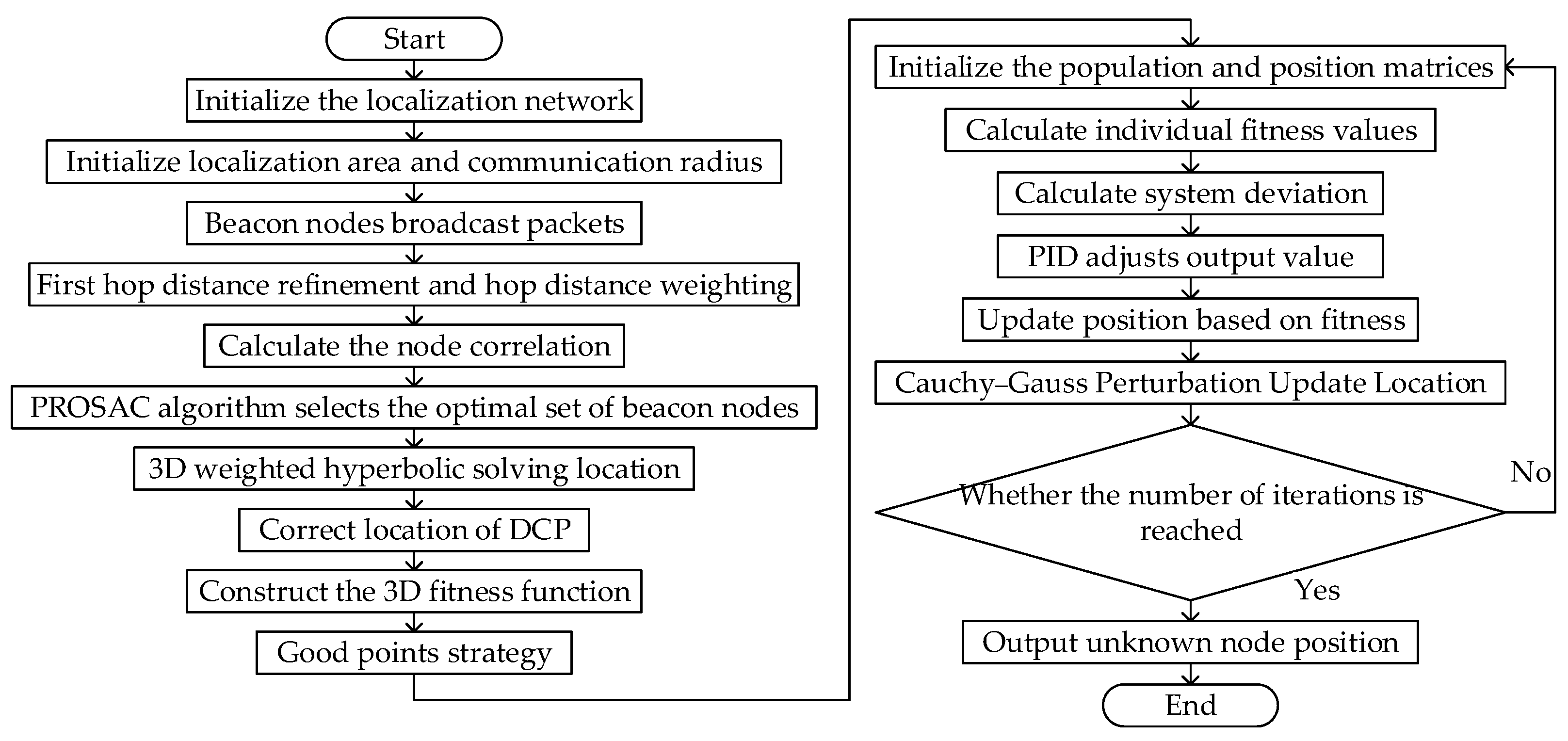
3.3. Three-Dimensional PSA-DV-Hop Algorithm Based on Optimal Subset of Nodes

In practical applications, WSNs inevitably encounter localization challenges in 3D scenarios, such as when the nodes are deployed in rugged terrain. Therefore, the algorithm proposed in this paper is extended to a 3D scenario and improved accordingly.

3.3.1. Node Correlation Degree

To address the aforementioned issues, a subset strategy based on correlation degree is proposed. The correlation degree of beacon nodes integrates multiple similarity metrics to assess the influence and importance of each beacon node. For a beacon node, its distance similarity is defined as the reciprocal of the difference in the number of hops to the unknown node:

$$D{S}_{xy}={\displaystyle \frac{1}{hop{s}_x-hop{s}_y}}$$

(32)

Local path index (LPI) [21] quantifies the similarity of topological relationships between nodes and is expressed as Equation (33):

$$LP{I}_{xy}=A^2+\lambda A^3+\cdots +{\lambda }^{n-2}{A}^n$$

(33)

where $A^n$ represents the set of distinct connectivity paths of length $n$ between beacon node $x$ and y. $\lambda$ is a damping factor that controls the path weights. In this paper, $\lambda$ is set to 0.5, meaning the weight of each order path is half that of the previous order path. This setting balances the contributions of different orders of paths to the LPI while preventing any single order of paths from excessively influencing the result.

The degree of similarity between neighbor nodes can be determined by resource allocation (RA) [22]. The RA between two nodes is defined as the number of resources received by node $y$ from $x$:

$$R{A}_{xy}=\sum _{u\in N\left(x\right)\cap N\left(y\right)}{\displaystyle \frac{1}{\left|N\left(u\right)\right|}}$$

(34)

The correlation of a beacon node, combining the above multiple parameters and weighted by normalization, can be expressed as follows:

$$S_{xy}=\alpha \cdot {\displaystyle \frac{D{S}_{xy}-D{S}_{min}}{D{S}_{max}-D{S}_{min}}}+\beta \cdot {\displaystyle \frac{LP{I}_{xy}-LP{I}_{min}}{LP{I}_{max}-LP{I}_{min}}}+\gamma \cdot {\displaystyle \frac{R{A}_{xy}-R{A}_{min}}{R{A}_{max}-R{A}_{min}}}$$

(35)

where $\alpha$, $\beta$, and $\gamma$ are weighting factors set to 0.5, 0.2, and 0.3, respectively.

3.3.2. The Subset of Optimal Nodes

Random sample consensus (RANSAC) is a parameter estimation algorithm that uses randomly selected initial hypotheses and test sets. However, this approach can result in slow convergence. The PROSAC algorithm improves upon this by ranking all points in the sample set according to rank, assigning higher ranks to the inner points that are more likely to estimate the correct model. By selecting points with higher ranks, PROSAC increases the probability of obtaining the correct model [23]. Incorporating the correlation between beacon nodes into the PROSAC algorithm helps address noise and anomalies in the beacon nodes, thereby improving the robustness of the average distance calculation. The specific implementation steps in the second phase of the DV-Hop algorithm are as follows:

• Beacon node sorting: All beacon nodes are sorted based on their relevance, which is determined by their correlation to the target node.
• Progressive sampling: Sampling begins from the highest-ranked nodes based on the sorting results, and the sampling set is gradually expanded as the number of iterations increases.
• Model evaluation and selection: The Euclidean distance between the selected beacon nodes is calculated and divided by the hop count to obtain the average distance per hop. The quality of the selected beacon node combination is then evaluated by assessing the stability and consistency of the computed average distance per hop.
• Termination condition: The current optimal combination of beacon nodes is selected if it meets the predetermined accuracy requirement.

By utilizing the PROSAC algorithm-based correlation node subset strategy, highly correlated beacon nodes are selected for inclusion in the average hop distance calculation, thereby reducing the influence of nodes with significant errors.

3.3.3. The 3D Weighted Hyperbolic Algorithm

Extending the hyperbolic localization algorithm to 3D introduces challenges in estimating unknown node positions, especially when four nodes are nearly coplanar. To address this, the position of the localization unit is corrected using the degree of coplanarity (DCP) [24]. The ratio of the tetrahedral radius can be expressed as follows:

$$\rho ={\displaystyle \frac{216v^2}{{\sum }_{i=0}^3{s}_i\cdot \sqrt{\left(a+b+c\right)\left(a+b-c\right)\left(a-b+c\right)\left(b+c-a\right)}}}$$

(36)

where $\rho$ ranges from 0 to 1; as it approaches 0, these four points become increasingly coplanar.

An effective threshold is set based on the DCP, and nodes that exceed this threshold are excluded from the localization process. The 3D weighted hyperbolic algorithm is then applied to the selected set of nodes. The fitness function of the PSA for the 3D scenario is expressed by Equation (37):

$$fitness(x, y, z)={\sum }_{i=1}^M{\left[\sqrt{{\left(x_i-x_u\right)}^2+{\left(y_i-y_u\right)}^2+{\left(z_i-z_u\right)}^2}-d_{iu}\right]}^2$$

(37)

Due to the increased complexity of solving in a 3D scenario, both the number of iterations and population size must be increased accordingly. The coordinates are then optimized using DCP weights. The 3D IPSA-DV-Hop algorithm is employed to calculate the position coordinates, achieving a notable improvement in localization accuracy with only a slight increase in computational complexity.

The overall flowchart of the 3D algorithm is presented in Figure 3:

3.4. Analysis of Algorithm Complexity

In WSNs, node applications are typically constrained by energy and computational resources. Since different algorithms require varying amounts of time to optimize the same problem, analyzing the computational complexity of any proposed algorithm becomes essential.

We use big $O$ notation to analyze time complexity. Let $M$ represent the number of nodes and $N$ represent the number of beacon nodes. The population size in the PSA is denoted by $n$, and the maximum number of iterations is $T$. The dimension of the algorithm is represented by $D$. The time complexity for population initialization and position updating in the PSA can be expressed as $O(n)$ and $O(nTD)$, respectively. The complexity of the weighted hyperbolic process is $O(M^2-MN)$. In a 3D scenario, the PROSAC strategy is applied with a complexity of $O(N^2)$. Considering the proportion of beacon nodes is relatively small, the overall time complexity of the proposed algorithm can be approximated as $O(M^2+nTD)$ and $O(M^3+nTD+N^2)$ in 2D and 3D scenarios, respectively. In contrast, DV-Hop uses the least square method to localize sensor nodes, with computational complexities of $O(M^2)$ and $O(M^3)$ in 2D and 3D scenarios, respectively. The proposed algorithm has moderately improved the localization accuracy by slightly increasing the computational complexity. This increase is deemed acceptable for the benefits it offers.

4. Simulation Results and Analysis

To validate the performance of the algorithm proposed in this paper, we conducted simulation experiments in various scenarios on the MATLAB 2023b platform.

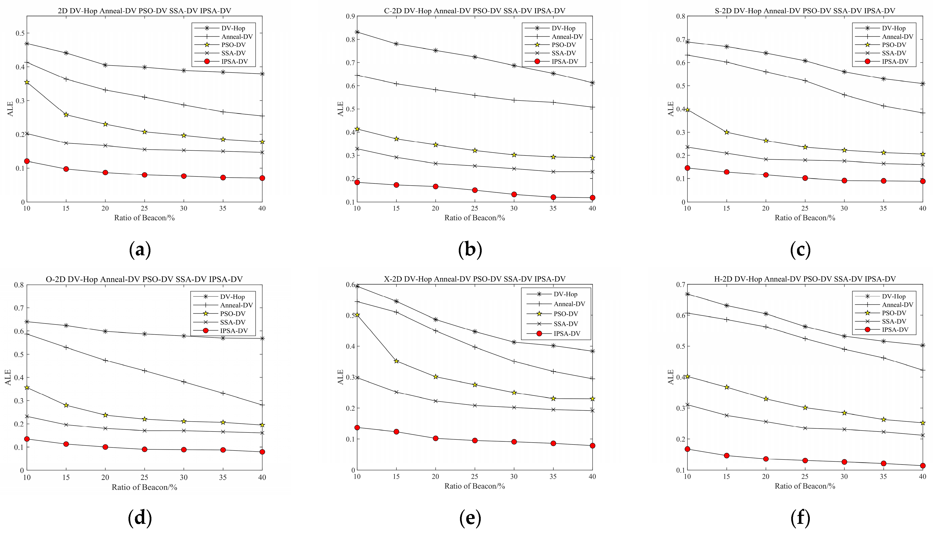
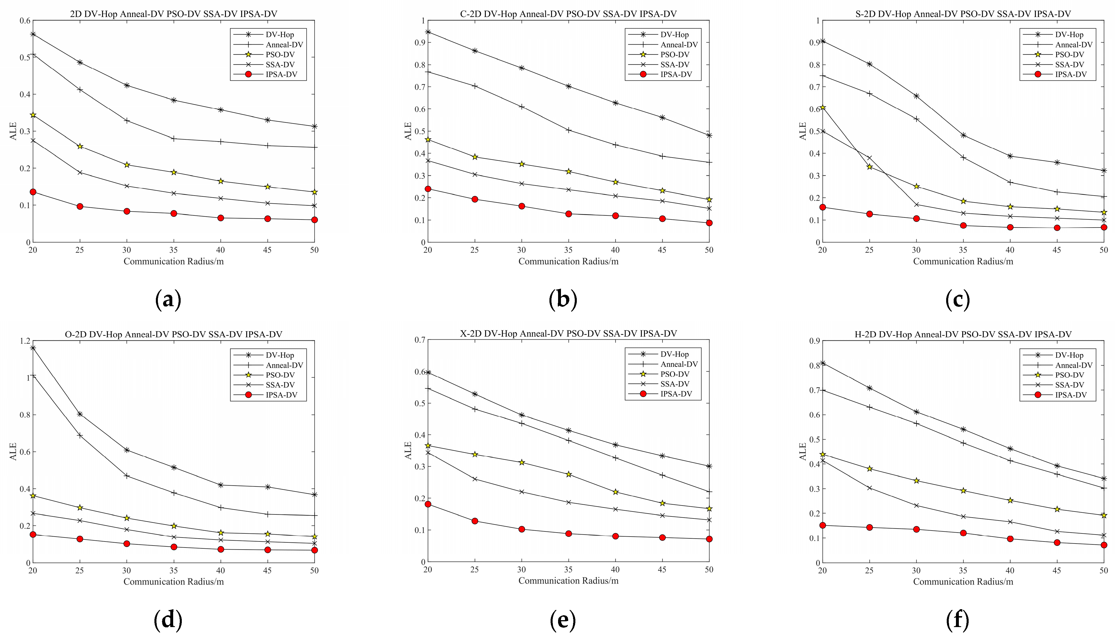
4.1. Two-DimensionalSimulation Parameters and Results

The proposed algorithm was compared with classical DV-Hop, DV-Hop based on simulated annealing, DV-Hop based on particle swarm optimization (PSO), and DV-Hop based on the sparrow search algorithm (SSA). In the simulations, the default parameters were set as follows: 100 nodes, 20% beacon nodes, and a communication radius of 30 m. A total of 100 simulations were conducted, and the average value was calculated to minimize random errors. The normalized average localization error (ALE) is given by Equation (38):

$$ALE={\displaystyle \frac{{\sum }_{i=1}^N\sqrt{{\left(x_{iest}-x_i\right)}^2+{\left(y_{iest}-y_i\right)}^2}}{N\cdot R}}$$

(38)

where $\left(x_{iest}, y_{iest}\right)$ represents the estimated location of the unknown nodes, and $\left(x_i, y_i\right)$ represents the true location of unknown nodes. The simulation parameters were set as shown in

Table 1. Two-dimensional simulation parameters.

Simulation Parameters	Value
Scenario size	100 m × 100 m
Communication radius	20–50 m
Ratio of beacon	10–40%
Number of nodes	50–150
DOI	0–0.1

.

The simulation scenarios, respectively, used a 2D rectangular area of 100 m × 100 m and anisotropic network areas with X-shape, H-shape, S-shape, C-shape, and O-shape topologies. The node topology distributions of the 2D scenarios are shown in Figure 4.

The proportion of beacon nodes increased from 10% to 40%, and the simulation results of each algorithm are shown in Figure 5. The proposed algorithm outperformed the others across all scenarios with varying beacon node ratios, demonstrating better performance in scenarios with a higher proportion of beacon nodes. This improvement is attributed to the more-connected topology, which enables greater node coverage and more detailed network information.

The total number of nodes increased from 50 to 150, and the simulation results of each algorithm are shown in Figure 6. As the number of nodes increased, the proposed algorithm demonstrated robustness, remaining less affected by network topology and maintaining high accuracy even with complex node distributions.

The communication radius increased from 20 m to 50 m, and the comparative results of the algorithms under different topological distributions are shown in Figure 7. The proposed algorithm continues to exhibiting higher accuracy in small-scale anisotropic networks, demonstrating its high stability and resilience to changes in network size.

The computational complexity of the proposed algorithm has been analyzed and compared, with the specific runtime of different algorithms in the 2D scenarios presented in

Table 2. The computational complexity comparison in 2D scenarios.

Algorithms	Rectangular Area	C-Shaped Area	S-Shaped Area	O-Shaped Area	X-Shaped Area	H-Shaped Area
DV-Hop	1.1	1.6	1.7	1.7	1.4	1.4
Anneal-DV	15.2	16.2	18.2	18.5	15.6	16.3
PSO-DV	11.1	12.9	13.5	14.6	13.2	13.4
SSA-DV	15.1	16.5	16.7	21.8	18.1	17.6
IPSA-DV	19.7	21.4	22.2	25.6	21.2	23.5

. Compared to other algorithms, the proposed algorithm exhibits a slight increase in complexity. However, since the algorithm mainly operates on the beacon nodes, which are typically equipped with sufficient energy, its impact on the overall network remains minimal.

The localization errors for DOI values of 0, 0.05, and 0.1 were compared as shown in Figure 8. In Figure 8a, the proportion of beacon nodes increases from 10% to 40%, and in Figure 8b, the communication radius increases from 20 m to 50 m. The impact on the classical DV-Hop algorithm was more significant, with the localization error increasing by approximately 10%. In contrast, the proposed algorithm was less affected, with the localization error increasing by only about 2%. These results collectively demonstrated that the proposed algorithm exhibited stronger robustness.

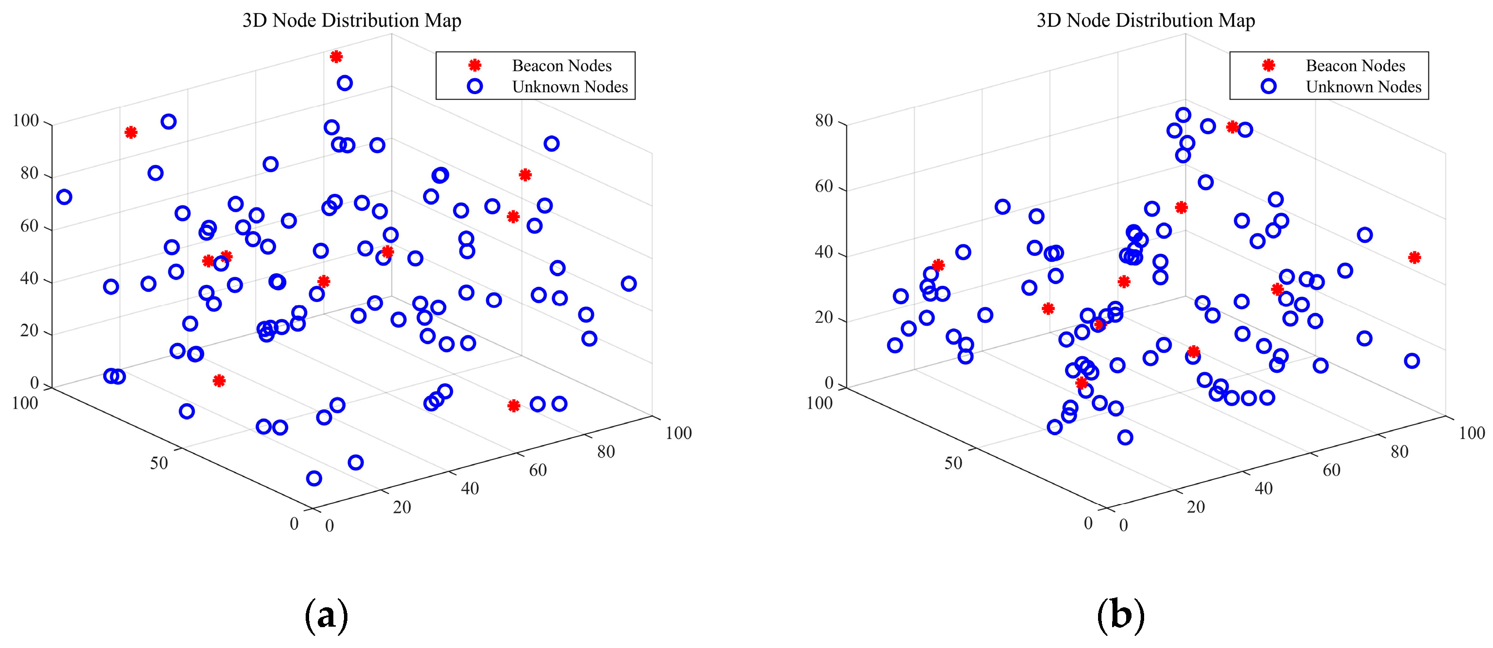
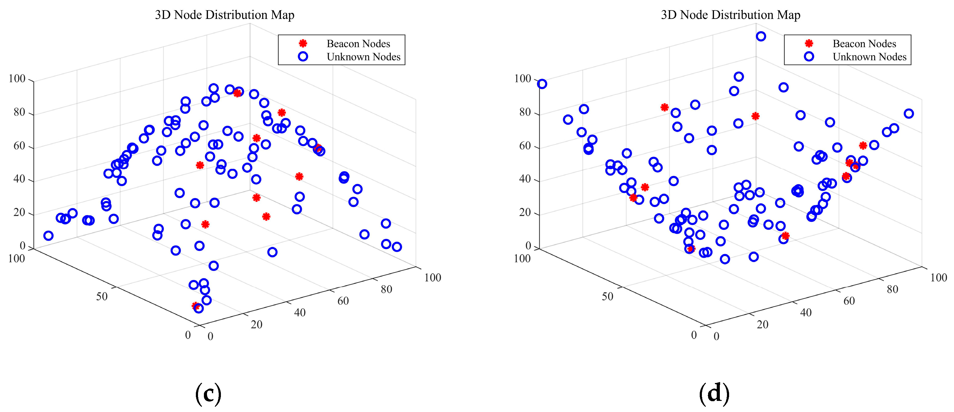
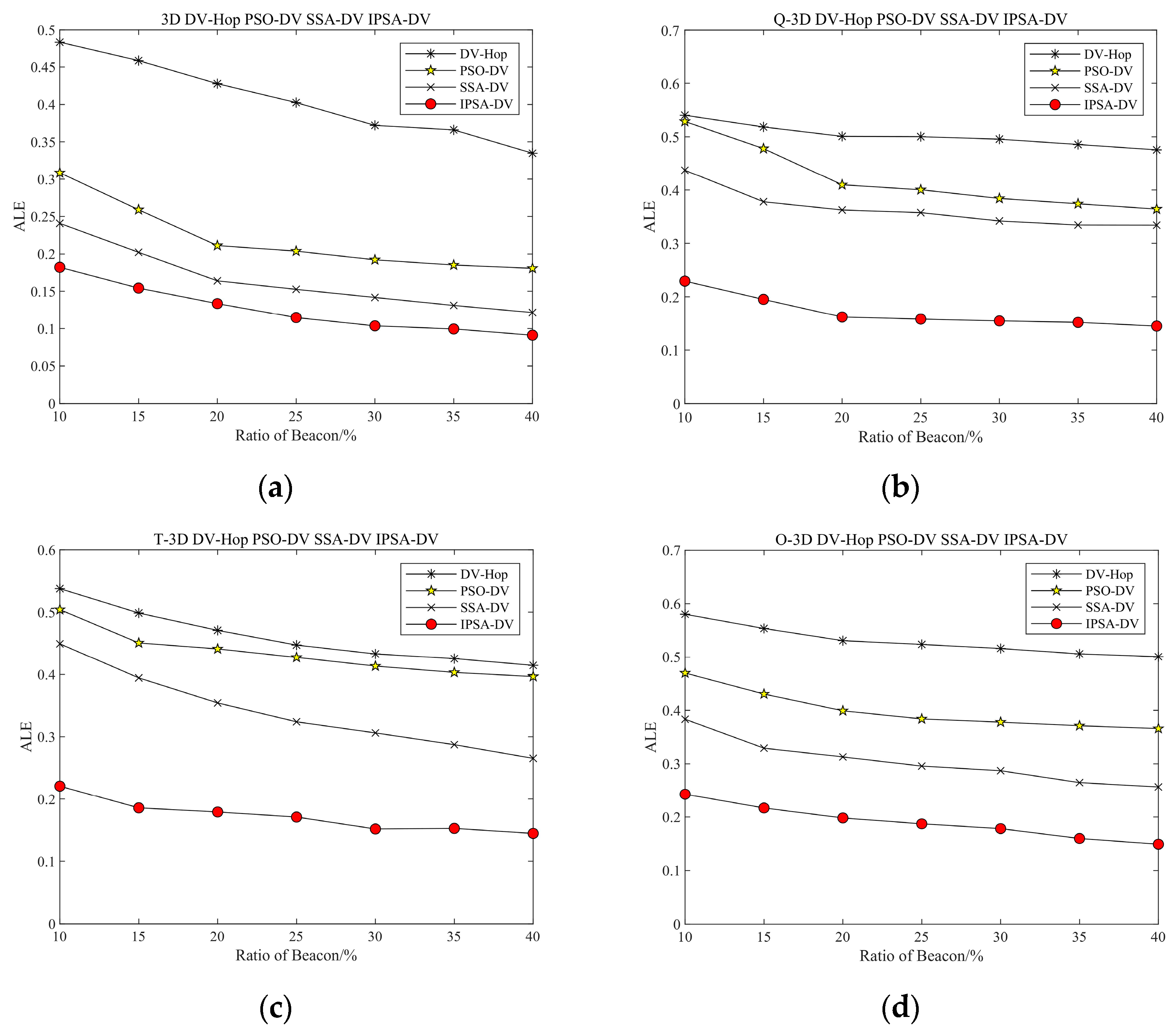
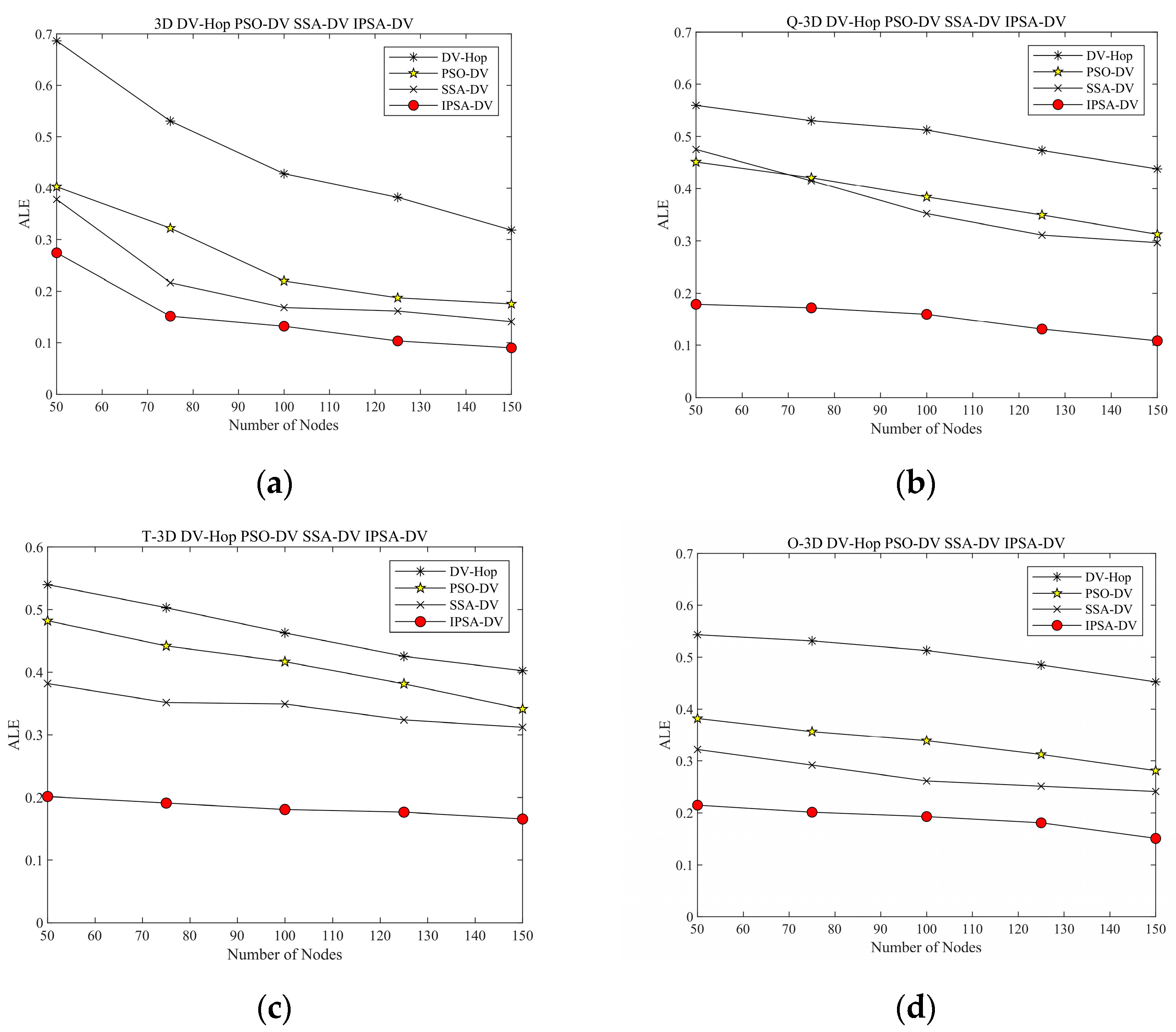
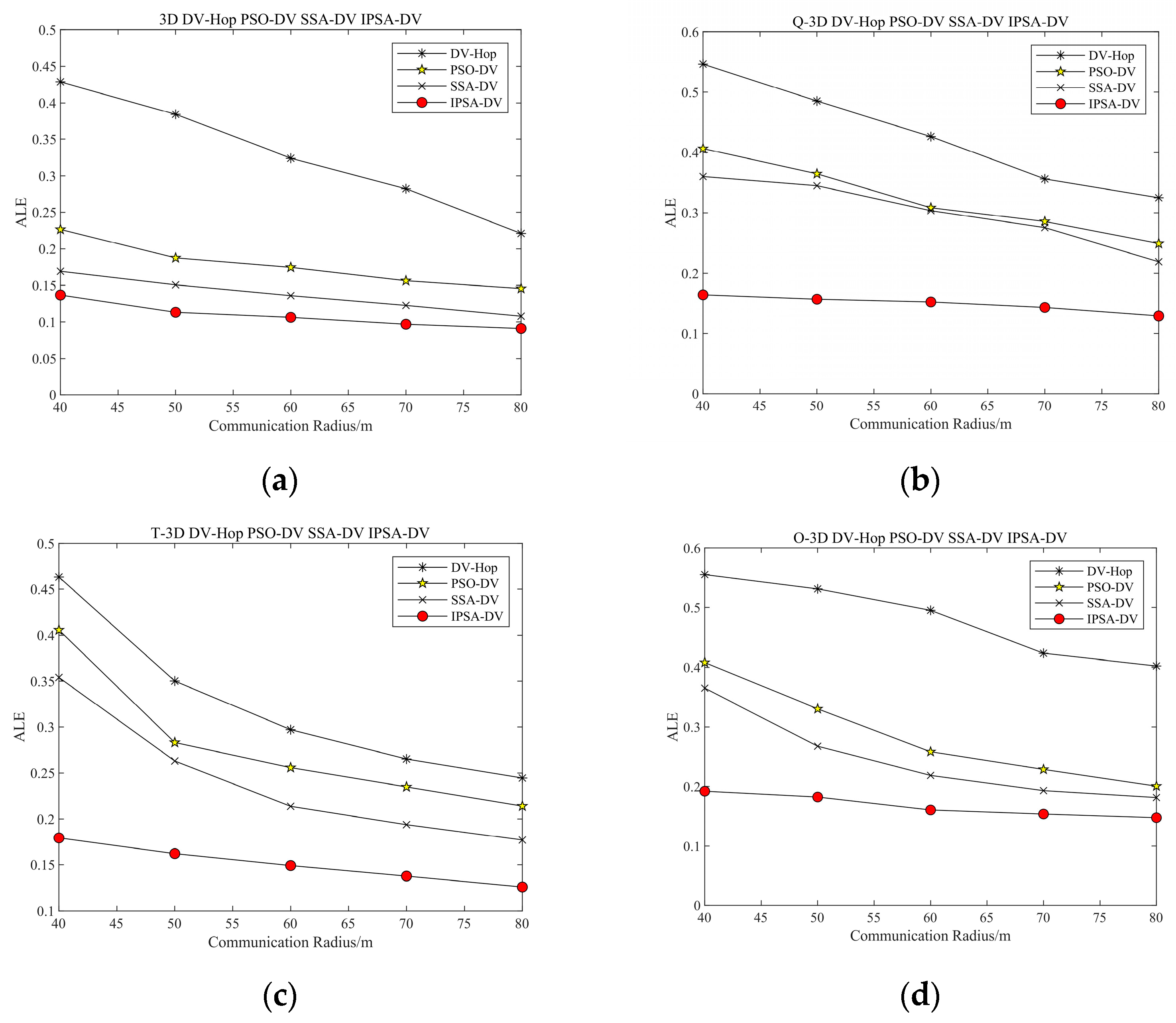
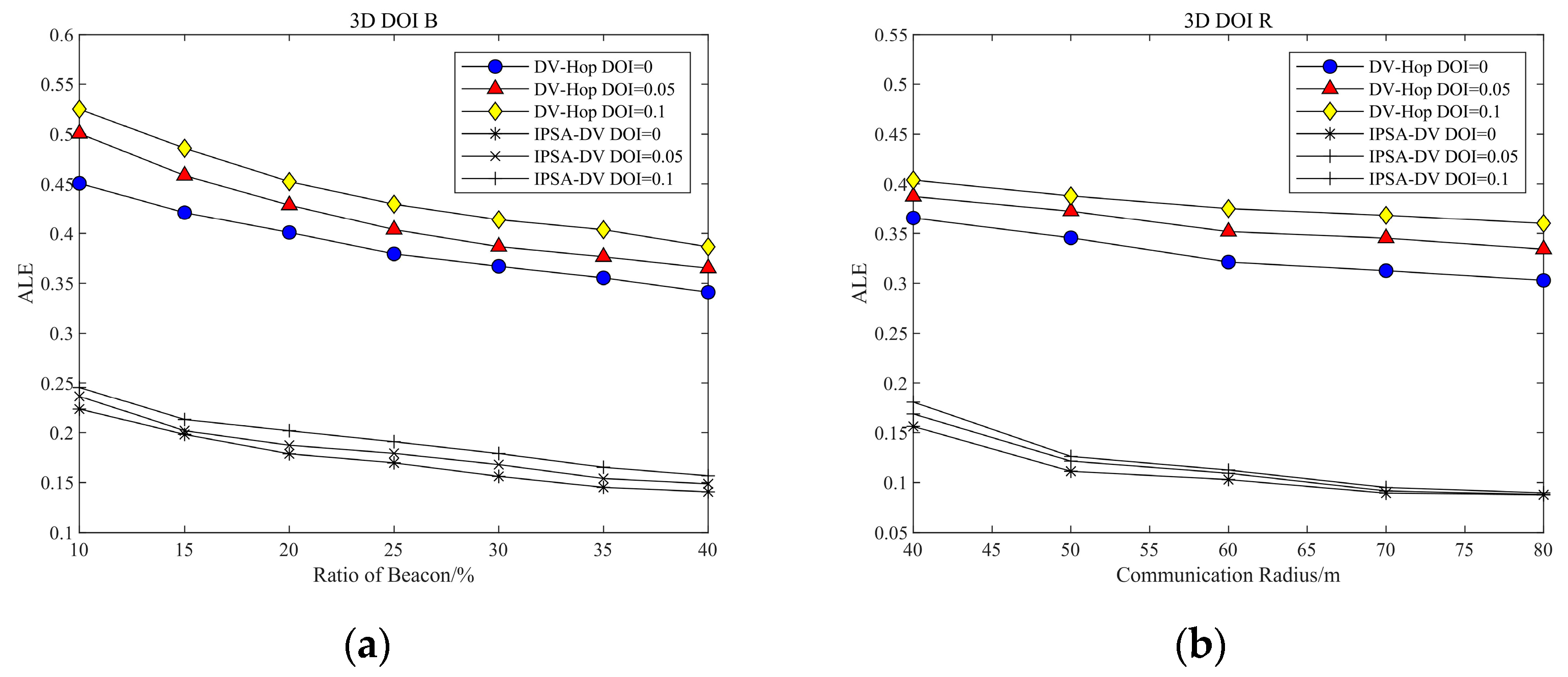
4.2. Three-Dimensional Simulation Parameters and Results

The proposed algorithm was compared with 3D DV-Hop, 3D DV-Hop based on PSO, and 3D DV-Hop based on SSA. The default parameters for the simulations were set to 100 nodes, 20% beacon nodes, and a communication radius of 40 m. The normalized ALE in the 3D scenarios can be expressed by Equation (39)

$$AL{E}_{3\mathrm{D}}={\displaystyle \frac{{\sum }_{i=1}^N\sqrt{{\left(x_{iest}-x_i\right)}^2+{\left(y_{iest}-y_i\right)}^2+{\left(z_{iest}-z_i\right)}^2}}{N\cdot R}}$$

(39)

where $\left(x_{iest}, y_{iest}, z_{iest}\right)$ represents the estimated coordinates of the unknown nodes. $\left(x_i, y_i, z_i\right)$ represents the true location of unknown nodes. The simulation parameters in 3D scenarios were set as shown in

Table 3. Three-Dimensional simulation parameters.

Simulation Parameters	Value
Scenario size	100 m × 100 m × 100 m
Communication radius	40–80 m
Ratio of beacon	10–40%
Number of nodes	50–150
DOI	0–0.1

.

The simulation scenarios included a 100 m × 100 m × 100 m 3D cubic terrain and a 3D anisotropic network distribution area consisting of rugged, hilly, and valley terrains. Figure 9 illustrates the node topology distributions in the 3D scenarios.

The proportion of beacon nodes increased from 10% to 40%, and the simulation results of each algorithm are shown in Figure 10. The proposed algorithm outperformed the others across various beacon node ratios, with the localization error gradually decreasing as the number of beacons increased.

The total number of nodes increased from 50 to 150, and the simulation results of each algorithm are shown in Figure 11. The communication radius increased from 40 m to 80 m, and the comparative effects of each algorithm under various topological distributions are shown in Figure 12.

As the network size increases, the localization error of the proposed algorithm initially decreases and then levels off. This algorithm consistently outperforms the others in all scenarios, demonstrating stable localization accuracy that is less affected by network size. As the communication radius increases, the localization accuracy of all algorithms improves to varying extents. However, the proposed algorithm continues to maintain high localization accuracy even with a large communication radius.

The computational complexity of the proposed algorithm in 3D scenarios was analyzed and compared. The default parameter values were used in the simulation tests, with the specific results presented in

Table 4. The computational complexity comparison in 3D scenarios.

Algorithms	Cubic Terrain	Rugged Terrain	Hilly Terrain	Valley Terrain
3D DV-Hop	3.6	5.2	6.3	6.9
3D PSO-DV	18.5	19.9	21.2	21.4
3D SSA-DV	28.9	28.5	29.6	30.2
3D PSA-DV	32.8	31.5	33.2	38.3

.

Figure 13 shows the comparison of the localization error at DOI values of 0, 0.05, and 0.1. Figure 13a shows the effect of increasing the proportion of beacon nodes from 10% to 40%, while Figure 13b demonstrates the impact of increasing the communication radius from 40 m to 80 m.

The results indicated that localization errors increase with the DOI for all algorithms. However, the classical DV-Hop algorithm is more significantly affected. The proposed algorithm, by using the optimal node subset strategy, ensures the reliability of the selected beacon nodes, thereby reducing the sensitivity of localization errors to irregular communication. This highlights the superior robustness and reliability of the proposed algorithm for practical applications.

5. Conclusions

This paper proposed an enhancement to the DV-Hop localization algorithm by the introduction of the IPSA-DV-Hop algorithm, which incorporates weighted hyperbolic refinement. In the first step, the hop distance was refined by correcting the RSSI. During the hop distance calculation phase, a weighted hyperbolic algorithm based on DCL replaced the original least squares method. The optimized PSA further reduced the localization error. When extended to 3D scenarios, the optimal node subset strategy, based on the PROSAC algorithm, effectively reduced beacon node hop distance errors. Position calculation was performed using the 3D hyperbolic algorithm, which was augmented with DCP for improved accuracy. Simulation experiments were conducted in 2D using random, C-shaped, H-shaped, S-shaped, and X-shaped anisotropic network distributions. In 3D, simulations were performed with random, hilly, valley, and rugged terrains. By comparing localization accuracy across various complex network environments, the proposed algorithm demonstrated superior accuracy in both isotropic and anisotropic networks. Despite a slight increase in computational complexity, it was demonstrated to be robust, exhibiting low sensitivity to network topology and maintaining strong stability under irregular radio communication conditions.

References

1. Patel, N.R.; Kumar, S. Wireless Sensor Networks’ Challenges and Future Prospects. In Proceedings of the 2018 International Conference on System Modeling & Advancement in Research Trends (SMART), Moradabad, India, 23–24 November 2018; pp. 60–65. [Google Scholar]
2. Sivasakthiselvan, S.; Nagarajan, V. Localization Techniques of Wireless Sensor Networks: A Review. In Proceedings of the 2020 International Conference on Communication and Signal Processing (ICCSP), Chennai, India, 28–30 July 2020; pp. 1643–1648. [Google Scholar]
3. Park, K.-D.; Yoon, W.-J.; Lee, J.-S. Reduction of Multipath Effect in GNSS Positioning by Applying Pseudorange Acceleration as Weight. Sensors 2024, 24, 6880. [Google Scholar] [CrossRef] [PubMed]
4. Saad, E.; Elhosseini, M.; Haikal, A.Y. Recent Achievements in Sensor Localization Algorithms. Alex. Eng. J. 2018, 57, 4219–4228. [Google Scholar] [CrossRef]
5. Chadha, J.; Jain, A. Anatomization on Range-Free Localization Algorithms in Wireless Sensor Networks. In Proceedings of the 2019 2nd International Conference on Power Energy, Environment and Intelligent Control (PEEIC), Greater Noida, India, 18–19 October 2019; pp. 489–492. [Google Scholar]
6. Cao, Y.; Qian, Y.; Wang, Z. DV-Hop Based Localization Algorithm Using Node Negotiation and Multiple Communication Radii for Wireless Sensor Network. Wirel. Netw. 2023, 29, 3493–3513. [Google Scholar] [CrossRef]
7. Achroufene, A. RSSI-Based Geometric Localization in Wireless Sensor Networks. J. Supercomput. 2023, 79, 5615–5642. [Google Scholar] [CrossRef]
8. Singh, P.; Mittal, N.; Singh, P. A Novel Hybrid Range-Free Approach to Locate Sensor Nodes in 3D WSN Using GWO-FA Algorithm. Telecommun. Syst. 2022, 80, 303–323. [Google Scholar] [CrossRef]
9. Mohanta, T.K.; Das, D.K. A Three-Dimensional Wireless Sensor Network with an Improved Localization Algorithm Based on Orthogonal Learning Class Topper Optimization. Ann. Telecommun. 2023, 78, 475–489. [Google Scholar] [CrossRef]
10. Niculescu, D. DV Based Positioning in Ad Hoc Networks. Telecommun. Syst. 2003, 22, 267–280. [Google Scholar] [CrossRef]
11. Cai, X.; Hu, K.; Zhang, F.; Li, W.; Li, Y.; Zhang, Z. Research on Node Location Technology Based on Improved Particle Swarm Optimization. In Proceedings of the 2019 IEEE Symposium Series on Computational Intelligence (SSCI), Xiamen, China, 6–9 December 2019; pp. 2833–2837. [Google Scholar]
12. Xue, D. Research of Localization Algorithm for Wireless Sensor Network Based on DV-Hop. EURASIP J. Wirel. Commun. Netw. 2019, 2019, 218. [Google Scholar] [CrossRef]
13. Sharma, N.; Gupta, V. Meta-Heuristic Based Optimization of WSNs Localisation Problem—A Survey. Procedia Comput. Sci. 2020, 173, 36–45. [Google Scholar] [CrossRef]
14. Srivastava, A.; Mishra, P.K. A Survey on WSN Issues with Its Heuristics and Meta-Heuristics Solutions. Wirel. Pers. Commun. 2021, 121, 745–814. [Google Scholar] [CrossRef]
15. Gao, Y. PID-Based Search Algorithm: A Novel Metaheuristic Algorithm Based on PID Algorithm. Expert Syst. Appl. 2023, 232, 120886. [Google Scholar] [CrossRef]
16. Niu, S.S.; Xiao, D. Basic PID Control. In Process Control; Advances in Industrial Control; Springer International Publishing: Cham, Switzerland, 2022; pp. 67–114. [Google Scholar]
17. Bhat, S.J.; Santhosh, K.V. Localization of Isotropic and Anisotropic Wireless Sensor Networks in 2D and 3D Fields. Telecommun. Syst. 2022, 79, 309–321. [Google Scholar] [CrossRef]
18. He, T.; Huang, C.; Blum, B.M.; Stankovic, J.A.; Abdelzaher, T. Range-Free Localization Schemes for Large Scale Sensor Networks. In Proceedings of the 9th Annual International Conference on Mobile Computing and Networking, San Diego, CA, USA, 14–19 September 2003; pp. 81–95. [Google Scholar]
19. Poggi, C.; Mazzini, G. Collinearity for Sensor Network Localization. In Proceedings of the 2003 IEEE 58th Vehicular Technology Conference. VTC 2003-Fall (IEEE Cat. No.03CH37484), Orlando, FL, USA, 6–9 October 2003; pp. 3040–3044. [Google Scholar]
20. Elsawah, A.M.; Fang, K.-T.; Deng, Y.H. Some Interesting Behaviors of Good Lattice Point Sets. Commun. Stat. Simul. Comput. 2021, 50, 3650–3668. [Google Scholar] [CrossRef]
21. Kumar, A.; Singh, S.S.; Singh, K.; Bisis, B. Link Prediction Techniques, Applications, and Performance: A Survey. Phys. Stat. Mech. Its Appl. 2020, 553, 124289. [Google Scholar] [CrossRef]
22. Lü, L.; Zhou, T. Link Prediction in Complex Networks: A Survey. Phys. Stat. Mech. Its Appl. 2011, 390, 1150–1170. [Google Scholar] [CrossRef]
23. Chum, O.; Matas, J. Matching with PROSAC—Progressive Sample Consensus. In Proceedings of the 2005 IEEE Computer Society Conference on Computer Vision and Pattern Recognition (CVPR’05), San Diego, CA, USA, 20–25 June 2005; Volume 1, pp. 220–226. [Google Scholar]
24. Reddy, M.R.; Chandra, M.L.R. An Improved 3D-DV-Hop Localization Algorithm to Improve Accuracy for 3D Wireless Sensor Networks. SN Comput. Sci. 2024, 5, 245. [Google Scholar] [CrossRef]
Figure 1. Radiation at different DOIs. (a) DOI = 0; (b) DOI = 0.05; (c) DOI = 0.1.
Mathematics 12 03908 g001
Figure 2. Flowchart of the 2D algorithm.
Mathematics 12 03908 g002
Figure 3. Flowchart of the 3D algorithm.
Mathematics 12 03908 g003
Figure 4. Node distribution maps in 2D scenarios. (a) Rectangular area. (b) C-shaped area. (c) S-shaped area. (d) O-shaped area. (e) X-shaped area. (f) H-shaped area.
Mathematics 12 03908 g004
Figure 5. Comparison of localization error under different beacon ratios in 2D scenarios. (a) Rectangular area. (b) C-shaped area. (c) S-shaped area. (d) O-shaped area. (e) X-shaped area. (f) H-shaped area.
Mathematics 12 03908 g005
Figure 6. Comparison of localization error under different numbers of nodes in 2D scenarios. (a) Rectangular area. (b) C-shaped area. (c) S-shaped area. (d) O-shaped area. (e) X-shaped area. (f) H-shaped area.
Mathematics 12 03908 g006
Figure 7. Comparison of localization error under different communication radii in 2D scenarios. (a) Rectangular area. (b) C-shaped area. (c) S-shaped area. (d) O-shaped area. (e) X-shaped area. (f) H-shaped area.
Mathematics 12 03908 g007
Figure 8. Comparison of localization error under different DOIs in 2D scenarios. (a) Two-dimensional variable ratio of beacon. (b) Two-dimensional variable communication radius.
Mathematics 12 03908 g008
Figure 9. Node distribution maps in 3D scenarios. (a) Cubic terrain. (b) Rugged terrain. (c) Hilly terrain. (d) Valley terrain.
Mathematics 12 03908 g009aMathematics 12 03908 g009b
Figure 10. Comparison of localization errors under different beacon ratios in 3D scenarios. (a) Cubic terrain. (b) Rugged terrain. (c) Hilly terrain. (d) Valley terrain.
Mathematics 12 03908 g010
Figure 11. Comparison of localization errors under different numbers of nodes in 3D scenarios. (a) Cubic terrain. (b) Rugged terrain. (c) Hilly terrain. (d) Valley terrain.
Mathematics 12 03908 g011
Figure 12. Comparison of localization errors under different communication radii in 3D scenarios. (a) Cubic terrain. (b) Rugged terrain. (c) Hilly terrain. (d) Valley terrain.
Mathematics 12 03908 g012
Figure 13. Comparison of localization errors under different communication radii in 3D scenarios. (a) Three-dimensional variable beacon ratio. (b) Three-dimensional variable communication radius.
Mathematics 12 03908 g013