Semi-Implicit Numerical Integration of Boundary Value Problems

Abstract

The numerical solution to boundary differential problems is a crucial task in modern applied mathematics. Usually, implicit integration methods are applied to solve this class of problems due to their high numerical stability and convergence. The known shortcoming of implicit algorithms is high computational costs, which can become unacceptable in the case of numerous right-hand side function calls, which are typical when solving boundary problems via the shooting method. Meanwhile, recently semi-implicit numerical integrators have gained major interest from scholars, providing an efficient trade-off between computational costs, stability, and precision. However, the application of semi-implicit methods to solving boundary problems has not been investigated in detail. In this paper, we aim to fill this gap by constructing a semi-implicit boundary problem solver and comparing the performance of explicit, semi-implicit, semi-explicit, and implicit methods using a set of linear and nonlinear test boundary problems. The novel blinking solver concept is introduced to overcome the main shortcoming of the semi-implicit schemes, namely, the low convergence on exponential solutions. The numerical stability of the blinking semi-implicit solver is investigated and compared with existing methods by plotting the stability regions. The performance plots for investigated methods are obtained as a dependence between global truncation error and estimated computation time. The experimental results confirm the assumption that semi-implicit numerical methods can significantly outperform both explicit and implicit solvers while solving boundary problems, especially in the proposed blinking modification. The results of this study can be efficiently used to create software for solving boundary problems, including partial derivative equations. Constructing semi-implicit numerical methods of higher-accuracy orders is also of interest for further research.

1. Introduction

Mathematical models representing various physical processes are key objects of research in mathematical physics. The theory of elasticity; wave functions in electrodynamics; acoustic models; hydrodynamic models; chaos theory; etc.—all these phenomena are usually described by differential or differential-algebraic equations, often involving partial derivatives [1]. The general problem statement assumes creating a mathematical model that describes certain physical, technical, or social processes with the necessary degree of accuracy and adequacy. One crucial problem of differential calculus that falls into this category is the boundary value problem (BVP) [2,3,4]. The most straightforward approach to solving BVPs is finding a solution for the corresponding differential equation while ensuring that boundary conditions in both initial and final points are satisfied. It is important to ensure that the boundary conditions are set correctly and the solution meets the conditions of existence and uniqueness. At the same time, the solution must continuously depend on the initial values [5,6]. The main general methods for solving this class of differential problems were developed from specific approaches to solving certain physical problems. Advances in this field have led to the development of new methods for solving problems related to the flow of a process [7]. To determine the uniqueness of the solution, the specific boundary conditions are to be set. BVPs can be solved by various numerical methods of approximation. The most common approach is reducing the BVP to a Cauchy problem [8], which can then be solved numerically using ODE solvers. It should be noted that while various modifications of the explicit Runge–Kutta methods are used in common software applications, they are not always the best possible solution in terms of precision and stability. Many sophisticated numerical schemes are integrated into popular mathematical software, such as implicit Runge–Kutta or linear multistep methods. The convergence of finite-difference schemes is of utmost importance in solving BVPs; therefore, implicit methods are favorable. However, this straightforward approach does not completely satisfy the performance requirements due to multiple calls of right-hand function and computationally complex Newton’s method iterations. In recent years, symmetric numerical methods have emerged as an efficient approach to solving Hamiltonian problems. Such methods allow for the preservation of some important properties of simulated systems such as Hamiltonian energy and phase-space volume [9]. Some of the most computationally efficient symmetric integrators are [10] semi-implicit methods, which have recently received great attention from scholars due to simple implementation, low computational costs, and good suitability for solving nonlinear problems. Some promising representatives of this class are semi-explicit and semi-implicit composition schemes [11,12]. Being a reasonable trade-off between explicit and implicit methods, semi-implicit and semi-explicit integrators possess adequate numerical stability and can theoretically greatly increase the overall performance of algorithms for solving boundary problems [11]. However, the performance of semi-implicit methods while solving boundary value problems has not yet been analyzed in detail. In addition, some previous studies claim that semi-implicit integration can demonstrate weak convergence in the case of highly exponential solutions.

In this paper, we investigate the possibility of solving boundary problems using semi-implicit and semi-explicit numerical methods. We consider the known shortcomings of the semi-implicit approach and reveal them using the test BVP with an exponential solution. To overcome these issues, we propose a new so-called “blinking” method, which is more efficient than other considered numerical schemes. The main contributions of our study are as follows:

• Several semi-explicit and semi-implicit numerical integration schemes of order 2 are modified for solving boundary value problems:

  -

  Semi-explicit midpoint method (SEMP) (10);

  -

  Semi-implicit midpoint method (SIMP) (11);

  -

  CD composition method (12) and (13);

• It is discovered that the presence of highly exponential components in the system dynamics results in an unacceptable loss of the convergence for both semi-explicit and semi-implicit methods (Section 3.3.1).
• A new Blinking scheme for the numerical solution to boundary problems is introduced as a combination of semi-explicit and semi-implicit methods for improved convergence.
• A performance comparison of the proposed scheme with known explicit and implicit counterparts is given.
• The computational efficiency of the proposed method is confirmed experimentally by computational experiments with test BVPs (Section 3).

The rest of the paper is organized as follows. In Section 2, we consider the basics of semi-implicit integration and describe the application of semi-implicit and semi-explicit numerical methods to solving boundary problems. The novel “blinking” method is proposed to overcome the convergence issues typical for semi-implicit integration. The stability regions are depicted to evaluate the numerical stability of the investigated methods. In Section 3, the set of test problems is given and the performance of considered methods and algorithms is evaluated using performance plots and truncation error analysis. Finally, Section 4 concludes the paper.

2. Materials and Methods

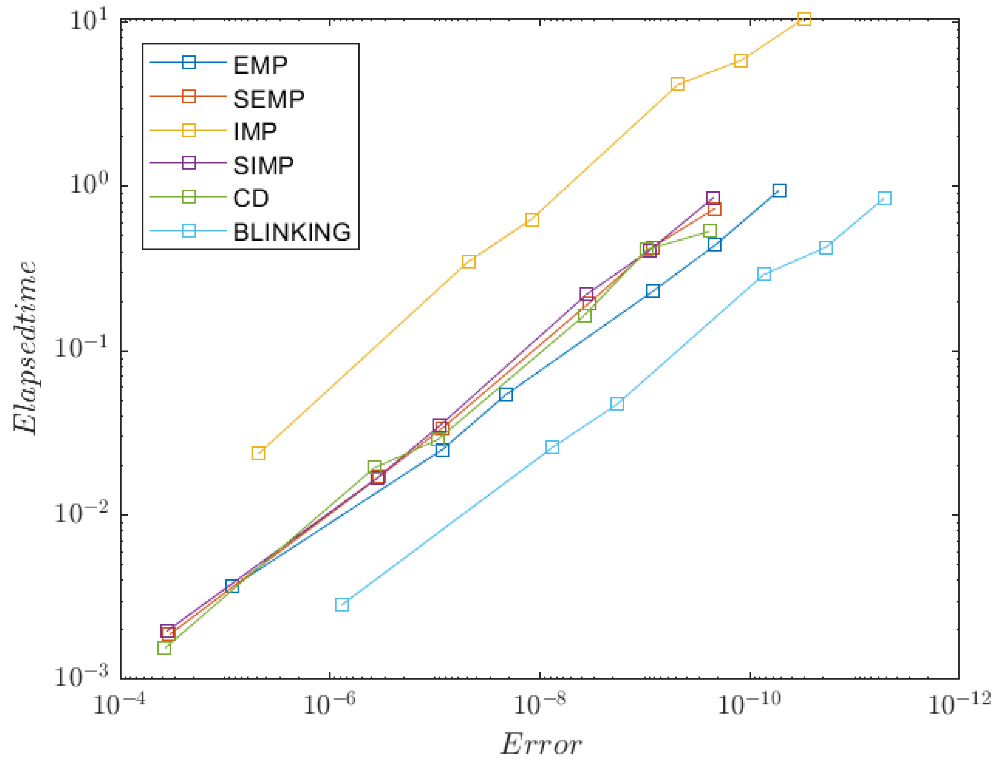
2.1. Shooting Method

Let us consider a standard approach for solving nonlinear boundary value problems described by the second-order ordinary differential equations also known as the shooting method [13]:

$$\begin{array}{c}{y}^{″}\left(x\right)=f(x,y,y^{\prime })\end{array}$$

(1)

In this paper, we consider ordinary differential equations with a nonlinear right-hand side function, and Dirichlet boundary conditions (boundary conditions of the first kind) are defined over an open interval $a<x<b$ with the following boundary conditions:

$$\begin{array}{c}y\left(a\right)=\alpha \\ y\left(b\right)=\beta \end{array}$$

(2)

To solve the designated problem, one should formulate the general Cauchy problem by replacing the Dirichlet boundary conditions with the initial conditions of the Cauchy problem. The $y\left(a\right)$ will be stated the same as in the boundary value problem, and for $y^{\prime }\left(a\right)$ we will choose a $\sigma$ value that is unknown on the current solution step:

$$\begin{array}{c}y\left(a\right)=\alpha \\ y^{\prime }\left(a\right)=\sigma \end{array}$$

(3)

The overall idea of the shooting method is that one should select the $\sigma$ value so that the solution to the Cauchy problem on the right edge is as close as possible to the right-boundary condition $y\left(b\right)$. In other words, when solving this problem, one needs to simultaneously adjust the direction of the shot using the value on the right boundary:

$$\begin{array}{c}y\left(b\right)=g\left(\sigma \right)\end{array}$$

(4)

It is possible to rewrite the problem as a nonlinear equation, which directly depends on the $\sigma$ parameter:

$$\begin{array}{c}G\left(\sigma \right)=g\left(\sigma \right)-\beta \end{array}$$

(5)

Here, one needs to minimize the G($\sigma$) value. To achieve this goal, we will apply a shooting method with a correction to the initial conditions using the Secant method [14]. Typically, such a method can be written as follows:

$$\begin{array}{c}{x}_{k+1}=x_k-{\displaystyle \frac{f\left(x_k\right)·(x_k-x_{k-1})}{f\left(x_k\right)-f\left(x_{k-1}\right)}}\hfill \end{array}$$

(6)

Among the methods with fast (quadratic) convergence, the Secant method is the optimal choice. For example, the broadly used Newton’s method has some disadvantages because the initial approximation must be set in a small neighborhood of the sought minimum, which proves to be challenging for some problems. It also can have problems with convergence, and if the function has a point near the inflection point, then the improper choice of the initial conditions may result in the looping of Newton’s method inside the area of a false extremum.

The above-mentioned shortcomings of Newton’s method can be avoided by using its modification—the Secant method. This method allows for the replacement of the second order derivative in Newton’s formula with its linear approximation. It can be shown that $x_{k+1}$ is the intersection point, with the abscissa axis of the secant line passing through points $x_k$ and $x_{k-1}$. The Secant method possesses guaranteed convergence, which is usually achieved by higher computational costs.

In our case, we can iteratively change the $\sigma$ parameter and use the acquired error at the right edge:

$$\begin{array}{c}{\sigma }_{k+1}={\sigma }_k-{\displaystyle \frac{G\left({\sigma }_k\right)·({\sigma }_k-{\sigma }_{k-1})}{G\left({\sigma }_k\right)-G\left({\sigma }_{k-1}\right)}}\hfill \end{array}$$

(7)

where

• ${\sigma }_{k+1}$—new initial conditions,
• ${\sigma }_k$—initial conditions from the previous shot,
• ${\sigma }_{k-1}$—initial conditions of the shot before the last one,
• $G\left({\sigma }_k\right)$ and $G\left({\sigma }_{k-1}\right)$—corresponding errors in an attempt to reach the boundary conditions.

In the equation for $G\left({\sigma }_k\right)$, $g\left({\sigma }_k\right)$ is the value acquired after applying a numerical integration method to the entire trajectory. Let us compare different methods that are of interest in this study using scheme (7).

To launch the shooting method, it is required to set an initial slope guess for ${\sigma }_1$. This is usually achieved by taking into account the physical properties of the original equation; ${\sigma }_2$ in this case, it is another initial guess for the Secant method, which slightly differs from the first one:

$$\begin{array}{c}{\sigma }_2={\sigma }_1+ϵ\hfill \end{array}$$

(8)

where

• $ϵ=0.01$ as an example—a small value of deviation between two initial shots.

Rewriting second-order differential Equation (1) as system of first-order ODEs yields:

$$\left\{\begin{array}{c}{y}_1^{\prime }=y_2\hfill \\ y_2^{\prime }=f(x,y_1,y_2)\hfill \end{array}\right.$$

(9)

with initial conditions $y_1\left(a\right)=\alpha$; $y_2\left(a\right)=\sigma$. Thus, the shooting error depends on the value $y_1$, and the Equation (5) can be written as $G\left(\sigma \right)=y_1\left(b\right)-\beta$. Thus, it is necessary to evaluate the error in expansion of finite-difference schemes to Taylor series.

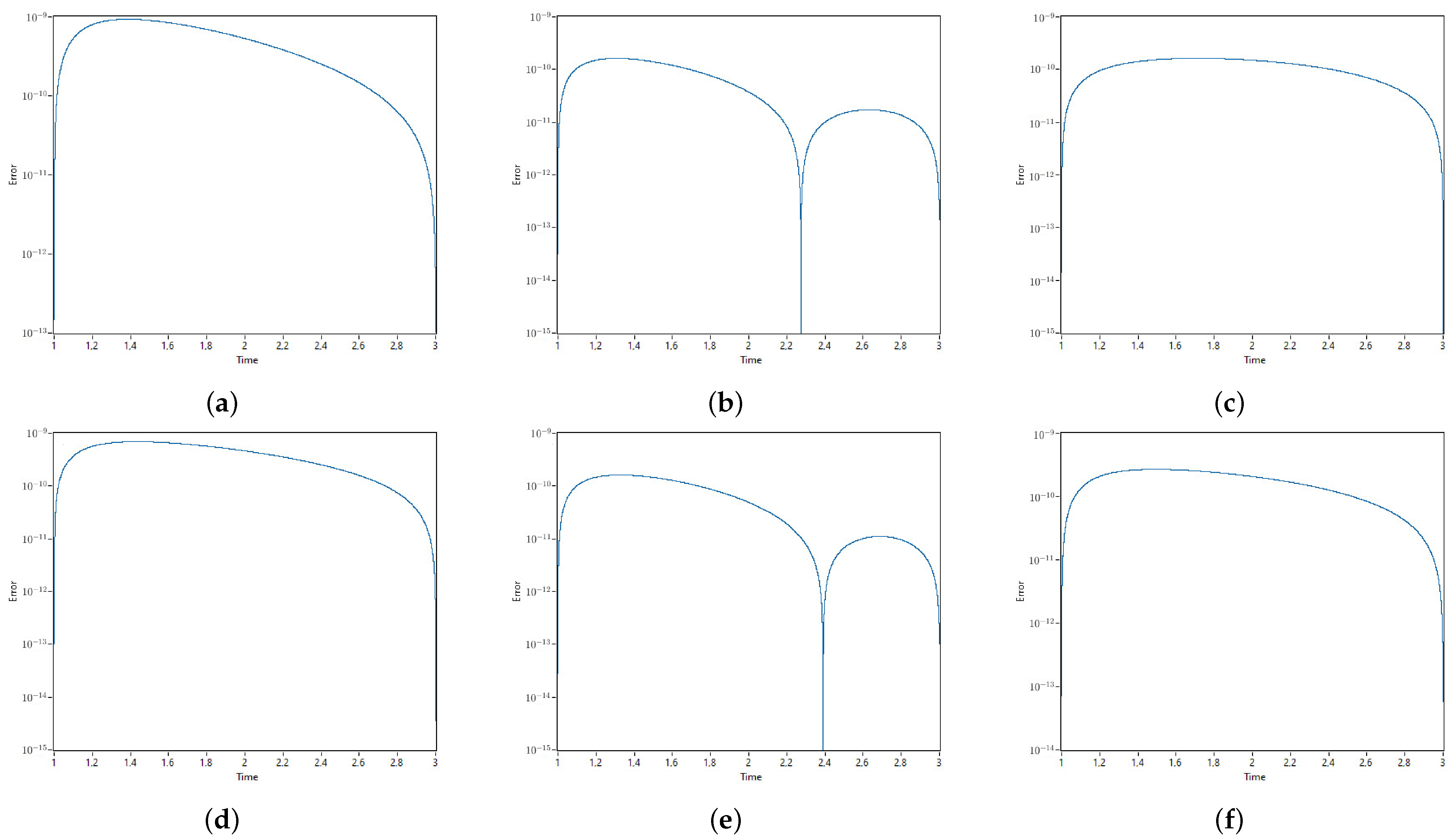
The shooting method, which reduces the solution to the boundary value problem to calculating several solutions of the Cauchy problem, works well if the solution is not highly dependent on $\sigma$. Otherwise, the system becomes computationally unstable, even if the solution to the problem is only slightly sensitive to the initial conditions.

We will use the solution acquired by the Dormand–Prince 8 method (DOPRI78) as a reference method for estimating the errors.

2.2. Semi-Explicit and Semi-Implicit Numerical Integration

Recently, some new numerical methods based on semi-explicit and semi-implicit integration principles were introduced and found to be efficient not only for solving Hamiltonian systems [12,15,16] but were also reasonably applicable to general IVPs. Semi-implicit methods can significantly outperform not only classical explicit and implicit Runge–Kutta methods but also some of the state-of-the-art algorithms, such as the Gragg–Bulirsch–Stoer extrapolation method, being superior in terms of computational efficiency and phase space structure preservation.

Definition 1.

Semi-explicit methods can only be applied to systems of order 2 and higher due to their specific principles of calculations [12]. The semi-explicit method assumes that the state variable value, which is already calculated during the current solution step, can be used to calculate the rest of the variables.

Let us consider several examples of semi-explicit and semi-implicit integration.

The semi-explicit midpoint method (SEMP) is a modification of the well-known explicit midpoint method [17]. SEMP uses the previously calculated values on the same timestep for approximating the rest of the state variables in the first part of the method’s formula:

$$\begin{array}{c}{y}_1^{n+{\displaystyle \frac{1}{2}}}=y_1^n+{\displaystyle \frac{h}{2}}·f_1(x,y_1^n,y_2^n)\hfill \\ y_2^{n+{\displaystyle \frac{1}{2}}}=y_2^n+{\displaystyle \frac{h}{2}}·f_2(x,y_1^{n+{\displaystyle \frac{1}{2}}},y_2^n)\hfill \\ y_1^{n+1}=y_1^n+h·f_1(x+{\displaystyle \frac{h}{2}},y_1^{n+{\displaystyle \frac{1}{2}}},y_2^{n+{\displaystyle \frac{1}{2}}})\hfill \\ y_2^{n+1}=y_2^n+h·f_2(x+{\displaystyle \frac{h}{2}},y_1^{n+{\displaystyle \frac{1}{2}}},y_2^{n+{\displaystyle \frac{1}{2}}})\hfill \end{array}$$

(10)

The general idea of semi-implicit methods is similar, but they require resolving the implicitness that appears when a variable implicitly depends on itself in the right-hand side function. However, contrary to fully implicit methods, semi-implicit integration possesses a one-dimensional implicitness, which assumes fewer computational costs for resolving. In many practical cases, one-dimensional implicitness can be resolved analytically, making the method similar to numerical-analytic Strang splitting. In cases when the analytical solution cannot be found (e.g., in the case of a trigonometric or exponential function of a state variable in RHS), the implicitness can be resolved by using fixed-point iterations or Newton’s method. The semi-implicit midpoint method (SIMP) for two-dimensional linear autonomous IVP can be defined as follows:

$$\begin{array}{c}{y}_1^{n+{\displaystyle \frac{1}{2}}}=y_1^n+{\displaystyle \frac{h}{2}}·f_1(x,y_1^{n+{\displaystyle \frac{1}{2}}},y_2^n)\hfill \\ y_2^{n+{\displaystyle \frac{1}{2}}}=y_2^n+{\displaystyle \frac{h}{2}}·f_2(x,y_1^{n+{\displaystyle \frac{1}{2}}},y_2^{n+{\displaystyle \frac{1}{2}}})\hfill \\ y_1^{n+1}=y_1^n+h·f_1(x+{\displaystyle \frac{h}{2}},y_1^{n+{\displaystyle \frac{1}{2}}},y_2^{n+{\displaystyle \frac{1}{2}}})\hfill \\ y_2^{n+1}=y_2^n+h·f_2(x+{\displaystyle \frac{h}{2}},y_1^{n+{\displaystyle \frac{1}{2}}},y_2^{n+{\displaystyle \frac{1}{2}}})\hfill \end{array}$$

(11)

It is worth noticing that if the system of differential equations does not contain the implicit state variable in their right-hand side function, the resolving of implicitness is meaningless and the semi-implicit methods become semi-explicit ones. Thus, the SEMP method can be considered a combination of Euler and Euler–Cromer methods taken with a half step ($E_h\circ C_{{\displaystyle \frac{h}{2}}}$), and the SIMP method can be considered as a combination of the Euler method and the D-method taken with a half step ($E_h\circ D_{{\displaystyle \frac{h}{2}}}$) [16].

To make all the considered methods exist, in our study we will consider test systems where at least one of the equations of the resulting algebraic system is implicit. In other words, we will consider differential equations of the second order, which necessarily contain a differentiable term of the first order.

The semi-explicit and semi-implicit approaches can be applied to spatially discretized partial differential equations as well. For example, in the case of the heat equation, semi-discretized by the standard central difference formula, the simplest semi-explicit method is the successive displacement version of the usual FTCS (forward-time, centered-space) method. On the other hand, the semi-implicit idea yields the UPFD (unconditionally positive finite difference) method [18].

The midpoint version of this approach for the diffusion-advection equation is elaborated on in paper [19], where the term “pseudo-implicit” is used instead of “semi-implicit”.

Let us consider the semi-implicit numerical integration of BVPs in more detail.

2.3. Semi-Implicit CD-Methods

Definition 2.

Using the composition of semi-explicit and semi-implicit Euler methods, which form a pair of so-called adjoint methods of order 1, one can obtain a symmetric integration method [12] of order 2.

It is also possible to rearrange these counterparts and choose whether to calculate the part with implicitness first or second [16]. The proposed method is called the CD numerical method of accuracy order 2, and for second-order IVP it can be written as follows:

$$\begin{array}{c}{y}_1^{n+{\displaystyle \frac{1}{2}}}=y_1^n+{\displaystyle \frac{h}{2}}·f_1(x+{\displaystyle \frac{h}{2}},y_1^n,y_2^n)\hfill \\ y_2^{n+{\displaystyle \frac{1}{2}}}=y_2^n+{\displaystyle \frac{h}{2}}·f_2(x+{\displaystyle \frac{h}{2}},y_1^{n+{\displaystyle \frac{1}{2}}},y_2^n)\hfill \\ y_2^{n+1}=y_2^{n+{\displaystyle \frac{1}{2}}}+{\displaystyle \frac{h}{2}}·f_2(x+{\displaystyle \frac{h}{2}},y_1^{n+{\displaystyle \frac{1}{2}}},y_2^{n+1})\hfill \\ y_1^{n+1}=y_1^{n+{\displaystyle \frac{1}{2}}}+{\displaystyle \frac{h}{2}}·f_1(x+{\displaystyle \frac{h}{2}},y_1^{n+1},y_2^{n+1})\hfill \end{array}$$

(12)

Let us recompose the finite-difference scheme in a way that reduces the number of arithmetical operations:

$$\begin{array}{c}{y}_2^{n+{\displaystyle \frac{1}{2}}}=y_2^n+{\displaystyle \frac{h}{2}}·f_2(x+{\displaystyle \frac{h}{2}},y_1^n,y_2^{n+{\displaystyle \frac{1}{2}}})\hfill \\ y_1^{n+1}=y_1^n+h·f_1(y_2^{n+{\displaystyle \frac{1}{2}}})\hfill \\ y_2^{n+1}=y_2^{n+{\displaystyle \frac{1}{2}}}+{\displaystyle \frac{h}{2}}·f_2(x+{\displaystyle \frac{h}{2}},y_1^{n+1},y_2^{n+{\displaystyle \frac{1}{2}}})\hfill \end{array}$$

(13)

2.4. Blinking Method Modification

It is known that semi-explicit and semi-implicit methods are efficient for solving autonomous systems of ordinary differential equations. However, the performance of these methods on systems that involve an independent variable in their equations has not been thoroughly investigated. The behavior of these integrators can be unpredictable, especially if the initial equation is stiff [20]. Let us consider a way to improve the convergence of the semi-implicit methods and prove it by analyzing the Taylor series expansions.

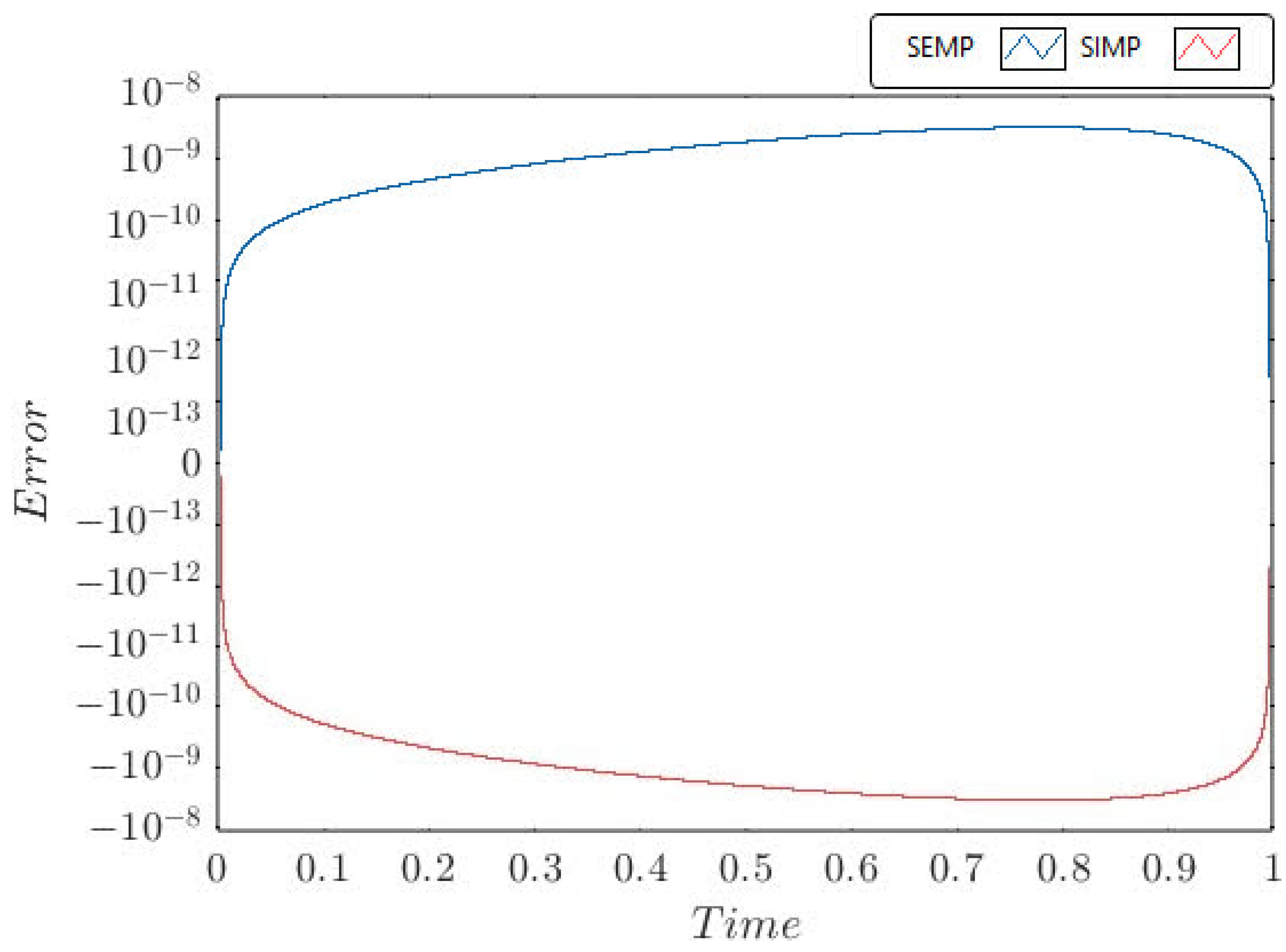
Theorem 1.

The truncation errors of semi-explicit midpoint and semi-implicit midpoint methods may have different signs.

Proof. 

Consider the Taylor series expansion over the general scheme for the numerical integration method:

$$\begin{array}{c}\begin{array}{cc}\hfill y_1^{n+1}& =y_1^n+h·{\dot{y}}_1^n+{\displaystyle \frac{h^2}{2}}·{\ddot{y}}_1^n+{\displaystyle \frac{h^3}{6}}·{\stackrel{⃛}{y}}_1^n=\hfill \\ \hfill & =y_1^n+h·y_2^n+{\displaystyle \frac{h^2}{2}}·f(x_n,y_1^n,y_2^n)+{\displaystyle \frac{h^3}{6}}·({\displaystyle \frac{\partial f(x_n,y_1^n,y_2^n)}{\partial y_1}}+{\displaystyle \frac{\partial f(x_n,y_1^n,y_2^n)}{\partial y_2}})\hfill \end{array}\hfill \end{array}$$

(14)

The Taylor series expansion for the Euler–Cromer (C) method is as follows:

$$\begin{array}{c}{y}_1^{n+1}=y_1^n+h·y_2^n=y_1^n+h·y_2^n+{\displaystyle \frac{h^2}{2}}·f(x_n,y_1^{n+{\displaystyle \frac{1}{2}}},y_2^n)\hfill \end{array}$$

(15)

when

$$\begin{array}{c}f(x_n,y_1^{n+{\displaystyle \frac{1}{2}}},y_2^n)=f(x_n,y_1^n,y_2^n)+{\displaystyle \frac{h}{2}}·{\displaystyle \frac{\partial f(x_n,y_1^n,y_2^n)}{\partial y_1}}\hfill \end{array}$$

Subtracting (15) from (14), one can obtain the following error equation:

$$\begin{array}{c}er{r}_C=-{\displaystyle \frac{h^3}{12}}·{\displaystyle \frac{\partial f(x_n,y_1^n,y_2^n)}{\partial y_1}}+{\displaystyle \frac{h^3}{6}}·{\displaystyle \frac{\partial f(x_n,y_1^n,y_2^n)}{\partial y_2}}\hfill \end{array}$$

(16)

Consider the Taylor series expansion for the D-method:

$$\begin{array}{c}{y}_1^{n+1}=y_1^n+h·y_2^{n+{\displaystyle \frac{1}{2}}}=y_1^n+h·y_2^n+{\displaystyle \frac{h^2}{2}}·f(x_n,y_1^{n+{\displaystyle \frac{1}{2}}},y_2^{n+{\displaystyle \frac{1}{2}}}),\hfill \end{array}$$

(17)

where

$$\begin{array}{c}f(x_n,y_1^{n+{\displaystyle \frac{1}{2}}},y_2^{n+{\displaystyle \frac{1}{2}}})=f(x_n,y_1^n,y_2^n)+{\displaystyle \frac{h}{2}}·{\displaystyle \frac{\partial f(x_n,y_1^n,y_2^n)}{\partial y_1}}+{\displaystyle \frac{h}{2}}·{\displaystyle \frac{\partial f(x_n,y_1^n,y_2^n)}{\partial y_2}}\hfill \end{array}$$

Subtracting (17) from (14), one can obtain the following error equation:

$$\begin{array}{c}er{r}_D=-{\displaystyle \frac{h^3}{12}}·{\displaystyle \frac{\partial f(x_n,y_1^n,y_2^n)}{\partial y_1}}-{\displaystyle \frac{h^3}{12}}·{\displaystyle \frac{\partial f(x_n,y_1^n,y_2^n)}{\partial y_2}}\hfill \end{array}$$

(18)

Thus, the SEMP and SIMP methods differ only in the first part (the Euler–Cromer and D methods, respectively) of the scheme, whereas the second part (the Euler method) remains the same. Thus, both first terms in (16) and (18) are equal. However, the second terms differ and possess different signs. Based on the fact that the Euler–Cromer method and D-method are adjoints, one can conclude that SEMP and SIMP errors will have different signs, provided that there is a significant impact from the second term.    □

The key idea of the current research is to utilize the fact that semi-explicit and semi-implicit midpoint methods can provide opposite numerical errors to reduce the overall error of the BVP solution. For example, one can apply the semi-explicit method (10) for all of the odd steps and the semi-implicit method (11) for the remaining even steps, thus maintaining the order of the resulting numerical integration scheme while simultaneously reducing its truncation error.

In Figure 1, ${\Phi }_1$—SEMP method; ${\Phi }_2$—SIMP method; h—stepsize; $y^i=\left(\begin{array}{c}{y}_1^i\\ y_2^i\end{array}\right)$; $x^i=x+i·h$.

One may notice that there are other versions of this hybrid method possible, for example, the scheme that assumes the averaging of the solutions obtained by semi-implicit and semi-explicit counterparts, or the direct composition scheme. However, despite both these variants being applicable, they are less numerically efficient than the blinking solver, and the parallel composition (i.e., averaging) will result in a non-symmetric scheme. Therefore, we believe that switching the right-hand side function is the most efficient approach to solving the convergence issue. Let us investigate the properties of the developed method further.

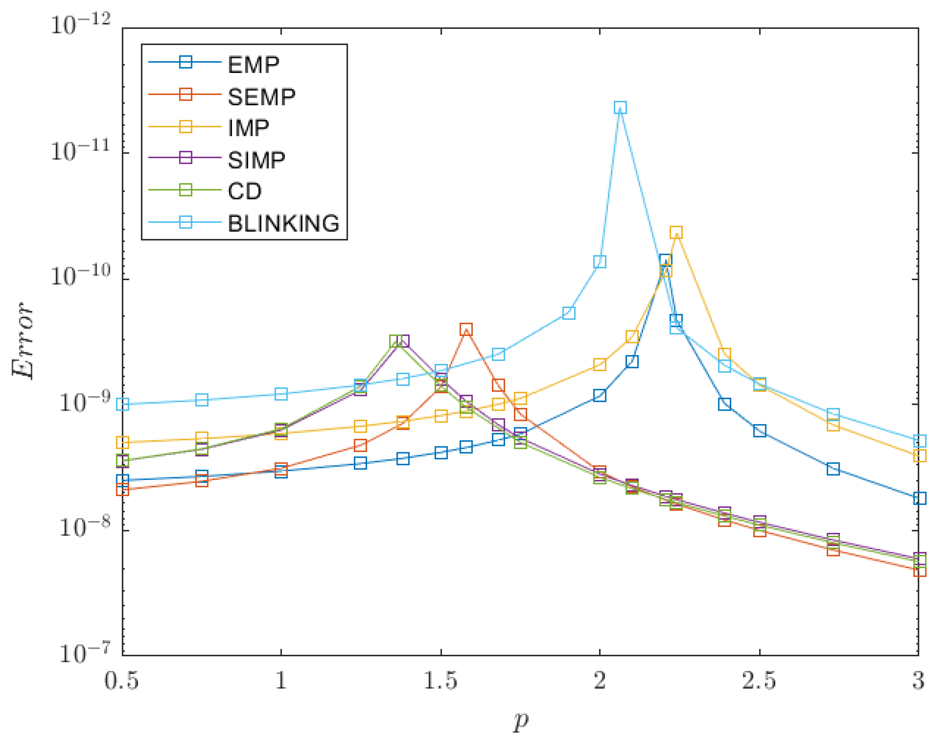
2.5. The Stability Analysis of the Semi-Explicit and Semi-Implicit Methods

Numerical stability is one of the crucial properties of numerical methods. The stability analysis of the proposed numerical scheme is possible while investigating a Dahlquist test problem of dimension 2 or higher due to the specific type of calculations of semi-implicit methods. Thus, one can analyze the methods’ numerical stability by applying the same technique as was previously shown in [11]. Let us consider a two-dimensional test problem:

$$\dot{x}=\left(\begin{array}{cc}{\alpha }_{11}& {\alpha }_{12}\\ {\alpha }_{21}& {\alpha }_{22}\end{array}\right)x$$

(19)

where the matrix

$$A=\left(\begin{array}{cc}{\alpha }_{11}& {\alpha }_{12}\\ {\alpha }_{21}& {\alpha }_{22}\end{array}\right)$$

(20)

has complex conjugate eigenvalues. Let us construct matrix A with eigenvalues

$${\lambda }_{1,2}=\sigma \pm j\omega$$

(21)

in normal Jordan form:

$$A=\left(\begin{array}{cc}\sigma & \omega \\ -\omega & \sigma \end{array}\right)$$

(22)

One can find the stability region the same way as in the case of a one-dimensional Dahlquist test problem:

$$\dot{x}=\lambda x$$

(23)

by expressing

$$x^{n+1}=R\left(h\lambda \right)x^n$$

(24)

and finding an area on a complex plane, where the maximum modulo eigenvalue of matrix $R\left(h\lambda \right)$ lies within a unit circle:

$$max\left|eig\right(R\left(h\lambda \right)\left)\right|<1$$

(25)

The real systems can possess an asymmetric matrix A, and to handle this issue we introduce the following parameters:

$$r={\displaystyle \frac{{\alpha }_{12}}{{\alpha }_{21}}},k={\displaystyle \frac{{\alpha }_{11}}{{\alpha }_{22}}}$$

(26)

Definition 3.

At $k=0$, the matrix is the most asymmetric; specifically, it can be a matrix in the Frobenius normal form. At $k=1$, the matrix A is the most symmetric, namely, the Jordan canonical form.

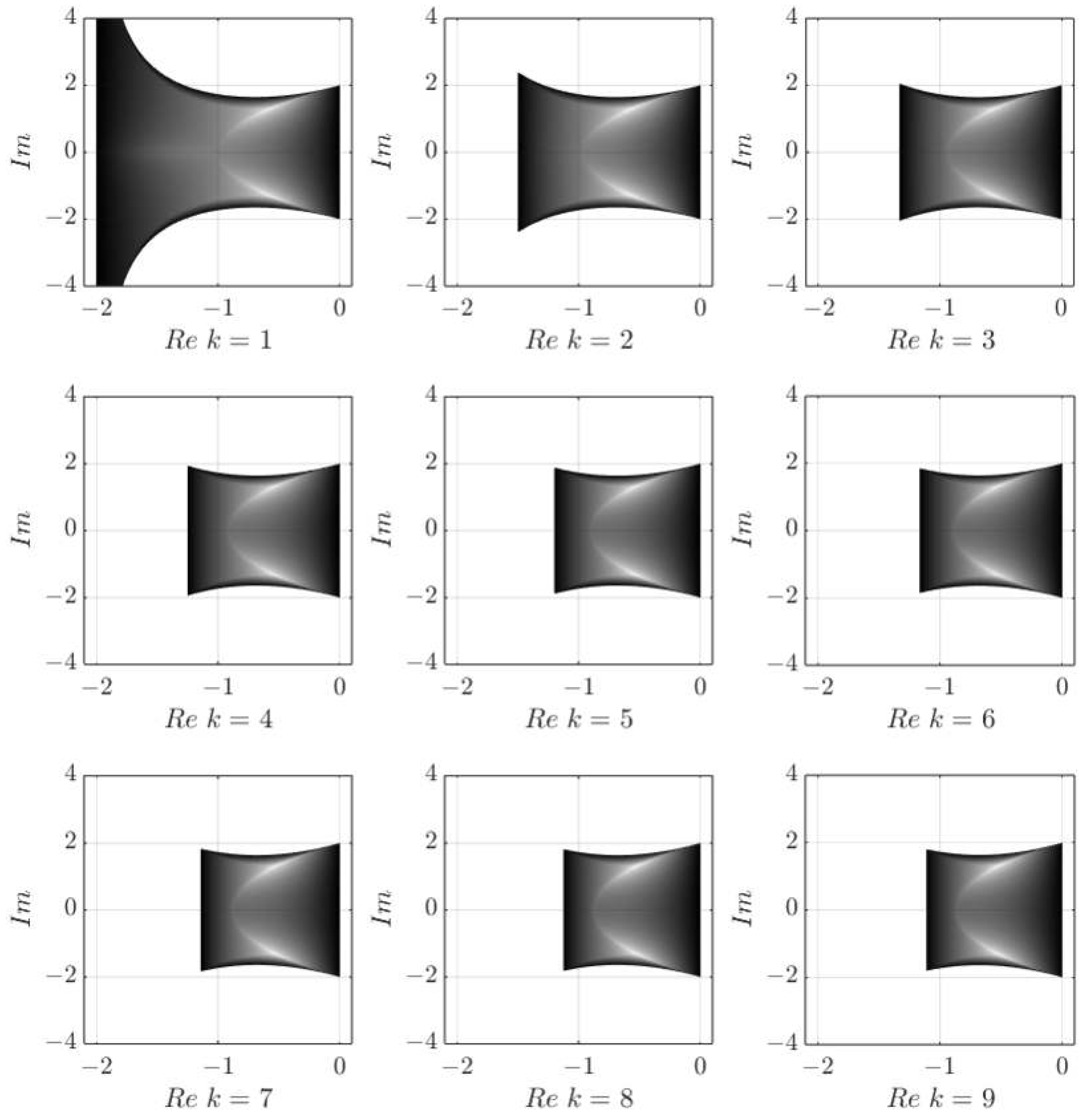
By varying the proposed parameters, one can find stability regions of the CD method with dependence on the matrix A symmetry, see Figure 2:

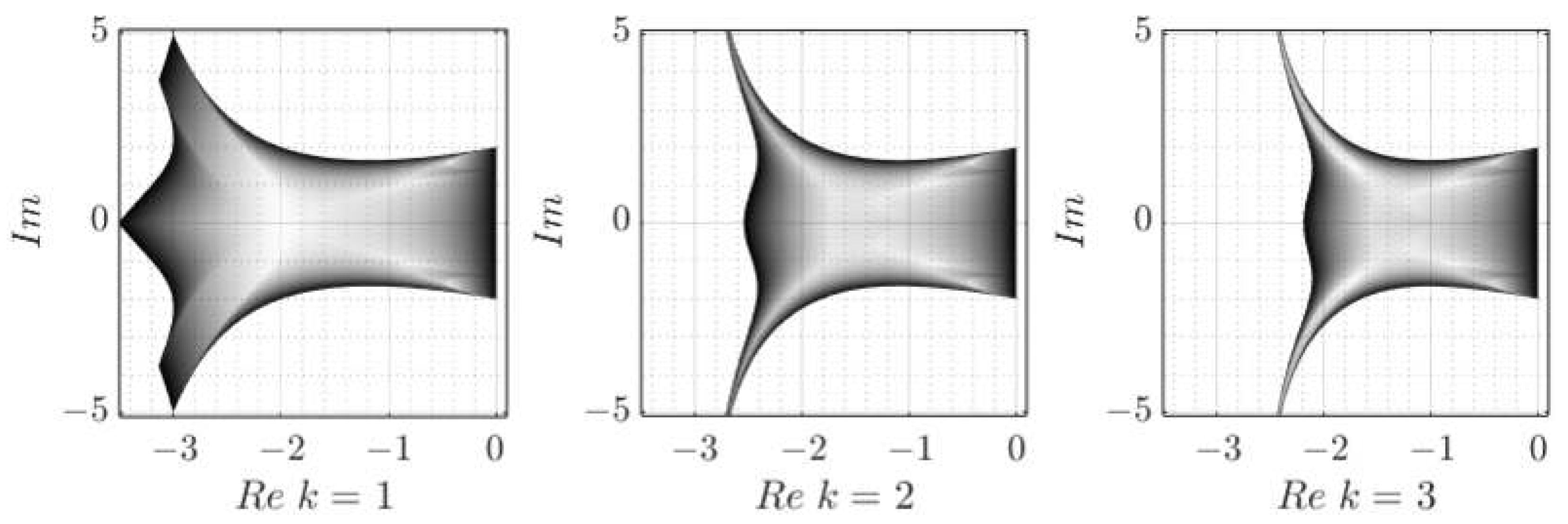
The stability regions of the SIMP method are the same as for the CD method. This is because both of these methods have the identical expansion of the first principal terms in a Taylor series for a chosen test problem. Unlike semi-implicit methods, the SEMP integration technique has quite an unusual shape of its stability region, see Figure 3:

Finally, for a newly developed “blinking” scheme the stability regions are as follows (Figure 4).

Stability analysis shows that the “blinking” method possesses larger and fewer symmetry-dependent stability regions than its semi-implicit or semi-explicit counterparts.

3. Experimental Results: Performance Test

In this section, we analyze the performance of different versions of the midpoint integration method as well as corresponding semi-implicit schemes. To evaluate and compare the investigated methods, the global maximum of the truncation error is plotted relative to the elapsed CPU time in the form of a so-called efficiency plot. The entire investigation was carried out with the Dormand–Prince 8 (DOPRI8) method as a starting solver and a reference solution. All the experiments were performed in an NI LabVIEW 2022 software environment with double floating-point precision data type.

In order to evaluate the numerical efficiency of the proposed numerical schemes, let us consider a set of linear and non-linear test BVPs.

3.1. Test System I

Let the differential equation $y^{″}+{\displaystyle \frac{2}{x}}{y}^{\prime }+{\displaystyle \frac{1}{x^4}}y=0$ be set in the interval $[{\displaystyle \frac{1}{3\pi }};1]$ with boundary conditions $y\left({\displaystyle \frac{1}{3\pi }}\right)=0$ and $y\left(1\right)=sin1$ [21].

The second-order equation can be converted into the following system of first-order ODEs:

$$\left\{\begin{array}{c}{y}_1^{\prime }=y_2\hfill \\ y_2^{\prime }=-{\displaystyle \frac{2}{x}}{y}_2-{\displaystyle \frac{1}{x^4}}{y}_1\hfill \end{array}\right.$$

By applying the investigated numerical methods and comparing their solutions with the reference DOPRI8 method, one can obtain a comparison graph showing the relative numerical efficiency of the considered solvers, see Figure 5.

Table 1. The integration steps used for plotting the performance plots in Figure 5.

	Point 1	Point 2	Point 3	Point 4	Point 5	Point 6
Stepsize	${10}^{-3}$	${10}^{-4}$	${10}^{-5}$	$5·{10}^{-6}$	$2.5·{10}^{-6}$	${10}^{-6}$

contains the stepsizes we used in our experiments.

The discrete models written in C-style code for this test system obtained using all of the integration methods discussed in this paper are presented in Appendix A.

One can see from Figure 5 that all semi-explicit and semi-implicit methods show the best performance while solving Problem 1. The implicit midpoint (IMP) method provides greater precision but requires significantly more calculation time due to the required implicitness resolution involving multiple calls of the right-hand side function. The explicit midpoint method possesses slightly lower accuracy compared to other methods. Semi-explicit (SEMP) and semi-implicit (CD, SIMP) methods demonstrate similar performance because their asymptotical expansions are close for this simple system. It is important to note that in this experiment, all methods used the same number of shots during the shooting method iterations.

3.2. Test System 2

Let us consider another example of BVP [22], which can be represented by the following differential equation $y^{″}+{\displaystyle \frac{1}{8}}y{y}^{\prime }=(4+{\displaystyle \frac{1}{4}}{x}^3)$ on a given open interval $1<x<3$ with Dirichlet boundary conditions $y\left(1\right)=17$ and $y\left(3\right)={\displaystyle \frac{43}{3}}$. Although there is an exact solution where $y\left(x\right)=x^2+{\displaystyle \frac{16}{x}}$, we still use DOPRI8 as a reference method to double-check the error.

The system’s equation can be written as IVP:

$$\left\{\begin{array}{c}{y}_1^{\prime }=y_2\hfill \\ y_2^{\prime }=-{\displaystyle \frac{1}{8}}{y}_2{y}_1+4+{\displaystyle \frac{1}{4}}{x}^3\hfill \end{array}\right.$$

The solution time steps are given in Table 2. Let us investigate the considered numerical schemes to find approximate solutions and evaluate their truncation errors.

One can see from Figure 6 and Figure 7 that the semi-implicit midpoint method and CD are slightly more accurate while solving Test Problem 2 than other considered schemes, which confirms the applicability of these approaches to solving nonlinear equations. The results obtained by using the EMP and SEMP methods are very similar to each other. The implicit midpoint method provides greater accuracy but simultaneously requires a longer calculation time to find the solution. The acquired results can be explained by the influence of nonlinearity. All of the proposed methods were analyzed with the same number of shots during the shooting method iteration.

Table 2. The integration steps used for plotting the performance plots in Figure 7.

	Point 1	Point 2	Point 3	Point 4	Point 5
Stepsize	${10}^{-2}$	${10}^{-3}$	${10}^{-4}$	$2.5·{10}^{-5}$	${10}^{-5}$

Table 2. The integration steps used for plotting the performance plots in Figure 7.

	Point 1	Point 2	Point 3	Point 4	Point 5
Stepsize	${10}^{-2}$	${10}^{-3}$	${10}^{-4}$	$2.5·{10}^{-5}$	${10}^{-5}$

It is important to note the similar behavior of truncation errors in both implicit and semi-implicit schemes. The sharp decrease in error value nearly to zero when using these methods is probably due to the presence of points where the discretization closely approximates the true solution.

3.3. Test System 3

As a third system, we considered the differential equation $y^{″}-7y^{\prime }+12y=4e^{2x}$, which is set in the interval $[0;1]$ with boundary conditions $y\left(0\right)=3$ and $y\left(1\right)=5e^2$ [23].

This equation can be rewritten as the following ODE system:

$$\left\{\begin{array}{c}{y}_1^{\prime }=y_2\hfill \\ y_2^{\prime }=7y_2-12y_1+4e^{2x}\hfill \end{array}\right.$$

Thus, it can be solved using numerical integration schemes under investigation. However, the previously mentioned problem of convergence comes to the spot because test system 3 demonstrates solutions of an exponential nature. The initial experiments revealed a bad convergence of semi-implicit methods, and thus we investigated this problem in more detail.

3.3.1. Resolving the Problem of Convergence of Semi-Implicit and Semi-Explicit Methods

During the computational experiments, it was discovered that the investigated SEMP and SIMP methods possess a truncation error of similar value but of opposite signs, see Figure 8. This fact allowed us to suggest whether these errors can compensate for each other if the SEMP and SIMP methods are composed into a single solution scheme. For this purpose, the semi-explicit midpoint and semi-implicit midpoint methods were used in an alternating manner, where semi-explicit computation was applied at odd steps of the solution, and semi-implicit computation was applied at even steps. Let us call this approach the Blinking integration method. One can see from Figure 9 that the performance of semi-implicit methods [20] can be significantly improved by applying a composition of semi-implicit and semi-explicit right-hand side function calculation.

3.3.2. Experimental Results

By analyzing the results shown in Figure 9, one can conclude that the results of the SEMP, SIMP, and CD methods are very close to each other while solving Test Problem 3. These methods appear to be significantly less effective on this exponential problem than the classical explicit EMP method, which proved to be suitable for non-stiff problems with solutions of an exponential nature. This means that when solving such systems, we cannot take full advantage of semi-implicit and semi-explicit integration. The implicit midpoint method provides significantly more accurate results than its counterparts but still requires much more computational resources and, consequently, estimates more calculation time.

It is worth noting that methods have different number of shots during the shooting method iterations. The corresponding numbers of shots and stepsizes are given in

Table 3. The number of the shooting method iterations for the proposed numerical schemes.

		Point 1	Point 2	Point 3	Point 4	Point 5	Point 6
	Stepsize	${10}^{-3}$	${10}^{-4}$	$5·{10}^{-5}$	${10}^{-5}$	$5·{10}^{-6}$	$2.5·{10}^{-6}$
Method
EMP		8	5	6	5	5	6
SEMP		3	3	3	4	5	4
IMP		2	5	4	6	4	3
SIMP		3	3	3	5	5	5
CD		2	4	3	4	5	3
BLINKING		5	5	5	6	4	4

.

The Blinking method, on the other hand, is perfectly designed to improve the efficiency of solving exponential systems when conventional semi-implicit methods can experience convergence loss. In this scheme, the order of accuracy of the original SEMP and SIMP methods is preserved while their general efficiency vastly increases. Applying the blinking method does not require significant overheads in computational costs.

To verify the impact of initial conditions on the efficiency of the proposed scheme, several additional experiments were performed. The initial boundary condition $\alpha$ has been modified so that the trajectory of the solution remains unchanged. Truncation error estimation under other initial conditions is represented in the Appendix B.

3.4. Parametric Analysis

To investigate the dependence between the precision of the BVP numerical solution and initial conditions, we decided to reformulate the conditions for the third equation. A special parameter P was introduced to investigate the dynamics of truncation error of investigated integration methods. Thus, the differential equation took the form of $y^{″}-7y^{\prime }+12y=4e^{Px}$.

The interval was chosen as was previously mentioned $[0;1]$; the first boundary condition was stated at $y\left(0\right)=3$, but the second boundary condition was changed to $y\left(1\right)=5e^P$. These changes have been made to ensure that the partial solution to the differential equation becomes less dependent on the constant. The discretization step was set as h = ${10}^{-5}$.

One can see from Figure 10 that the value of the independent variable has a significant impact on the general accuracy of the acquired solutions. It can be noticed that the errors of the EMP and IMP methods behave similarly, and the same similarity can be observed for SEMP and SIMP schemes while the (P) parameter is being varied. A slightly more accurate solution can be obtained by the semi-implicit and semi-explicit methods for a smaller value of the parameter in comparison with standard midpoint methods. By using the proposed Blinking method, we added the possibility of preserving the accuracy order of the solution while simultaneously increasing the general numerical efficiency of the solver. These results can be explained by the improved stability and convergence of semi-implicit numerical integration methods [11].

Not all of the aspects of how the semi-implicit methods impact the discrete simulations of the non-autonomous equations and systems of ordinary differential equations have been sufficiently investigated yet. Thus, one can use the proposed blinking scheme with care, especially when solving highly nonlinear and chaotic dynamical systems. However, the blinking scheme in no case can perform worse than its components do separately.

4. Conclusions and Discussion

In this study, we investigated and analyzed the performance of various numerical integration schemes for solving boundary problems, namely, implicit, explicit, semi-explicit, and semi-implicit midpoint methods. Several representative examples were chosen to evaluate the properties of the semi-implicit methods in comparison with their well-known fully explicit and implicit counterparts. It is shown that semi-implicit methods meet some difficulties while solving the systems with exponential solutions. We proposed a new technique of the “blinking” solver to resolve this issue by simple modifications to the existing schemes. The proposed blinking semi-implicit/semi-explicit solver can significantly increase the algebraic precision and convergence of the solution for boundary problems without additional computational overheads. It should be noted that the semi-implicit midpoint method and its CD modification are both symmetric integrators and thus are suitable for being used as basic methods in extrapolation and composition solvers of higher-accuracy orders.

Our future research will be devoted to the implementation of a blinking integration scheme with an adaptive integration stepsize and the construction of higher-order extrapolation and composition integration schemes with blinking semi-implicit/semi-explicit methods as a basic integrator.